A methodology for temperature option pricing in the equatorial regions

Abstract

Weather derivatives are financial instruments that can be used by organizations or individuals to hedge risks associated with adverse weather conditions. Weather conditions can directly decrease profits by affecting the volume of sales or costs. This paper develops a methodology for temperature option pricing in equatorial regions. In this approach, temperature is forecast by combining deterministic and stochastic models. We find that forecasting daily temperature with a model that combines a truncated third-order Fourier series with a mean reversion stochastic process proves the most accurate for pricing the options. The methodology is calibrated with data gathered in Bogotá, Colombia, using Monte Carlo simulations.

1. Introduction

For over two decades, American, Asian, and European financial derivatives markets have traded weather derivatives, which hedge organizations and individuals against risks arising from different adverse weather conditions (Weber, 2009). Weather derivatives are used as part of risk management strategies to hedge the risk from non-catastrophic weather events (Alexandridis & Zapranis, 2012). The energy consumption, energy generation, agriculture, retail, travel, transportation, entertainment, government, and construction industries are the main economic sectors that use weather derivatives (Alexandridis & Zapranis, 2012; Chantarat et al., 2011; Elias et al., 2017; Islip et al., 2021; Jewson & Brix, 2005; Turvey, 2001).

The traditional choice for hedging risks has been the insurance market. However, in contrast to insurance contracts, weather derivatives are designed to (i) hedge against non-catastrophic weather events and (ii) avoid the usual hurdles of moral hazard issues (Alexandridis & Zapranis, 2012; Rappenglück et al., 2004).

In general, weather derivatives can be found in the form of futures, forward or option contracts, which depend on the values of underlying weather variables such as the temperature, rainfall, wind, solar irradiance, snowfall, and humidity (Cao & Wei, 2000). According to the Weather Risk Management Association (WRMA), approximately 75% of weather derivatives transactions are based on temperature (Barrieu & Scaillet, 2009). The Chicago Mercantile Exchange (CME) offers various temperature futures and options contracts in 46 cities around the world: 24 in the USA, 10 in Europe, 6 in Canada, 3 in Australia, and 3 in Japan (CME, 2005). However, the weather derivatives market is incipient or missing in many countries in the equatorial region.

Temperature derivatives can provide a reliable hedge for various economic sectors against the risks posed by unanticipated changes in temperature (Campbell & Diebold, 2005; Islip et al., 2021). These securities can prove useful to participants in agricultural markets because crops and fields are vulnerable to temperature fluctuations (Brown & Kshirsagar, 2015). The fundamental fact underlying this example is that temperature derivatives act as hedges against a “volume” risk (see, for instance, the discussion in Brockett et al. (2005)). When exercised, the temperature derivative payoff is independent of whether any actual loss occurs in harvest (Alexandridis & Zapranis, 2012). This principle also applies to the case of energy consumption, where the temperature weather derivatives play a significant hedging role (Dutton, 2002; Elias et al., 2017).

The problem of designing derivatives on non-tradable underlying variables such as temperature has been the subject of much theoretical research in the last two decades (see, for instance, Alaton et al. (2002) and Benth and Šaltytė-Benth (2005)). These approaches seek to extend methods based on stochastic processes that are applied in the theory of financial derivatives. There is also an empirical approach, as exemplified in the work by Swishchuk and Cui (2013). The present work falls within this line of research, although our methods are closer in spirit to those in Campbell and Diebold (2005).

This study presents a methodology for option pricing in equatorial regions, specifically in the case of temperature as the underlying index, which is applied to a case study: Bogotá, Colombia. Section 2 describes the temperature modeling approach and the option pricing model. Section 3 applies the methodologies of Section 2 to the case study. Finally, Section 4 presents the conclusions.

2. Methodology

Our methodology consists of a model that more accurately describes the daily average temperature (DAT) to price temperature options. In principle, DAT modeling may lead to more accurate pricing than modeling of temperature indices, such as heating degree days (HDDs) or cooling degree days (CDDs) (Jewson & Brix, 2005).

The approach starts with temperature data collection, processing, and analysis, followed by specification and estimation of forecasting models. The pricing approach is framed in the context of weather derivatives and temperature options, as depicted in Figure 1.

Figure 1. General methodology for temperature option pricing.

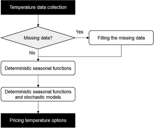
2.1. Temperature data collection

The DAT is defined as the average of the daily maximum and minimum temperatures and measured in degrees Fahrenheit (${}^{°}F$): (1) $$T_t=\frac{T_t^{\mathit{Max}}+T_t^{\mathit{Min}}}{2}$$(1) where T_t is the DAT, $T_t^{\mathit{Max}}$ is the maximum temperature, and $T_t^{\mathit{Min}}$ is the minimum temperature reported during day t. We suggest a minimum of 50 years of recent historical temperature data, which should include the effects of climate change. The data record must provide sufficient information about the maximum and minimum temperatures for every day of the year.

2.2. Filling in the missing data

The presence of missing data over some periods requires cross-referenced interpolation or more complex methods with different sources for the same information. A short list of the most common methods includes using nearby weather stations, data augmentation algorithms, state space models and a Kalman filter, neural networks (NNs), and principal component analysis (PCA) (Dunis & Karalis, 2003). In our case, missing values ($T_{t,\mathit{missing}}$) can be readily completed according to the following procedure proposed by Alexandridis and Zapranis (2012): (2) $$T_t^{\mathit{missing}}=\frac{T_t^{\mathit{avgYear}}+T_t^{\mathit{avgDay}}}{2}$$(2) (3) $$T_t^{\mathit{avgYear}}=\frac{1}{N}\sum _{\mathit{year}=1}^N{T}_t^{\mathit{year}}$$(3) (4) $$T_t^{\mathit{avgDay}}=\frac{\sum _{i=1}^7{T}_{t-i}+\sum _{i=1}^7{T}_{t+i}}{14}$$(4) where $T_t^{\mathit{avgYear}}$ is the average temperature of that particular day across N years and $T_t^{\mathit{avgDay}}$ is the average temperature of the previous plus 7 following days about the missing value.

2.3. Deterministic seasonality functions

Many different models have been proposed to describe the dynamics of DAT (Alexandridis & Zapranis, 2012). We describe the behavior of the temperature in terms of two types of components, as shown in Equation (5)(5) $$T_t=f(t)+X_t$$(5) (Lucia & Schwartz, 2002). (5) $$T_t=f(t)+X_t$$(5) where f(t) is a deterministic seasonality function of time and X_t is a stochastic process. Now, we proceed to selecting one of several possible choices for the deterministic component f(t), all of which have the same general form: a general trend that grows linearly in time and a component that seeks to capture the seasonality effects. The monthly seasonality can be captured by either dummies or a periodic function. The final selection should be based on the model accuracy: (i) root mean square error (RMSE), (ii) Akaike information criterion (AIC), and (iii) Bayesian information criterion (BIC) (Akaike, 1974; Schwarz, 1978).

• Model 1: Monthly and yearly effects are important in describing the temperature behavior, as shown in Figures 2 and 3, respectively. The simplest deterministic seasonality function allows for monthly and yearly effects using two types of variables: a numeric one for the year (Y_t) and dummy variables to model the month (M_it). Dummy variables are intuitive and enable a straightforward estimation of the effect of each month. For this model, the deterministic function is given by: (6) $$f(t)=\alpha +\omega Y_t+\sum _{i=2}^{12}{\beta }_i{M}_{i,t}$$(6)

where Y_t is the year of date t, $M_{i,t}$ is 1 if date t belongs to the i-th month or 0 otherwise, and α, ω and β_i are all constant parameters. Coefficient ω captures the annual changes in temperature associated with global warming.

Figure 2. Monthly mean temperature at Bogotá, Colombia (1961–2018). Data source: American National Oceanic and Atmospheric Administration (NOAA, 2018).

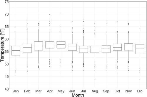
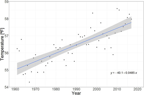
Figure 3. Yearly mean temperature at Bogotá, Colombia (1961–2018). Data source: American National Oceanic and Atmospheric Administration (NOAA, 2018).

• Model 2: Alternatively, instead of monthly dummy variables, a truncated first-order Fourier series is used as the deterministic seasonality function: (7) $$f(t)=\alpha +\omega Y_t+{\gamma }_1\hspace{0.17em}\text{sin}\hspace{0.17em}\left(\frac{2\pi t}{365}\right)+{\delta }_1\hspace{0.17em}\text{cos}\hspace{0.17em}\left(\frac{2\pi t}{365}\right)$$(7)

where γ₁ and δ₁ are constant parameters. $\text{sin}\hspace{0.17em}$ and $\text{cos}\hspace{0.17em}$ reflect the annual seasonal pattern in the evolution of the temperature.

• Model 3: We propose a second-order Fourier series to represent the deterministic seasonality function. The deterministic function of the temperature is a sum of two sine and cosine functions: (8) $$f(t)=\alpha +\omega Y_t+\sum _{i=1}^2\left[{\gamma }_i\hspace{0.17em}\text{sin}\hspace{0.17em}\left(\frac{2\pi it}{365}\right)+{\delta }_i\hspace{0.17em}\text{cos}\hspace{0.17em}\left(\frac{2\pi it}{365}\right)\right]$$(8)

γ_i and δ_i are constant parameters.

• Model 4: We propose a third-order Fourier series to represent the deterministic seasonality function: (9) $$f(t)=\alpha +\omega Y_t+\sum _{i=1}^3\left[{\gamma }_i\hspace{0.17em}\text{sin}\hspace{0.17em}\left(\frac{2\pi it}{365}\right)+{\delta }_i\hspace{0.17em}\text{cos}\hspace{0.17em}\left(\frac{2\pi it}{365}\right)\right]$$(9)

• Model 5: We propose a fourth-order Fourier series to represent the deterministic seasonality function: (10) $$f(t)=\alpha +\omega Y_t+\sum _{i=1}^4\left[{\gamma }_i\hspace{0.17em}\text{sin}\hspace{0.17em}\left(\frac{2\pi it}{365}\right)+{\delta }_i\hspace{0.17em}\text{cos}\hspace{0.17em}\left(\frac{2\pi it}{365}\right)\right]$$(10)

2.4. Deterministic seasonality functions and stochastic processes

The actual DAT is also conditioned by the recent temperature behavior. In addition to the deterministic component, DAT models should include a specific stochastic component, which we will assume follows mean-reversion dynamics (Dornier & Queruel, 2000). In addition, the DAT can present unexpected jumps from its expected value; therefore, we add a jump process to the stochastic part of the temperature model.

In summary, we assume that X_t follows a stationary mean-reverting process (Ornstein-Uhlenbeck process) (Dixit et al., 1994), which leads to the usual procedure of modeling the stochastic component of temperature (Dornier & Queruel, 2000). To estimate the temperature models using daily discrete observations, we must fully express them in discrete form. Then, we use a simple discretization of the mean-reverting process with the long-run mean zero: (11) $$X_t=\varphi X_{t-1}+{\epsilon }_t$$(11) where $\varphi$ is equal to 1 minus the speed of reversion and ${\epsilon }_t$ are i.i.d. normal random variables with mean zero and constant variance ${\sigma }_{\epsilon }^2.$

Additionally, we add a Poisson process to model the abrupt temperature events, where there is at most one jump per day (Dixit et al., 1994; Seifert & Uhrig-Homburg, 2007): (12) $$X_t=\{\begin{array}{cc}\varphi X_{t-1}+{\epsilon }_t& \text{with}\mathrm{ }\text{probability}\mathrm{ }1-\lambda \\ \varphi X_{t-1}+{\mu }_J+{\epsilon }_t& \text{with}\mathrm{ }\text{probability}\mathrm{ }\lambda \end{array}$$(12) where λ is the mean arrival rate of an event per day and μ_J is a normal random variable with mean zero and constant variance ${\sigma }_J^2.$

In summary, we have five candidate deterministic functions (f(t)) combined with two stochastic processes (X_t). We simultaneously estimate their parameters by nonlinear least squares methods:

• Mean reversion: (13) $$T_t=\varphi T_{t-1}+f(t)-\varphi f(t-1)+{\epsilon }_t$$(13)

• Mean reversion and jump process: (14) $$T_t=\{\begin{array}{cc}\varphi T_{t-1}+f(t)-\varphi f(t-1)+{\epsilon }_t& \text{with}\mathrm{ }\text{probability}\mathrm{ }1-\lambda \\ \varphi T_{t-1}+f(t)-\varphi f(t-1)+{\mu }_J+{\epsilon }_t& \text{with}\mathrm{ }\text{probability}\mathrm{ }\lambda \end{array}$$(14)

2.5. Pricing temperature options

Weather derivatives can be priced using a burn analysis (Jewson & Brix, 2005; Spicka & Hnilica, 2013), a utility indifference approach (Brockett et al., 2006; Lee & Oren, 2010; Xu et al., 2008), or an Esscher transform (Cabrera et al., 2013). The burn analysis has complications in predicting the occurrence of extreme temperature or global warming, and the utility indifference approach is sensitive to the utility function and its parameters (Carr et al., 2001; Jewson & Brix, 2005). Therefore, we propose to use the Esscher transform to price temperature derivatives because it conserves the structure of stochastic processes (Cabrera et al., 2013).

Temperature derivatives are financial instruments whose payoffs depend on the value of temperature (Cao & Wei, 2000). The most commonly used indices are the heating degree days (HDD), cooling degree days (CDD), Pacific Rim and cumulative average temperature (CAT) (Barrieu & Scaillet, 2009). This study will focus on HDD and CDD. For a given date t: (15) $$\mathit{HDD}=\max (0,c-T_t)$$(15) (16) $$\mathit{CDD}=\max (0,T_t-c)$$(16) where c is a predetermined threshold temperature.

The cumulative heating degree days AccHDD is the number of degrees by which the average temperature of a day is below the threshold temperature c added over a given time interval. The cumulative cooling degree days AccCDD is the number of degrees by which the average daily temperature is above the threshold temperature c added over a given time interval. The reference temperature is usually ${65}^{°}F$ in the USA and ${18}^{°}C$ in Europe and Japan (Barrieu & Scaillet, 2009). AccHDD and AccCDD are generally accumulated over the number of days of a given month. Formally: (17) $$\mathit{AccHDD}({\tau }_1,{\tau }_2)=\sum _{i={\tau }_1}^{{\tau }_2}\max (0,c-T_i)$$(17) (18) $$\mathit{AccCDD}({\tau }_1,{\tau }_2)=\sum _{i={\tau }_1}^{{\tau }_2}\max (0,T_i-c)$$(18)

These quantities are often used as monthly trading indices paying USD 20 per tick point (CME, 2005).

Temperature options are written on an index (AccHDD or AccCDD) that is not a traded asset. To derive the pricing formula, we must find a risk-neutral probability measure $Q\sim P$ to estimate the expected value E_Q. Then, the arbitrage-free future prices of temperature options at time $t<{\tau }_1<{\tau }_2$ are given by: (19) $$C_{\mathit{HDD}}(t,{\tau }_1,{\tau }_2)=\eta e^{-r({\tau }_2-t)}{E}_Q\left[\max (0,\mathit{AccHDD}({\tau }_1,{\tau }_2)-K)\right]$$(19) (20) $$P_{\mathit{HDD}}(t,{\tau }_1,{\tau }_2)=\eta e^{-r({\tau }_2-t)}{E}_Q\left[\max (0,K-\mathit{AccHDD}({\tau }_1,{\tau }_2))\right]$$(20) (21) $$C_{\mathit{CDD}}(t,{\tau }_1,{\tau }_2)=\eta e^{-r({\tau }_2-t)}{E}_Q\left[\max (0,\mathit{AccCDD}({\tau }_1,{\tau }_2)-K)\right]$$(21) (22) $$P_{\mathit{CDD}}(t,{\tau }_1,{\tau }_2)=\eta e^{-r({\tau }_2-t)}{E}_Q\left[\max (0,K-\mathit{AccCDD}({\tau }_1,{\tau }_2))\right]$$(22) where $C_{.}(.)$ is the price of the call option contract, $P_{.}(.)$ is the price of the put option contract, K is the strike price in degrees Fahrenheit, r is the risk-free interest rate, and η is an index point price, usually $20 for an HDD or CDD index futures contracts in the USA.

2.6. The Esscher transform

The Esscher transform maps a probability density function $g_P(T)$ of a random variable T into a new probability density function $g_Q(T;\theta )$ (Escher, 1932): (23) $$g_Q(T;\theta )=\frac{\hspace{0.17em}\text{exp}\hspace{0.17em}(\theta T)g_P(T)}{{\int }_{-\infty }^{\infty }exp(\theta T)g_P(T)dT}$$(23) where θ is the market price of risk (Gerber & Shiu, 1993, 1996). The value of θ must be selected so that the discounted process is a martingale. The main challenge with risk-neutral valuation in weather derivatives is to obtain this market price of risk.

The Esscher transform for a normal distribution with mean μ and variance ${\sigma }^2$ is: (24) $$g_Q(T;{\theta }_t)=\frac{1}{\sqrt{2\pi {\sigma }^2}}\text{exp}\hspace{0.17em}\left(-\frac{{(T-\mu -{\sigma }^2{\theta }_t)}^2}{2{\sigma }^2}\right)$$(24)

Since both stochastic processes are normally distributed, a Monte Carlo simulation with this risk neutral realization can be performed using the following equations:

• Mean reversion: (25) $$T_t=f(t)-\varphi f(t-1)+\varphi T_{t-1}+{\sigma }^2{\theta }_t+{\xi }_t$$(25)

• Mean reversion and jump process: (26) $$T_t=\{\begin{array}{cc}f(t)-\varphi f(t-1)+\varphi T_{t-1}+{\sigma }^2{\theta }_t+{\xi }_t& \text{with}\mathrm{ }\text{probability}\mathrm{ }1-\lambda \\ f(t)-\varphi f(t-1)+\varphi T_{t-1}+{\mu }_J+{\sigma }^2{\theta }_t+{\xi }_t& \text{with}\mathrm{ }\text{probability}\mathrm{ }\lambda \end{array}$$(26)

3. Case study

This section focuses on applying the methodology described in Section 2 to the specific case of the data collected at the El Dorado Airport Weather Station in Bogotá, Colombia.

3.1. Data collection, processing, and analysis

The temperature data for the case study (El Dorado Airport Weather Station located in Bogotá, Colombia) were downloaded from the National Oceanic and Atmospheric Administration (NOAA, 2018) site. This dataset was processed into a table of the DAT in degrees Fahrenheit for the past 69 years (1950–2018). Years with discontinuities for periods that surpassed one month were eliminated from the dataset. The final set contains 58 years (1961–2018). For discontinuities that did not exceed periods of 14 days, the missing values were completed following the direct data interpolation specified in Equations (2)–(4).

Figure 2 presents the historical shape of the monthly mean temperature. In the first semester of the year, the maximum temperatures, approximately ${58}^{°}F,$ occur in April, while in the second semester, the highest temperatures, approximately ${56}^{°}F,$occur in November. Additionally, January, February, June, and July appear to have the greatest variations between the 25th and 75th percentiles. Figure 2 suggests a bimodal temperature behavior, which remains stable across the 58 years of data.

Figure 3 presents the annual temperature averages between 1961 and 2018. The graph reveals an annual increment in the average temperature over the past five decades. This incremental pattern can be fit with a tendency line that appears to show the effects of global warming in equatorial regions.

3.2. Deterministic forecasting models for temperature

The processed dataset is split into two groups: in-sample (1961–2011) and out-of-sample (2012–2018). The in-sample dataset is used to calibrate the proposed models and check their performance for the out-of-sample dataset (2012–2018).

Table 1 shows the regression results for each deterministic model. They share a high statistical significance, as indicated by p-values below 1%, of the coefficients for (i) the calendar year (ω), which is positive and shows a 0.45 ${}^{°}F$ increase per decade as the possible effect of global warming in equatorial countries, and (ii) all coefficients of the Fourier terms, which reproduce the main features of the intrayear bimodal behavior when the function is plotted. Both the AIC and BIC, which test the relative quality of the statistical model (Akaike, 1974; Schwarz, 1978), hold at acceptable levels up to Model 5. At higher orders of Fourier expansion, these criteria deteriorate.

Table 1. Regression results for the temperature models with independent errors ($T_t=f(t)+{\epsilon }_t,$ where ${\epsilon }_t$ are i.i.d. normal random variables with mean zero and variance ${\sigma }_{\epsilon }^2$).

Parameters	Model 1	Model 2	Model 3	Model 4	Model 5
α	53.903***	55.093***	55.099***	55.101***	55.100***
	(0.0684)	(0.0378)	(0.0367)	(0.0367)	(0.0366)
ω	0.045***	0.045***	0.045***	0.045***	0.045***
	(0.0012)	(0.0012)	(0.0012)	(0.0012)	(0.0012)
β2	1.097***
	(0.0877)
β3	1.847***
	(0.0861)
β4	2.519***
	(0.0868)
β5	2.267***
	(0.0861)
β6	1.334***
	(0.0868)
β7	0.641***
	(0.0861)
β8	0.530***
	(0.0861)
β9	0.585***
	(0.0868)
β10	1.315***
	(0.0861)
β11	1.604***
	(0.0868)
β12	0.653***
	(0.0861)
γ1		0.545***	0.547***	0.547***	0.547***
		(0.0260)	(0.0252)	(0.0251)	(0.0251)
δ1		−0.224***	−0.220***	−0.220***	−0.220***
		(0.0260)	(0.0251)	(0.0251)	(0.0250)
γ2			−0.633***	−0.633***	−0.633***
			(0.0252)	(0.0251)	(0.0251)
δ2			−0.561***	−0.560***	−0.560***
			(0.0252)	(0.0251)	(0.0251)
γ3				−0.158***	−0.158***
				(0.0251)	(0.0251)
δ3				−0.162***	−0.161***
				(0.0251)	(0.0251)
γ4					−0.018***
					(0.0251)
δ4					−0.211***
					(0.0251)
Observations	17955	17955	17955	17955	17955
AIC	82178.02	83272.24	82180.28	82103.18	82035.55
BIC	82287.16	83311.22	82234.85	82173.34	82121.30

Standard errors are in parentheses. ***p < 0.01, **p < 0.05, *p < 0.10.

3.3. Stochastic forecasting models for temperature

Once the estimation and specification of the deterministic models is complete, a new parameter estimation is performed with models that include mean reversion and jump processes. Table 2 summarizes the results from the expanded models.

Table 2. Regression results for the temperature models with mean reversion.

Parameters	Model 1	Model 2	Model 3	Model 4	Model 5
$\varphi$	0.310***	0.353***	0.312***	0.309***	0.306***
	(0.0071)	(0.0070)	(0.0071)	(0.0070)	(0.0071)
α	53.937***	55.092***	55.100***	55.100***	55.100***
	(0.0929)	(0.0547)	(0.0507)	(0.0504)	(0.0502)
ω	0.045***	0.045***	0.045***	0.045***	0.045***
	(0.0017)	(0.0018)	(0.0017)	(0.0017)	(0.0016)
β2	1.083***
	(0.1171)
β3	1.794***
	(0.1163)
β4	2.459***
	(0.1173)
β5	2.211***
	(0.1163)
β6	1.313***
	(0.1173)
β7	0.633***
	(0.1163)
β8	0.490***
	(0.1163)
β9	0.547***
	(0.1173)
β10	1.266***
	(0.1163)
β11	1.551***
	(0.1172)
β12	0.625***
	(0.1152)
γ1		0.547***	0.548***	0.548***	0.548***
		(0.0376)	(0.0348)	(0.0346)	(0.0344)
δ1		−0.219***	−0.215***	−0.215***	−0.215***
		(0.0375)	(0.0347)	(0.0345)	(0.0344)
γ2			−0.625***	−0.624***	−0.625***
			(0.0348)	(0.0346)	(0.0344)
δ2			−0.570***	−0.569***	−0.569***
			(0.0348)	(0.0346)	(0.0344)
γ3				−0.155***	−0.155***
				(0.0346)	(0.0344)
δ3				−0.165***	−0.164***
				(0.0346)	(0.0344)
γ4					−0.012**
					(0.0344)
δ4					−0.212***
					(0.0344)
Observations	17955	17955	17955	17955	17955
AIC	80360.68	80878.79	80333.91	80295.26	80261.29
BIC	80477.62	80925.56	80396.27	80373.22	80354.84

Standard errors are in parentheses. ***p < 0.01, **p < 0.05, *p < 0.10.

Table 2 shows the regression results for each model expanded with a mean-reverting process. To confirm the initial intuition, $\varphi$ is significant at 1% for all models, where $\varphi =1-\kappa ,$ with κ being the speed of reversion. As shown in the case of the deterministic components, all variables are significant at 1%. Again, Model 5 is the highest order acceptable according to the AIC and BIC criteria.

For the mean reversion with jump process, the probability density function of T_t given $T_{t-1}$ is: (27) $$f(T_t|T_{t-1})=(1-\lambda )N(T_t|T_{t-1})+\lambda N_J(T_t|T_{t-1})$$(27) where (28) $$N(T_t|T_{t-1})=\frac{1}{\sqrt{2\pi {\sigma }^2}}\text{exp}\hspace{0.17em}\left(\frac{-{(T_t-f(t)+\varphi f(t-1)-\varphi T_{t-1})}^2}{2{\sigma }^2}\right)$$(28) (29) $$N_J(T_t|T_{t-1})=\frac{1}{\sqrt{2\pi ({\sigma }^2+{\sigma }_J^2)}}\text{exp}\hspace{0.17em}\left(\frac{-{(T_t-f(t)+\varphi f(t-1)-\varphi T_{t-1}-{\mu }_J)}^2}{2({\sigma }^2+{\sigma }_J^2)}\right)$$(29)

The parameters can be calibrated by minimizing the negative log-likelihood function (Equation (27)(27) $$f(T_t|T_{t-1})=(1-\lambda )N(T_t|T_{t-1})+\lambda N_J(T_t|T_{t-1})$$(27) ): (30) $$\begin{array}{cccc}\min & -\sum _{t=1}^T\hspace{0.17em}\text{log}\hspace{0.17em}(f(T_t|T_{t-1}))& & \\ \mathrm{s}.\mathrm{t}.& 0& <& \sigma \\ & 0& <& {\sigma }_J\\ & 0<& \varphi & <1\\ & 0\le & \lambda & \le 1\end{array}$$(30)

The resulting optimal parameters for the combined mean reversion with jump process are shown in Table 3.

Table 3. Regression results for the temperature models with the mean reversion and jump process.

Parameters	Model 1	Model 2	Model 3	Model 4	Model 5
$\varphi$	0.311***	0.353***	0.313***	0.310***	0.307***
	(0.0070)	(0.0069)	(0.0070)	(0.0070)	(0.0070)
λ	0.0245***	0.0255***	0.0242***	0.0235***	0.0238***
	(0.0050)	(0.0053)	(0.0049)	(0.0048)	(0.0049)
μJ	−0.4499	−0.7625**	−0.5513	−0.3657	−0.4211
	(0.3553)	(0.3468)	(0.3529)	(0.3674)	(0.3604)
σJ	4.1525***	4.0366***	4.1670***	4.2059***	4.1657***
	(0.3381)	(0.3434)	(0.3403)	(0.3444)	(0.3409)
α	53.981***	55.150***	55.133***	55.135***	55.136***
	(0.0943)	(0.0572)	(0.0525)	(0.0521)	(0.0519)
ω	0.044***	0.044***	0.044***	0.044***	0.044***
	(0.0016)	(0.0018)	(0.0016)	(0.0016)	(0.0016)
β2	1.055***
	(0.1165)
β3	1.791***
	(0.1152)
β4	2.447***
	(0.1162)
β5	2.211***
	(0.1151)
β6	1.318***
	(0.1160)
β7	0.597***
	(0.1152)
β8	0.484***
	(0.1152)
β9	0.546***
	(0.1161)
β10	1.280***
	(0.1151)
β11	1.551***
	(0.1159)
β12	0.641***
	(0.1145)
γ1		0.541***	0.542***	0.541***	0.541***
		(0.0370)	(0.0343)	(0.0341)	(0.0340)
δ1		−0.203***	−0.206***	−0.207***	−0.208***
		(0.0372)	(0.0343)	(0.0341)	(0.0340)
γ2			−0.628***	−0.632***	−0.631***
			(0.0343)	(0.0341)	(0.0340)
δ2			−0.569***	−0.566***	−0.566***
			(0.0343)	(0.0341)	(0.0340)
γ3				−0.150***	−0.150***
				(0.0341)	(0.0340)
δ3				−0.163***	−0.163***
				(0.0341)	(0.0340)
γ4					−0.015
					(0.0340)
δ4					−0.203***
					(0.0340)
Observations	17955	17955	17955	17955	17955
AIC	80179.32	80716.05	80154.85	80116.28	80084.40
BIC	80311.85	80778.41	80232.80	80209.82	80193.53

Standard errors are in parentheses. ***p < 0.01, **p < 0.05, *p < 0.10.

Table 3 shows the regression results for each model expanded with the mean reversion and jump processes. As shown in Table 2, $\varphi$ and all initial variables are significant at 1% for all models. For the jump process, while λ and σ_J are significant at 1% for all models, μ_J is not significant. In other words, the arrival rate of a temperature jump per day and volatility of each jump are statistically significant for describing the temperature behavior in Bogotá. Nevertheless, the average of these jumps does not produce any temperature bias, either positive or negative. As shown in the regression results in Table 2, Model 5 is the maximum Fourier order that maintains a reasonable AIC and BIC level.

3.4. Model comparison

To make a comparison among models, the RMSE was calculated between the observed DAT of 2017 and the forecast from each model. Table 4 shows that the fourth-order Fourier model, Model 5, is the most accurate with the lowest RMSE in all three versions.

Table 4. RMSE of the temperature simulation using five deterministic seasonality functions and two stochastic processes.

Stochastic processes (Xt)	Model 1	Model 2	Model 3	Model 4	Model 5
Independent	3.0456	3.1205	3.0466	3.0398	3.0341
Mean reversion	2.9491	2.9987	2.9512	2.9478	2.9461
Mean reversion and Jump process	3.0321	3.0830	3.0336	3.0296	3.0230

3.5. Pricing temperature options

The next step is to find the prices of the put and call options for each month of 2017 by performing a Monte Carlo simulation using Equations (27)–(29).

The threshold temperature to calculate both the HDDs and CDDs is 56${}^{°}$ F. This is the overall DAT for the 1961–2018 interval. The risk-free rate is 1.98%.

Tables 5 and 6 present the overall results of HDD and CDD option pricing with a strike price (K) of 5 ${}^{°}$ F for Bogotá, Colombia.

Table 5 HDD option pricing on temperature using Model 5 and mean reversion with a strike price (K) of 5 ${}^{°}$ F in Bogotá, Colombia.

		$\mathit{Call}(\mathit{USD}$$)			$\mathit{Put}(\mathit{USD}$$)
Month		θ = 0	$\theta =-0.1$	$\theta =+0.1$	θ =  0	$\theta =-0.1$	$\theta =+0.1$
1		272.47	432.77	144.65	0.02	0.01	1.36
2		100.91	202.84	38.49	4.70	0.63	15.34
3		33.48	97.04	7.85	18.79	4.96	42.03
4		13.07	47.56	2.79	32.94	13.84	55.09
5		16.72	62.14	4.16	30.34	10.63	51.62
6		84.11	189.90	29.91	7.21	0.80	23.54
7		197.09	351.03	84.47	0.96	0.00	7.43
8		206.39	384.14	96.72	0.85	0.04	6.47
9		194.58	342.31	83.32	1.30	0.08	8.04
10		105.35	211.58	34.05	5.92	0.87	23.16
11		58.95	146.81	15.84	15.03	2.65	37.65
12	211.26		381.26	94.18	0.72	0.05	8.01

Table 6. CDD option pricing on temperature using Model 5 and mean reversion with a strike price (K) of 5 ${}^{°}$ F in Bogotá, Colombia.

Month	$\mathit{Call}(\mathit{USD}$$)			$\mathit{Put}(\mathit{USD}$$)
	θ = 0	$\theta =-0.1$	$\theta =+0.1$	θ =  0	$\theta =-0.1$	$\theta =+0.1$
1	542.24	347.62	775.02	0.00	0.03	0.00
2	797.88	553.73	1048.16	0.00	0.00	0.00
3	1262.42	962.15	1614.10	0.00	0.00	0.00
4	1471.84	1137.83	1808.48	0.00	0.00	0.00
5	1496.92	1159.81	1860.86	0.00	0.00	0.00
6	1035.45	750.02	1347.61	0.00	0.00	0.00
7	793.97	541.57	1105.24	0.00	0.00	0.00
8	793.16	521.71	1088.14	0.00	0.04	0.00
9	801.25	545.01	1093.21	0.00	0.00	0.00
10	1135.08	845.59	1497.61	0.00	0.00	0.00
11	1287.61	963.61	1657.30	0.00	0.00	0.00
12	849.56	589.23	1191.87	0.00	0.00	0.00

As shown in Figure 2, April, May and November have the highest average temperatures during the year. Therefore, the call option prices associated with CDDs increase in the warmer months and decrease in the colder months, as shown in Figure 4. In addition, January, July, August and September have the lowest average temperatures. The call option prices associated with HDDs decrease in the warmer months and increase in the cold months.

Figure 4. HDD and CDD option pricing with strike price (K) of 5 ${}^{°}$ F for Bogotá, Colombia (θ = 0).

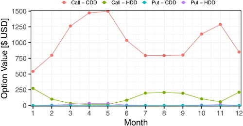
As we expected based on the put-call parity, the put option prices associated with CDDs and the call option prices associated with HDDs move in opposite directions from the call – CDD and call – HDD, respectively.

4. Conclusion

In this paper, a complete framework is developed to value temperature derivatives in equatorial regions. Because there are characteristic changes in temperature for equatorial countries, this task is challenging. Due to the significant differences in temperature patterns in these regions, we address the necessity for a more elaborate DAT model. This model enables us to address a void in the availability of financial instruments to hedge various businesses, ranging from energy generation to entertainment. To achieve this goal, we propose a framework to price the temperature derivatives using a deterministic function with a stochastic process.

Our modeling scheme explored several combinations of different deterministic functions and stochastic processes, which were trained on the same dataset (1961–2011) and later compared on an out-of-sample set (2012–2018) to assess their accuracy. We find that the use of a fourth-order truncated Fourier sum plus a mean-reverting process proves the most accurate in pricing temperature options in Bogotá.

The pricing model uses the Esscher transform to build an appropriate risk-neutral equivalent distribution with which to compute the temperature derivative prices. The market price of risk can vary as a sensibility parameter.

Disclosure statement

No potential conflict of interest was reported by the authors.

Additional information

Notes on contributors

Sergio Cabrales

Sergio Cabrales is an associate professor of Industrial Engineering at Universidad de los Andes, Colombia. He received his PhD in Business Administration at the same university. His research focuses on financial engineering, analytic, game theory, decision analysis applications in the energy sector and financial systems.

Rafael Bautista

Rafael Bautista holds a PhD in management from Tulane University, a PhD in physics from Temple University, and a BSc in physics from Universidad Autónoma de Santo Domingo. His research is in natural resources and financial and economic assessments of artificial systems.

Isabella Madiedo

Isabella Madiedo holds a BSc in engineering from the University of Los Andes. His research interests are data science, machine learning and statistical inference.

María Galindo

María Galindo holds a BSc in engineering from the University of Los Andes. His research interests are data science, machine learning and statistical inference.

References

- Akaike, H. (1974). A new look at the statistical model identification. IEEE Transactions on Automatic Control, 19(6), 716–723. https://doi.org/https://doi.org/10.1109/TAC.1974.1100705
- Alaton, P., Djehiche, B., & Stillberger, D. (2002). On modelling and pricing weather derivatives. Applied Mathematical Finance, 9(1), 1–20. https://doi.org/https://doi.org/10.1080/13504860210132897
- Alexandridis, A., & Zapranis, A. D. (2012). Weather derivatives: Modeling and pricing weather-related risk. Springer Science & Business Media. https://doi.org/https://doi.org/10.1007/978-1-4614-6071-8
- Barrieu, P., & Scaillet, O. (2009). A primer on weather derivatives. In Uncertainty and environmental decision making (pp. 155–175). Springer. https://doi.org/https://doi.org/10.1007/978-1-4419-1129-2_5
- Benth, F. E., & Šaltytė-Benth, J. (2005). Stochastic modelling of temperature variations with a view towards weather derivatives. Applied Mathematical Finance, 12(1), 53–85. https://doi.org/https://doi.org/10.1080/1350486042000271638
- Brockett, P. L., Wang, M., & Yang, C. (2005). Weather derivatives and weather risk management. Risk Management and Insurance Review, 8(1), 127–140. https://doi.org/https://doi.org/10.1111/j.1540-6296.2005.00052.x
- Brockett, P. L., Wang, M., Yang, C., & Zou, H. (2006). Portfolio effects and valuation of weather derivatives. The Financial Review, 41(1), 55–76. https://doi.org/https://doi.org/10.1111/j.1540-6288.2006.00133.x
- Brown, M. E., & Kshirsagar, V. (2015). Weather and international price shocks on food prices in the developing world. Global Environmental Change, 35, 31–40. https://doi.org/https://doi.org/10.1016/j.gloenvcha.2015.08.003
- Cabrera, B. L., Odening, M., & Ritter, M. (2013). Pricing rainfall futures at the CME. Journal of Banking & Finance, 37(11), 4286–4298. https://doi.org/https://doi.org/10.1016/j.jbankfin.2013.07.042
- Campbell, S. D., & Diebold, F. X. (2005). Weather forecasting for weather derivatives. Journal of the American Statistical Association, 100(469), 6–16. https://doi.org/https://doi.org/10.1198/016214504000001051
- Cao, M., & Wei, J. (2000). Pricing the weather. RISK-LONDON-RISK MAGAZINE LIMITED-, 13, 67–70.
- Carr, P., Geman, H., & Madan, D. B. (2001). Pricing and hedging in incomplete markets. Journal of Financial Economics, 62(1), 131–167. https://doi.org/https://doi.org/10.1016/S0304-405X(01)00075-7
- Chantarat, S., Turvey, C. G., Mude, A. G., & Barrett, C. B. (2011). Improving humanitarian response to slow-onset disasters using famine indexed weather derivatives. Agricultural Finance Review, 68(1), 169–195. https://doi.org/https://doi.org/10.1108/00214660880001225
- CME. (2005). An introduction to CME weather products. Retrieved May 3, 2019, from https://www.cmegroup.com/trading/weather/
- Dixit, A. K., Dixit, R. K., & Pindyck, R. S. (1994). Investment under uncertainty. Princeton University Press.
- Dornier, F., & Queruel, M. (2000). Caution to the wind. Energy & Power Risk Management, 13, 30–32.
- Dunis, C. L., & Karalis, V. (2003). Weather derivatives pricing and filling analysis for missing temperature data. Derivative Use Trading Regulation, 9, 61–83.
- Dutton, J. A. (2002). Opportunities and priorities in a new era for weather and climate services. Bulletin of the American Meteorological Society, 83(9), 1303–1312. https://doi.org/https://doi.org/10.1175/1520-0477-83.9.1303
- Elias, M. R. S., Wahab, M., & Fang, L. (2017). Integrating weather and spark spread options for valuing a natural gas-fired power plant with multiple turbines. The Engineering Economist, 62(4), 293–321. https://doi.org/https://doi.org/10.1080/0013791X.2016.1258746
- Escher, F. (1932). On the probability function in the collective theory of risk. Skand. Aktuarie Tidskr, 15, 175–195. https://doi.org/https://doi.org/10.1080/03461238.1932.10405883
- Gerber, H. U., & Shiu, E. S. (1993). Option pricing by Esscher transforms. HEC Ecole des hautes études commerciales.
- Gerber, H. U., & Shiu, E. S. (1996). Actuarial bridges to dynamic hedging and option pricing. Insurance: Mathematics and Economics, 18(3), 183–218. https://doi.org/https://doi.org/10.1016/0167-6687(96)85007-4
- Islip, D., Wei, J. Z., & Kwon, R. H. (2021). Managing construction risk with weather derivatives. The Engineering Economist, 66(2), 150–184. https://doi.org/https://doi.org/10.1080/0013791X.2020.1733721
- Jewson, S., & Brix, A. (2005). Weather derivative valuation: The meteorological, statistical, financial and mathematical foundations. Cambridge University Press. https://doi.org/https://doi.org/10.1198/jasa.2007.s164
- Lee, Y., & Oren, S. S. (2010). A multi-period equilibrium pricing model of weather derivatives. Energy Systems, 1(1), 3–30. https://doi.org/https://doi.org/10.1007/s12667-009-0004-7
- Lucia, J. J., & Schwartz, E. S. (2002). Electricity prices and power derivatives: Evidence from the nordic power exchange. Review of Derivatives Research, 5(1), 5–50. https://doi.org/https://doi.org/10.1023/A:1013846631785
- NOAA. (2018). National oceanic and atmospheric administration. Retrieved September 23, 2018, from https://www.ncdc.noaa.gov
- Rappenglück, B., Schmitz, R., Bauerfeind, M., Cereceda-Balic, F., Von Baer, D., Silva, Y., Rubio, M. A., Lissi, E., & Oyola, P. (2004). An Urban Photochemistry Study in the Metropolitan Region of Santiago de Chile, presented at the 6st Conference on Atmospheric Chemistry: Air Quality in Megacities, 84st Annual Meeting of the American Meteorological Society, Seattle WA/USA, 11 - 15.01.2004
- Schwarz, G. (1978). Estimating the dimension of a model. The Annals of Statistics, 6(2), 461–464. https://doi.org/https://doi.org/10.1214/aos/1176344136
- Seifert, J., & Uhrig-Homburg, M. (2007). Modelling jumps in electricity prices: Theory and empirical evidence. Review of Derivatives Research, 10(1), 59–85. https://doi.org/https://doi.org/10.1007/s11147-007-9011-9
- Spicka, J., & Hnilica, J. (2013). A methodical approach to design and valuation of weather derivatives in agriculture. Advances in Meteorology, 2013, 1–8. https://doi.org/https://doi.org/10.1155/2013/146036
- Swishchuk, A., & Cui, K. (2013). Weather derivatives with applications to Canadian data. Journal of Mathematical Finance, 3(1), 81–95. https://doi.org/https://doi.org/10.4236/jmf.2013.31007
- Turvey, C. G. (2001). Weather derivatives for specific event risks in agriculture. Review of Agricultural Economics, 23(2), 333–351. https://doi.org/https://doi.org/10.1111/1467-9353.00065
- Weber, E. J. (2009). A short history of derivative security markets. In Vinzenz Bronzin’s option pricing models (pp. 431–466). Springer. https://doi.org/https://doi.org/10.1007/978-3-540-85711-2_21
- Xu, W., Odening, M., & Musshoff, O. (2008). Indifference pricing of weather derivatives. American Journal of Agricultural Economics, 90(4), 979–993. https://doi.org/https://doi.org/10.1111/j.1467-8276.2008.01154.x