Long-Horizon Predictability: A Cautionary Tale

Abstract

Long-horizon return regressions effectively have small sample sizes. Using overlapping long-horizon returns provides only marginal benefit. Adjustments for overlapping observations have greatly overstated t-statistics. The evidence from regressions at multiple horizons is often misinterpreted. As a result, much less statistical evidence of long-horizon return predictability exists than is implied by research, which casts doubt on claims about forecasts based on stock market valuations and factor timing.

Disclosure: AQR Capital Management is a global investment management firm that may or may not apply investment techniques or methods of analysis similar to those described herein. The views expressed here are those of the authors and not necessarily those of AQR.

Editor’s Note

Submitted 2 April 2018

Accepted 1 August 2018 by Stephen J. Brown

Pronouncements in the media about how “cheap” or “rich” the stock market or aggregate factor portfolios have become are quite common. These views also creep into the practitioner/academic finance literature:

Evidence of bubbles has accelerated since the crisis. Valuations in the stock and bond markets have reached high levels. . . . 1/CAPE (cyclically adjusted price–earnings) stands at 26, higher than ever before except for the times around 1929, 2000 and 2007, all major market peaks. . . . Long-term investors would be well advised, individually, to lower their exposure to the stock market when it is high, other things equal, and get into the market when it is low. (Shiller 2015, xi, xvi, 204)

Empirical support for these types of statements originates from seemingly “impressive” evidence of the long-horizon predictability of stock returns based on valuation measures. Furthermore, practitioners often document strong levels of statistical significance when analyzing overlapping long-horizon returns based on standard errors that they believe to be correct for overlapping data. (See, among many others, Reichenstein and Rich 1994; Campbell and Shiller 1998; Arnott and Bernstein 2002; Weigand and Irons 2007; Arnott, Beck, Kalesnik, and West 2016; and Siegel 2016.)

The issue is the few independent long-horizon periods in the short samples used to study markets. Using overlapping returns in the hope of increasing the sample size offers little help. Intuitively, no matter how the data are broken down, you can’t get around the issue of small sample sizes. Therefore, findings of long-horizon predictability are illusory and reported statistical significance levels are way off. A quarter-century of statistical theory and analysis of long-horizon return regressions strongly makes this case.¹ The bottom line is that practitioners need to be aware of these issues when performing long-horizon return forecasts and need to appropriately adjust long-horizon statistical metrics.

We show theoretically and demonstrate via simulations that overlapping data for the types of return-forecasting problems faced in finance provide only a marginal benefit. For example, in using 50 years of data to forecast 5-year stock returns, the effective number of observations—from nonoverlapping (10 periods) to monthly overlapping (600 overlapping periods)—increases from 10 to just 12. Statistical significance emerges only because reported standard errors (and t-statistics) are both noisy and severely biased. For example, at the 5-year return horizon with 50 years of data, the range of possible standard error estimates is so wide that inference is nonsensical. The expected t-statistics are effectively double their “true” value. Applying the appropriate statistics to data on long-horizon stock returns and valuation ratios drastically reduces the statistical significance of these tests.

Why Long-Horizon Return Regressions Are Unreliable

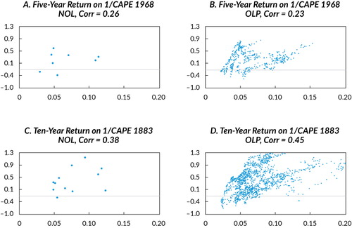
To gain intuition and for illustrative purposes, we provide in Figure 1 the scatterplot of the inverse of the cyclically adjusted price-to-earnings ratio (1/CAPE) and subsequent 5-year stock returns post-1968 (nonoverlapping in Panel A) and 10-year stock returns post-1883 (nonoverlapping in Panel C). Note that the numbers of nonoverlapping observations are 8 and 12, respectively. The point estimates of the correlations are quite large and positive, 0.26 and 0.38. Very few data, however, back up these estimates. For example, suppose one were to take away the farthest outlier point in the plot; then, the correlations become, respectively, 0.04 and 0.28. Of course, this finding should not be a surprise. Under the null of no predictability, and putting aside any bias adjustment, the standard error of the correlation coefficient is $1/\sqrt{T}$, which is 0.35 for 8 observations and 0.29 for 12 observations. In other words, the true correlation may quite possibly be zero or negative, especially for 5-year stock returns used in the late subsample.

Figure 1. Forecasting Stock Returns Using 1/CAPE

Note: NOL = nonoverlapping; OLP = overlapping; Corr = correlation.

In an attempt to combat this issue, practitioners, believing they are increasing their sample sizes significantly, often sample long-horizon stock returns more frequently by using overlapping observations. For example, in referring to 1/CAPE’s ability to forecast 10-year returns relative to his previous work, Shiller (2015) wrote in the latest edition of his book Irrational Exuberance,

We now have data from 17 more years, 1987 through 2003 (end-points 1997 through 2013), and so 17 new points have been added to the 106 (from 1883). (204)

Consistent with this observation, the overlapping scatterplots on the right-hand side of Figure 1 are in stark contrast to those on the left-hand side and appear to show overwhelming evidence of a strong positive relationship. As such, in describing this estimated positive relationship between 1/CAPE and future long-term returns, Shiller (2015) wrote “the swarm of points in the scatter shows a definite tilt” (204).

This appearance is fallacy.² In Shiller’s example, because 1/CAPE (measured as a 10-year moving average of earnings) is highly persistent, only 2—not 17—nonoverlapping observations have been truly added. To see this fact, note that standing in January 2003 and in January 2004 and looking ahead 10 years in both cases, the future 10-year returns have 9 years in common. So, even if stock returns are serially independent through time, the 10-year returns in adjacent years will be 0.90 correlated by construction. Moreover, 1/CAPE itself has barely changed because of its 10-year moving average of earnings and the fundamental persistence of stock prices during the period between January 2003 and January 2004. It is these facts that create, by construction, Shiller’s “swarm” effect visible in Panels B and D of Figure 1. In reality, we have simply a smattering of independent data points—12, to be precise. How much, if at all, do overlapping observations really benefit the practitioner?

Formally, a typical long-horizon regression involves regressing J-period horizon returns of an asset, $R_{t:t+J}$, on some lagged predictive variable, $X_t,$ using T periods of data:

$R_{t:t+J}={\alpha }_J+{\beta }_J{X}_t+{\epsilon }_{t:t+J}.$ (1)

In the context of this article, $X_t$ is usually some price-based measure of valuation of the underlying asset or factor, such as Shiller’s market 1/CAPE, the current dividend yield of the market, the value spread of a factor, or a contrarian view on the asset (e.g., the asset’s past J-period return horizon).

If the practitioner does not use overlapping return data and samples the data every J periods, the number of observations is T/J and standard textbook ordinary least squares (OLS) regression applies. If J is large relative to T, then the practitioner has only a few observations and the standard errors will be generally too large to infer the true ${\beta }_J$. This outcome is especially true for stock returns because the expected-return component has a relatively small variation relative to realized returns (see, e.g., Elton 1999).

As a potential solution to T/J being small, practitioners can sample more frequently. On one level, this technique makes sense: Using all the data will improve efficiency. For using persistent regressors to forecast stock returns, however, the efficiency gains will be minor. To understand this claim, suppose we want to forecast five-year return horizons from 1968 to 2016. We could choose 8 nonoverlapping five-year-long observations or 44 annually sampled five-year returns or, perhaps better, 528 monthly, 2,288 weekly, or 11,440 trading day–sampled five-year returns. At first glance, this increase seems to hold the promise of adding a lot of information, allowing us to move from, say, a sample size of 8 to one of 11,440. The problem is that five-year returns from one day to the next have 1,249/1,250 (i.e., 99.92%) of the data in common. If the $X_t$ variable also does not change from one day to the next, as is common when using such valuation ratios as 1/CAPE or long-lookback contrarian strategies, then both the left-hand and right-hand sides of regression Equation 1$R_{t:t+J}={\alpha }_J+{\beta }_J{X}_t+{\epsilon }_{t:t+J}.$ (1) are the same over contiguous time periods.

To illustrate this point, we report in Figure 2 the simulated distribution of the coefficient estimators for the J-period return regression in Equation 1$R_{t:t+J}={\alpha }_J+{\beta }_J{X}_t+{\epsilon }_{t:t+J}.$ (1) with data matched to 1/CAPE under the model assumption of no predictability.³ Figure 2 shows box plots of the 5%, 25%, 50%, 75%, and 95% values of the simulated distribution of the coefficient estimators for the J-period return regression in Equation 1$R_{t:t+J}={\alpha }_J+{\beta }_J{X}_t+{\epsilon }_{t:t+J}.$ (1) . The predictive variable, $X_t$, is assumed to follow an AR(1) with autocorrelation parameter 0.991 to match the persistence of monthly observed 1/CAPE.

Figure 2. Simulated Distribution of Long-Horizon Coefficient Estimators

Notes: The estimators are compared by using overlapping observations versus nonoverlapping observations and assuming 50 years (600 months) of data and monthly sampling. The black box plots (right) represent the nonoverlapping cases; the green box plots (left) represent the overlapping cases.

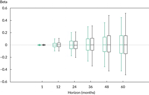
The distribution of the coefficient estimator for the nonoverlapping regression (in black) widens greatly as the horizon increases from J = 1 to J = 60. That is, as the return horizon lengthens, the chance of observing betas far from the true value of 0.0 greatly increases. This result is not at all surprising because the number of observations decreases from 600 to 10. Consistent with this intuition, however, Figure 2 shows that the distribution of the estimators using overlapping observations (in green) is not much tighter than the nonoverlapping case; that is, the distributions are basically the same. This fact poses a significant inference problem for practitioners trying to forecast large J-period return horizons because they have effectively few observations. In other words, using overlapping observations for persistent regressors provides little benefit.

Figure 2 plots the distribution of the regression coefficients under the null hypothesis of no predictability (with persistent regressors) and demonstrates that lack of benefit from overlapping observations. A practitioner might have a prior belief, however, that stock returns are predictable. How would this prior belief change the practitioner’s view of the observed coefficient estimators?

Figure 3 compares the simulated distribution of the predictability coefficient from 60-month return regressions and nonoverlapping and overlapping data under the assumption of no predictability (as in Figure 2) with the distribution of predictability under the assumption that the true coefficient value equals the ex post in-sample value.

Figure 3. Simulated Distribution of Long-Horizon Coefficient Estimator: No Predictability (right) vs. Predictability of Returns (left)

Table

%-tile	b(Null)	b(Alt)
0.010	–0.783	–0.630
0.050	–0.426	–0.272
0.100	–0.316	–0.160
0.250	–0.155	0.011
0.500	0.005	0.172
0.750	0.176	0.339
0.900	0.360	0.517
0.950	0.447	0.612
0.990	0.689	0.816

Notes: The predictive variable X_t is assumed to follow an AR(1) with autocorrelation parameter 0.991 to match the persistence of monthly observed 1/CAPE, and the alternative distribution uses the in-sample regression coefficient estimate as the true value. The 50 years (600 months) of nonoverlapping (overlapping) 5-year return data were used. Note that the black lines represent the predictability case and the green lines represent the no-predictability case.

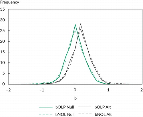
Note first that shifting from no predictability to predictability does not change the message that overlapping observations provide little benefit. The distributions of the coefficient estimators are still on top of each other (black on dashed black, green on dashed green). Equally important is that the no-predictability distribution is quite similar to the alternative predictability-assumed distribution, with only a slight shift to the right (the black versus green lines). For example, the 5% and 95% tails of the null and alternative distributions are, respectively, –0.43 versus –0.27 and 0.45 versus 0.61. That said, a practitioner with strong convictions might find some comfort in the fact that the distribution of the regression coefficient under predictability does suggest, albeit weakly, a higher probability of observing predictability than no predictability.

Why Long-Horizon Return Regressions Are Unreliable: Theory

The preceding intuition can be couched in terms of formal statistical theory. In estimating Equation 1$R_{t:t+J}={\alpha }_J+{\beta }_J{X}_t+{\epsilon }_{t:t+J}.$ (1) , the practitioner can use nonoverlapping data and use the OLS standard errors (denoted as “nol”). Alternatively, the practitioner can use overlapping data and estimate regression Equation 1$R_{t:t+J}={\alpha }_J+{\beta }_J{X}_t+{\epsilon }_{t:t+J}.$ (1) but, in this case, adjust the asymptotic variance of the ${\beta }_J$ estimator for serial dependence in the OLS errors resulting from the overlap (the overlapping estimator denoted as “ol”). Under the maintained hypothesis of no predictability (i.e., ${\beta }_J=0$), the practitioner can directly compare the variances of the estimators for nonoverlapping versus overlapping data:⁴$$\mathrm{var}\left({\widehat{\beta }}_J^{ol}\right)=\mathrm{var}\left({\widehat{\beta }}_J^{nol}\right)\left[\frac{1}{J}+\theta \left(J,{\rho }_J\right)\right],$$ (2) where $\theta \left(J,{\rho }_J\right)=2{\displaystyle {\sum }_{j=1}^{J-1}\left[\left(J-j\right)/J^2\right]}{\rho }_j$and ${\rho }_j$ is the jth-order autocorrelation of $X_t.$

Equation 2$$\mathrm{var}\left({\widehat{\beta }}_J^{ol}\right)=\mathrm{var}\left({\widehat{\beta }}_J^{nol}\right)\left[\frac{1}{J}+\theta \left(J,{\rho }_J\right)\right],$$ (2) is intuitively appealing. In comparing the variance of the estimators, the first term in the brackets in Equation 2$$\mathrm{var}\left({\widehat{\beta }}_J^{ol}\right)=\mathrm{var}\left({\widehat{\beta }}_J^{nol}\right)\left[\frac{1}{J}+\theta \left(J,{\rho }_J\right)\right],$$ (2) , 1/J, reflects the fact that the ol estimator has J times the observations of the nol estimator and, on the surface, 1/Jth the variance. This observation is the reason so many practitioners use regression methodologies based on overlapping data. The second term in the bracket in Equation 2$$\mathrm{var}\left({\widehat{\beta }}_J^{ol}\right)=\mathrm{var}\left({\widehat{\beta }}_J^{nol}\right)\left[\frac{1}{J}+\theta \left(J,{\rho }_J\right)\right],$$ (2) , however, $\theta \left(J,{\rho }_J\right)$, represents the upward adjustment that needs to be made to the ol estimator’s variance because of the length of the overlap, J, and persistence of predictive variable $X_t,$ ${\rho }_1\dots {\rho }_J$. Unfortunately, if $X_t$ is highly persistent (say, ${\rho }_j$ is close to 1), then the variance of the ol estimator is the same as that of the nol estimator and no efficiency is gained.⁵

The problem is that in most practical applications, the predictor exhibits high persistence (e.g., current valuation ratios such as 1/CAPE and the dividend-to-price ratio, or five-year lagged stock returns). All of these do not change much from month to month. For instance, consider 1/CAPE’s value from month to month. The variable 1/CAPE represents a 10-year moving average of earnings over a highly persistent price series, both of which show little variation from month to month. Thus, 1/CAPE’s autocorrelation is close to 1.0 and zero efficiency gain comes from increasing the sampling frequency. To pin down this point, Equation 2$$\mathrm{var}\left({\widehat{\beta }}_J^{ol}\right)=\mathrm{var}\left({\widehat{\beta }}_J^{nol}\right)\left[\frac{1}{J}+\theta \left(J,{\rho }_J\right)\right],$$ (2) can be translated into an equivalent number of observations that would provide the same asymptotic standard errors when comparing overlapping versus nonoverlapping regressions. Specifically, we can calculate Equation 2$$\mathrm{var}\left({\widehat{\beta }}_J^{ol}\right)=\mathrm{var}\left({\widehat{\beta }}_J^{nol}\right)\left[\frac{1}{J}+\theta \left(J,{\rho }_J\right)\right],$$ (2) by assuming $X_t$ follows an AR(1) process with autoregressive parameter ${\rho }_X$ and then ask how many more nonoverlapping observations we would need to equate the ol and nol cases. Table 1 provides the results.

Table 1. Equivalent Number of Observations for Overlapping vs. Nonoverlapping Data

			Effective Number of Nonoverlapping Observations for Overlapping Data
T	J	Nonoverlapping Observations	${\rho }_x$ = 0.0	${\rho }_x$ = 0.971	${\rho }_x$ = 0.991	Contrarian
600	1	600	600	600	600	600
600	12	50	600	56	52	75
600	24	25	600	31	27	37
600	36	17	600	23	18	25
600	48	13	600	19	14	19
600	60	10	600	17	12	15
600	120	5	600	12	7	8

Notes: J = 12-, 24-, 36-, 48-, 60-, and 120-period return forecasts with 50 years of data, monthly sampling. Values of ${\rho }_X$ coincide with typical levels of persistence observed empirically—namely, 0.991 = 0.90^1/12 for monthly 1/CAPE and 0.971 = 0.70^1/12 for VALUE (the value spread of the value factor).

The way to read the table is as follows. For the ${\rho }_X=0.991$ column, relevant for 1/CAPE, the effective increase in observations (going from nonoverlapping to overlapping) for the 12-month forecasting horizon is from 50 nonoverlapping observations to an equivalent of monthly overlap of 52 observations; for 24 months, from 25 to 27 observations; for 36 months, from 17 to 18 observations; for 48 months, from 13 to 14 observations; for 60 months, from 10 to 12 observations; and for the 120-month forecasting horizon, from 5 independent observations to an equivalent in statistical terms of 7 observations. That is, although using overlapping observations at longer horizons provides increasing efficiency gains, longer horizons also unfortunately substantially reduce the number of nonoverlapping observations. In other words, the effective increase in the number of observations when using overlapping data is too small to have any real impact on one’s ability to predict long-horizon returns.

Why Standard Error Procedures for Long-Horizon Return Regressions Are Inaccurate

The preceding results are bad news for practitioners relying on long-horizon predictability to distinguish between no predictability and a market-timing view of the world. With long-horizon returns and persistent regressors, the type used commonly in return forecasts, almost no benefit comes from using overlapping observations. Note that one cannot sidestep the small sample size—that is, Figure 2 does not lie.

This conclusion may come as a surprise to practitioners, who commonly estimate long-horizon returns and document so-called predictability. When performing these long-horizon tests, however, practitioners invariably are provided false comfort by estimating standard errors in the presence of overlapping observations common in statistical packages.⁶ In this section, we consider the method most used by practitioners for correcting for overlapping observations—namely, the method of Newey and West (1987). The popularity of the Newey–West approach results from the fact that it offers a feasible standard error estimate in small samples and yet is theoretically justified in asymptotic terms. The problem is that the Newey–West procedure was never meant to be used for large J relative to T.

The reason is multifold. First, the assumed weighting scheme for the Newey–West approach is inconsistent with the theoretical lag structure implied by Equation 2$$\mathrm{var}\left({\widehat{\beta }}_J^{ol}\right)=\mathrm{var}\left({\widehat{\beta }}_J^{nol}\right)\left[\frac{1}{J}+\theta \left(J,{\rho }_J\right)\right],$$ (2) and underestimates the true standard error. Second, Newey–West standard errors require estimates of the autocovariance of the residuals from the OLS normal equations $\left(\widehat{{\epsilon }_{t,t+J}}\text{ and }\widehat{{\epsilon }_{t,t+J}}{X}_t\right)$ across multiple lags in Equation 1$R_{t:t+J}={\alpha }_J+{\beta }_J{X}_t+{\epsilon }_{t:t+J}.$ (1) . A well-known negative bias is associated with autocorrelation estimators, however (e.g., see Kendall 1954), and this bias increases dramatically for small sample sizes.⁷ Third, the Newey–West standard errors are themselves noisy estimators for large J relative to T for the reasons given previously. In other words, estimation bias aside, the standard error estimates are unreliable.

To illustrate these points, Figure 4 reports simulations of Newey–West standard errors (box plots in green) and, for comparison purposes, Hansen–Hodrick standard errors (box plots in black) under assumptions underlying returns and regressors chosen to match the persistence properties of $X_t$ discussed earlier.⁸

Figure 4. Simulated Distribution of Newey–West and Hansen–Hodrick Standard Errors

Notes: The distributions of the standard errors are provided at the 5%, 25%, 50%, 75%, and 95% levels for horizons 1, 12, 24, 36, 48, and 60 with T = 600 (i.e., J-period return horizon and 50 years of data) and AR(1) parameter to match the monthly 1/CAPE series, ρ_{x =} 0.991. For each horizon, the theoretical analytical asymptotic standard error is denoted by a dot, and the green and black box plots represent, respectively, Newey–West and Hansen–Hodrick standard errors.

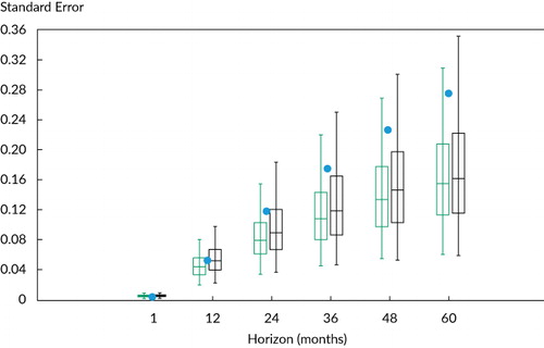
In Figure 4, the underestimate of Newey–West standard errors relative to the analytical ones can be seen clearly in the plot, which also shows that this bias increases with horizon J. Specifically, for J = 12, 24, 36, 48, and 60, the ratio of the average Newey–West standard error to the true analytical value declines to, respectively, 0.718, 0.671, 0.626, 0.588, and 0.553. The increasing bias seen in Figure 4 partially explains why practitioners so often find evidence of predictability only at long horizons. The true analytical standard errors increase with the horizon. Because of the various biases, however, the Newey–West standard errors level off more quickly. In fact, for J = 60, the t-statistics are inflated by 81% (1/0.553).

To dig a little deeper into the accuracy of Newey–West t-statistics, Panel A in Table 2 provides the simulated Newey–West t-statistics together with theoretical t-statistic values at p-values ranging from 1% to 99%.⁹ Consistent with Figure 4, the most notable finding is that the t-statistics are upward biased (in absolute magnitude) and become progressively worse with a lengthening horizon. For example, consider the 2.5% p-value’s standard t-statistic of –1.96. The corresponding Newey–West t-statistics are –2.67, –2.94, –3.19, –3.67, and –3.98, respectively, at horizon lengths of 12, 24, 36, 48, and 60 months. Thus, at long horizons (i.e., J = 60), the t-statistics are effectively double. Panel B in Table 2 provides a related perspective. The table reports the p-values at the standard t-statistic levels. The second row corresponds to the theoretical p-value ranges, whereas the actual simulated p-values using Newey–West are reported in the other rows for different horizons. These rows show that the practitioner believes he is making a mistake only 2.5% of the time but is actually making an error much more frequently. For example, using the t-statistic value of –1.96 at an assumed 2.5% p-value rate of rejection leads to excess rejection rates of 6.6%, 7.3%, 9.5%, 10.6%, and 12.1% at horizon lengths of 12, 24, 36, 48, and 60 months.

Table 2. The Distribution of Newey–West t-Statistics

A. Simulated Newey–West t-statistics
Percentile	1.0	2.5	5.0	10.0	90.0	95.0	97.5	99.0
Normal	–2.32	–1.96	–1.65	–1.28	1.28	1.65	1.96	2.33
Horizon (months)
1	–2.41	–2.08	–1.71	–1.28	1.32	1.66	1.93	2.27
12	–3.36	–2.67	–2.15	–1.64	1.80	2.42	2.68	3.15
24	–3.63	–2.94	–2.35	–1.73	1.94	2.65	3.23	3.72
36	–4.02	–3.19	–2.64	–1.91	2.04	2.87	3.41	4.02
48	–4.70	–3.67	–2.89	–2.01	2.15	2.93	3.63	4.24
60	–4.76	–3.98	–3.05	–2.21	2.25	3.02	3.73	4.75
B. Simulated Newey–West p-values based on standard t-statistic levels
Statistic	–2.32	–1.96	–1.65	–1.28	1.28	1.65	1.96	2.33
Normal	1.0	2.5	5.0	10.0	90.0	95.0	97.5	99.0
Horizon (months)
1	1.4	3.2	5.4	9.8	89.1	94.8	97.5	99.0
12	3.7	6.6	9.8	14.1	83.1	87.9	91.6	94.7
24	5.0	7.3	10.8	16.3	82.3	87.1	90.3	93.1
36	6.2	9.5	12.7	17.8	81.2	86.0	89.3	92.0
48	8.2	10.6	14.0	19.7	79.4	84.8	88.3	91.3
60	8.5	12.1	15.0	20.4	77.5	83.7	87.6	90.5

As problematic as these results are for using Newey–West standard errors, they only partially tell the story. An equally important observation from Figure 4 is how noisy the standard error estimates are and how this condition worsens with the lengthening of the horizon. For example, consider calculating the standard deviation of the range of standard errors at each J-period horizon in Figure 4. Relative to the simulated mean standard errors of 0.063, 0.120, 0.176, 0.228, and 0.275 at, respectively, J = 12, 24, 36, 48, and 60, the corresponding standard deviations of the Newey–West standard error distribution are 0.019, 0.038, 0.056, 0.071, and 0.083. Note that the standard deviation increases with the horizon at basically the same rate as the level of the standard errors themselves. We should have little faith, therefore, in the accuracy of Newey–West standard errors for large J relative to the T seen in practice.

Empirical Application

Empirical evidence of stock market return predictability at short horizons is weak (e.g., see Welch and Goyal 2008).¹⁰ This weakness is one of the reasons practitioners focus on long-horizon predictability. In this section, we consider forecasts of long-horizon stock market returns using 1/CAPE and factor returns— HML (high book to market minus low book to market) for value and MOM for momentum. We use the value spreads of these factors. Value-spread timing provides a potentially interesting contrast to 1/CAPE because value spreads are less persistent. Note that we consider return data for 1968–2016 to coincide with popular sample sizes found in the practitioner literature, but we also consider the longer sample of 1/CAPE going back to 1883.

Table 3 reports the coefficient estimate and R² of the J-period return regression given in Equation 1$R_{t:t+J}={\alpha }_J+{\beta }_J{X}_t+{\epsilon }_{t:t+J}.$ (1) starting from 1968 and using monthly overlapping data (and from 1883 for the long-sample 1/CAPE regression). We report the typical Newey–West standard errors, the derived theoretical standard errors, and the simulated p-value (under the null hypothesis of no predictability with AR[1] regressor to match the data). These p-values represent the location of the estimated β_J coefficient in the range of the simulated distribution.¹¹ Joint tests across the horizons are also provided (e.g., see Boudoukh, Richardson, and Whitelaw 2008).

Table 3. Empirical Results for Long-Horizon Predictability

	Horizon
	1	12	24	36	48	60	Joint Test Simulated p-Value
HML on value spread, N = 525, ρX = 0.972
β	0.003	0.047	0.091	0.126	0.153	0.168
N–W t-stat.	1.159	2.718	5.477	4.272	4.142	4.476
AR(1) t-stat.	2.125	2.992	3.062	2.950	2.831	2.588	0.074
Simulated p-value	0.082	0.020	0.010	0.007	0.009	0.009	0.110
R^2	0.860	14.450	26.382	34.191	38.521	38.789
MOM on value spread, N = 525, ρX = 0.917
β	0.013	0.141	0.125	0.151	0.215	0.204
N–W t-stat.	1.839	2.498	2.116	1.962	2.199	2.123
AR(1) t-stat.	1.957	2.109	1.070	0.968	1.136	0.938	0.107
Simulated p-value	0.037	0.026	0.170	0.190	0.138	0.181	0.131
R^2	0.730	7.519	4.366	5.376	8.513	6.878
	1	24	48	72	96	120
Market on 1/CAPE 1883, N = 1,510, ρX = 0.990
β	0.091	2.458	4.590	5.841	7.083	7.569
N–W t-stat.	1.729	2.504	2.576	3.745	4.884	3.541
AR(1) t-stat.	2.192	2.562	2.482	2.181	2.053	1.813	0.090
Simulated p-value	0.116	0.061	0.054	0.063	0.061	0.091	0.117
R^2	0.318	7.876	15.089	18.957	22.392	20.094
	1	12	24	36	48	60
Market on 1/CAPE 1968, N = 528, ρX = 0.993
β	0.065	0.909	1.452	1.628	2.045	2.850
N–W t-stat.	0.896	1.279	1.154	0.980	1.107	1.526
AR(1) t-stat.	0.940	1.107	0.896	0.678	0.647	0.731	0.222
Simulated p-value	0.569	0.517	0.576	0.656	0.662	0.639	0.364
R^2	0.167	2.292	2.986	2.766	3.411	5.269

Note: Joint statistical tests across the horizons (using theoretical analytical calculations and simulated p-values) are provided in the last column.

Consider the 1/CAPE regression from 1883. As reported elsewhere, the coefficients and R²s (e.g., 22.4% and 20.1% at 5 years and 10 years) are large and generally increase with the return horizon. The t-statistics when Newey–West standard errors are used range between 3.5 and 4.9 at longer horizons. As we argued earlier, these results can be deceiving. Indeed, even though the 1/CAPE regression is arguably the best-known example of predictability, the t-statistics for the analytical standard errors are much smaller, hovering around 2, and the simulated p-values are around 10% across the horizons. In other words, more positive coefficient estimates are observed approximately 10% of the time when simulated data are used with no predictability. This finding borders on statistical significance but is far away from the huge t-statistics (and associated p-values) found when using Newey–West. In addition, when applying a joint test across horizons (e.g., Boudoukh et al. 2008), the evidence weakens. In other words, the fact that predictability “shows up” at many horizons is more consistent with the high correlation across the estimators than any proof of statistical significance.

Many of the Newey–West-inspired t-statistics are greater than 2 for long horizons for both 1/CAPE post-1968 and factor-timing variables, but the evidence is considerably weaker for theoretical t-statistics or simulated p-values. An exception is HML spread, which is significant at standard levels irrespective of the standard error methodology. Note that greater benefit comes from using overlapping data because HML is less persistent (i.e., AR[1] of 0.972 versus 0.993 for 1/CAPE). That said, this result also disappears with a joint test across horizons.¹² In any event, aside from this predictive variable, less evidence exists for long-horizon return predictability than is implied by existing research.

Practical Suggestions

What choices does the practitioner have when performing long-horizon forecasts facing this long-horizon, small-sample issue?

First and foremost, the practitioner should not use the type of standard error adjustments implied by Newey and West (1987), among others, because of the adjustments’ severe downward bias. Instead, Equation 2$$\mathrm{var}\left({\widehat{\beta }}_J^{ol}\right)=\mathrm{var}\left({\widehat{\beta }}_J^{nol}\right)\left[\frac{1}{J}+\theta \left(J,{\rho }_J\right)\right],$$ (2) of this article provides the appropriate analytical standard error, which is simply a function of the nonoverlapping standard error and the autocorrelogram of the predictive variable. Importantly, Figure 4 shows that the Newey–West and Hansen–Hodrick standard errors are highly variable because of the many parameters required in estimation. The advantage of the analytical approach is that many fewer parameters need to be estimated. In fact, if the practitioner is willing to specify an autoregressive process for the predictive variable, the autocorrelogram will be a function of only a few parameters (see note 4). For different justifications, Valkanov (2003) and Hjalmarsson (2011) suggested simply calculating the usual t-statistic but then scaling it down by $\sqrt{J}$. Note that this approach is quite conservative; it is equivalent to Equation 2$$\mathrm{var}\left({\widehat{\beta }}_J^{ol}\right)=\mathrm{var}\left({\widehat{\beta }}_J^{nol}\right)\left[\frac{1}{J}+\theta \left(J,{\rho }_J\right)\right],$$ (2) with all the autocorrelation parameters, ${\rho }_j\left(j=1,\dots ,J\right)$, set equal to 1.0. Nevertheless, multiplying the OLS standard error by $1/\sqrt{J}$ is at least preferable to current uses of Newey–West standard errors.

Second, in the empirical application (see Table 3), we performed joint tests across the horizons. For a given horizon, similar joint tests can be performed for various assets (e.g., see Richardson 1993). These joint tests potentially increase the power to detect long-horizon predictability, effectively increasing the sample size. This effective increase depends on how the pattern in coefficient estimates for the assets relates to the contemporaneous correlation across the asset returns. In addition, to the extent that the long-horizon forecasts behave similarly among assets, the researcher can pool the asset return regressions to effectively increase the sample size. Indeed, although the studies of Hjalmarsson (2010) and Lawrenz and Zorn (2017) were not focused on long horizons, both documented similar patterns across assets for using valuation ratios to predict stock returns. They documented stronger statistical evidence when pooling the regression equations to estimate the coefficient. Note that there is an analytical standard error analogous to that of Equation 2$$\mathrm{var}\left({\widehat{\beta }}_J^{ol}\right)=\mathrm{var}\left({\widehat{\beta }}_J^{nol}\right)\left[\frac{1}{J}+\theta \left(J,{\rho }_J\right)\right],$$ (2) for pooled regressions, although it also includes the correlation matrix across asset returns.

Third, the message of this article is bad news for contrarians and market timers who rely on long-horizon evidence to make their case. Apparent predictability is illusory or, at least, consistent with the null hypothesis of no market timing. Of course, a researcher may have a prior belief that low-frequency persistence in factors leads to slow mean reversion in stock prices (either risk based or behavior based), generating large amounts of predictability only at long horizons (see Cochrane 2008). The data will likely confirm this belief. The point here is that this evidence does not really help differentiate between the null hypothesis of no predictability and this alternative prior belief (see Figure 3). An interesting paper by Lamoureux and Zhou (1996) effectively confirmed this point by applying a formal Bayesian analysis to random walk tests of long-horizon returns. That said, rethinking long-horizon predictability in a Bayesian setting may provide a more even-handed view of the evidence.

Fourth, when a researcher lacks the effective sample size to generate efficient estimates, the typical solution is for the researcher to build more structure into the estimation problem. Examples in the literature of such an approach are Lewellen (2004); Campbell and Yogo (2006); Campbell and Thompson (2008); and Cochrane (2008)—all of whom took into account the joint distribution of asset returns and valuation ratios in some economic or statistical model. As an illustration, consider Cochrane. Using the dividend discount model, Cochrane pointed out that dividend yield predictability must be related to either dividend growth or return predictability, and he used the lack of dividend growth predictability to generate tight estimates of stock return predictability (see also Leroy and Sinhania 2018). This approach shows promise and provides a viable way of generating long-horizon return forecasts. Of course, the success or failure depends greatly on the assumed underlying model and estimation.¹³

Finally, given the existence of short-horizon predictability (as documented in, e.g., Lewellen 2004; Campbell and Yogo 2006; Campbell and Thompson 2008), a potentially efficient methodology would be to model the short-horizon structure of the predictive variable and infer long-horizon forecasts from this imposed structure. In the case of long-horizon return regressions, this strategy suggests joint estimation of a short-horizon return process and autoregressive process for the predictive variable. Given such joint estimation of $\left(R_{t,t+1},X_t\right)$ based on $\left(X_{t-1},\dots ,X_{t-m}\right)$, where m is small relative to J, the researcher can infer a long-horizon J-period return forecast. (See, e.g., Kandel and Stambaugh 1989; Campbell 1991; Hodrick 1992; Boudoukh and Richardson 1994; and Campbell, Lo, and MacKinlay 1997.)

To see how this approach works, consider the estimation problem at one-period horizons with the assumption that the predictive variable, $X_t$, follows an AR(1) with parameter ${\rho }_X$. For illustrative purposes, this model is the same example covered in the preceding sections. Specifically,$R_{t:t+1}={\alpha }_1+{\beta }_1{X}_t+{\epsilon }_{t:t+1},$ $X_{t+1}=\mu +{\rho }_X{X}_t+{\eta }_{t+1}.$ (3) Now, suppose we estimate Equation 3$X_{t+1}=\mu +{\rho }_X{X}_t+{\eta }_{t+1}.$ (3) jointly and use the estimates to generate a forecast for $R_{t,t+j}$; that is, we estimate ${\beta }_J$ (in Equation 1$R_{t:t+J}={\alpha }_J+{\beta }_J{X}_t+{\epsilon }_{t:t+J}.$ (1) ) from ${\beta }_1$ and ${\rho }_X$. Boudoukh and Richardson (1994) showed that a consistent estimator is ${\beta }_J^{imp}={\beta }_1\left[\left(1-{\rho }_X^J\right)/\left(1-{\rho }_X\right)\right],$ where imp refers to the J-period estimator implied from the nonlinear function of ${\beta }_1$ and ${\rho }_X$. No issue of overlapping error interferes here, and the variance of ${\widehat{\beta }}_J^{imp}$ is simply the OLS estimator, $\left[\mathrm{var}\left(R_t\right)/\mathrm{var}\left(X_t\right)\right]\left[{\left((1-{\rho }_X^J)/(1-{\rho }_X)\right)}^2\right]$. This variance is magnitudes lower than the overlapping and nonoverlapping multiperiod estimators derived in Equation 2$$\mathrm{var}\left({\widehat{\beta }}_J^{ol}\right)=\mathrm{var}\left({\widehat{\beta }}_J^{nol}\right)\left[\frac{1}{J}+\theta \left(J,{\rho }_J\right)\right],$$ (2) . The intuition is that we estimate monthly βs well and use up only one degree of freedom when we estimate ${\rho }_X$.

Of course, there is no free lunch. Two problems, in particular, stand out. The first problem is that the estimator will be inconsistent if the model is wrong. To improve the consistency, we need to build a more complex model, but a more complex model introduces more and more estimation error. The second problem is that any biases that exist in estimation—and we know from Kendall (1954) and Stambaugh (1993, 1999) that biases exist for our forecasting problem—will be amplified because the inferred ${\beta }_J$ is a nonlinear function of ${\beta }_1$ and ${\rho }_X$. Indeed, although the potential benefits in efficiency gains are large and represent a solution to the long-horizon predictability problem, the evidence is somewhat mixed. For example, see the conclusions reached by Bekaert and Hodrick (1992) versus those of Neely and Weller (2000).

Conclusion

By construction, long-horizon return regressions have effectively small sample sizes. As a remedy, practitioners use more frequent sampling of the long-horizon returns to perform these regressions. We showed that the benefit of using overlapping observations is marginal because the predictive variable tends to be highly persistent. Standard statistical packages that calculate t-statistics based on adjustments for overlapping observations do not help; in fact, they tend to inflate the t-statistics. Researchers should be aware of these issues to avoid drawing incorrect inferences.

We offered an analytical approach to account for these known biases, and we suggested that some promise may be found in running joint tests for different assets, having economic priors and updating them in a Bayesian setting, and adding structure to the estimation problem.

Acknowledgments

We would like to thank Stephen J. Brown, Daniel Giamouridis, and two anonymous reviewers. We would also like to thank Cliff Asness, Esben Hedegaard, Antti Ilmanen, Bryan Kelly, Toby Moskowitz, and Lasse Pedersen for helpful comments and suggestions.

Notes

¹ The history in finance of studying the statistics of long-horizon regressions is extensive. For general applications, see Hansen and Hodrick (1980); Newey and West (1987); Richardson and Smith (1991); Andrews (1991). For applications to return predictability, see Richardson and Stock (1989); Hodrick (1992); Richardson (1993); Nelson and Kim (1993); Goetzmann and Jorion (1993); Boudoukh and Richardson (1994); Valkanov (2003); Boudoukh, Richardson, and Whitelaw (2008); Hjalmarsson (2011); Britten-Jones, Neuberger, and Nolte (2011); Kostakis, Magdalinos, and Stamatogiannis 2015. All of these methods provide ways to correct for the inference problem in a framework of overlapping errors.

² Asness, Ilmanen, and Maloney (2017) discussed the issues related to valuation-based long-horizon regressions from a more practical perspective. They contrasted the visually appealing relationship between starting valuations and next-decade realized market returns against the disappointing economic gains achieved by market-timing trading rules based on time-varying valuations. They further explained mechanically why, given the apparent statistical evidence of predictability, such contrarian market-timing strategies have not outperformed the buy-and-hold portfolio over the past half-century.

³ For illustrative purposes, in the simulations to follow, we assumed that the predictive variable, X_t, follows a first-order autoregressive process [AR(1)] with parameters corresponding to those of 1/CAPE. We know that the innovations in AR processes for such valuation ratios as 1/CAPE and stock returns are contemporaneously correlated, which leads to a bias toward predictability (see, e.g., Stambaugh 1993, 1999). So as not to conflate the overlapping versus nonoverlapping focus of this article, we assumed in our simulations that this correlation is zero. That said, for robustness, we confirmed similar findings for Figure 2 under different contemporaneous correlation assumptions matched to the data. Of particular importance is that all the results and implications followed similarly. An interesting finding (not pursued here) is that the predictability bias worsened as the horizon increased (see also Nelson and Kim 1993; Torous, Valkanov, and Yan 2004). Note that the simulated p-values for the actual empirical applications in a later table do incorporate the nonzero contemporaneous correlation.

⁴ See Boudoukh and Richardson (1994) and Boudoukh et al. (2008). For particular assumptions about the autoregressive process for $X_t$, Equation 2$$\mathrm{var}\left({\widehat{\beta }}_J^{ol}\right)=\mathrm{var}\left({\widehat{\beta }}_J^{nol}\right)\left[\frac{1}{J}+\theta \left(J,{\rho }_J\right)\right],$$ (2) can be written analytically. For example, assuming $X_t$ follows an AR(1) process with autoregressive parameter ${\rho }_X$, one can show that $\mathrm{var}\left({\widehat{\beta }}_J^{ol}\right)=\mathrm{var}\left({\widehat{\beta }}_J^{nol}\right)\left\{\begin{array}{l}\left(1/J\right)+\left(2/J^2\right)\left(\rho {}_X/1-\rho {}_X\right)\\ \left[\left(J-1\right)-\left(\rho {}_X/1-\rho {}_X\right)\left(1-{\rho }_X^{J-1}\right)\right]\end{array}\right\}$.

⁵ One can show that as ${\rho }_j\to 1,$ then $\theta \left(J,{\rho }_J\right)\to \left(J-1\right)/J$ and $\mathrm{var}\left({\widehat{\beta }}_J^{ol}\right)\to \mathrm{var}\left({\widehat{\beta }}_J^{nol}\right)$.

⁶ A plethora of empirical methodologies focus on implementation issues in small samples; examples are Hansen and Hodrick (1980); Newey and West (1987); Andrews (1991); Robinson (1998); and Kiefer and Vogelsang (2005). Exceptions are Richardson and Smith (1991); Hodrick (1992); Boudoukh and Richardson (1994); and Boudoukh et al. (2008), who imposed the null hypothesis of no predictability and calculated the standard errors analytically, thus avoiding the implementation issue. Recent papers by Hjalmarsson (2011) and Britten-Jones et al. (2011) used empirical methodologies to address some of these issues.

⁷ A large body of literature shows the poor small-sample properties of Newey–West estimators when a large number of lags are used in estimation. See, for example, Richardson and Stock (1989); Andrews (1991); Nelson and Kim (1993); Goetzmann and Jorion (1993); Newey and West (1994); Bekaert, Hodrick, and Marshall (1997); Valkanov (2003); Hjalmarsson (2011); Britten-Jones et al. (2011); Chen and Tsang (2013).

⁸ Following the discussion in note 3, Figure 4 is also virtually identical over a range of contemporaneous correlation assumptions for returns and the predictive variable.

⁹ Recall that the p-value here represents the probability of rejecting the null hypothesis of no predictability when it is true. In other words, the p-value represents the probability of a mistake. Standard two-sided 5% tests might suggest p-values of 2.5% and 97.5% with corresponding t-statistics of –1.96 and +1.96, the so-called two-standard-error rule of thumb.

¹⁰ Not all researchers agree with this view; see, for example, Lewellen (2004); Campbell and Yogo (2006); Ang and Bekaert (2007); Campbell and Thompson (2008); Cochrane (2008).

¹¹ Note that the simulated p-values are generated under joint distributional assumptions of returns, R, and predictive variable X. Thus, these p-values appropriately reflect any biases arising from lagged regressors (see Kendall 1954; Stambaugh 1993, 1999).

¹² This finding is consistent with Asness, Chandra, Ilmanen, and Israel (2017), who found some weak evidence for value-spread timing on a standalone basis, but when applied in a multifactor context that already had exposure to the value factor, little evidence was found of improvement from value-spread timing because it only increased the exposure to the value factor beyond the optimal point.

¹³ To this point, a growing literature suggests that dividend (and, more broadly, cash flow) growth is, in fact, predictable (e.g., see Chen, Da, and Zhao 2013; Golez 2014; Møller and Sander 2017; Asimakopoulos, Asimakopoulos, Kourogenis, and Tsiritakis 2017).

References

- Andrews, Donald W.K.. 1991. “Heteroskedasticity and Autocorrelation Consistent Covariance Matrix Estimation.” Econometrica, vol. 59, no. 3: 817–58 https://doi.org/10.2307/2938229.
- Ang, Andrew, and Geert Bekaert. 2007. “Stock Return Predictability: Is It There?” Review of Financial Studies, vol. 20, no. 3: 651–707 https://doi.org/10.1093/rfs/hhl021.
- Arnott, Rob, Noah Beck, Vitali Kalesnik, and John West. 2016. “How Can ‘Smart Beta’ Go Horribly Wrong?”Research Affiliates.
- Arnott, Robert D., and Peter L. Bernstein. 2002. “What Risk Premium Is ‘Normal’?” Financial Analysts Journal, vol. 58, no. 2: 64–85 https://doi.org/10.2469/faj.v58.n2.2524.
- Asimakopoulos, Panagiotis, Stylianos Asimakopoulos, Nikolaos Kourogenis, and Emmanuel Tsiritakis. 2017. “Time-Disaggregated Dividend–Price Ratio and Dividend Growth Predictability in Large Equity Markets.” Journal of Financial and Quantitative Analysis, vol. 52, no. 5: 2305–26 https://doi.org/10.1017/S0022109017000643.
- Asness, Cliff, Swati Chandra, Antti Ilmanen, and Ronen Israel. 2017. “Contrarian Factor Timing Is Deceptively Difficult.” Journal of Portfolio Management , vol. 43, no. 5 Special Issue: 72–87 https://doi.org/10.3905/jpm.2017.43.5.072.
- Asness, Cliff, Antti Ilmanen, and Thom Maloney. 2017. “Factor Timing: Sin a Little.” Journal of Investment Management, vol. 15, no. 3: 23–40.
- Bekaert, Geert, and Robert J. Hodrick. 1992. “Characterizing Predictable Components in Excess Returns on Equity and Foreign Exchange Markets.” Journal of Finance, vol. 47, no. 2: 467–509 https://doi.org/10.1111/j.1540-6261.1992.tb04399.x.
- Bekaert, Geert, Robert J. Hodrick, and David A. Marshall. 1997. “On Biases in Tests of the Expectations Hypothesis of the Term Structure of Interest Rates.” Journal of Financial Economics, vol. 44, no. 3: 309–48 https://doi.org/10.1016/S0304-405X(97)00007-X.
- Boudoukh, Jacob, and Matthew Richardson. 1994. “The Statistics of Long-Horizon Regressions Revisited.” Mathematical Finance, vol. 4, no. 2: 103–19 https://doi.org/10.1111/j.1467-9965.1994.tb00052.x.
- Boudoukh, Jacob, Matthew Richardson, and Robert Whitelaw. 2008. “The Myth of Long-Horizon Predictability.” Review of Financial Studies, vol. 21, no. 4: 1577–605 https://doi.org/10.1093/rfs/hhl042.
- Britten‐Jones, Mark, Anthony Neuberger, and Ingmar Nolte. 2011. “Improved Inference in Regression with Overlapping Observations.” Journal of Business Finance & Accounting, vol. 38, no. 5–6: 657–83 https://doi.org/10.1111/j.1468-5957.2011.02244.x.
- Campbell, John. 1991. “A Variance Decomposition for Stock Returns.” Economic Journal, vol. 101, no. 405: 157–79 https://doi.org/10.2307/2233809.
- Campbell, John Y., Andrew W. Lo, and A. Craig MacKinlay. 1997. The Econometrics of Financial Markets. Princeton, NJ: Princeton University Press.
- Campbell, John Y., and Robert J. Shiller. 1998. “Valuation Ratios and the Long-Run Stock Market Outlook.” Journal of Portfolio Management, vol. 24, no. 2: 11–26.
- Campbell, John Y., and Samuel B. Thompson. 2008. “Predicting Excess Stock Returns Out of Sample: Can Anything Beat the Historical Average?” Review of Financial Studies, vol. 21, no. 4: 1509–31 https://doi.org/10.1093/rfs/hhm055 https://doi.org/10.1016/j.jfineco.2005.05.008.
- Campbell, John Y., and Motohiro Yogo. 2006. “Efficient Tests of Stock Return Predictability.” Journal of Financial Economics, vol. 81, no. 1: 27–60 https://doi.org/10.1016/j.jfineco.2005.05.008.
- Chen, Long, Zhi Da, and Xinlei Zhao. 2013. “What Drives Stock Price Movements?” Review of Financial Studies, vol. 26, no. 4: 841–76 https://doi.org/10.1093/rfs/hht005.
- Chen, Yu-Chin, and Kwok Ping Tsang. 2013. “What Does the Yield Curve Tell Us about Exchange Rate Predictability?” Review of Economics and Statistics , vol. 95, no. 1: 185–205 https://doi.org/10.1162/REST_a_00231.
- Cochrane, John H.. 2008. “The Dog That Did Not Bark: A Defense of Return Predictability.” Review of Financial Studies, vol. 21, no. 4: 1533–75 https://doi.org/10.1093/rfs/hhm046.
- Elton, Edwin J.. 1999. “Presidential Address: Expected Return, Realized Return, and Asset Pricing Tests.” Journal of Finance, vol. 54, no. 4: 1199–220 https://doi.org/10.1111/0022-1082.00144.
- Goetzmann, William, and Philippe Jorion. 1993. “Testing the Predictive Power of Dividend Yields.” Journal of Finance, vol. 48, no. 2: 663–79 https://doi.org/10.1111/j.1540-6261.1993.tb04732.x.
- Golez, Benjamin. 2014. “Expected Returns and Dividend Growth Rates Implied by Derivative Markets.” Review of Financial Studies, vol. 27, no. 3: 790–822 https://doi.org/10.1093/rfs/hht131.
- Hansen, L., and R. Hodrick. 1980. “Forward Exchange Rates as Optimal Predictors of Future Spot Rates: An Econometric Analysis.” Journal of Political Economy, vol. 88, no. 5: 829–53 https://doi.org/10.1086/260910.
- Hjalmarsson, Erik. 2010. “Predicting Global Stock Returns.” Journal of Financial and Quantitative Analysis, vol. 45, no. 1: 49–80 https://doi.org/10.1017/S0022109009990469.
- Hjalmarsson, Erik. 2011. “New Methods for Inference in Long-Horizon Regressions.” Journal of Financial and Quantitative Analysis, vol. 46, no. 3: 815–39 https://doi.org/10.1017/S0022109011000135.
- Hodrick, Robert. 1992. “Dividend Yields and Expected Stock Returns: Alternative Procedures for Inference and Measurement.” Review of Financial Studies, vol. 5, no. 3: 357–86 https://doi.org/10.1093/rfs/5.3.351.
- Kandel, Shmuel, and Robert F. Stambaugh. 1989. “Modeling Expected Stock Returns for Long and Short Horizons.” Working paper, Wharton School Rodney L. White Center for Financial Research.
- Kendall, M.G.. 1954. “Note on Bias in the Estimation of Autocorrelation.” Biometrika, vol. 41, no. 3–4: 403–4 https://doi.org/10.1093/biomet/41.3-4.403.
- Kiefer, Nicholas M., and Timothy J. Vogelsang. 2005. “A New Asymptotic Theory for Heteroskedasticity-Autocorrelation Robust Tests.” Econometric Theory, vol. 21, no. 6: 1130–64 https://doi.org/10.1017/S0266466605050565.
- Kostakis, Alexandros, Tassos Magdalinos, and Michalis P. Stamatogiannis. 2015. “Robust Econometric Inference for Stock Return Predictability.” Review of Financial Studies, vol. 28, no. 5: 1506–53 https://doi.org/10.1093/rfs/hhu139.
- Lamoureux, Christopher G., and Guofu Zhou. 1996. “Temporary Components of Stock Returns: What Do the Data Tell Us?” Review of Financial Studies, vol. 9, no. 4: 1033–59 https://doi.org/10.1093/rfs/9.4.1033.
- Lawrenz, Jochen, and Josef Zorn. 2017. “Predicting International Stock Returns with Conditional Price-to-Fundamental Ratios.” Journal of Empirical Finance, vol. 43: 159–84 https://doi.org/10.1016/j.jempfin.2017.06.003.
- Leroy, Stephen F., and Rish Sinhania. 2018. “Size and Power in Asset Pricing Tests.” Working paper.
- Lewellen, Jonathan. 2004. “Predicting Returns with Financial Ratios.” Journal of Financial Economics, vol. 74, no. 2: 209–35 https://doi.org/10.1016/j.jfineco.2002.11.002.
- Møller, Stig V., and Magnus Sander. 2017. “Dividends, Earnings, and Predictability.” Journal of Banking & Finance, vol. 78: 153–63 https://doi.org/10.1016/j.jbankfin.2017.02.008.
- Neely, Christopher J., and Paul Weller. 2000. “Predictability in International Asset Returns: A Reexamination.” Journal of Financial and Quantitative Analysis, vol. 35, no. 4: 601–20 https://doi.org/10.2307/2676257.
- Nelson, Charles R., and Myung J. Kim. 1993. “Predictable Returns: The Role of Small Sample Bias.” Journal of Finance, vol. 48, no. 2: 641–61 https://doi.org/10.1111/j.1540-6261.1993.tb04731.x.
- Newey, Whitney K., and Kenneth D. West. 1987. “A Simple, Positive Semi-Definite, Heteroskedasticity and Autocorrelation Consistent Covariance Matrix.” Econometrica, vol. 55, no. 3: 703–8 https://doi.org/10.2307/1913610.
- Newey, Whitney K., and Kenneth D. West. 1994. “Automatic Lag Selection in Covariance Matrix Estimation.” Review of Economic Studies, vol. 61, no. 4: 631–53 https://doi.org/10.2307/2297912.
- Reichenstein, William, and Steven P. Rich. 1994. “Predicting Long-Horizon Stock Returns: Evidence and Implications.” Financial Analysts Journal, vol. 50, no. 1: 73–76 https://doi.org/10.2469/faj.v50.n1.73.
- Richardson, Matthew. 1993. “Temporary Components of Stock Prices: A Skeptic’s View.” Journal of Business & Economic Statistics, vol. 11, no. 2: 199–207.
- Richardson, Matthew, and Tom Smith. 1991. “Tests of Financial Models in the Presence of Overlapping Observations.” Review of Financial Studies, vol. 4, no. 2: 227–54 https://doi.org/10.1093/rfs/4.2.227.
- Richardson, Matthew, and Jim Stock. 1989. “Drawing Inferences from Statistics Based on Multi-Year Asset Returns.” Journal of Financial Economics, vol. 25: 323–48 https://doi.org/10.1016/0304-405X(89)90086-X.
- Robinson, Peter M.. 1998. “Inference-without-Smoothing in the Presence of Nonparametric Autocorrelation.” Econometrica, vol. 66, no. 5: 1163–82 https://doi.org/10.2307/2999633.
- Shiller, Robert J.. 2015 Irrational Exuberance, 3rd ed. Princeton, NJ: Princeton University Press. .
- Siegel, Jeremy. 2016. “The Shiller CAPE Ratio: A New Look.” Financial Analysts Journal, vol. 72, no. 3: 41–50 https://doi.org/10.2469/faj.v72.n3.1.
- Stambaugh, Robert F.. 1993. “Estimating Conditional Expectations When Volatility Fluctuates.” NBER Technical Paper 140. .
- Stambaugh, Robert F.. 1999. “Predictive Regressions.” Journal of Financial Economics, vol. 54, no. 3: 375–421 https://doi.org/10.1016/S0304-405X(99)00041-0.
- Torous, Walter, Rossen Valkanov, and Shu Yan. 2004. “On Predicting Stock Returns with Nearly Integrated Explanatory Variables.” Journal of Business, vol. 77, no. 4: 937–66 https://doi.org/10.1086/422634.
- Valkanov, Rosen. 2003. “Long-Horizon Regressions: Theoretical Results and Applications.” Journal of Financial Economics, vol. 68, no. 2: 201–32 https://doi.org/10.1016/S0304-405X(03)00065-5.
- Weigand, Robert A., and Robert Irons. 2007. “The Market P/E Ratio, Earnings Trends, and Stock Return Forecasts.” Journal of Portfolio Management, vol. 33, no. 4: 87–101 https://doi.org/10.3905/jpm.2007.690610.
- Welch, Ivo, and Amit Goyal. 2008. “A Comprehensive Look at the Empirical Performance of Equity Premium Prediction.” Review of Financial Studies, vol. 21, no. 4: 1455–508 https://doi.org/10.1093/rfs/hhm014.