Transaction Costs of Factor-Investing Strategies

Abstract

Although hidden, the implicit market impact costs of factor investing may substantially erode a strategy’s expected excess returns. The rebalancing data of a suite of large and long-standing factor-investing indexes are used in this study to model these market impact costs. A framework to assess the costs of rebalancing activities is introduced. These costs are then attributed to characteristics that intuitively describe the strategies’ demands on liquidity, such as rate of turnover and the concentration of turnover. A number of popular factor-investing implementations are identified, and the authors discuss how their index construction methods, when thoughtfully designed, can reduce market impact costs.

Disclosure: The authors report no conflicts of interest.

Editor’s Note

Submitted 10 May 2018

Accepted 12 December 2018 by Stephen J. Brown

Factor-investing strategies have become increasingly popular.¹ With transparent investment processes, low management fees, and the potential for above-average performance, these strategies have diverted a large amount of assets from traditional active management. According to data from Morningstar Direct, assets under management (AUM) in factor-investing exchange-traded funds (ETFs) and mutual funds across global markets increased from just below US$75 billion in 2005 to more than US$800 billion by the end of 2016. Furthermore, this figure probably understates the size of this space because it does not include strategies pursued by institutional investors. The trend in AUM growth is likely to persist because factor investing is a hot topic in industry and academic journals and is commonly covered at industry conferences. Large investment consulting firms also recommend that clients diversify their passive allocations to include factor-investing strategies (Kahn and Lemmon 2016).

With the substantial increase in AUM, however, come risks related to factor investing that demand attention. Berk and Green (2004) demonstrated that fund size is inversely related to performance. It stands to reason, then, that excess returns grow scarcer as AUM rises: Managers must buy more of the stocks in their opportunity set, creating upward price pressure that inexorably lowers expected return. Conversely, when the managers exit existing positions, their trading generally pushes prices down, reducing realized return. Factor-investing indexes are not immune to the return-dampening effect of trading costs, even though these costs are not easily observable.

In practice, when a provider rebalances an index, most managers tracking it execute the necessary transactions near the close of the rebalancing day to minimize their portfolios’ tracking error. The fund managers may appear to be perfectly tracking the index—that is, minimizing implementation shortfall, which is the aggregate difference between the average traded price and the closing price of each of the index’s underlying securities on the rebalancing day. Thus, the total implementation cost of an index fund could be perceived as merely the sum of the explicit costs associated with trading, such as commissions, taxes, ticker charges, and so forth. This notion, however, misses the propagating market impact that trading has on the index’s value. The large volume of buy and sell orders for the same securities, executed at the same time, can result in security prices moving against the managers, producing losses for both the index and the fund investors. This implicit cost is often overlooked because it is not visible when comparing a fund’s net asset value (NAV) and the index’s value. The cost can be overwhelmingly large, however, relative to the explicit costs for strategies with massive AUM. In this article, we focus on unmasking the market impact costs that arise from synchronous buying and selling.²

A particular problem is that new factor-indexing strategies are marketed with the support of backtests in lieu of live history. Impressive backtest returns may be achieved by holding concentrated portfolios with high turnover rates, however, and strategies that require specific selection criteria can exhibit these characteristics.³ A backtest is not an accurate representation of an investor’s experience because it only simulates the history of a strategy. It does not incur actual asset-related trading activity and associated costs. In the presence of real trading, how many assets can a strategy attract before alpha erosion sets in?

Cost and capacity are two sides of the same coin for evaluating the excess return potential of a strategy. Our study lays out a framework to address this concern from a cost perspective because the definition of capacity is ambiguous. No commonly accepted definition of investing capacity exists. The research of Chen, Stanzl, and Watanabe (2002); Frazzini, Israel, and Moskowitz (2012); and Novy-Marx and Velikov (2016), for example, attempted to identify capacities of alternative equity factors, and their calculations varied widely on the basis of the assumptions they made. Despite the increasing popularity of long-only factor-investing strategies, little work has been published on their capacities. Ratcliffe, Miranda, and Ang (2017), using a proprietary transaction cost model developed by BlackRock, estimated capacities of six MSCI factor indexes in the United States (Ratcliffe et al. 2017; Mayston 2012). They used a carefully calibrated cost model, however, so their analyses were not easily extendable beyond the United States and the six strategies they studied.

For our study, we analyzed the behavior of stocks that were traded during the rebalancing of a series of 49 FTSE RAFI indexes (henceforth called “the indexes”).⁴ This series of indexes includes some of the longest live index histories and represents approximately US$8 billion in total AUM as of 2009 and US$74 billion as of 2016, which provides sufficient transaction data around rebalancing dates to be analyzed.

The hidden costs of traditional passive indexing have been studied extensively by Petajisto (2011) and Chen, Noronha, and Singal (2006), who presented costs as abnormal returns as a result of arbitrageurs front-running additions and deletions to index compositions. Despite promising growth, the level of indexing of factor-investing strategies is low relative to traditional benchmarks; trades in the indexes in our study are unlikely to garner attention from arbitrageurs because of the relatively low absolute dollar amounts. Unlike previous studies on traditional benchmarks, we attributed the observed presence of market impact and its relationship to the percentage of average daily volume (ADV) traded to the microstructure aspect of the rebalancing returns: costs induced by the orders of the indexers. As a result, our study focuses on contrasting implementation methods and the liquidity profiles of the required trades.

Our simple relationship of market impact to the security’s liquidity and the size of the trade can be used to estimate the implicit transaction costs of rebalancing trades. We report application of our model and evaluate the costs of an extended list of popular strategies with various turnover rates, trade sizes, levels of security liquidity, and number of rebalances. We also present an attribution model to relate costs to strategy characteristics and explain in detail how certain styles of investing—for instance, those that trade frequently and those that trade completely in and out of a few illiquid positions—require higher costs than others.

The Research Landscape Compared with Our Study

The extant literature does not offer a consensus on how to define investing capacity, but three versions of capacity advanced by Vangelisti (2006) are cited most often.⁵ Vangelisti’s preference is threshold capacity, the maximum AUM at which a strategy can still achieve its stated objective. This definition is not useful, however, in comparing factor-investing strategies with different objectives, such as earning market-like returns at reduced volatility versus steadily providing high dividend yields. Wealth-maximizing capacity is the level of AUM that adds the most value to a fund’s investors, but it cannot be estimated without an accurate prediction of a strategy’s excess returns. Finally, terminal capacity, the AUM level that reduces a strategy’s net excess return to zero, seems unduly stringent because investors are not rewarded at that level of AUM for bearing tracking-error risk.

Other researchers suggest analyses that are sensible and straightforward to compute, such as the number of days required to liquidate a portfolio (Investors Mutual Limited 2012) or to trade portfolio positions back to benchmark weights (Scobie 2013). Index providers S&P Dow Jones (2013) and EDHEC (Shirbini 2015) used, respectively, a “maximum ownership” rule (holdings cannot exceed some percentage of market capitalization) and a “cost proportional to turnover” limit (for instance, 20 bps per 100% one-way turnover). These pragmatic measures provide factual descriptions of the portfolios under investigation, but they do not establish a connection between the level of AUM and alpha erosion as a result of trading costs.⁶

Under any definition, an analysis of capacity is challenging because capacity by its very nature is dynamic. Research on the subject justly assumes that a portfolio manager’s decisions will vary as circumstances change, and the optimal level of AUM fluctuates accordingly. Managers may respond to increasing AUM in various ways. For example, they may defer or forgo trades or they may accept implementation shortfall (Perold 1988; Bertsimas and Lo 1998; Almgren and Chriss 2001; Almgren, Thum, Hauptmann, and Li 2005; Huberman and Stanzl 2005). Alternatively, fund managers may adjust the optimal level of turnover (Kahn and Shaffer 2005) or take on higher tracking-error risk (Frazzini et al. 2012) in exchange for reduced implementation costs.

Because we set out to study the cost of investment strategies implemented by managers whose mandate is to track indexes as closely as possible, we focused on the immediate market impact and assumed no strategic scheduling of trades beyond those occasioned by index rebalancing.

Multiple studies have attempted to explain the price response to preannounced additions and deletions to traditional benchmark indexes. Petajisto (2011) measured an index premium from the announcement day through the effective day of additions and deletions to index compositions from 1990 through 2005 and identified average costs of 21–28 bps for the S&P 500 Index and 38–77 bps for the Russell 2000 Index (the two benchmarks with the highest amount of indexed assets). Chen et al. (2006) reported higher average costs for the same benchmarks when they used data for a shorter sample. They attributed the abnormal return to front running by arbitrageurs. Our study makes the observation that market impact cost is also significant and relevant for indexes with far fewer indexed assets.

More closely related to our study is research investigating the capacity of investment strategies that target the common return anomalies also targeted by factor investing. These studies make various assumptions and, accordingly, arrive at widely different estimates. Exhibit 1 presents the disparities in their assumptions and results. Chen et al. (2002) defined capacity as the AUM when a trade reaches 1% or a holding reaches 5% of a company’s market cap. They found that the capacities of long–short size, value, and momentum factor portfolios range from US$0.4 billion to US$4.6 billion.

Exhibit 1. Literature in Capacities of Factor Investing

Study	Factor Definition	Maximum Capacities Reported	Key Assumptions
Chen, Stanzl, and Watanabe (2002)	Long–short arbitrage strategies formed in the larger half of the US market	US$0.4, US$5, and US$2 billion for, respectively, size, value, and momentum factors	(1) Trade size cannot exceed 1% of market cap.(2) Expected market impact erodes historical excess returns entirely.
Frazzini, Israel, and Moskowitz (2012)	Long–short arbitrage strategies across developed markets	US$2,735, US$1,755, and US$159 billion for, respectively, size, value, and momentum factors in the United States; US$0, US$753, and US$50 billion for, respectively, size, value, and momentum factors in the international markets	(1) Restrict trading to no more than 5% of daily volume; allow up to 2% of tracking error against intended strategies.(2) Expected market impact erodes historical excess returns entirely.
Novy-Marx and Velikov (2016)	Long–short arbitrage strategies in the United States	US$0.7 to US$131 billion for low-turnover factors, which included size and value at, respectively, US$20 and US$21 billion;US$1 to US$12 billion for mid-turnover factors, which included momentum at US$5 billion	(1) Apply trade restriction based on factor signal ranking to lower turnover.(2) Effective bid–ask spread and expected market impact erode historical excess returns entirely.
Ratcliffe, Miranda, and Ang (2017)	Six MSCI factor strategies in the United States	US$25,435, US$1,765, US$324, US$6,765, US$1,437, and US$1,579 billion for, respectively, size, value, momentum, low-volatility, quality, and multifactor strategies	(1) Trading takes place over five days.(2) Explicit cost and market impact erode historical excess returns entirely.
Our study	Popular factor-investing strategies in US, developed, and emerging markets	US$291, US$2, US$108, US$45, US$8, and US$41 billion for, respectively, value, momentum, low-volatility, quality, income, and multifactor strategies in the United States; US$357, US$4, US$104, US$54, US$7, and US$36 billion for, respectively, value, momentum, low-volatility, quality, income, and multifactor strategies in developed markets	(1) Trading takes place near the close of rebalancing dates.(2) Expected market impact reaches 50 bps.

In contrast, Frazzini et al. (2012) defined capacity on the basis of trading costs rather than ownership limits, with a tolerance for tracking error against underlying indexes. They estimated the breakeven AUM for the same size, value, and momentum factors to be one to two orders of magnitude higher than the estimates published by Chen et al. (2002). Novy-Marx and Velikov (2016) computed factor breakeven capacities without imposing ownership caps but used stringent requirements to limit turnover resulting from trading into new positions. They reported a much higher capacity for size and a much lower capacity for momentum than Frazzini et al.

Similar to the objective of our study, which is to assess the costs and capacities of commercially available factor-investing indexes rather than of academic factor strategies, Ratcliffe et al. (2017) estimated the cost of six MSCI factor strategies by using the trading-cost model developed by BlackRock. They defined capacities of these strategies as the AUM at which each of their historical single-index model alphas was negated by cost. They found them to range from US$65 billion (for the momentum strategy) to US$5 trillion (for the size strategy) in the US market.

Our study differs in several ways from that of Ratcliffe et al. (2017): First, our cost model is simpler. Rather than three parameters that were recalibrated daily, our study has one parameter that was calibrated once. Our cost model may not be as current and accurate, yet it can be intuitively and simply applied to any systematic rebalancing strategy, including and beyond those in the US market, and it produces stable estimates and consistent comparisons of strategies amid noisy daily market activities. Second, we assumed a fixed high cost (50 bps a year) when the capacity was reached, so that our analyses are not subjected to the choice of sample period or to the model classification.⁷ Finally, and most significantly, we attributed the costs of a broad number of popular, professionally managed strategies to the characteristics that are directly related to the expected market impact costs, and we thoroughly compare and contrast them.

Even though most market impact models use relative trade size as a key determinant of cost, no clear consensus exists as to what functional form is most appropriate for cost modeling. Barclay and Warner (1993) offered a theoretical argument and Almgren et al. (2005) provided an empirical model in support of a concave relationship between market impact cost and relative trade size. Gabaix, Gopikrishnan, Plerou, and Stanley (2006) suggested that a concave relationship is appropriate for very large trades (50% ADV or greater). Others, such as Berkowitz, Logue, and Noser (1988); Keim and Madhavan (1997); Jones and Lipson (2001); and Chiyachantana, Jain, Jiang, and Wood (2004), used linear functions for this relationship. In our study, we assumed that the market impact cost is linearly related to relative trade size; therefore, in addition to simplicity, our assumption allows us to follow Aked and Moroz (2015) in attributing costs to various strategy characteristics, such as turnover and portfolio concentration.

Trade Data

We obtained daily returns of traded securities from Bloomberg. Our trade data contain end-of-day AUM and security-level weights for each index as of the rebalancing dates. The dollars traded in each stock in each index are the product of the AUM tracking the index and the weight change of the stock from the close on the rebalancing day (prerebalance weight) to the open of the next trading day (postrebalance weight). Because the same stock can be traded by multiple indexes, we aggregated the dollars traded for each stock across all indexes to determine the total net dollars traded. The majority of our aggregations are summing trades of the same direction (i.e., all purchases or all sales) of the same component stocks, which often arise when the companies being held are traded all at once by the global parent index (e.g., All World) and the regional index (e.g., Europe). Trading was assumed to occur on the rebalancing date.⁸ These data reflect the aggregate trading, necessitated by changes in index weights, of all fund managers tracking the indexes.

Our dataset consists of 49,867 aggregated trades, with a total amount of US$56.6 billion from 2009 to 2016.⁹ Table 1 describes the AUM size breakpoints as of rebalancing dates of the underlying indexes, all of which were rebalanced annually in March. More than half of our trade data were drawn from rebalancing of indexes that are tracked by more than US$500 million in assets, which indicates the significance of the source of our trading data. The largest rebalancings are of US indexes, of which 95% represent indexes with AUM greater than US$92.9 million. In contrast, the smallest rebalancings are of other single-country strategies, for which the median AUM is less than one-third of the indexes in the United States. Less than 10% of our rebalancings were restricted to emerging markets only or small-size companies only, but they are represented by indexes with substantial AUM (median of, respectively, US$1.3 billion and US$202.4 million) given the size of these markets. Note that these AUM also include institutional investment, which is not included in the Morningstar Direct ETF and mutual fund database.

Table 1. Distribution of Asset Levels on Rebalancing Dates of the Underlying Indexes, 1968–2016

Underlying Indexes	No. of Rebalancings	5th	25th	50th	75th	95th
By region
United States only	35	92.9	647.6	1,123.2	4,504.2	9,698.7
Other single country	62	5.8	114.4	149.6	1,603.8	9,563.7
Developed markets, multicountry	78	59.5	248.9	727.1	1,727.4	9,180.1
Emerging markets, multicountry	19	65.9	583.4	1,289.2	1,685.8	3,709.7
By size group
Benchmarked to large cap or all cap	178	22.3	156.1	540.1	1,745.9	9,571.6
Benchmarked to small cap	16	na	112.6	202.4	1,032.1	na
By subsample
2009–2012	75	5.3	153.7	464.2	524.2	5,184.7
2013–2016	119	29.5	167.4	751.4	1,801.6	10,241.0
All	194	24.6	153.7	520.3	1,643.2	9,563.6

Note: Asset levels in US$ millions as of rebalancing dates. na = not applicable.

Source: Research Affiliates, based on data from Bloomberg.

Table 2 summarizes the distribution of relative trade size, defined as the dollar amount traded as a percentage of the stock’s trading volume on the trade day, of our trades. Geographically, roughly 17% of the trades took place in the emerging markets; the rest came evenly from the United States and other developed markets. Approximately 50% of the trades consumed less than 1.7% of the volume of the underlying security, whereas about 10% of the trades consumed 13% or more. Consistent with the existing literature on microstructure, this ratio strongly predicts market impact cost.¹⁰

Table 2. Distribution of Relative Trade Size

Region	No. of Obs.	Avg. Market Cap (US$ millions)	1st	5th	10th	25th	50th	75th	90th	95th	99th
United States	20,462	6,900	0.007%	0.056%	0.140%	0.503%	1.62%	4.63%	12.4%	21.0%	42.5%
Developed markets ex. United States	20,405	7,895	0.008	0.050	0.108	0.411	1.57	4.99	12.8	21.4	43.4
Emerging markets	8,788	5,524	0.002	0.021	0.084	0.471	2.14	7.30	17.6	27.9	51.4
All	49,655	7,066	0.005%	0.046%	0.116%	0.458%	1.67%	5.16%	13.6%	22.6%	44.9%

Note: Relative trade size is defined as the trade size in dollars divided by the dollar volume on the trade day.

Source: Research Affiliates, based on data from Bloomberg.

Model of Single-Security Trading Cost

We quantified the market impact from trading as the abnormal price movement that remains after adjusting for the traded stock’s corresponding regional market and industry returns $\left(r_{Regional,t},r_{Industry,t}\right)$:^{11, 12}

$$r_{i,t}={\alpha }_i+{\beta }_{i,Regional}{r}_{Regional,t}+{\beta }_{i,Industry}{r}_{Industry,t}+r_{i,t}^{Riskadjusted}.$$ (1)

We assumed a stock’s excess return is predominantly driven by its correlations with the corresponding market and industry. The returns unexplained by Equation 1$$r_{i,t}={\alpha }_i+{\beta }_{i,Regional}{r}_{Regional,t}+{\beta }_{i,Industry}{r}_{Industry,t}+r_{i,t}^{Riskadjusted}.$$ (1) (that is, $r_{i,t}^{Riskadjusted}$) are then driven by an event common to all companies—they are all traded heavily on the index rebalancing date—as well as other events that are idiosyncratic to each company. Thus, we defined market impact (Market impact_i,t) as $r_{i,t}^{Riskadjusted}$ for all purchases and the negative of $r_{i,t}^{Riskadjusted}$ for all sales; flipping the sign of $r_{i,t}^{Riskadjusted}$ for stocks that were sold ensured that market impact was always presented as a return against the trade.

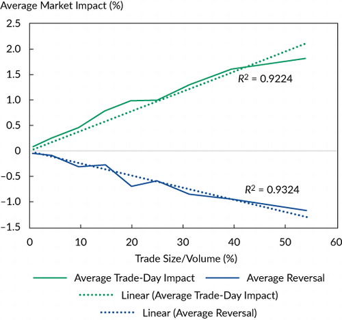
To demonstrate the linearity of the relationship between market impact and relative trade size, we grouped our unmodeled trade data into bins. We display in Figure 1 each bin’s average market impact and average trade size.¹³ (The subsequent reversal is also shown and will be discussed shortly.)

Figure 1. Average Market Impact by Trade Size

Source: Research Affiliates, based on data from Bloomberg.

Next, we formally identified the trade factor, the excess return that is linearly related to relative trade size, in the following regression:¹⁴$\begin{array}{c}{\text{Market impact}}_{i,t}=k_t\left(\frac{{\text{Dollar traded}}_i}{{\text{Dollar volume}}_i}\right)+{\epsilon }_i\\ =k_t\left({\text{Relative trade size}}_i\right)+{\epsilon }_i,\end{array}$ (2) where Dollar traded_i is the net dollar amount of security i traded by our set of indexes on the rebalancing day and Dollar volume_i is the total dollar trading volume for security i on that same rebalancing day.

The trade-day market impact factor, k₀ (where 0 denotes the trade day), was used to estimate the market impact for a trade of a given size on that day. The trade-day market impact represents the adverse return that the manager experiences when placing the trade. In other words, an abnormal return occurs on the underlying stock against the trade direction. The magnitude is expected to be the market impact factor k times relative trade size.¹⁵

We applied Equation 2$\begin{array}{c}{\text{Market impact}}_{i,t}=k_t\left(\frac{{\text{Dollar traded}}_i}{{\text{Dollar volume}}_i}\right)+{\epsilon }_i\\ =k_t\left({\text{Relative trade size}}_i\right)+{\epsilon }_i,\end{array}$ (2) using all the trades as a panel regression and present robust standard errors clustered on company and rebalance year (see Petersen 2009). Results are presented in Figure 2 and Table 3 together with, as robustness checks, separate results for the US market, the developed markets excluding the United States, and emerging markets, as well as for purchases only and sales only. Interestingly, we found no statistically significant evidence of a different impact for the three regions or of different trade directions for the same relative trade size.¹⁶, ¹⁷ Figure 2 also shows the reversal impact we measured by using the regression set forth in Equation 2$\begin{array}{c}{\text{Market impact}}_{i,t}=k_t\left(\frac{{\text{Dollar traded}}_i}{{\text{Dollar volume}}_i}\right)+{\epsilon }_i\\ =k_t\left({\text{Relative trade size}}_i\right)+{\epsilon }_i,\end{array}$ (2) , with cumulative market impact over four subsequent days after the trade as the dependent variable.¹⁸ The reversal impact factor, k₊₄, stands for the regression coefficient. The linearity of the reversal impact with respect to trade size is illustrated in Figure 1.

Figure 2. Market Impact and Reversal across Different Regions and Trade Directions

Note: Market impact factors are in percent, estimated by Equation 2.

Source: Research Affiliates, LLC, using data from Bloomberg.

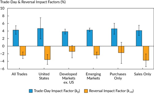
Table 3. Estimates and Significance of Trade-Day and Reversal Impact Factors

	All Trades	United States	Developed Ex. US	Emerging Markets	Purchases Only	Sales Only
Trade day
Impact factor (k0)	4.27%	4.70%	3.83%	4.30%	4.60%	4.16%
t-statistic	8.15	3.38	11.99	18.36	6.37	6.29
Reversal
Impact factor (k+4)	–2.42%	–3.53%	–1.42%	–2.34%	–1.74%	–3.73%
t-statistic	–5.67	–5.53	–1.74	–5.76	–1.25	–4.43

Note: Market impact factors are in percent, estimated by Equation 2.

Source: Research Affiliates, LLC, using data from Bloomberg.

We estimated the trade-day market impact factor for all trades as 4.27% and the reversal impact factor as –2.42%. Our results suggest that for every 10% of volume traded, the price of the underlying stock changed 43 bps, on average, against the trade on the trade day and that 24 bps of the change in price could be expected to be reversed in the subsequent four days.

The findings presented in Figure 2 are crucial because they imply the conjecture made by existing studies is not applicable to factor-investing strategies. Existing studies—for example, Petajisto (2011) and Chen et al. (2006)—analyzed the market impact costs of changes to popular benchmark indexes, such as the S&P 500 and the Russell 2000. Changes to these indexes are informative because they represent large and easily anticipated trades by the index funds. Chen et al. (2006) highlighted the adoption of “rarely used indexes” as one way that index investors can mitigate losses to arbitrageurs who attempt to front run the index changes. By their definition, factor-investing indexes, based on the low level of assets that track them relative to a traditional benchmark, are classified as “rarely used.” Our observations indicate, however, that market impact, in the absence of front running, can still be a significant cost to investors.

A hypothetical example will illustrate how the market impact occurs as a trading cost to investors: Say a trader executes a round-trip trade (buy, hold, and sell) of a stock with a market value of US$100 per share at a trade size equivalent to 10% of the stock’s daily trading volume. He observes a price level of US$100 and is able to buy the stock at an average price of US$100.43. After a few days, the value of the stock depreciates by 24 cents, on average, to US$100.19. At this point, the trader places a sell order on the stock and its price falls by 43 cents, on average. He sells at US$99.76. The trader’s total loss is 67 cents per share, on average (US$100.43 minus US$99.76), or 67 bps for the round trip. A few days after the sale, the price of the stock reverts 24 cents to US$100, producing no long-term impact on the stock price from the trading activity.

The index’s value is equivalent to the prices of the shares it holds. Under the influence of rebalancing, the index’s value and the returns to the index fund move in parallel. The implementation shortfall appears to be minimized, but fund investors still suffer an implicit market impact cost.

For simplicity, the hypothetical example shows the implicit cost of trading a single security. But to mitigate noise in estimations, we recommend using this cost model with aggregate trades rather than to forecast the cost of a single trade. In the next section, we demonstrate how to apply our model to baskets of trades induced by the rebalancing of broadly diversified indexes.

Application

The model for the market impact cost that we described is used in this section to estimate the costs associated with implementing a comprehensive list of factor-investing strategies, including value, income, low-beta (or low-volatility¹⁹), quality,²⁰ momentum, and multifactor funds. Some strategies can be characterized as core market indexes with style tilts; others appear to be satellite indexes that focus on a small subset of the entire universe. Using our index construction methodologies, we conducted backtests on strategies that are reasonably similar to commercially available funds. (Their security selection and weighting protocols are summarized in Appendix A.²¹) We simulated the resulting indexes’ performance by using data from Compustat and CRSP for US strategies and data from Worldscope and Datastream for international strategies.

We computed the expected market impact cost of all trades using Equation 2$\begin{array}{c}{\text{Market impact}}_{i,t}=k_t\left(\frac{{\text{Dollar traded}}_i}{{\text{Dollar volume}}_i}\right)+{\epsilon }_i\\ =k_t\left({\text{Relative trade size}}_i\right)+{\epsilon }_i,\end{array}$ (2) and our estimated market impact factor, $\overline{k}=0.03$.²² We then calculated the index-level market impact cost by aggregating the costs of all individual trades. The implicit cost of rebalancing a strategy equals the sum of the costs of all its underlying stocks’ trades, as follows:$\begin{array}{c}\text{Dollar cost of each trade}=E\left[{\text{Market impact}}_i\right]\Delta {\omega }_i\text{AUM}\\ =\overline{k}\left(\frac{{\text{Dollar traded}}_i}{{\text{Dollar volume}}_i}\right)\Delta {\omega }_i\text{AUM}\\ =\overline{k}\left[\frac{{\left(\Delta {\omega }_i\text{AUM}\right)}^2}{{\text{Dollar volume}}_i}\right];\end{array}$ (3) $\text{Dollar cost of strategy}={\displaystyle {\sum }_i\left[\overline{k}\frac{{\left(\Delta {\omega }_i\text{AUM}\right)}^2}{{\text{Dollar volume}}_i}\right]}.$ $\begin{array}{c}\text{Cost of strategy}=\frac{\text{Dollar cost}}{\text{AUM}}\\ =\overline{k}\left(\text{AUM}\right){\displaystyle {\sum }_i\left[\frac{{\left(\Delta {\omega }_i\right)}^2}{{\text{Dollar volume}}_i}\right]},\end{array}$ (4) where

$\overline{k}$ = estimated trade-day impact, $\overline{k}=0.03$

$\Delta {\omega }_i$ = change in weight to stock i for a given rebalancing of the strategy

Dollar volume_i = short-term median dollar volume observed on trade day for stock i Because we were estimating the expected cost of managing strategies without perfect foresight of trade-day volume of future rebalancing, dollar volume for Equations 3 and 4, as well as for the strategy characteristics throughout this “Application” section, is defined as the higher of 90-day median and 30-day median number of shares traded multiplied by the share price at current rebalancing.²³

This model can be applied for calculating both the cost and the capacity of the various strategies. For calculating cost, we assumed AUM equal to US$10 billion for US and developed-market strategies and AUM equal to US$1 billion for emerging-market strategies. To establish a uniform basis for comparing capacity, we set a fixed cost for all strategies at 50 bps a year and computed the corresponding AUM, effectively defining capacity as the largest amount of assets a strategy could hold without incurring more than 50 bps of market impact cost a year. The choice of 50 bps as the upper threshold is admittedly arbitrary, but we believe this approach is superior to estimating breakeven costs because excess returns are highly sensitive to the sample period.

The cost and capacity estimates of factor investing are more meaningful if one understands the drivers of high cost and of low capacity. For this purpose, we followed the approximation proposed by Aked and Moroz (2015) to attribute implementation costs to strategy characteristics:$\text{Cost of strategy}\approx \overline{k}\left(\text{AUM}\right)\varphi \frac{1}{\text{Portfolio volume}}\left(\text{Tilt}\right)\left(\text{Turnover}\right)\left(\text{Turnover concentration}\right),$ (5) where

$\text{Tilt}={\displaystyle {\sum }_i{\omega }_i\frac{{\omega }_i}{v_i}}$

$\text{Turnover}=\text{one-way turnover of the strategy =}\frac{{\displaystyle {\sum }_i\left|\Delta {\text{ω}}_i\right|}}{2}$

v_i = daily trading-volume weight of stock i

$\text{Turnover concentration }=\frac{2}{T_{Replace}+T_{Reweight}}\left[T_{Replace}+\frac{2}{2-T_{Replace}}\left(\Psi \right)\left(T_{Reweight}^2\right)\right]$

T_Replace = average turnover as a result of adding and removing securities

T_Reweight = average turnover as a result of reweighting existing securities

$\begin{array}{l}\Psi =\frac{E^{\omega }\left[{\delta }_i^2\right]}{{\left(E^{\omega }\left[\left|{\delta }_i\right|\right]\right)}^2}\\ E^{\omega }\left[x_i\right]=\frac{{\displaystyle {\sum }_{i\in Reweight}{\omega }_i{x}_i}}{{\displaystyle {\sum }_{i\in Reweight}{\omega }_i}}\\ {\delta }_i=\frac{\left|\Delta {\omega }_i\right|}{{\omega }_i}\end{array}$

$\varphi =\frac{1}{\text{Number of days over which the trade was executed}}$The strategy’s cost is inversely proportional to its portfolio volume, defined as the aggregate of median daily trade volume, in dollars, of all the stocks in the portfolio. This definition reflects the inverse relationship of cost to trading volume, as expressed in Equation 2$\begin{array}{c}{\text{Market impact}}_{i,t}=k_t\left(\frac{{\text{Dollar traded}}_i}{{\text{Dollar volume}}_i}\right)+{\epsilon }_i\\ =k_t\left({\text{Relative trade size}}_i\right)+{\epsilon }_i,\end{array}$ (2) . All else being equal, a small-cap portfolio would cost twice as much to implement as a large-cap portfolio if it had half the large-cap portfolio’s aggregate volume.

Tilt, in this context, is the degree to which the portfolio-holding weights deviated from a volume-weighted portfolio, which is the most liquid combination of a given set of stocks. (With respect to purchases made by the portfolio, if a trade’s expected cost was defined by Equation 2$\begin{array}{c}{\text{Market impact}}_{i,t}=k_t\left(\frac{{\text{Dollar traded}}_i}{{\text{Dollar volume}}_i}\right)+{\epsilon }_i\\ =k_t\left({\text{Relative trade size}}_i\right)+{\epsilon }_i,\end{array}$ (2) , then the lowest-cost combination would be to weight stocks by their daily volume.) The volume-weighted portfolio had a tilt of 1.0; holding all else equal, a portfolio with a tilt of 2.0 would experience twice as much market impact cost. Tilt and portfolio volume are complementary measures: Portfolio volume measures the liquidity of the selection of stocks, and tilt measures the liquidity of the weighting method applied to the selection. An investment strategy with a weighting methodology highly correlated with trading volume—for example, cap weighting—will tend to have a low cost.

A strategy’s annualized one-way turnover is another key determinant of cost; the strategy that requires the higher rate of trading is more costly to implement. Alone, however, one-way turnover is an inadequate indicator of cost. Consider two rebalancings with the same turnover rate. One requires buying US$100 million of the shares of a single large-cap company; the other requires buying US$10 million of the shares of each of 10 large-cap companies. Intuitively, we understand that the two portfolios would not incur the same costs: Highly concentrated trades are more costly to execute.

The turnover concentration metric captures the degree to which costs are reduced by spreading trades across the portfolio. Factor strategies that invest in small subsets of the market—momentum is a good example—tend to have high turnover concentration because they routinely require that the manager completely eliminate a few existing positions and buy into new positions. In contrast, broad market indexes that reweight constituents back to predetermined and stable weights tend to have low turnover concentration. Additionally, strategies that rebalance frequently, such as quarterly versus annually, will tend to have lower turnover concentration.

The number of days over which a single trade is executed also affects cost. (Ratcliffe et al. 2017 also discussed this point.) Consider two trades of the same amount. One requires buying US$100 million of a large-cap company today; the other buys US$50 million today and buys another US$50 million at a later date. Assuming the volume is the same for both trading days, the cost of the trade would be reduced by one-half, according to Equation 2$\begin{array}{c}{\text{Market impact}}_{i,t}=k_t\left(\frac{{\text{Dollar traded}}_i}{{\text{Dollar volume}}_i}\right)+{\epsilon }_i\\ =k_t\left({\text{Relative trade size}}_i\right)+{\epsilon }_i,\end{array}$ (2) . More formally, cost can be reduced by N times if all of the trades for one rebalancing are executed over N distinct periods ($\varphi =1/N$ in Equation 5$\text{Cost of strategy}\approx \overline{k}\left(\text{AUM}\right)\varphi \frac{1}{\text{Portfolio volume}}\left(\text{Tilt}\right)\left(\text{Turnover}\right)\left(\text{Turnover concentration}\right),$ (5) ), which was set to 1.0 for our study. But an index implementer who is less concerned with tracking error might choose to spread trades over several days, which should reduce implementation costs. Note that this discussion describes the execution of a strategy rather than a characteristic and is different from rebalancing frequency (e.g., annually versus quarterly).

Table 4 displays the expected costs, as defined in Equation 4$\begin{array}{c}\text{Cost of strategy}=\frac{\text{Dollar cost}}{\text{AUM}}\\ =\overline{k}\left(\text{AUM}\right){\displaystyle {\sum }_i\left[\frac{{\left(\Delta {\omega }_i\right)}^2}{{\text{Dollar volume}}_i}\right]},\end{array}$ (4) , and capacities at a hypothetical cost of 50 bps a year of an array of popular US factor-investing indexes together with their simulated performance from 1968 through 2016.²⁴ The table also shows strategy characteristics that are helpful in explaining differences in implementation costs. We are limiting the following discussion to US strategies, but we present similar results for international developed and emerging markets in the online supplemental material (available at www.tandfonline.com/doi/suppl/10.1080/0015198X.2019.1567190).

Table 4. Market Impact Costs and Liquidity Characteristics of US Factor-Investing Strategies, 1968–2016

Strategy	Return	Volatility	Market Impact Cost	Capacity (US$ billions)	Portfolio Volume (US$ millions)	Turnover	Turnover Concentration	Tilt
Value strategies
Concentrated value	11.6%	16.1%	0.28%	17.7	39,299	25.1%	77.2%	1.5
Fundamental indexing	11.6	14.8	0.02	290.7	96,651	11.4	21.9	1.6
Income strategies
High dividend	12.1%	14.4%	0.61%	8.2	13,464	20.1%	67.5%	9.3
Dividend growth	12.1	14.1	0.76	6.6	26,016	37.5	49.5	4.5
Low-volatility strategies
Minimum volatility	11.2%	13.3%	0.39%	12.9	34,290	24.8%	73.3%	2.3
Low volatility	11.1	12.0	1.90	2.6	21,382	71.6	84.3	2.1
Defensive	10.6	13.2	0.07	72.7	68,539	14.1	83.6	1.5
Fundamental low volatility	12.5	13.4	0.05	107.8	42,257	23.1	44.9	1.5
Quality strategies
Quality	11.1%	15.7%	0.37%	13.5	35,029	23.8%	71.9%	1.3
Conservative profitable	11.5	14.2	0.11	44.6	35,794	19.1	38.4	1.5
Momentum strategies
Sharpe momentum	11.9%	17.3%	2.05%	2.4	35,797	108.5%	88.4%	1.3
Standard momentum	11.9	17.7	2.72	1.8	37,928	155.8	90.2	1.3
Multifactor strategies
Quality/value/low volatility	11.2%	14.1%	0.22%	22.6	52,410	23.4%	71.2%	1.6
Mathematical beta 6	11.5	14.9	0.12	40.6	99,997	36.8	47.9	2.3
Dynamic multifactor	12.6	14.8	0.23	21.3	96,739	51.6	60.0	1.8
Other
Equal weight	10.8%	17.1%	0.20%	25.0	109,263	29.8%	47.6%	2.0

Notes: Return, volatility, and turnover are averaged over the period. Other characteristics are based on the most recent rebalancing up to the end of 2016. Market impact costs assume US$10 billion in AUM and are averaged over the most recent five years, with the cost of each trade capped at 2%. (Note that this assumption would imply a trade that consumes 66% of daily volume. Many practitioners would be unwilling to trade more than this percentage or would stop trading upon incurring a cost of 2%. This limit also reduced the incidence of volume data outliers.) Capacity is the estimated AUM at which the strategy is expected to have 50 bps of market impact cost. See Appendix A for strategy descriptions.

Source: Research Affiliates, based on data from Worldscope and Datastream.

The two momentum strategies stand out as the most expensive to implement. At US$10 billion in AUM, the Sharpe momentum and standard momentum strategies are estimated to incur annual market impact costs of, respectively, 2.05% and 2.72%, more than offsetting their simulated excess return. At 50 bps of annual cost, they can manage only, respectively, US$2.4 billion and US$1.8 billion in total assets. The momentum strategies have high turnover rates, high turnover concentrations, and low portfolio volumes relative to strategies of other styles. Collectively, these characteristics imply they have concentrated or illiquid holdings, completely trade out of and into a few positions, and do so at a fast pace. All of these traits contribute to their high cost of implementation.²⁵ In contrast, they have the lowest tilt, at 1.3, which suggests their weighting by market capitalization (or a variant) mitigates some of the trading challenges.

Income strategies also incur noticeably high costs. At the assumed level of US$10 billion in assets, the high-dividend and dividend growth strategies have annual costs of, respectively, 61 bps and 76 bps. Their turnover rates are much lower than the momentum strategies because they both use stringent banding rules. The main causes of their high costs are their low portfolio volumes and high tilts, which are probably the result of investing in a small number of the highest-yielding companies and weighting their positions by yield. Investors who seek steady streams of healthy dividends pay a hidden price in the form of market impact costs.

At the other extreme, fundamental indexing is the least expensive to implement. At US$10 billion in AUM, it has the lowest annual market impact cost (2 bps) and, at the annual cost ceiling of 50 bps, the highest capacity (US$291 billion). Fundamental indexing is a broad market indexing strategy, as evidenced by its high portfolio volume of US$97 billion. Distributed over four quarters, its turnover primarily consists of restoring existing constituents to their fundamental weights; accordingly, both its turnover rate and turnover concentration are the lowest among the factor-investing strategies in our sample. The tilt of fundamental indexing is also low (on a par with cap-weighted strategies), indicating that fundamental size is highly correlated with trading volume. In contrast, the concentrated value strategy has significantly lower capacity. A strong bet on a target factor may have high expected return, but the trade-off is higher implementation cost and more risk.

The low-volatility (or low-beta) group offers the most interesting observations. Although the strategies in this category have distinctive methodologies and characteristics, they all achieve their primary investment objective—respectable returns with low risk. They have strikingly different costs, however, ranging from 1.9% for the low-volatility strategy (almost as high as momentum) to only 5 bps for the fundamental low-volatility strategy and 7 bps for the defensive strategy (almost as low as fundamental indexing).

The extended high–low range underlines the importance of index design. The low-volatility strategy has the simplest methodology: Select the 20% of stocks with the lowest volatility and weight them by the inverse of volatility. Empirically, these straightforward selection and weighting rules have the further merit of producing the lowest simulated volatility. Nevertheless, a 185 bp difference in expected implementation costs is too great to overlook.

The multifactor strategies, which can be viewed as mixtures of single-factor portfolios, have moderate costs despite their added complexity. Their capacities are well above those of the minimum-volatility and quality strategies, which constitute two-thirds of the quality/value/low-volatility strategy. Mixing multiple single-factor portfolios tends to lower costs because the constituent strategies find liquidity in different subsets of the market. (Witness the multifactor strategies’ high portfolio volumes, ranging from US$52.410 billion to US$99.997 billion.) Interestingly, the mathematical beta 6 and dynamic multifactor strategies do not have higher costs, despite their investments in momentum stocks. Mixing factors diversifies the holdings and reduces turnover concentration. Recall that the two momentum strategies in our analysis had portfolio volumes of US$35.8 billion and US$37.9 billion and turnover concentrations of 88.4% and 90.2%, respectively. With multiple factor exposures that include momentum, the portfolio volume measures jump to US$96.739 billion (for the dynamic multifactor strategy) and US$99.997 billion (for the mathematical beta 6 strategy)—as high as the portfolio volume of the fundamental indexing strategy—and turnover concentration drops to the 48%–60% level.

Understanding implementation costs in relation to strategy characteristics may allow providers to offer, and investors to select, factor-investing funds with better long-term net-of-cost returns than was previously possible. Given a strategy’s specific investment objective, some undesirable characteristics are admittedly unavoidable. For example, momentum strategies inherently come with high turnover rates, and dividend-yield strategies entail high concentrations. Still, refined design techniques—such as spreading rebalances over multiple distinct periods, constraining stock selection rules to limit turnover, and weighting selections by a metric correlated with a stock’s trading volume—should be considered whenever possible.²⁶

Limitations of Our Research

All models are imperfect, and ours has at least two weaknesses. First, our market impact model potentially overestimates the cost of large changes in positions because we assumed all portfolio managers rebalance a given indexing strategy on the same trade day. Experienced managers who care about trading costs are unlikely to place orders on an exchange consisting of multiple orders of the underlying security’s average daily volume. Moreover, our model undoubtedly misestimates the cost of large trades that the market anticipates, such as S&P 500 reconstitutions. In these cases, arbitrageurs may step up to provide liquidity around the trade day (see, e.g., Petajisto 2011). To the extent that large trades are predictable, the market impact relative to trade size should be recalibrated.

Second, a related and possibly more important limitation is that users of our model cannot precisely estimate relative trade sizes in advance of rebalancing a particular strategy. Other investment strategies of similar or opposite style might rebalance on the same day, competing for liquidity from, or providing liquidity to, one another. In addition, sophisticated managers may turn to off-exchange facilities, such as crossing networks or dark pools.

For these reasons, we provide our framework, results, and discussion merely to illuminate the less obvious challenges involved in designing and selecting factor-investing strategies. The model enables market participants to gauge the relative implementation costs of various strategies and to compare their capacities on a fair basis. We contend that the model captures salient factors, but we do not claim it definitively quantifies or accurately predicts actual market impact costs.

Conclusion

Assets have been flowing steadily from actively managed funds to factor-investing strategies since about 2008. The significant growth in factor investing leads to potential capital erosion when trading volume affects security prices: Investors do not get the price they see but the price they pay. Transaction costs, including implicit market impact costs, are a key element in determining the returns that investors actually earn. An index fund’s NAV moving in parallel with the index return creates the illusion that the portfolio has no market impact cost. Nonetheless, the cost is reflected implicitly in both the index and the tracking funds, whose values change simultaneously with the prices of their holdings. The returns of both are lower than they would have been in the absence of trading.

Our analysis uncovered the implicit cost of market impact by studying the rebalancing information of a suite of live factor-investing indexes. We found significant evidence of market impact on the rebalancing day and a subsequent price reversal over the next four days. We found that the magnitude of the price impact is predictable because it is directly related to the security’s liquidity and the size of the trade. Specifically, we identified that a fund incurs approximately 30 bps of trading costs as a result of market impact for every 10% of a stock’s ADV traded in aggregate by the funds tracking a factor-investing index.

Extending our observations to a cost model, we analyzed the trading costs of the most common and popular factor-investing strategies. In contrast to traditional benchmarks, these strategies use various stock selection and weighting methods to target exposures to similar (or the same) factors, resulting in dramatically different liquidity profiles and trading patterns among the indexes. Knowing what drives costs is perhaps more important than the cost estimations themselves. Therefore, we presented a cost attribution framework to contrast the characteristics of strategies and relate them to the specific cost estimates.

We found that strategies with low portfolio volumes, high turnover rates, high concentration of turnover, and strong tilts away from volume-weighted benchmarks tend to experience high trading costs. This finding is helpful for investors evaluating the feasibility of investment objectives and for index providers in making sensible design decisions. Momentum strategies are generally costly because they require a high rate of turnover and a high concentration of turnover. Income strategies are also generally costly because they hold concentrated sets of, and tilt weights toward, the highest-yielding stocks. In other types of factor investing, we showed that strategies that offer similar factor exposures, such as value and low-beta strategies, can have vastly different expected costs. Our cost attribution framework sheds light on how practitioners can make an appropriate trade-off between expected net-of-cost return and strategy characteristics.

Our research enhances the market microstructure literature by demonstrating the market impact made collectively by indexers, even for strategies that have not attracted nearly as many assets as traditional benchmarks. In addition, our research makes a significant advance in understanding the costs and capacities of factor investing. Previous studies identified capacities of certain factor-investing methods. Our simple model of market impact costs and standardized comparisons of cost-sensitive strategy characteristics can be easily and broadly applied to all systematic strategies that can be backtested. Our work not only includes cost estimations for a broad set of strategies across factors, styles, and regions, but it also explains how strategies with certain characteristics will reach capacity sooner than others.

Acknowledgments

We would like to thank the editors and the reviewers for their very constructive feedback. We are grateful to Mike Aked, Rob Arnott, Chris Brightman, Jaynee Dudley, Cam Harvey, Kay Jaitly, Vitali Kalesnik, Shane Shepherd, and Katy Sherrerd for the discussions and assistance.

Notes

¹ Some academic journal articles use the term “factor investing” broadly to include strategies that buy one portfolio of companies and short another portfolio of companies with distinctively different characteristics. We refer to factor investing, however, as commercially available long-only alternative indexing with transparent rules for security selection and weighting. These strategies that systematically target exposure to alternative factors beyond the market are often referred to as “smart beta” strategies.

² Factor investing has other risks. Specifically, overfitting or data mining in historical backtests may lead investment managers to overestimate the future prospects of factor-investing strategies that have only short track records—or none at all (Harvey, Liu, and Zhu 2016). Our study mitigates part of the data-mining risk by quantifying realizable returns net of market impact costs.

³ For example, the MSCI USA Quality Index, MSCI USA Momentum Index, and S&P 500 Low Volatility Index cover only about 20% of their parent indexes, and their reported turnover rates are, respectively, 20%, 96%, and 53% (MSCI 2017a, 2017b; PowerShares 2017).

⁴ The indexes are described at www.ftse.com/products/indices/rafi.

⁵ The literature on cost and investment capacity is large and diverse, and our review of past contributions is limited. For a more comprehensive review, see O’Neill and Warren (2016) for an excellent survey of many more articles related to all aspects of investment capacity.

⁶ Additionally, assuming that cost is directly proportional to turnover is perhaps too simple. Trading the same amount of a mega-cap company versus a micro-cap company will certainly result in different costs.

⁷ For instance, low-beta (or low-volatility) strategies can have different alphas depending on which factor model is used.

⁸ We also looked at the market behavior before the rebalancing date for indications of front running. We found some evidence of front running on the day before the rebalancing (buys with positive and sells with negative market impacts on the day before the trade), but it was statistically insignificant and on a small scale relative to the impact registered on the actual rebalancing date.

⁹ We excluded 1,131 outlying observations (≃2.2% of our sample) to arrive at this final dataset. Specifically, we excluded all observations in which the dollars traded were greater than two-thirds of the volume on the trade date, because the stated assumption of all trading occurring on the rebalancing day probably failed for these trades. Additionally, we excluded those observations with large abnormal returns (±15%) on the rebalancing day or any of the four subsequent days because these returns were probably related to company-specific events beyond the rebalancing of indexes and only added noise to our analyses.

¹⁰ Prior studies on the costs of front-running activities to investors of passive indexing, such as Petajisto (2011) and Chen et al. (2006), described indexes’ demand for liquidity with the level of indexing. This measure is helpful for estimating aggregate costs to all investors of a traditional passive benchmark that incurs turnover primarily when stocks are added to or deleted from the composition. Because factor-investing strategies require many more trades beyond additions to and deletions from compositions, however, the relative trade size of the component securities is the more relevant characteristic of our subject.

¹¹ Sensitivities to regional and industry markets for each stock (β_i,Regional, β_i,Industry) were estimated with 1.5 years of daily returns centered on the trade day. We found that estimation periods other than 1.5 years made no material difference to our analyses.

¹² We also experimented with controlling for other common equity factors—namely, size, value, and momentum—and found they generally did not enhance the regression fit.

¹³ Barclay and Warner (1993) hypothesized that informed traders who break trades into certain sizes that are neither too big nor too small are the primary causes of stock price movement, which implies that market impact will have a concave relationship to relative trade size. We observed no empirical evidence to support or reject this “stealth-trading” hypothesis. We prefer the linear approach for its simplicity.

¹⁴ Relative trade size as a key determinant has been adopted by a few other authors in microstructure literature—for example, Chiyachantana et al. (2004). We also expanded Equation 2$\begin{array}{c}{\text{Market impact}}_{i,t}=k_t\left(\frac{{\text{Dollar traded}}_i}{{\text{Dollar volume}}_i}\right)+{\epsilon }_i\\ =k_t\left({\text{Relative trade size}}_i\right)+{\epsilon }_i,\end{array}$ (2) to include other control variables commonly thought to be related to trading costs (market cap, return volatility, and return momentum at various horizons). We found, however, that the market impact cost depends primarily on relative trade size. Because the inclusion of other variables did not statistically or economically change the results, we do not report those findings here.

¹⁵ We forced the intercept through zero for clearer interpretation: No trading = No impact.

¹⁶ This finding is in conflict with Domowitz, Glen, and Madhavan (2001) and Chiyachantana et al. (2004), who reported the market impact cost to be higher in the emerging markets after they controlled for such determinants as market cap and return volatility. A potential explanation is that since the early 2000s, the emerging markets no longer warrant higher market impact costs because they have become more liberal and have established stronger shareholder protections.

¹⁷ The implicit cost of selling is on a par with buying. Our analyses do not fully represent the cost of short selling, which requires an additional cost of borrowing shares.

¹⁸ We also looked for evidence of reversal up to 20 days after the trade. We found, however, that the reversal effect is concentrated in the first four days following a trade. Note that we observed slightly stronger and significantly faster price reversal than Petajisto (2011), who studied constituent changes to the S&P 500 and the Russell 2000 from 1990 to 2005.

¹⁹ The low-beta anomaly advanced by Frazzini and Pedersen (2014) is the relevant factor, but we extended our analysis to cover the broader low-volatility anomaly that included popular strategies with relatively long records, such as minimum volatility.

²⁰ Definition of quality varies across practitioners. For this study, we broadly included strategies that exploit anomalies related to companies’ profitability, leverage, earnings variability, and growth.

²¹ To allow for apples-to-apples comparisons, we modified the methodologies slightly to have consistent starting universes, regional definitions, and rebalancing dates. We included South Korea in emerging markets despite conflicting classifications by popular index providers. All annual rebalances occurred at the end of June; semiannual rebalances at the end of June and December; and quarterly rebalances at the end of March, June, September, and December.

²² We estimated the cost of two-way turnover to be 6.7 bps for each 1% of volume traded, and we rounded the impact factor of a one-way trade to 3 bps (0.03%). Readers who are interested in estimating the implementation cost of a factor-investing strategy that assumes a different impact level can simply scale the cost estimates we present in Table 4.

²³ The 90-day horizon captured a robust estimate of the median number of shares traded, and the 30-day horizon captured a sudden spike (if any) in number of shares traded; the current share price was the best estimate of share price at the upcoming rebalancing.

²⁴ The costs were estimated with five years of rebalancing, and the market volume was estimated through the end of 2016. In reality, the expected costs are time varying; estimations across all strategies, as indicated by Equation 3$\begin{array}{c}\text{Dollar cost of each trade}=E\left[{\text{Market impact}}_i\right]\Delta {\omega }_i\text{AUM}\\ =\overline{k}\left(\frac{{\text{Dollar traded}}_i}{{\text{Dollar volume}}_i}\right)\Delta {\omega }_i\text{AUM}\\ =\overline{k}\left[\frac{{\left(\Delta {\omega }_i\text{AUM}\right)}^2}{{\text{Dollar volume}}_i}\right];\end{array}$ (3) , would be higher during times when liquidity was systematically low; see Huberman and Halka (2001).

²⁵ Practitioners such as Beck, Hsu, Kalesnik, and Kostka (2016) have argued against using momentum as a stand-alone factor-investing strategy.

²⁶ The first and second techniques, staggered rebalancing and applying asymmetrical rules for establishing or maintaining positions, were also proposed by Novy-Marx and Velikov (2016).

Appendix A.

Strategy Simulation Methodologies

Table

Strategy	Description
1. Concentrated value	The semiannually rebalanced strategy selected the top 20% from the large-cap and midcap universe on the basis of a value score calculated from the ratios of price to book value, price to earnings, and enterprise value to cash flow from operations. It weighted selections by market cap times the value score.
2. Fundamental indexing	The strategy selected and weighted companies according to four fundamental measures of company size: book value, cash flow, dividends plus buyback, and adjusted sales. It was implemented in four annually rebalanced tranches in such a way that trades were spread over four quarters.
3. High dividend	After screening for dividend growth and dividend coverage, the annually rebalanced strategy selected 100 stocks by dividend yield from the large-, mid-, and small-cap universes and weighted selections by indicated dividend yield.
4. Dividend growth	For US market simulations, the strategy rebalanced quarterly, selecting companies from the top 1,500 by market cap that had stable or increasing dividends in the last 20 years. For developed-market simulations, stocks with stable or increasing dividends in the last 10 years were selected from the large-, mid-, and small-cap universes and weighted by indicated dividend yield. In emerging-market simulations, stock selections were based on growing earnings and high dividend yields and were weighted by annual dividend yield. Portfolios for both developed and emerging markets were rebalanced semiannually.
5. Minimum volatility	The strategy minimized the volatility of a large- and midcap portfolio by means of a constrained optimization. Constraints included maximum single-holding weight, country and sector active weights, and turnover limits. The optimization was recomputed semiannually.
6. Low volatility	The quarterly rebalanced strategy selected the 20% lowest-volatility stocks from the parent universe and weighted them by 1/Volatility.
7. Defensive	The strategy reweighted stocks from the parent universe according to a stability score, which captured low volatility, low earnings variability, low leverage, and high return on assets. The portfolio was rebalanced annually.
8. Fundamental low volatility	The strategy selected companies from each sector and region of the parent universe with low valuations and low systemic risk and weighted selections by their fundamental size. It was implemented in four annual rebalancing tranches in such a way that trades were spread over four quarters.
9. Quality	The semiannually rebalanced strategy selected companies from the large- and midcap parent universe on the basis of a quality score that combined high return on equity, low debt to equity, and low earnings variability. Selections were weighted by market cap times a quality score.
10. Conservative profitable	The strategy selected the top 25% of large companies with high profitability and low investment and weighted selections by fundamental size. It was implemented in four annual rebalancing tranches in such a way that trades were spread over four quarters.
11. Sharpe momentum	The strategy selected companies from the large- and midcap parent universe on the basis of a momentum score reflecting prior 6-month and 12-month Sharpe ratios. Selections were weighted by market cap times a momentum score. The portfolio was rebalanced semiannually, with additional ad hoc rebalances triggered by volatility spikes.
12. Standard momentum	The quarterly rebalanced strategy selected the top third of companies from the large-cap and midcap parent universe by momentum, defined as prior-year return. It skipped the most recent month and weighted selections by market cap.
13. Mathematical beta 6	The quarterly rebalanced strategy equally weighted six factor indexes: value, momentum, midcap, low volatility, profitability, and investment. Each factor was constructed by selecting half the companies from regional large-cap universes by characteristics, and the selections were weighted via five diversification methods.
14. Quality/value/low volatility	The fund equally weighted quality, low-volatility, and value strategies that reweighted the large-cap and midcap parent universe by fundamental size.
15. Dynamic multifactor	At every quarter, the strategy dynamically weighted five factor indexes—value, low volatility, quality, momentum, and size—based on long-term reversal and short-term momentum. The large-cap size factor was constructed by selecting the top 25% of the large-cap and midcap company universes (50% for momentum). Selections were then weighted by fundamental size (market capitalization for momentum). The small-cap size factor was constructed by equally weighting the other four factors constructed within the small-company universe.
16. Equal weight	The quarterly rebalanced strategy equally weighted all stocks in the parent universe.

References

- Aked, Michael, and Max Moroz. 2015. “The Market Impact of Passive Trading.” Journal of Trading, vol. 10, no. 3: 5–12.
- Almgren, Robert, and Neil Chriss. 2001. “Optimal Execution of Portfolio Transactions.” Journal of Risk, vol. 3, no. 2: 5–39.
- Almgren, Robert, Chee Thum, Emmanuel Hauptmann, and Hong Li. 2005. “Direct Estimation of Equity Market Impact.” Risk, vol. 18, no. 7: 58–62.
- Barclay, Michael, and Jerold Warner. 1993. “Stealth Trading and Volatility: Which Trades Move Prices?” Journal of Financial Economics, vol. 34, no. 3: 281–305.
- Beck, Noah, Jason Hsu, Vitali Kalesnik, and Helge Kostka. 2016. “Will Your Factor Deliver? An Examination of Factor Robustness and Implementation Costs.” Financial Analysts Journal, vol. 72, no. 5: 58–82.
- Berk, Jonathan, and Richard Green. 2004. “Mutual Fund Flows and Performance in Rational Markets.” Journal of Political Economy, vol. 112, no. 6: 1269–95.
- Berkowitz, Stephen, Dennis Logue, and Eugene Noser. 1988. “The Total Cost of Transactions on the NYSE.” Journal of Finance, vol. 43, no. 1: 97–112.
- Bertsimas, Dimitris, and Andrew Lo. 1998. “Optimal Control of Execution Costs.” Journal of Financial Markets, vol. 1, no. 1: 1–50.
- Chen, Honghui, Gregory Noronha, and Vijay Singal. 2006. “Index Changes and Losses to Index Fund Investors.” Financial Analysts Journal, vol. 62, no. 4: 31–47.
- Chen, Zhiwu, Werner Stanzl, and Masahiro Watanabe. 2002. “Price Impact Costs and the Limit of Arbitrage.” EFA 2002 Berlin Meetings Presented Paper (26 February); Yale ICF Working Paper No. 00-66.
- Chiyachantana, Chiraphol, Pankaj Jain, Christine Jiang, and Robert Wood. 2004. “International Evidence on Institutional Trading Behavior and Price Impact.” Journal of Finance, vol. 59, no. 2: 869–98.
- Domowitz, Ian, Jack Glen, and Ananth Madhavan. 2001. “Liquidity, Volatility and Equity Trading Costs across Countries and over Time.” International Finance, vol. 4, no. 2: 221–55.
- Frazzini, Andrea, Ronen Israel, and Tobias Moskowitz. 2012. “Trading Costs of Asset Pricing Anomalies.” Fama-Miller Working Paper, Chicago Booth Research Paper No. 14-05 (5 December).
- Frazzini, Andrea, and Lasse Pedersen. 2014. “Betting against Beta.” Journal of Financial Economics, vol. 111, no. 1: 1–25.
- Gabaix, Xavier, Parameswaran Gopikrishnan, Vasiliki Plerou, and H. Eugene Stanley. 2006. “Institutional Investors and Stock Market Volatility.” Quarterly Journal of Economics, vol. 121, no. 2: 461–504.
- Harvey, Campbell, Yan Liu, and Heqing Zhu. 2016. “… and the Cross-Section of Expected Returns.” Review of Financial Studies, vol. 29, no. 1: 5–68.
- Huberman, Gur, and Dominika Halka. 2001. “Systematic Liquidity.” Journal of Financial Research, vol. 24, no. 2: 161–78.
- Huberman, Gur, and Werner Stanzl. 2005. “Optimal Liquidity Trading.” Review of Finance, vol. 9, no. 2: 165–200.
- Investors Mutual Limited2012. “Analysis of Institutional Fund Capacity: Implications for Investment and Execution.” White paper.
- Jones, Charles, and Marc Lipson. 2001. “Sixteenths: Direct Evidence on Institutional Execution Costs.” Journal of Financial Economics, vol. 59, no. 2: 253–78.
- Kahn, Ronald, and Michael Lemmon. 2016. “The Asset Manager’s Dilemma: How Smart Beta Is Disrupting the Investment Management Industry.” Financial Analysts Journal, vol. 72, no. 1: 15–20.
- Kahn, Ronald, and Scott Shaffer. 2005. “The Surprisingly Small Impact of Asset Growth on Expected Alpha.” Journal of Portfolio Management, vol. 32, no. 1: 49–60.
- Keim, Donald, and Ananth Madhavan. 1997. “Transactions Costs and Investment Style: An Inter-Exchange Analysis of Institutional Equity Trades.” Journal of Financial Economics, vol. 46, no. 3: 265–92.
- Mayston, D.. 2012. “Global T-Cost Model: Specification.” Trading research, BlackRock.
- MSCI2017a. “MSCI USA Quality Index (USD) Factsheet.”28 (April) .
- MSCI2017b. “MSCI USA Momentum Index (USD) Factsheet.”28 (April) .
- Novy-Marx, Robert, and Mihail Velikov. 2016. “A Taxonomy of Anomalies and Their Trading Costs.” Review of Financial Studies, vol. 29, no. 1: 104–47.
- O’Neill, Michael, and Geoffrey Warren. 2016. “Evaluating Fund Capacity: Issues and Methods.” CIFR Paper No. 124/201627 (September) .
- Perold, Andre. 1988. “The Implementation Shortfall: Paper versus Reality.” Journal of Portfolio Management, vol. 14, no. 3: 4–9.
- Petajisto, Antti. 2011. “The Index Premium and Its Hidden Cost for Index Funds.” Journal of Empirical Finance, vol. 18, no. 2: 271–88.
- Petersen, Mitchell. 2009. “Estimating Standard Errors in Finance Panel Data Sets: Comparing Approaches.” Review of Financial Studies, vol. 22, no. 1: 435–80.
- PowerShares2017. “PowerShares S&P 500® Low Volatility Portfolio Prospectus.”24 (February) .
- Ratcliffe, Ronald, Paolo Miranda, and Andrew Ang. 2017. “Capacity of Smart Beta Strategies from a Transaction Cost Perspective.” Journal of Index Investing, vol. 8, no. 3: 39–50.
- S&P Dow Jones2013. “10 Years Later: Where in the World Is Equal Weight Indexing Now?”22 (April) .
- Scobie, David. 2013. “Keep Your Eyes on the Size: Fund Manager Capacity and Why It Matters.” White paper (March) .
- Shirbini, Eric. 2015. “Implementation of Multi-Smart Factor Indices.” Presentation to CFA Society Netherlands12 (March) www.cfasociety.org/netherlands/Documents/ Slides_CFA_Implementation_of_Multi_Smart_Factor_Indices.pdf .
- Vangelisti, Marco. 2006. “The Capacity of an Equity Strategy.” Journal of Portfolio Management, vol. 32, no. 2: 44–50.