The Revenge of the Stock Pickers

Abstract

When an exchange-traded fund (ETF) trades heavily around a theme, correlations among its constituents increase significantly. Even some securities that have little or negative exposure to the theme itself begin to trade in lockstep with other ETF constituents. In other words, because ETF investors are agnostic to security-level information, they often “throw the baby out with the bathwater.” As the prices of individual stocks get dragged up or down with ETFs, these mispricings can become significant, and the profits realized by taking advantage of them may present an opportunity for stock pickers.

Disclosure: The authors work for an active investment manager involved in stock picking. The views expressed in this article are those of the authors and do not necessarily reflect the views of T. Rowe Price. Further information can be found at the end of this paper.

Editor’s note

Submitted 10 September 2018

Accepted 7 January 2019 by Stephen J. Brown

The views expressed are those of the authors, are subject to change without notice, and may differ from those of other T. Rowe Price associates. Information and opinions are derived from proprietary and nonproprietary sources deemed to be reliable; the accuracy of those sources is not guaranteed. This material does not constitute a distribution, offer, invitation, recommendation, or solicitation to sell or buy any securities; it does not constitute investment advice and should not be relied upon as such. Investors should seek independent legal and financial advice, including advice as to tax consequences, before making any investment decision. Past performance is not a reliable indicator of future performance. All investments involve risk. The charts and tables are shown for illustrative purposes only.

Exchange-traded funds (ETFs) now account for 30% of all trading volume on US exchanges, up from less than 2% in 2000.¹ This trend may have created opportunities for stock pickers. When an ETF trades heavily around a theme, correlations among its constituents increase significantly. Even some securities that have little or negative exposure to the theme itself begin to trade in lockstep with other ETF constituents. In other words, because ETF investors are blind to security-level information, they often “throw the baby out with the bathwater.” As the prices of individual stocks get dragged up or down with ETFs, these mispricings can become significant, and the profits realized by taking advantage of them may represent one of the hidden costs to ETF investing. In a recent editorial, Giamouridis (2017) called for more research on this topic. He referred to “higher trade commonality in ETF constituent stocks (in down markets), increased commonality in their liquidity/market impact, and less idiosyncratic risk compared with nonconstituent stocks” (11). And he emphasized that future research should clarify how volatility and correlations change as well as the likelihood of price deviations from fundamentals (and reversions).

To answer this call for research and, importantly, to estimate the size of this opportunity for stock pickers, we designed a simple, contrarian trading strategy that buys oversold constituents when an ETF sells off in a high-volume panic. We focused on the downside because research has shown that investors are less rational when faced with losses than when faced with gains. Page and Panariello (2018), for example, showed that extreme downside correlations are almost always higher than upside correlations. They argued that “in financial markets, fear is more contagious than optimism” (27).

We identified oversold constituents by their beta to the ETF. We used nine sector ETFs because they are more susceptible to speculative, retail-oriented trading than broad index ETFs. We also used an S&P 500 ETF and a small-cap ETF. Giamouridis (2017, 11) specifically called for research to cover “not only stocks in broad market indexes that are ETF constituents but also specific segments of the equity market,” such as sectors.

We don’t suggest that anyone implement this strategy without fundamental oversight, but our results were striking: When high-volume selloffs occur, ETF investors may be leaving as much as 200–300 bps of alpha on the table for stock pickers to capture over the following 40 days. Across ETFs, such events occurred, on average, 30 times per year, for a total of 240 events throughout our study period (4 January 2010–29 December 2017).

This strategy doesn’t require any stock-picking skills other than the ability to measure a stock’s beta to its ETF. We suspect stock pickers can capture even more alpha from ETF investors. They can carefully analyze why the ETF is selling off and whether certain constituents are simply being dragged down with it for no good fundamental reason. Here, our goal is merely to estimate the size of the opportunity, because it’s impossible to backtest a discretionary, fundamental approach.

Prior Research on Constituent Blindness and the Impact of Index Investing

Cahan, Bai, and Yang (2018) suggested that most ETF investors don’t focus on the fundamentals of the underlying constituents.² They referred to the “arbitrage opportunity” that arises when “the short-term trading activity in an ETF is inconsistent with the real-world fundamentals of the underlying stocks” (1). They used the term “arbitrage” in an informal way, not in the academic sense of riskless profit. But they showed that investors can generate alpha if they select ETFs based on the fundamentals of the constituents. Cahan et al. found that sector ETFs are the most disconnected from fundamentals, but the effect is also present for broad market and smart beta ETFs. Although we reach similar conclusions, our approach is different in that we picked stocks (i.e., we looked for mispricings within ETF constituents) whereas Cahan et al. picked ETFs (they looked for mispricing across ETFs, based on stock-level analysis).

Similarly, Wurgler (2010) and others have documented evidence of the effects of indexing on security-level co-movements. When a stock is added to an index, its correlation with its peer index constituents immediately increases (see, e.g., Barberis, Shleifer, and Wurgler 2005; Greenwood and Sosner 2007). As a corollary, Sullivan and Xiong (2012) argued that in general, index investing contributes to systematic equity market risk. Regarding ETFs specifically, Da and Shive (2018) showed that the higher the turnover on an ETF, the higher the correlation among its constituents. They concluded that these co-movements are excessive—that is, not driven entirely by fundamentals.

It should be noted, however, that such research does not mean indexing is bad for markets per se. Wurgler (2010), for example, mentioned that “for sake of balance, it is important to start by acknowledging the many considerable benefits that indices and index-linked investment products provide” (3). Similarly, Hill (2016) explained that the natural tension between macro investors, who trade ETFs and other index products to respond to dynamic market conditions, and fundamental investors, who take the long-term view, is healthy for financial markets: “Each type of investor depends on the presence of the others to provide liquidity and to drive prices to appropriate levels” (12).

Brown, Davies, and Ringgenberg (2018) approached the issue from a different angle. Unlike Cahan et al.’s (2018) loose definition of “arbitrage,” they studied the true arbitrage between an ETF’s price and its net asset value. (To take advantage of the discount or premium, arbitrageurs simultaneously sell [buy] the ETF and buy [sell] the underlying securities.) Their dataset provides a unique and transparent view of arbitrage activities. They showed that an increase in ETF arbitrage activity signals nonfundamental demand shocks (perhaps because of sentiment, or “thematic,” trading). In turn, these shocks appear to predict subsequent return reversals at the one-month horizon for both ETFs and their constituents.

This wide body of research all points to the same conclusion: Index/passive investing may cause mispricings and abnormal correlations (or “correlation bubbles”).³ Yet, surprisingly, Madhavan and Morillo (2018) arrived at the opposite conclusion. They used a factor model to analyze what drives correlations over time and found that macro factors are more important than the increase in ETF assets in driving cross-stock correlations higher. One of their key arguments is that “although cross-stock correlations rose in the period when ETF assets increased, they are not at unprecedented levels relative to the past, well before the rise of passive indexing” (97). But as our research showed, averages can be misleading. If we isolate high-ETF-volume days, the picture is quite different and supports the mainstream conclusion that indexing causes correlation abnormalities.

Also in the skeptical camp is an earlier study that supports Madhavan and Morillo’s (2018) critique. Glosten, Nallareddy, and Zou (2016) suggested that jumps in cross-constituent correlations could be explained by macro shocks or, more generally, systematic fundamental information. In this case, some illiquid ETF constituents may even benefit from ETF trading volume because they become more efficiently priced (i.e., they react more promptly to macro fundamental news). But Glosten et al. reached mixed conclusions. They found that systematic price discovery explained ETF activity only partially.⁴ Importantly, if ETF volumes improve pricing of systematic shocks but don’t distort pricing of nonsystematic information, we shouldn’t observe predictable reversals, such as those reported by Brown et al. (2018). Moreover, Ben-David, Franzoni, and Moussawi (2018) observed that ETFs attract “high-frequency demand” and, based on observed reversals, confirmed that “demand shocks in the ETF market translate into non-fundamental price changes for the underlying securities.”

To build on this body of research, we posit that the main reason for the distortions and reversals is that some ETF constituents aren’t exposed to macro shocks in the same way—or to the same extent—as their peers. We call these constituents “outsiders.” We recognize that the list of outsiders can change as a function of the nature of the macro shock. But ultimately, the more different constituents are from one another, the more opportunities there are for distortions.

We show that these abnormalities present an alpha opportunity for stock pickers who can distinguish between systematic shocks and ETF-driven price distortions. The practical shortcut we suggest is to focus on the behavior of outsider constituents around significant jumps in ETF volumes. This approach is different from everything else we have found in the literature. For example, Brown et al. (2018) sorted stocks based on ETF-driven volume, without consideration for whether a given stock was an outsider or not.

Ultimately, while we recognize the role of index products in financial markets, we conclude that stock pickers may be able to “pick off” the rising number of ETF investors if they can answer two simple questions: Why is the ETF selling off, and should this constituent be selling off with it?

A Case Study: Pharmaceuticals, Hillary’s Tweet, and the Valeant Subpoena

As an illustration, consider the behavior of US health care and pharmaceutical stocks in September 2015. Between 18 September and 28 September 2015, the Health Care Select Sector SPDR ETF (XLV) plummeted by –10.7%, compared with –5.4% for the S&P 500. Volume on the ETF over these seven trading days jumped to its 99th percentile, whereas volume on the S&P 500 remained in its 33rd percentile.⁵

Two important events appear to have driven most of the selloff in health care stocks. First, on 21 September, Hillary Clinton tweeted that she would unveil a plan to curtail “price gouging” by pharmaceutical companies.⁶ (The day before, the New York Times had published an article on how Turing Pharmaceuticals had just increased the price of a life-saving drug from $13.50 to $750.00.⁷) Second, on 28 September, Democrats in the US House of Representatives asked to subpoena Valeant Pharmaceuticals⁸ for documents on drug price increases. XLV volume on that day reached an all-time high.

Both these events threatened to put pressure on revenues for the pharmaceuticals sector but not necessarily for other health care stocks. Although some companies were directly in the line of fire, we find it hard to imagine how regulation aimed at human drug pricing would affect companies that make animal medicines and vaccines, such as Zoetis, or medical equipment, such as Baxter International.⁹ Yet all XLV constituents—without exception—sold off over these seven trading days.

Pharmaceuticals contribute a significant percentage to XLV’s total volatility. On the one hand, such high-beta stocks tend to be at the center of most high-volume thematic selloffs in this ETF. On the other hand, stocks with a low beta to XLV are often unaffected by the theme behind the selloff, at least from a fundamental perspective. Nevertheless, they get dragged along, like the baby thrown out with the bathwater. Hence, an easy way to identify outsiders within a list of ETF constituents is to look for stocks that have a low beta to their ETF.

In Table 1, we show the five stocks that would have surfaced on 28 September 2015 if we had ranked XLV’s constituents by their ETF beta and selected the bottom 10%. All were outsiders to the drug-pricing controversy.

Table 1. Five “Outsiders” in XLV: Stocks in the Bottom 10% of ETF Betas

Ticker	Name	Beta	Description
DVA	DaVita	0.57	Provides kidney dialysis services. Almost 90% of patients are covered by government health plans.
PDCO	Patterson Companies	0.59	Distributes dental products, veterinary supplies for companion pets, and rehabilitation supplies.
BAX	Baxter International	0.66	Develops, manufactures, and markets products related to a wide range of acute medical conditions.
ABC	AmerisourceBergen	0.67	Distributes branded and generic pharmaceuticals, home health care supplies and equipment, services, etc.
LH	LabCorp	0.68	Offers clinical laboratory tests used for testing for, diagnosing, monitoring, and treating diseases.

Notes: Betas are calculated relative to XLV using an exponentially weighted regression based on daily data from 31 December 1998 to 25 September 2015 (half-life of one quarter). The end date of 25 September 2015 reflects the information any investor would have had at that time.

Source: Based on data from Bloomberg Index Services Ltd.

These five companies are in the “health care equipment and services” industry. They sell such products and services as dental equipment, pet supplies, and lab tests. Yet they sold off on the political posturing around drug pricing. And because of an increase in constituent correlations—which is common when ETF volumes spike—they sold off more than expected based on their ETF betas. An equal-weighted portfolio of these five stocks returned –8.3% during the seven-day selloff compared with an ETF beta-implied return of –6.1%.

This overreaction created an opportunity for stock pickers. Suppose an investor had bought the five outsider stocks (equal weights) at the end of the selloff and levered the portfolio to an ETF beta of 1.0 (we lever the portfolio to calculate alpha versus the ETF). Over the next 40 days, the investor would have outperformed XLV by +4.2% after transaction and borrowing costs.¹⁰

Another Case Study: Financials, the Impact of Interest Rates, and REITs

On 11 February 2016, then US Federal Reserve Chair Janet Yellen concluded her semiannual testimony to Congress with an indication that the Fed was not in a rush to raise rates. The “financial conditions in the United States have recently become less supportive of growth,”¹¹ she said, adding that negative rates were “not off the table.”¹² These comments hurt the Financial Select Sector SPDR ETF (XLF) because financials tend to benefit from rising rates. For example, when rates rise, banks can lend at a rate that is higher than their overnight borrowing costs and thereby increase net interest revenues.

From 4 February to 11 February 2016, XLF returned –6.6%. Although higher trading volumes on this ETF had been recorded around the financial crisis, its volume for those six trading days in February 2016 was in the 91st percentile of all six-day periods over the previous five years. Volume on the S&P 500 was also elevated relative to the previous five years. It was in the 94th percentile, which reflected the systemic importance of monetary policy and, presumably, Yellen’s comments on weaker economic growth. However, marketwide selling was not as intense as in financials: The S&P 500 returned –4.4%.

What happened to the outsiders within XLF? Among the eight stocks with the lowest beta to XLF (the bottom 10%), seven were REITs and the eighth was American Express. Unlike banks, REITs tend to trade as positive duration assets. Real estate assets are almost always valued based on discounted cash flow models. And cash flows (i.e., rents) are fairly predictable. When rates go down, the value of real estate assets goes up; when rates go up, their value goes down (i.e., these assets behave like bonds). As for American Express, the company’s 2015 annual report explains that its revenues have positive duration: “Amex is negatively exposed to interest rates.”¹³ According to American Express Company (2015), “The detrimental effect on our annual net interest income of a hypothetical, immediate 100 basis point increase in interest rates would be approximately $216 million.”

Therefore, as the market suddenly had to digest the possibility of lower rates, REITs and American Express should have performed better than other financials. In fact, because the growth shock was downplayed (Yellen said that despite weaker expectations, it would not “be fair to jump to any conclusion about the state of the economy”¹⁵), perhaps they should have rallied. Treasuries were up, for example. But an equal-weighted portfolio of the eight outsiders returned –8.5% during the six days leading up to and including the end of Yellen’s testimony on 11 February. We surmise that REITs and American Express were oversold because of the spike in ETF trading volume, which led to indiscriminate selling across financials. As in our first case study on health care stocks, if a stock picker had bought the outsiders (equal-weighted portfolio) after the selloff, levered them to an ETF beta of 1.0, and held the portfolio for 40 days, she would have outperformed the ETF significantly—in this case, by 20.0% after transaction and borrowing costs. It is worth noting that later that year, REITs were spun off from financials and reclassified as a separate sector.

Correlation Bubbles Everywhere

Such ETF-driven stock-picking opportunities appear to be pervasive. Beyond our two case studies, there are a variety of situations that can create abnormal correlations. For example, suppose a company’s earnings disappoint. Investors may use an ETF to sell exposure to the entire sector, even though from a fundamental perspective, several competitors should not be affected (and perhaps some should benefit from a gain in market share). Macro factors also seem to matter. For example, a drop in oil prices may lead to a selloff in an energy sector ETF, dragging down companies that may have little or negative exposure to oil. Emerging market ETFs may also sell off with oil prices, even though some markets and companies within the emerging markets index are net importers. And so on.

The challenge for stock pickers is twofold. First, they must look for situations when an ETF sells off with very high volume, based on a specific theme. Second, they must identify the outsiders—the oversold companies that should not be affected by the theme from a fundamental perspective. The good news is that simple filters may work quite well: We find that most spikes in ETF trading volume lead to abnormal correlations, and low ETF betas appear to be a good way to identify outsiders.

In Figure 1, we show that average cross-constituent correlations significantly increase during ETF volume spikes.¹⁴ We used historical constituents from the S&P 500 and updated the lists daily. To identify volume spikes, we used a three-standard-deviation threshold: All days when the volume was at least three standard deviations away from its mean are part of the high-volume sample. We provide additional details of our methodology in the online supplemental material, available at www.tandfonline.com/doi/suppl/10.1080/0015198X.2019.1572358, and the ETF symbols are defined in Exhibit 1.

Figure 1. Average Cross-Constituent Correlations: Full Sample vs. High-ETF-Volume Days, 4 January 2010–29 December 2017

Notes: Data are as of 29 December 2017 and include daily data for the SPDR S&P 500 ETF (SPY), nine US sector ETFs, and the iShares Core S&P Small-Cap ETF (IJR). The ETF symbols are defined in Exhibit 1.

Sources: Standard & Poor’s (S&P); IDC. Data analysis by T. Rowe Price.

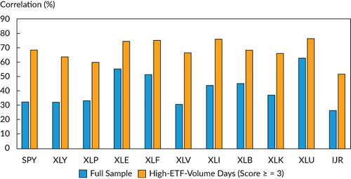
Exhibit 1. ETF Symbols and Names

ETF Symbol	ETF Name
SPY	SPDR S&P 500 ETF
XLY	Consumer Discretionary Select Sector SPDR ETF
XLP	Consumer Staples Select Sector SPDR ETF
XLE	Energy Select Sector SPDR ETF
XLF	Financial Select Sector SPDR ETF
XLV	Health Care Select Sector SPDR ETF
XLI	Industrial Select Sector SPDR ETF
XLB	Materials Select Sector SPDR ETF
XLK	Technology Select Sector SPDR ETF
XLU	Utilities Select Sector SPDR ETF
IJR	iShares Core S&P Small-Cap ETF

How Stock Pickers Can Take Advantage

These correlation abnormalities may have created a plethora of buying opportunities at the security level. To illustrate, we backtested a simple systematic strategy. For each volume spike accompanied by a negative return, we systematically bought the outsiders and held them for 40 days. We did so across all 11 ETFs and across time. We identified outsiders the same way we did in our pharmaceutical and financials case studies: We ranked constituents by ETF beta and built an equal-weighted portfolio of the bottom 10%. Then, to calculate alpha versus the ETF, we levered the portfolio to an ETF beta of 1.0.

Essentially, we replicated our case studies but on a much bigger scale, across a total of 240 volume spikes. All the data we used were out of sample, based on what would have been available at the time. To calculate ETF betas, we used an exponentially weighted regression with a one-quarter half-life (see the online supplemental material, available at www.tandfonline.com/doi/suppl/10.1080/0015198X.2019.1572358).

In Figure 2, we show the average cumulative alpha (the return for the levered outsider portfolio minus the ETF) across all events, from 1 to 40 days after the volume spike and before and after trading costs.¹⁶

Figure 2. Average Alpha after ETF Volume Spike, 4 January 2010–29 December 2017

Notes: Data are as of 29 December 2017. Transaction costs are estimated at 10 bps, or 17 bps considering leverage, on average. Borrowing costs are based on LIBOR and depend on how long the position is held. They cumulate to about 10 bps, on average, after 40 days. Hence, a rough estimate of total costs (transaction and borrowing) for 40 days would be 27 bps.

Sources: S&P; IDC. Data analysis by T. Rowe Price.

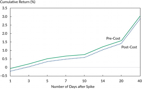
Average alpha on the first post-spike day is slightly negative, which indicates that even if we lagged the implementation time by one day, the strategy would still work. Then, as the time window expands, average alpha cumulates positively and consistently—all the way to 40 days.

In Figure 3, we show average alphas across ETFs and time. The strategy does not work perfectly for all ETFs or at all time horizons, but on average, it generates significant after-cost alpha (see the online supplemental material, available at www.tandfonline.com/doi/suppl/10.1080/0015198X.2019.1572358, for details of the statistical test). Because we force the outsider portfolios’ ETF betas to 1.0, the strategy is not expected to take on any systemic factor exposure—such as market beta, value, or momentum exposures—relative to the ETF. And because we measure performance relative to the ETF, we expect these alphas to be “idiosyncratic” (i.e., stock-picking alphas).¹⁷

Figure 3. Average Alphas after ETF Volume Spike by ETF, 4 January 2010–29 December 2017

Notes: Data are as of 29 December 2017. Transaction costs are estimated at 10 bps, or 17 bps considering leverage, on average. Borrowing costs are based on LIBOR + 50 bps and depend on how long the position is held. They cumulate to about 10 bps, on average, after 40 days. Hence, a rough estimate of total costs (transaction and borrowing) for 40 days would be 27 bps. The Wilcoxon signed-rank test (see the online supplemental material, available at www.tandfonline.com/doi/suppl/10.1080/0015198X.2019.1572358, for details) indicates significance levels of 0.05* and 0.01**. Some returns are positive on Day 0 because they are measured relative to the ETF.

Sources: S&P; IDC; T. Rowe Price.

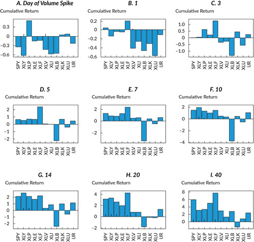
Notably, the strategy did not work well for the Materials Select Sector SPDR ETF (XLB), and although it worked in the short term, it ended in negative territory for the Technology Select Sector SPDR ETF (XLK). These outcomes highlight the risk of systematic, simple trading rules. In these cases, the trading rules led to large positions in low-ETF-beta stocks that underperformed their ETFs after the high-volume selloffs.

Perhaps fundamental analysis would have helped. A stock picker would have analyzed the theme behind each selloff. He would have taken into consideration whether the low-ETF-beta outsiders were truly outsiders to the theme and, if so, whether these companies presented a risk of short-term underperformance for other reasons. Then, he would have scaled the positions relative to the theme according to a risk–return analysis. Once the long positions were established, he would have applied discipline to determine when to sell them, considering market developments and the health of the sector and the companies involved.

Lastly, although the strategy identifies ETF volume spikes and conditions them on down days, it does not condition on the size or duration of the selloff. Focusing on the largest selloffs, with a flexible time horizon, might enhance performance. Volumes across ETFs and index funds also need to be monitored, of course, because several index products may trade in the same sector. Ultimately, a lot more can be done when the strategy incorporates fundamental analysis. Hence, our goal with our simple backtest was to indicate the potential size of the opportunity, not to design a purely systematic approach.

Takeaways

Are ETF investors increasingly at risk of getting “picked off”? Because of the growing popularity—as well as the liquidity and tax benefits—of passive investing, the percentage of trading volume on US exchanges from ETFs has increased significantly. Some ETF investors focus on top-down market views or themes, whereas others believe that markets are efficient and simply want broad index exposures. In all cases, when they trade, most ETF investors—and index investors in general—ignore security-level fundamentals. They simply buy or sell all securities in the index in proportions determined by the index provider (typically, market-capitalization weights).

As a result, we find that when ETF volumes spike, correlations among constituents increase to levels that are not justified by company-level fundamentals. Our study of 240 events since 2010, compiled across 11 ETFs, suggests that these correlation bubbles may create opportunities for stock pickers. Investors who buy oversold constituents after high-ETF-volume days and hold them as they mean-revert over the next 5 to 40 days may generate alpha at the expense of index investors. Are we witnessing the revenge of the stock pickers?

Ultimately, there’s a place for both passive and active investors in markets. ETF investors and stock pickers can happily coexist. We report gains for stock pickers that are of practical significance, but these results don’t mean ETFs are bad. They simply mean that different investors can make markets more liquid and efficient together. Market efficiency remains a paradox: Profit opportunities, such as the one we have identified (and which indicate inefficiencies), are necessary to make markets more efficient. Such are the ebbs and flows of financial market equilibrium.

Acknowledgments

The authors would like to thank Dave Eiswert, Henry Ellenbogen, and Mark Vaselkiv for examples of the impact of ETF volume spikes on abnormal constituent correlations and Prashant Jeyaganesh for help with data. We are also grateful for comments and support from Sudhir Nanda, Rob Sharps, and Bill Stromberg.

Notes

¹ Robin Wigglesworth, “ETFs Are Eating the US Stock Market,” Financial Times (24 January 2017). Volume data are from Credit Suisse, as of 2016. Interestingly, in 2016, 7 of the 10 most traded securities were ETFs, not stocks. And the Wall Street Journal reports that the ETF industry has grown to $3.5 trillion in size: Asjylyn Loder, “Investors Win from ETF Price War,” Wall Street Journal (12 July 2018). www.wsj.com/articles/etf-fees-tumble-as-price-war-heats-up-among-big-fund-firms-1531396800.

² In a related article, Chao, Shah, Finelli, Martin, Okoro, Jalagani, Zhao, and Elledge (2018) showed that a contrarian strategy that buys stocks with high ETF outflows and sells stocks with high ETF inflows generates substantial profits.

³ For an extreme example, the case of the VanEck Vectors Junior Gold Miners ETF is interesting. See Asjylyn Loder and Chris Dieterich, “How a $1.4 Billion ETF Gold Rush Rattled Mining Stocks around the World,” Wall Street Journal (23 April 2017). The authors mentioned that “money rushing into exchange-traded funds investing in gold mining stocks sparked wild trading in the stocks while the price of gold was largely flat.”

⁴ Notably, the authors didn’t find this same increase in informational efficiency “for big firms, stocks with high analyst following, and for stocks with perfectly competitive equity markets” (3). With the exception of IJR (the small-cap ETF), all 10 of our other ETFs are made up of firms in the S&P 500, which are generally “big firms” with “high analyst following.”

⁵ Percentiles calculated for all seven-day periods from 22 December 1998 to 28 September 2015.

⁶ https://twitter.com/hillaryclinton/status/645974772275408896?lang=en.

⁷ Andrew Pollack, “Drug Goes from $13.50 a Tablet to $750, Overnight, “ New York Times (20 September 2015). www.nytimes.com/2015/09/21/business/a-huge-overnight-increase-in-a-drugs-price-raises-protests.html.

⁸ Valeant actually began trading under the name Bausch Health Companies Inc. on Monday, 16 July 2018.

⁹ It could be argued that drug-pricing pressures could ultimately affect the entire medical system and thereby impact medical equipment providers. However, these stocks’ reaction still seems exaggerated.

¹⁰ Throughout this article, including in the 2010–17 backtest, transaction costs are estimated at 10 bps, or 17 bps considering leverage (on average). Borrowing costs are based on LIBOR + 50 bps and depend on how long the position is held. They cumulate to about 10 bps on average after 40 days. Hence, a rough estimate of total costs (transaction and borrowing) for 40 days would be 27 bps.

¹¹ Zacks Equity Research, “Stock Market News for February 11, 2016,” NASDAQ (11 February 2016). www.nasdaq.com/article/stock-market-news-for-february-11-2016-cm578585.

¹² Larry Elliott and Jill Treanor, “Stock Markets Hit by Global Rout Raising Fears for Financial Sector,” Guardian (11 February 2016). www.theguardian.com/business/2016/feb/11/stock-markets-hit-by-global-rout-raising-fears-for-financial-sector.

¹³ Ben Levisohn, “American Express: No, Higher Interest Rates Won’t Help,” Barron’s (22 December 2016). www.barrons.com/articles/american-express-no-higher-interest-rates-wont-help-1482422718.

¹⁴ Zacks Equity Research, “Stock Market News for February 11, 2016,” NASDAQ (11 February 2016). www.nasdaq.com/article/stock-market-news-for-february-11-2016-cm578585.

¹⁵ ETF volumes have steadily increased over time. Although ETF data are available starting in 1998, we start our data sample in January 2010, which is about when ETF trading volumes became meaningful on a sustained basis. In 2010, the proportion of shares held by ETFs reached 2.5%, and by 2014, it had grown to 4% (see Da and Shive 2018). We also studied the pre-2010 period and found weaker effects of ETF volume spikes on correlations, as expected (details available upon request). We think this regime shift is meaningful and reflects the effect of the growing popularity of passive investing during the more recent period.

¹⁶ Our choice of the 1- to 40-day windows is motivated by prior studies, as well as the need to avoid too many overlapping events. Ben-David et al. (2018) found that “most of the contemporaneous stock-price effect of ETF flows reverts over the next 40 days, in line with the view that the demand shocks in the ETF market translate into nonfundamental price changes for the underlying securities” (2473). Brown et al. (2018) used a one-month horizon. While extending the window beyond 40 days is possible (and we have found that alpha continues to accumulate after 40 days), it creates too many overlapping events and makes it more difficult to attribute alpha. Note that the median number of days between ETF spike dates in our sample is 38.

¹⁷ In line with this intuition, Brown et al.’s (2018) analysis shows that ETF-driven reversals generate significant alphas after controlling for the Fama–French three factors plus momentum. Using betas calculated over the 252 pre-event days, the expected beta to the S&P 500 was slightly higher for the levered outsider portfolio than it was for the ETF. Consequently, after adjusting for the exposure to the market in the 40 post-event days, we could see a reduction in the alpha generated by our strategy of about 20 bps—a fraction of our 300 bps of pre-cost alpha. We leave it to the reader to interpret whether this slight excess beta constitutes a systematic bias, but if so, the impact remains small relative to the magnitude of the net alphas. Regarding liquidity, our outsiders have a similar liquidity profile, on average, to their peer constituents. And the distribution is symmetrical: Roughly half the low-ETF-beta stocks have above-average liquidity, and half have below-average liquidity.

References

- American Express Company2015. “2015 American Express Company Annual Report.” https://ir.americanexpress.com/Cache/1500081626.PDF?O=PDF&T=&Y=&D=& FID=1500081626&iid=102700.
- Barberis, Nicholas, Andrei Shleifer, and Jeffrey Wurgler. 2005. “Comovement.” Journal of Financial Economics, vol. 75, no. 2: 283–317.
- Ben-David, Itzhak, Francesco A. Franzoni, and Rabih Moussawi. 2018. “Do ETFs Increase Volatility?” Journal of Finance, vol. 73, no. 6: 2471–535.
- Brown, David C., Shaun Davies, and Matthew C. Ringgenberg. 2018. “ETF Flows, Non-Fundamental Demand, and Return Predictability.” Working paper (November) .
- Cahan, Rochester, Yu Bai, and Sungsoo Yang. 2018. “The ETF Selection Model—Don’t Pick the ETF, Pick the Stocks in the ETF.” Empirical Research Partners14 (February) .
- Chao, Alex, Ronnie Shah, Pam Finelli, Hallie Martin, Chin Okoro, Srineel Jalagani, George Zhao, and David Elledge. 2018. “What Happens When the World Goes Passive? Active ETF Flow Strategies.” Deutsche Bank Research, Quantitative Strategy16 (July) .
- Da, Zhi, and Sophie Shive. 2018. “Exchange Traded Funds and Asset Return Correlations.” European Financial Management, vol. 24, no. 1: 136–68.
- Giamouridis, Daniel. 2017. “Systematic Investment Strategies.” Financial Analysts Journal, vol. 73, no. 4: 10–14.
- Glosten, Lawrence R., Suresh Nallareddy, and Yuan Zou. 2016. “ETF Activity and Informational Efficiency of Underlying Securities.” Columbia Business School Research Paper No. 16-71 (December) .
- Greenwood, Robin M., and Nathan Sosner. 2007. “Trading Patterns and Excess Comovement of Stock Returns.” Financial Analysts Journal, vol. 63, no. 5: 69–81.
- Hill, Joanne. 2016. “The Evolution and Success of Index Strategies in ETFs.” Financial Analysts Journal, vol. 72, no. 5: 8–13.
- Madhavan, Ananth, and Daniel Morillo. 2018. “The Impact of Flows into Exchange Traded Funds: Volumes and Correlations.” Journal of Portfolio Management, vol. 44, no. 7: 96–107.
- Page, Sebastien, and Robert A. Panariello. 2018. “When Diversification Fails.” Financial Analysts Journal, vol. 74, no. 3: 19–32.
- Sullivan, Rodney N., and James X. Xiong. 2012. “How Index Trading Increases Market Vulnerability.” Financial Analysts Journal, vol. 68, no. 2: 70–84.
- Wurgler, Jeffrey. 2010. “On the Economic Consequences of Index-Linked Investing.” NBER Working Paper 16376 (September) .