Reports of Value’s Death May Be Greatly Exaggerated

Abstract

Value investing, as defined by the Fama–French high book-to-market minus low book-to-market (HML) factor, has underperformed growth investing since 2007, producing a drawdown of 55% as of mid-2020. The underperformance has led many market observers to argue that value is dead. Our analysis attributes value’s recent underperformance to two sources: (1) The HML book-value-to-price definition fails to capture increasingly important intangible assets, and (2) valuations of value stocks relative to growth stocks have tumbled. Both observations are inconsistent with the argument for value’s death. We capitalize intangibles and show that this measure of value outperforms the traditional measure by a wide margin. We also describe a return decomposition and demonstrate that changes in the valuation spread between the growth and value portfolios explain the entire drawdown, with room to spare. The relative valuation of the value factor falls from the top quartile of the historical distribution at the start of 2007 to the bottom percentile as of June 2020

Disclosure: Research Affiliates, LLC, has a commercial interest in the subject matter.

Editor’s Note:

Submitted 3 June 2020

Accepted 21 October 2020 by Stephen J. Brown.

This article was externally reviewed using our double-blind peer-review process. When the article was accepted for publication, the authors thanked the reviewers in their acknowledgments. Andrew L. Berkin and one anonymous reviewer were the reviewers for this article.

Correction: This article was originally published with a production error in Figure 1B and endnote 32, which have now been corrected in the online version. Please see Correction ( https://doi.org/10.1080/0015198X.2021.1895584).

View correction statement:

Correction

An investment strategy, style, or factor can suffer a period of underperformance for many reasons.

• The style may have been a product of data mining and worked during its backtest only because of overfitting.

• The trade may get crowded, which distorts asset prices and leads to low or negative expected returns.

• Structural changes in the market may render the factor newly irrelevant.

• Structural changes in the economy may make a particular accounting-based expression ineffective in capturing the factor premium.

• Recent performance may disappoint because the style or factor is becoming cheaper as the factor reaches new lows in relative valuation.

• Finally, flagging performance may be a result of a left-tail outlier or simple bad luck.

The first three reasons (among others) might imply the style no longer works, but the last three reasons have no such implications.

Many investors are reexamining their exposure to value investing because of the extraordinary span of underperformance—from 2007 to mid-2020, and counting—relative to growth investing. In that period, the standard high book-to-market minus low book-to-market (HML) factor based on the book-to-price ratio (B/P) of Fama and French (1993) experienced a drawdown of –55%. As of June 2020, the current drawdown is the largest drawdown observed since June 1963.¹ Given the long historical record of value investing and its solid economic foundations (dating back to the 1930s and, less formally, dating back centuries), the strong performance up to 2007 is unlikely to have been a result of overfitting.

Our analysis suggests that the last three reasons have contributed the most to value’s travails. Specifically, we observe that B/P, in the standard value definition, tends to misclassify stocks as value and growth by failing to capture a company’s investments in intangible assets. Furthermore, in the last 13½ years, the relative valuation of value stocks in relation to growth stocks has become cheaper than ever before in history.² Just as a stock may become cheap relative to its fundamentals, so may an investment style, strategy, or factor. As it becomes cheaper, its performance is poor, but that weak performance has nothing to do with future performance; indeed, if any mean reversion occurs in valuations, the poor performance may presage excellent future results. Because the relative valuation for the value factor has reached the lowest levels of the last 57 years, eclipsing even the depth of the tech bubble in 2000, this revaluation is by far the largest contributor to value’s underperformance. Finally, part of the underperformance cannot be distinguished from an extreme left-tail event.

We start our analysis with an examination of the question of the adequacy of the P/B measure to capture the value effect in today’s economic environment. The economy has rapidly moved from agriculture to manufacturing to a service and knowledge economy. Therefore, we have economic reasons to believe that simple measures of value, such as B/P, are problematic. For example, a company presumably undertakes the creation of intangibles (e.g., research and development, patents, and intellectual property) because the managers expect these investments to enhance shareholder value. These investments are typically treated as an expense, however, and are not accounted for as amortizable assets on the balance sheet, which effectively lowers—we would argue understates—book value by the amount invested in the intangibles. The fact that some of these investments in intangibles fail to deliver future profits is no different from an oil company drilling a dry hole or a new manufacturing plant becoming obsolete before it can turn a profit. Mistakes are a normal part of the business world. The current accounting treatment leads the stocks of many companies to be classified as growth stocks because of low—sharply understated—book values. Many of these stocks would have been classified as neutral or value stocks if the value of the internally generated intangible investments had been capitalized, thus increasing book value.

Penman and Reggiani (2018) suggested that book to market is not a sufficient statistic for determining whether an investor invests in value or growth: “When applied jointly with E/P, high B/P . . . indicates higher future earnings growth” (p. 104). That is, a strategy that looks like a value strategy sometimes tilts toward growth. Lettau, Ludvigson, and Manoel (2019) suggested that the issue identified by Penman and Reggiani is important for the asset management industry. Lettau et al. showed that of the funds that call themselves “value funds,” few rely on B/P to define value. According to the B/P definition, many of the funds hold more growth stocks than value stocks in their portfolios.³

In the absence of an agreed-upon industry-wide measure of value, selecting a single measure, such as B/P, for use in valuation may be unwise, especially when a company’s book value is a materially incomplete measure of its financial position. Also, capitalizing intangible investments makes sense to have a realistic measure of a company’s capital. Our empirical work shows that if companies had capitalized these intangibles, the average annual return of the standard HML factor would have improved by 2.2 percentage points (pps) per year since 2008. Our results, together with those of Lettau et al. (2019), imply that some value funds performed surprisingly well during value’s current drawdown because in due course, they adjusted their approach away from a flawed definition.

Next in our analysis, we explore the influence of relative valuations on the recent value drawdown. The performance of value versus growth naturally disaggregates into three components: revaluation, migration, and income yield. Revaluation is the change in the relative valuation of growth versus value. If growth stocks become more expensive relative to value stocks, the mere process of value becoming cheaper relative to growth means that value underperforms growth. Indeed, revaluation accounts for about two-thirds of the variability in factor returns over the past 13½ years and well over 100% of the cumulative shortfall. This result is not particularly surprising given that six stocks, which we describe as the “FANMAG” stocks, have collectively appreciated more than tenfold since 2007. ⁴ These six stocks represented about 20% of US stock market capitalization and 32% of the Fama–French large-cap growth portfolio as of 30 June 2020. Without the FANMAGs, the performance of the S&P 500 Index over the same period would have cumulatively been more than 3,000 bps lower. None of these stocks is a value stock.

The two other performance components are also important. Migration occurs when value stocks appreciate (leading to a lower B/P) and no longer qualify for the value portfolio and when growth stocks falter (leading to a higher B/P) and no longer qualify for the growth portfolio. Because value strategies underweight or short growth stocks, an underperforming growth stock enhances these strategies’ returns. Migration markedly boosts the performance of value versus growth. Migration also boosts the book value of the value portfolio and lowers the book value of the growth portfolio every time these portfolios are rebalanced. The reason is that a no-longer-cheap value stock is kicked out of the value index and replaced with a newly cheap stock, which is trading at a higher B/P. Similarly, a growth stock that has fallen out of favor is replaced with a new high flyer, which sports a much lower B/P. ⁵

Income yield is the third driver of relative performance because most growth stocks are more profitable and exhibit faster growth in sales and profits than most value stocks. Income yield benefits growth relative to value and offsets much—but, typically, not all—of the benefit from migration. We consider migration and income yield to be structural drivers of the value premium. When we compared pre-2007 data with post-2007 data, we found little evidence of any meaningful change in the performance attributable to migration or income yield.

We then sought to measure the structural premium of the value strategy by purging the revaluation component from the value-minus-growth return. Specifically, in 2007, the valuation spread (value minus growth) was narrow, in the top quartile (25th percentile). By June 2020, the spread had widened to an unprecedented extent, with the value portfolio at its all-time cheapest level since 1963 (100th percentile) relative to growth. When value becomes cheaper relative to growth, value stocks underperform growth stocks. The residual return, which we term the “structural return,” is a combination of the income yield difference favoring growth and migration favoring value.

Our analysis subsumes a number of potential explanations for value’s underperformance. For example, some have said that the value trade has become crowded, distorting stock prices so the factor generates a tiny or negative expected return. Crowding should cause the factor to become more richly priced. An increase in the valuation spread between growth and value, from the 25th to the 100th percentile, however, is not consonant with crowding into the value factor. Thus, this narrative is easy to dismiss. ⁶

Similarly, little evidence exists to suggest that the value strategy’s long-run structural return has turned negative or even diminished from the pre-2007 level. The main difference between now and then is the rise in valuations, both for growth relative to value and for US stocks in general. Unless we choose to assume that the valuation spread between value and growth stocks will continue to widen indefinitely, our analysis suggests that value is highly likely to outperform growth in the years ahead.

Our results relate, in particular, to those of Lev and Srivastava (2019), who suggested that value investing has been unusually unprofitable not only during the current drawdown but for as long as 30 years. They concluded, similarly to us, that one of the reasons for the underperformance is the accounting treatment of investments in intangible assets as expenses.

Value’s Recent Travails

The value strategy as a systematic approach to equity investing dates back at least to the 1930s. Graham and Dodd (1934), in their classic Security Analysis, laid down the main principles of value investing. By comparing the intrinsic value (capturing the future discounted stream of a company’s cash flows) and the market’s value of a company, investors can identify good buying and selling opportunities, which is the core of the value investing process. Basu (1977) was one of the first to empirically document a value premium by demonstrating that value stocks, defined as having a high earnings-to-price ratio (E/P), outperform growth stocks, defined as having a low E/P. In the following decades, multiple research papers showed that almost any definition of value that uses a fundamentals-to-price ratio produces a comparable return difference between value and growth stocks. ⁷ Following the studies by Fama and French (1992, 1993), the academic consensus settled on the B/P as the leading definition of value.

The source of the value premium is controversial. One camp, led by Fama and French (1992, 1993), views the premium as compensation for bearing risk; the other camp, led by Lakonishok, Shleifer, and Vishny (1994), argues that mispricing drives the premium. Although disagreement surrounds the source of the premium, most agree that the premium exists and is not an artifact of a data-mining exercise. Indeed, the value effect is present in most asset classes (Asness, Moskowitz, and Pedersen 2013), is robust to perturbations in definition, and does not require high transaction costs to execute (Beck, Hsu, Kalesnik, and Kostka 2016).

Table 1 shows the performance characteristics of the value factor compared with a handful of other popular factors. To define this factor, we used the Fama–French method, which equally weights large- and small-cap stocks.⁸ We constructed two portfolios—one consisting of the highest 30% and the other, the lowest 30% of the market chosen by B/P—and weighted each portfolio by market capitalization. Then, we examined the difference in the performance of the two portfolios. We compared this “factor performance” with the performance of other leading factors, many of which are constructed along similar lines but use measures other than B/P to differentiate the favored stocks from the less favored. Over the 1963–2020 period of our analysis, even inclusive of the 13½-year drawdown, value remained one of the most impressive factors in terms of risk–return characteristics. Only momentum had better performance over the full span, and that result does not take trading costs into account (momentum has immense turnover).

Table 1. Major Factor Performance, US Stocks

		July 1963–June 2020					January 2007–June 2020
Factor	Year of Discovery	Average Return	St. Dev.	t-Stat.	CAPM α t-Stat.		Average Return	St. Dev.	t-Stat.	CAPM α t-Stat.
Market	1964	6.5%	15.4%	3.17			8.6%	15.9%	1.99
Value	1977–90	3.0	9.8	2.34	3.12		–5.4	9.9	–2.00	–2.64
Size	1975	2.2	10.3	1.63	0.70		0.0	8.0	–0.01	–0.83
Profitability	2013	2.8	7.7	2.77	3.55		3.2	5.6	2.08	2.81
Investment	2003	2.5	6.3	3.00	4.36		–0.6	4.8	–0.48	–0.38
Momentum	1989	7.8	14.5	4.04	4.57		1.2	16.4	0.27	1.13
Low beta	1966	0.2	15.4	0.10	3.47		–2.7	16.4	–0.62	1.22

Notes: All returns are for long–short strategies based on factors (similar to the HML factor of Fama and French). Reported are both the t-statistics for the return of the long–short portfolios and the t-statistics for the corresponding CAPM alphas. Because the capital asset pricing model (CAPM) adjusts for market risk and given that many of the factors had negative market betas in the 1963–2020 period, the t-statistics associated with CAPM alphas tend to be higher than those for simple returns. The adjustment for market risk is particularly important for the low-beta factor. This factor’s average return is close to zero, but given its negative market beta, it has a statistically significant CAPM alpha. The long–short factor has a negative market beta because the long side contains stocks with below-1.0 market betas and the short side contains stocks with above-1.0 market betas. We used the Fama and French (2015) definition for the investment and profitability factors (where the profitability factor was initially popularized by Novy-Marx 2013). We also followed the definition of the momentum factor from the website of Kenneth French: https://mba.tuck.dartmouth.edu/pages/faculty/ken.french/data_library.html. The momentum factor was first documented by Jegadeesh and Titman 1993; it was popularized by Asness 1994 and Carhart 1997 as part of factor models.

Sources: Research Affiliates, LLC, using data from CRSP/Compustat.

Since the beginning of 2007, the value factor appears to have reversed its previous course of strong performance.⁹ A portfolio of value companies (based on the Fama–French high-B/P criterion) held from July 1963 through December 2006 and rebalanced annually to maintain a focus on value stocks would have grown to 9.5 times the value of a portfolio of low-B/P growth companies held over the same period, before the value portfolio contracted 55% by the end of June 2020.¹⁰ Although the value investor’s wealth tumbled by 55% relative to the growth investor’s wealth in the 13½ years since the start of 2007, the value investor is still 4.3 times as wealthy as the growth investor for the period July 1963–June 2020.

Table 2 describes the three deepest and three longest value drawdowns in our 57-year sample. The current drawdown, which is still unfolding, is the deepest. At –54.8%, it has eclipsed the tech bubble, which at its bottom had a drawdown of –40.6%.¹¹ The current drawdown span of 13½ years is (by a wide margin) the longest-lasting period of value underperformance. The second longest-lasting period of value underperformance was the biotech bubble in the early 1990s, which lasted for a much shorter period—3 years and 7 months from peak to trough to new high. That said, if we narrow our focus to large-cap stocks, for which the value effect is generally weaker, we found two back-to-back drawdowns—the biotech bubble and the tech bubble—interrupted by a scant one-month new high. Combine these two, and this earlier drawdown lasted 11 years and 10 months and left large-cap value investors more than 39.4% poorer than growth investors. This immense shortfall was recovered (requiring over 65% outperformance) in just 13 months.

Table 2. US Value Stocks vs. US Growth Stocks: Worst Value Drawdowns, July 1963–June 2020

		Dates
Rank	Event	Start Date	Bottom	End Date	Length	Drawdown
A. Deepest drawdowns
1	Current	2006/12	2020/06	—	13 yrs., 6 mos.	–54.8%
2	Tech bubble	1998/08	2000/02	2001/02	2 yrs., 5 mos.	–40.6
3	Iran oil crisis	1979/07	1980/11	1982/02	2 yrs., 6 mos.	–28.2
B. Longest-lasting drawdowns
1	Current	2006/12	2020/06	—	13 yrs., 6 mos.	–54.8%
2	Biotech bubble	1989/06	1991/12	1993/02	3 yrs., 7 mos.	–24.9
3	Nifty Fifty*	1970/08	1972/06	1973/04	2 yrs., 7 mos.	–17.1
C. Deepest drawdowns, large-cap only
1	Current	2007/03	2020/06	—	13 yrs., 2 mos.	–61.1%
2	Biotech/tech bubble**	1989/03	2000/02	2001/03	11 yrs., 10 mos.	–39.4
3	Nifty Fifty	1969/01	1972/07	1973/12	4 yrs., 10 mos.	–25.1

*The Nifty Fifty was a (somewhat changing) group of roughly 50 large-cap stocks on the NYSE characterized by their consistent earnings growth, high price-to-earnings ratios, and other valuation multiples in the late 1960s and early 1970s. They were originally touted as stocks worth buying at any valuation. Subsequently, these stocks generated disappointing returns for investors (despite often fantastic business successes).

**Biotech recovered from the previous peak by 0.3% in the single month of July 1993 before the drawdown associated with the tech bubble started.

Sources: Research Affiliates, LLC, using data from CRSP/Compustat.

Is the current value drawdown an “unlucky” outcome in line with previous drawdowns, or is this time truly different? Specifically, if we use the pre-2007 characteristics of value for guidance, should we be shocked to see a drawdown of –54.8% at some stage during a 57-year span?

We used a block bootstrap simulation following Arnott, Harvey, Kalesnik, and Linnainmaa (2019) to answer this question. In the simulation, we resampled the value factor returns by drawing random six-month blocks of actual long–short HML factor returns from the live historical sample from July 1963 through December 2006. We used the six-month blocks to preserve some of the autocorrelation structure of the return-generating process. Note that we ended the historical sample in the last month before the current drawdown began, thereby excluding the recent drawdown. We were asking whether prior data might have led us to believe that the protracted drawdown since 2007 was a plausible outcome.

Each simulated sample is 57 years long to match the length of the history from July 1963 through June 2020. We repeated this exercise 1 million times. In so doing, we generated 1 million alternative histories based on random draws from HML value-versus-growth relative returns. We then measured the size of the largest drawdown in each simulated sample. We were seeking to ascertain how many of the million simulated histories had a drawdown comparable to the –54.8% decline from January 2007 through June 2020.

The bootstrap simulation (see Appendix A) shows that the median outcome was a –32.7% drawdown and that a drawdown larger than the latest one—a –54.8% drawdown—occurred in 2.3% of our simulations. Although this result meets standard definitions of statistical significance, the analysis is deliberately biased toward a low probability: We specifically excluded the recent drawdown from the data we used in the bootstrap simulations and ran this test specifically because of the drawdown.

Is This Time Different?

The recent value underperformance raises a reasonable question: Is this time different? Put another way, is this disappointment a new normal for value investors? Is the value premium gone—or even negative? Many narratives are being offered to suggest that value investing no longer has merit. They generally fall into one of the following categories. The first two (overfitting and crowded trades) are the simplest and the easiest to dismiss. The next five are structural changes in the economy that, ostensibly, make the value factor newly irrelevant. None of these narratives fares particularly well in empirical testing.

The final three are the most important and are demonstrably accurate: (1) Intangibles are not captured by book value, so the B/P-based HML factor is a poor way to distinguish between growth and value; (2) a widening valuation spread between growth and value simultaneously pushes down the past performance for HML and, with value now at the cheapest relative valuation in history, pushes up the likely future performance; and (3) we have a left-tail extreme outlier, in both current relative valuation and recent relative performance. We will return to these narratives after briefly reviewing the narratives that have less merit. We propose a return decomposition that suggests that intangibles, revaluation, and a left-tail outlier are all important elements of value’s travails. The evidence for the other narratives is weak. It is beyond the scope of this article to test all the narratives, but our approach addresses the most important empirical predictions for all of them.

Was Value Merely Lucky in the Past, or Is It Now Arbitraged Away by Its Own Popularity?

This question brings up the first two explanations—the simplest and the easiest to dismiss.

Overfitting.

A particular strategy may have been a product of data mining discovered by multiple testing and with analysts working only in the backtest as a result of overfitting.¹² Given the amount of evidence, the economic theory, and the long investment management practice behind value investing, this explanation is doubtful, and it is further contradicted by the still-positive structural return for the HML value factor net of revaluation.

Crowded trade.

Value is a popular factor that is widely accepted as a legitimate factor throughout the academic and factor-investing communities. Smart beta and its cousin, factor investing, have been among the fastest-growing strategies in the past decade. They have attracted, by some measures, US$1 trillion or more (per Morningstar). These flows have ostensibly led to crowding, so the value factor may have been “arbitraged away.” If the crowding narrative were correct, then the value premium would be structurally impaired for as long as crowding persists. Value investors’ trades should boost the prices (and valuation multiples) of value companies, relative to those of growth companies, to a point where the income yield and migration effects exactly cancel. The opposite has happened: Value has become cheaper relative to growth, to an unprecedented extent.

Have Structural Changes in the Economy Made the Value Factor Newly Irrelevant?

Here we turn to the explanations that have some merit.

Technological revolution, hence better growth stocks.

This narrative suggests that today’s growth stocks are growing faster and earning more profit than the growth stocks of the past. In the decade between 2010 and now, we witnessed the emergence of a vast digital sector that is leveraging technological prowess to take over large parts of the macroeconomy. The recent success stories of the FANMAG stocks are captivating. These enterprises have driven many established companies out of business. The US-based tech companies are collectively vastly profitable. The combined capitalization of the FANMAG stocks was US$6.15 trillion in mid-2020, exceeding the stock market capitalization of every country in the world except that of the United States and China. These six stocks are worth more than the entire publicly traded economy of such economic powerhouses as Japan, the United Kingdom, and Germany. This explanation suggests that the disruptive new technological leaders can drive outsized monopolistic profits that choke the old brick-and-mortar value companies into irrelevance.

If this narrative is correct, then value investing may be structurally impaired for a prolonged period of time. Empirically, we should expect that growth companies will have already become even more profitable and faster growing relative to value companies than they were historically. The evidence contradicts this thesis.

Less migration.

We hear that migration may be slowing for several reasons. For instance, the structure of many industries is more monopolistic than it was a few decades ago, which makes it harder for new companies to gain market share. Also, as the valuations of growth and value diverge, for companies to migrate from growth to value, and vice versa, becomes more difficult. A related argument suggests that both the markets and the economy have evolved to a point where value stocks stay cheap and growth stocks stay richly priced, slowing the migration that drives the value advantage. The more stable valuations could also be driven, in part, by market participants’ increased sophistication, which allows investors to “get it right” on the relative valuations of most companies more often than in the past.

If any of these narratives is correct, then we should observe a lower portion of value’s return attributed to the change in style (i.e., value stocks migrating toward growth and growth stocks migrating toward value). Empirically, we found that migration is essentially unchanged from the past.

Low interest rates.

Since 2008, we have witnessed a period of zero or near-zero interest rates—which has no historical precedent. US$11.6 trillion of government bonds worldwide were trading at negative yields at the end of June 2020. ¹³ In the standard Gordon formulation, low interest rates should have a disproportionate valuation impact on the longer-duration and lower-yielding assets, unless the low interest rates are being driven by a drop of similar magnitude in growth expectations. Liu, Mian, and Sufi (2019) suggested that industry leaders can disproportionately benefit from low interest rates to generate outsized monopolistic profits.

The implications and empirical predictions of this narrative are similar to those suggested by the technological revolution narrative, although the economic mechanism is different. Arnott, Harvey, Kalesnik, and Linnainmaa (2020) showed, however, that over the 1926–2020 period, no meaningful relationship existed between interest rate levels, or changes in rates, and the value premium. In addition, they documented that value companies benefit more from low interest rates than growth companies because they often carry more debt than growth companies.

Stranded assets (assets prematurely written down, devalued, or converted to liabilities).

The market value of an enterprise reflects the value of the future use of the assets owned by the enterprise. As the economy and regulations evolve, certain types of assets may significantly depreciate in value or become associated with material future liabilities. Particularly, as environmental, social, and governance (ESG) issues rise to the top of the public’s and regulators’ concerns, the old business models of energy, tobacco, gambling, and many other types of companies—overwhelmingly value stocks—may take a strong hit. Although the ESG conversation is as important and influential as it has ever been, it is merely another form of creative destruction that has been with us since the dawn of civilization and that almost always afflicts value stocks relative to growth stocks.

Growth of private markets.

The number of US listed stocks has more than halved in just 23 years, from more than 7,500 in 1997 to barely 3,600 today.¹⁴ There are many reasons for the decline (not least being the regulatory environment for publicly traded companies), but one narrative suggests that part of the decline may result from the growth of private equity investors who buy potentially undervalued stocks and take them out of the public markets. Such activity leaves fewer value opportunities in the markets and potentially lowers the expected return on value.

This narrative suffers from two logical inconsistencies. First, most private equity investors are seeking growth, not value. Second, given the growth of private equity, the buying pressure should increase the prices of deep-value stocks when they become, and are, private equity targets. So, on the one hand, some stocks that would fall into the value portfolio may disappear, but on the other hand, the activities of private equity investors should elevate the prices of certain value stocks before they disappear.

Now consider the narratives that demonstrably have merit.

The trouble with intangibles.

The book-to-price ratio is only one of many ways to define value. Intrinsic value is another definition, one introduced by Graham and Dodd (1934). Indeed, they specifically cautioned against the use of B/P as a substitute for intrinsic value.¹⁵ In today’s economy, this warning is even more relevant than it was in the 1930s; today, companies’ intangible assets—intellectual property, patents, brands, software, human capital, reputational capital, customer relationships, and so forth—are often at the core of their ability to generate and maintain profit margins, yet these aspects are almost totally ignored by the accounting for book value. Book value captures only the traditional tangible capital locked in bricks and mortar and in financial assets, such as cash and other securities. If a company spends US$1,000 on a new desk, under Generally Accepted Accounting Principles (GAAP), book value is unchanged; the financial assets are converted into fixed assets and decline over time as assets depreciate. If a company invests US$1 billion in research and development (R&D), the book value decreases immediately by US$1 billion. ¹⁶

From an accounting viewpoint, book value can capture the value of intangibles only through contributed capital, or goodwill, in a corporate acquisition. ¹⁷ If a company spends US$1 billion on R&D, the book value decreases, but if a company spends US$1 billion to purchase another company with US$1 billion worth of evaluated goodwill or other intangible assets, the acquisition target’s investment in R&D shows up in book value. This process makes the B/P vulnerable to misclassifying intangibles-heavy companies as expensive because book value understates the company’s assets as long as the company seeks to grow organically rather than through acquisition. Reciprocally, book value can misclassify intangibles-light companies as cheap. Is a better, more objective measure of a company’s assets, including its intangibles, possible?

Suppose we have a company that invests in R&D and selling, general, and administrative (SG&A) expenditures because we expect to earn that money back within a reasonable time span. Accordingly, following Peters and Taylor (2017), we capitalize all R&D expenditures as knowledge capital and apply a 30% share of SG&A expenditures as capital related to human capital, brand development, and a distribution network.¹⁸ Suppose these sums are added to book value, rather than expensed, much as if the expenditures were used to buy a building, and then amortized away over a suitable span. (After all, no one will buy a building or invest in R&D unless they expect this investment to be profitable within a reasonable time.) After we capitalize both R&D and 30% of SG&A expenses, we then amortize those expenses, much as a building is depreciated, with the perpetual inventory method used by Peters and Taylor.¹⁹

Panel A of Figure 1 plots a marketwide average measure of the importance of intangibles, relative to a company’s tangible book value of equity (financial assets plus physical assets minus debt). We considered all intangibles—the purchased intangibles that show up in book value plus capitalized R&D and SG&A—as compared with book value after we excluded the purchased intangibles. The aggregate of all intangibles is summed across all companies in the US market as the numerator, and the book value minus purchased intangibles (typically goodwill) is summed across all companies as the denominator of the ratio. The history of this ratio from mid-1963 to mid-2020 is shown in Panel A as averaged across the whole US equity market and then separately for the Fama–French growth and value portfolios (selected on the traditional basis of B/P, not intangibles-adjusted B/P).²⁰ The increasing importance of intangibles for growth stocks, but not for value stocks, is self-evident.

Figure 1. Ratio of Various Definitions of Intangibles to Book Value of Equity: US Market, 1963–2020

Notes: Panel A displays the ratio of all intangibles (capitalized R&D and 30% of SG&A plus acquired intangibles) to the tangible part of the book value of equity (the book value of equity minus acquired intangibles). Panel B displays the ratio of internally generated intangibles (capitalized R&D and 30% of SG&A) to the book value of equity.

Sources: Research Affiliates, LLC, using data from CRSP/Compustat; Peters and Taylor (2017).

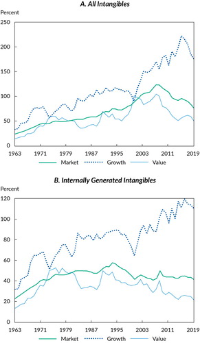
Panel B of Figure 1 shows intangibles from a perspective that will be intuitive to the practitioner community; it shows how much book value goes up if we capitalize R&D and capitalize 30% of SG&A (we refer to the sum of capitalized R&D and SG&A expenses as “capitalized intangibles”). As with Panel A, we measured the sum total of capitalized intangibles, as our numerator, and the sum total of book value for all companies, as our denominator. The sample excludes companies with negative book values of equity or missing market values of equity. We report this ratio for the market and for the Fama–French growth and value portfolios from 1963 to 2020. The graph in Panel B clearly shows that the intangibles that are missing from book value are soaring in importance on the growth side of the market.

As Panel A of Figure 1 shows, in 1963, intangibles were just 25% of the tangible portion of book value for the US stock market as a whole. By the mid-1970s, that figure had doubled, and by the early 2000s, it had doubled again. This ratio has remained around 100% ever since. The more interesting result is the divergence between growth and value. Since about 2015, the average value of all intangibles (including purchased intangibles) has been only about half as large as the tangible book value for value stocks and about twice as large as the tangible book value for growth stocks.

As shown in Panel B of Figure 1, in 1963, if R&D and 30% of SG&A were capitalized (and then amortized away), the book value for the US stock market would go up by just over 20%. But a lot has changed since then. The ratio for the market had doubled to just over 40% by the mid-1970s and has remained reasonably steady since then. The ratios for the value and growth companies, however, have diverged. As of 2020, intangible capital is 20% of the book value of equity for value companies. Meanwhile, for growth stocks, capitalized intangibles exceed 100% of the book value. Growth stocks’ intangibles have exceeded book value since 2009.

Regardless of how we slice and dice the data, intangibles for growth stocks have become very important and most of the intangibles are not captured by a company’s book value. Clearly, book value is a tired, outdated metric for a company’s net worth and is even less useful for distinguishing between value and growth stocks.

What if we based the HML value factor on a measure of company capital that includes both tangible and intangible capital? To answer this question, we constructed an iHML factor. We followed the same rules we previously used to construct the regular B/P-based HML factor with only one change. ²¹ Instead of using the book-to-market ratio to define value, we used the ratio of our intangibles-adjusted book value to market value (ibook to market) to define our value factor. The ratios reported in Figure 1 indicate how much, on average, the numerator of the value signal changes in response to this adjustment.

Figure 2 plots the cumulative performance, defined as the performance difference between the newly constructed value portfolio relative to the performance of the newly constructed growth portfolio, for the B/P-based HML and iHML factors.

Figure 2. Traditional B/P-Based HML vs. iHML Performance: US Market, July 1963–June 2020

Sources: Research Affiliates, LLC, using data from CRSP/Compustat.

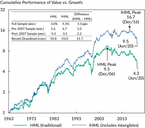
In the full sample, iHML (the factor based on intangibles-adjusted B/P) outperforms the traditional value factor by 1.3 pps per year. We observe a reasonably uniform return advantage averaging about 1 pp per year in the pre-2007 sample. In the post-2007 sample, the performance gap between the B/P-based HML and iHML becomes far more pronounced; at 2.2 pps per year, it chops away two-fifths of the 13½-year loss.

Many low-B/P growth stocks of companies that invest heavily in intangibles are not nearly as expensive after the change to iHML is made. Reciprocally, some value stocks of companies that are disinvesting in their future look surprisingly expensive on this intangibles-adjusted metric, and some even move into the growth portfolio. Once we incorporate intangibles in the book value measure, the drawdown for value shrinks, as Figure 2 reports, by nearly three-fourths in duration, from 13½ years to 3½ years, and by one-fifth in depth—from –54.8% to a (still daunting) –43.0%—with the last new high for value relative to growth occurring in early 2017 instead of early 2007.

The iHML strategy subsumes B/P-based HML, but not vice versa. Appendix B reports that once we for B/P-based HML and other traditional factors, including momentum, the outperformance of the iHML factor relative to B/P-based HML is statistically significant at the 5% significance level.

We emphasize that iHML, like traditional HML, would have performed poorly over the past 3½ years, as reported in the data in Figure 2. Including intangibles does little to insulate the investor against the peril of revaluations: iHML, like its traditional counterpart, suffered from a similar drawdown. In the future, incorporating intangibles in the definition of a B/P-based value factor should help protect the structural value return, however, because a measure that includes intangibles runs a lower risk of misclassifying value stocks as growth stocks, and vice versa.²²

Income Yield, Migration, and Revaluation

Although the popular narratives propose different reasons for why value has underperformed growth, the implications of the narratives can be described by disaggregating value factor relative returns (the performance difference between the value portfolio and the growth portfolio) into three constituent parts: (1) migration, (2) income yield, and (3) changes in value-versus-growth relative valuation, or revaluation.²³ If these elements vary over time—for example, if a structural break permanently alters them—then the returns on value investing will also vary. Using an accounting identity (the decomposition and derivation are detailed in Appendix C), we can attribute the value factor’s return to these three elements as shown in Figure 3. The three elements in the decomposition have the interpretations provided in the following subsections.

Figure 3. The Return to Value from Three Elements

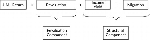
Migration.

The term “migration” is defined as stock-level mean reversion in valuation multiples. It captures the return associated with changes in the composition of the growth and value portfolios. Fama and French (2007) introduced the concept and coined the term “migration” in their study of attribution for the performance of value portfolios relative to growth. They examined stocks’ migration between the six portfolios (small-cap value, neutral, and growth; large-cap value, neutral, and growth) that underlie their HML value factor. They attributed most of the value factor’s performance to the mean reversion in the stocks’ styles. For example, each year some value stocks migrate up into the neutral or growth portfolios and some growth stocks migrate down into the neutral or value portfolios. Both patterns contribute positive performance to value relative to growth—the migration out of value stocks by helping the performance of value portfolios and the migration in by hurting the performance of growth.

Income Yield.

The term “income yield” captures the difference in the change in the book value of equity and dividend yield between the value and growth portfolios. For companies that do not pay any dividends or repurchase or issue shares, this term equals the difference in return on equity (ROE): The change in the book value of equity is equal to retained earnings, and in the absence of dividends, retained earnings are equal to net income. For companies that pay dividends, however, this term slightly understates the difference in ROE because dividends are deflated by the market value of equity rather than the book value of equity. Although this term is close to “profitability,” we call it “income yield” because of this divergence. ²⁴ Growth stocks are typically far more profitable than value stocks while growing faster, which is the reason they deservedly command premium multiples.

Using a discounted-cash-flow model based on subsequent actual performance of a business, which Bill Sharpe termed “clairvoyant value,” and the then-prevailing actual multiples, Arnott, Li, and Sherrerd (2009) demonstrated a roughly 50% cross-sectional correlation between the historical “fair value” multiples of individual stocks. The market appears to be adept at identifying future growth and appears to pay more for that growth than it is worth.

Revaluation.

The term “revaluation” captures the return coming from changes in relative valuations between the growth and value portfolios. Over long periods, unless we allow for a permanent trend in relative valuations (which implies that prices can stray to limitless deviations from fundamentals), these changes in valuations should not contribute significantly to a factor’s performance.²⁵

We will show later that revaluation explains two-thirds of the annual variance in the HML factor’s performance. Fama and French (2002) and Arnott and Bernstein (2002) showed that the equity risk premium can significantly benefit or lose from changes in valuations, even when the premiums are measured over many decades. They argued that the returns induced by the changes in the valuations should be purged from the estimates of the risk premium because no a priori reason exists to explain why any trend in valuation should persist. Following Arnott, Beck, Kalesnik, and West (2016), we extend this argument to the value factor premium.

The Value Factor Premium.

The migration and income yield components are at the core of the value premium. Combined, they form what we call “the structural component” of the value premium. A reasonable expectation is that income yield and migration will persist, with income yield always benefiting growth stock returns, migration always benefiting value, and revaluation following something of perhaps a mean-reverting random walk. Accordingly, we describe the first two as structural sources of return. Because the changes in aggregate valuations cannot trend indefinitely—which is equivalent to saying that no bubble can last forever—the revaluation component should average roughly zero over a sufficiently long period. That said, relative valuations of value and growth stocks could drift to a “new normal,” and the value factor would, as a result, earn an abnormal (good or bad) return during the transition period.

Table 3 displays the results of the value factor’s return decomposition in the pre- and post-2007 samples; the attribution details are available in Appendix C. (We provide details of the attribution for the six HML portfolios in Appendix D found in the supplemental online material.) Because our value strategy (HML) was rebalanced annually at the end of June and because our decomposition used the observations between rebalancing points, our analysis focuses on the periods between rebalancing points. Specifically, for the pre-2007 period, we examined the period from July 1963 through June 2007, and for the post-2007 period, we examined the period from July 2007 through June 2020.

Table 3. Attribution of Value Factor Returns

Size	Valuation	Total Return (%)	Revaluation Premium (pps)	Structural Premium (pps)	Income Yield (pps)	Migration (pps)
A. Return decomposition, July 1963–June 2007
Small	Value – growth	8.4	0.1	8.3	–17.7	26.0
Big	Value – growth	3.8	0.3	3.5	–8.8	12.4
Average	HML	6.1	0.2	5.9	–13.2	19.2
B. Return decomposition, July 2007–June 2020
Small	Value – growth	–4.8	–4.9	0.2	–23.1	23.3
Big	Value – growth	–7.5	–9.6	2.0	–8.8	10.8
Average	HML	–6.1	–7.2	1.1	–15.9	17.0
C. Full-span return decomposition, July 1963–June 2020
Small	Value – growth	5.4	–1.1	6.5	–18.9	25.4
Big	Value – growth	1.2	–2.0	3.2	–8.8	12.0
Average	HML	3.3	–1.5	4.8	–13.9	18.7

Note: Log returns used in the attribution (see Appendix C).

Sources: Research Affiliates, LLC, using data from CRSP/Compustat.

On average, because growth stocks were more profitable and faster growing than value stocks, the income yield difference contributed –13.2 pps per year to the value-minus-growth return in the pre-2007 period. Over the same period, the migration component, at 19.2 pps a year, more than offset the difference in income yield. Combining the income yield and migration components, we observe a structural value return of 5.9% per year, which is near the average HML premium return of 6.1%. Revaluation played only a small role in this 44-year span.

In the post-2007 sample shown in Table 3, the income yield and migration components are close to their values in the pre-2007 sample. The income yield differential widened, however, suggesting that today’s growth stocks are in some ways better businesses than the growth stocks of the past, although not by much. Meanwhile, the migration effect narrowed. ²⁶ So, migration seems to have slowed, as valuation spreads have widened, although again, not by much. Their sum—the structural return—is distinctly smaller than before 2007, but it remains positive and economically meaningful. The value effect appears to be alive and well, albeit weaker than in the past.

As Table 3 shows, revaluation in the post-2007 sample contributed –7.2 pps annually to the return, down from an average upward contribution of 0.2 pp before 2007. As a result, the total value return has flipped from 6.1% in the first 44 years to an annualized shortfall averaging –6.1% in the past 13 years. It took value cheapening relative to growth by 7.2 pps per year to create a performance shortfall of 6.1% per year. Since 2007, well more than 100% (116%) of the shortfall of value relative to growth is a consequence of value becoming cheaper relative to growth. In the most recent 13-year period, the revaluation component appears to be the key to understanding why growth stocks are outperforming value stocks.

Figure 4 illustrates the evolution of the cumulative value return (left axis), which is the same as in Figure 2, and the value–growth relative valuation (right axis).

Figure 4. HML Value Factor Performance and Relative Valuations: US Market, July 1963–June 2020

Notes: We computed the relative valuations each month by constructing a monthly rebalanced version of HML. The signal is the book value of equity from a fiscal year that ended at least six months earlier divided by the market value of equity lagged by six months. This signal matches the signal of the annually rebalanced HML: When HML was rebalanced at the end of June in year t, the book value of equity is from the fiscal year that ended in year t – 1 and the market value is from December of year t – 1. Our monthly version of HML matches the standard HML’s valuations at the rebalancing points while still tracing out valuations at a monthly frequency. Moreover, because most US companies have December fiscal year-ends, the value factor (HML) becomes predictably cheaper at the June rebalancing date. This rebalancing effect then dissipates over the following year. We removed the resulting seasonalities from valuations by subtracting the calendar month–specific (e.g., February) mean valuation and adding back the unconditional mean valuation. An alternative method for constructing a timely measure of value (and valuations) is the “HML devil,” which divides the lagged book value of equity by the current price (Asness and Frazzini 2013). The $r^{HML}$ is HML return, and $\Delta p{b}_t$ is the change in the logarithm of the price-to-book ratio.

Sources: Research Affiliates, LLC, using data from CRSP/Compustat.

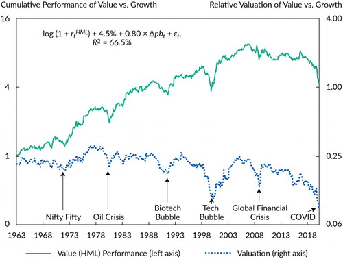
The relative valuation is the ratio of B/P for the growth portfolio to B/P for the value portfolio. If the B/P of the growth portfolio is 0.4 and the B/P of the value portfolio is 2, then the relative valuation is 0.20. The median relative valuation is 0.21, which means that (when measured by B/P) growth stocks have been, on average, about 4.8 times more expensive than value stocks.²⁷ As Figure 4 shows, however, the valuations of value stocks, measured relative to growth, have fluctuated widely over time and correlate strongly with the concurrent performance of the value factor.

When we put the performance and the revaluation charts together, the short-term movements of the two appear to be joined at the hip. In the short run, the revaluation component (changes in the B/P of value relative to growth) is the dominant driver of the value portfolio’s performance relative to growth. Over the long run, however, the two lines diverge. This wedge of divergence suggests that the value premium is driven by structural return and is not a lucky discovery because of a temporary revaluation. Indeed, the factor has delivered impressive long-term profits, despite a substantial downtrend in relative valuations. The regression reported in Figure 4 shows that log changes in valuations explain two-thirds of the variation in the log HML returns.

We observe what seems to be a pronounced trend that may reflect the waning relevance of classically defined book value as a valuation metric. Nevertheless, even a substantial trend over the past 57 years amounts to only a 0.8% negative annualized slope, ²⁸ and the valuation spreads may be abnormally high at the start of the series and/or abnormally low at the end.

The relative valuation in 1963 is at the time-series median of 0.21. The relative valuation varies from 0.30, five years after the Nifty Fifty bubble burst, to 0.10, at the peak of the dot-com bubble, to 0.085 at the end of June 2020. In every episode when value substantially underperformed growth, a key driver was value stocks’ becoming cheaper relative to growth stocks.

During the drawdown from 2007 to 2020, the value factor lost a cumulative 54.8% in performance, or –6.2% per year. From July 2007 to June 2020, the relative valuation moved from 0.23, which is relatively expensive at the 25th percentile of the distribution, to 0.085, at the cheapest relative valuation percentile ever. One way to view this comparison is that it took a 64 pp drop in relative valuation, value relative to growth, to create a 55% drawdown.²⁹

At the current valuation level, growth stocks trade nearly 12 times the P/B valuations of value stocks. The relative valuation has been close to this level only twice over the 57-year history of our analysis: the peak of the dot-com bubble and the nadir of the global financial crisis. Our decomposition indicates that the change in relative valuation since mid-2007 contributed –7.2 pps per year and turned the 1.1% structural return into the –6.1% per year realized value return.

Alternative Definitions of Value

The B/P HML has performed the worst of any of the other definitions analysts use—and over a longer span. Every measure of value that we considered, however, has underperformed, and the bulk of that underperformance has been associated with a large drop in relative valuations. This behavior is not limited to the B/P-based HML. Table 4 displays the performance characteristics of five segments of the B/P-based HML value metric and four alternative value strategies. Unlike our other tables, we used arithmetic returns instead of log returns in our analysis. We constructed each of the four alternative value strategies, including iHML, described in the previous section, by using the Fama–French methodology for constructing the growth, neutral, and value portfolios. ³⁰ We also show results for a composite of the equally weighted relative B/P, the earnings-to-price ratio (E/P), the sales-to-price ratio (S/P), and the dividend yield for stocks that paid dividends.³¹

Table 4. Performance of Alternative Value Definitions: US Stocks

	July 1963–December 2006		January 2007–June 2020		July 1963–June 2020		Historical Percentile Rank		Raw Percentile Rank
Value Definition	Average	t-Stat.	Average	t-Stat.	Average	t-Stat.	June 2007	June 2020	June 2007	June 2020
HML (book to price)	5.6%	3.86	–5.4%	–2.00	3.0%	2.34	32%	100%	32%	100%
HML, small cap	7.5	4.33	–4.5	–1.69	4.6	3.14	60	100	63	100
HML, large cap	3.8	2.47	–6.2	–1.92	1.4	1.02	15	100	14	100
Value to neutral	2.4	3.40	–1.9	–1.06	1.3	1.98	54	98	52	98
Neutral to growth	3.3	2.73	–3.5	–2.38	1.7	1.71	14	100	14	100
iHML, ibook to price	6.7	5.17	–3.2	–1.27	4.3	3.73	5	100	3	100
E/P	5.2	3.08	–2.2	–0.93	3.5	2.46	39	88	37	91
S/P	5.8	4.01	–1.0	–0.51	4.2	3.46	25	98	25	98
Composite	4.9	2.87	–3.6	–1.34	2.9	1.98	44	95	43	95

Notes: In the value-to-neutral and neutral-to-growth definitions, neutral refers to the middle 40% of stocks by B/P. Recall that value comprises the 30% of stocks with the highest B/Ps and growth comprises the 30% of stocks with the lowest B/Ps. For the portfolios defined by intangibles-adjusted iHML, by the E/P, and by the S/P, we followed the HML convention: groups of 30% value, 40% neutral, and 30% growth. Each of the large-cap and small-cap universes were equally weighted by the respective large-cap or small-cap results for each of the value, growth, and neutral portfolios. We averaged earnings, sales, or dividends over the previous five years so that the portfolio definitions would be insensitive to cyclical peaks and troughs, following Arnott, Hsu, and Moore (2005). For the rightmost columns of percentile ranks, we measured the valuation percentiles in June 2007 and June 2020 by using the same ratio used to form the portfolios.

Sources: Research Affiliates, LLC, using data from CRSP/Compustat.

As Table 4 shows, when all four alternative value factor definitions were used, we found that value underperformed growth in the post-2007 period. Also, for all the definitions, value’s underperformance was associated with value having neutral-to-expensive relative valuations in June 2007 and having bottom-decile relative valuations in June 2020. Interestingly, the large-cap half of the HML factor experienced the largest underperformance, –6.2% per year, in the post-2007 period, which was accompanied by a huge move in relative valuations from the 15th percentile to the cheapest percentile.

The value-to-neutral and neutral-to-growth factors have similar underperformance (and combined, match the HML underperformance), so the results are symmetrical. The value-to-neutral factor is long the 30% of stocks with the highest B/Ps and short the 40% of stocks in the middle of the B/P distribution. The neutral-to-growth factor is long the neutral stocks and short the 30% of stocks with the lowest B/Ps. The valuation change for the neutral-to-growth definition nearly matches the move for large-cap HML from the 15th percentile, well into the top quintile, to the cheapest percentile. The ending percentile implies that the growth portfolio trades today at unprecedented valuations relative to neutral, not only relative to value.

The traditional B/P-based HML strategy suffered the worst drawdown, underperforming by –5.4% per year,³² whereas the five alternative strategies, reported in the bottom half of Table 4, fared much better. The iHML strategy cut that shortfall in half, but even the adjustment of book value to include intangibles did not fare as well as the E/P or S/P value factor models after 2007. The underperformance from January 2007 through June 2020 ranges from –1.0% per year for the S/P-based value factor to –3.6% per year for the composite, which was clearly hurt by including traditional HML in its process.

We emphasize that the B/P-based HML model is the worst model in this comparison after 2007. Losses from the other value metrics range from modest for S/P to moderate for iHML and the composite. Not shown in Table 4 is that every metric other than HML has seen a drawdown ranging from 3½ years to 6½ years since the previous peak; also not shown is the grinding 13½-year dry spell for HML.

What to Expect from Value?

In the aftermath of the tech bubble in 2000, the relative valuation of B/P-based HML rose from what was then a record low of 0.10 in June 2000 to a borderline top-quartile valuation of 0.25 in June 2005, delivering 110% return for value relative to growth in just five years. Then, value stalled. Over the past 13½ years, the relative valuation of HML (value versus growth) moved from the top quartile (specifically, the 25th percentile) to a new record low in relative valuation and a newly reset 100th (lowest) percentile.³³ We display the historical probability density of relative valuations in Figure 5. This downward revaluation since 2007 explains more than 100% of value’s underperformance and two-thirds of its annual variability. Today, the relative valuation of the HML value factor is in its most attractive valuation percentile in history, considerably cheaper than the relative valuation of value stocks at the peak of the tech bubble in 2000.

Figure 5. Historical Distribution of Relative HML Valuations: US Market, July 1963–June 2020

Notes: We estimated the theoretical distribution of valuations using kernel density estimation. We took the realized distribution of valuations from Figure 5 and used the Epanechnikov (parabolic) kernel with optimal bandwidth. This method can be considered to fit a smooth “density” over the historical histogram of valuations; it fills the gaps and makes educated guesses about the distribution outside the highest and lowest historical valuations. We have also placed the July 2007 and June 2020 relative valuations in this distribution plot.

Sources: Research Affiliates, LLC, using data from CRSP/Compustat.

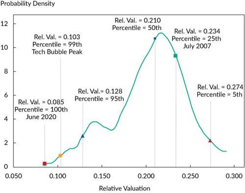
Figure 5 illustrates that most of the historical observations of relative valuations (about 70%) are concentrated between the values of 0.17 and 0.25 (and 90% are between the values of 0.13 and 0.27). Outside the 70% range, the historical observations have quite fat tails in both directions.

Given the historical relationship between value’s starting valuation levels and value’s subsequent return, what return can we reasonably anticipate from the expected value premium in the years ahead? Should we expect a sharp rebound in value, as we observed after the tech bubble of 1999–2000, the global financial crisis, and the Nifty Fifty bubble of 1972–1973? We can gauge the forward-looking expected return estimates of the value premium by using the decomposition into revaluation, migration, and income yield of Table 3.

We cannot, of course, simply assume a revaluation return to the historical median and keep the other components at their historical averages. Over the 1963–2020 period, the correlation between the income yield and revaluation terms is –0.32, between the income yield and migration terms is –0.43, and between the revaluation and migration terms is –0.04.³⁴ These negative correlations mean that when the HML factor benefits from a tailwind of upward revaluation, the lower income yield and migration terms typically offset some of the revaluation profits.

The question we want to answer is, What is the expected return on HML conditional on any given magnitude of revaluation? Conveniently, if we use historical data as a guide and model the conditional expected returns, we can use linear regression to provide some answers.

What HML return can we expect in a year when a specific scenario is realized? Table 5 displays the estimates. ³⁵ The central assumption of our analysis is that revaluations will not exhibit a permanent trend (otherwise, prices would be indefinitely unmoored from fundamentals). Even if the relative valuations were to stay at the current level, value investors should still expect to collect the structural return of 4.5% as estimated over the full 57-year sample (see Figure 4).³⁶ Because of the presence of structural return, a further decline over the next year from the current bottom-percentile valuation to yet another new low, at a relative valuation of 0.081 or lower, would be required for value to have a zero or negative return.

Table 5. Scenario Analysis: Forward-Looking Expected Return, Conditional on Revaluation

Directional Change	Scenario End Point	Relative Valuation	Log Relative Valuation Z-Score	Historical Percentile Rank	Return
Expanding relative valuations	Negative 6-σ deviation	0.061	–6.00	Beyond 100th	–21.8%
	Negative 5-σ deviation	0.075	–5.00	Beyond 100th	–5.3
	Zero premium	0.081	–4.68	Beyond 100th	0.0
No change	Stay at 100th percentile	0.085	–4.40	100th	4.5
Contracting relative valuations	Move to 95th percentile	0.128	–2.43	95th	37.1
	Move to 90th percentile	0.143	–1.90	90th	45.8
	Move to 75th percentile	0.181	–0.75	75th	64.8
	Move to 50th percentile	0.211	–0.02	50th	76.8
	Halfway mean reversion	0.134	–2.20	93th	40.8
Starting levels		0.085	–4.40	100th

Notes: For projections, we used a regression-based model that captures the relationship between year-over-year changes in relative valuations and contemporaneous returns. The model accounts for the potential cross-correlation between terms and was calibrated over the full sample of July 1963–June 2020. Shown are the regression results in Figure 3. Implied returns were trivially computed from this linear model once we knew the starting and ending points in the relative valuations. Similarly, we used the model to compute the level of changes in relative valuations required to generate a zero HML return in the first row of the table. We computed the halfway mean-reversion point by using the regression of the B/P-relative HML valuation against the year-earlier valuation.

Sources: Research Affiliates, LLC, using data from CRSP/Compustat.

Historically, relative HML and iHML valuations have shown a tendency to revert to the mean. A regression of the B/P-relative HML valuation against the year-earlier valuation has an intercept of –0.41 (t-statistic = –2.55) and a slope of 0.73 (t-statistic = 6.84). The slope roughly corresponds to a rapid 2.2-year half-life mean-reversion rate. ³⁷ The negative intercept reflects the trend in the relative valuations, which is not surprising given the extreme end-point valuation. Although the trend in the period that we examined is statistically different from zero, in the very long run it should be, in the absence of Ponzi schemes and perpetual erosion in the comparability of different companies’ book values, zero. These estimates are average historical tendencies, which never play out exactly.

Full reversion to the median, if it happened in a single year, would require value to beat growth by 77% (on a log scale, meaning that value would more than double relative to growth). If this were to happen over several years instead of a single year, the structural return of the value factor would add to this return every year, generating an even larger gain (although a lower annualized gain). Even a move to the historical 75th percentile, halfway between cheapest-ever and the median valuation for value relative to growth, should deliver 65% relative performance for value over growth. Arguably the most surprising result in Table 5 is that a modest improvement from the current 100th percentile to the 95th percentile—the midpoint of the cheapest decile in history—would result in a return of about 37%. Finally, even if valuations were to stay at current levels, the model suggests a positive 4.5% return, driven solely by the average structural return of the past 57 years. Of course, we have no guarantee that the relative valuation will not continue its recent trend, thereby moving beyond the current 100th percentile. For example, a move to a level corresponding to a 5-σ deviation should result in a –5.3% return, and a move to a 6-σ deviation should result in a –21.8% return.

No one knows with certainty whether we will return to the lofty structural return earned through 2006, whether mean reversion in relative valuation will happen, how long the mean reversion will take, or if the mean has itself shifted to a new normal, perhaps because of the increasing importance of intangibles. From the peak of the tech bubble in early 2000 to the peak for value stocks in early 2007, HML appreciated from the then-cheapest percentile ever to the 25th percentile—marginally top quartile—in just seven years. Recoveries following the Nifty Fifty bubble and the global financial crisis both happened more rapidly. The present and future rarely play out in the same way as the past. We have our expectations, but others can and will set their own.

Conclusion

Many narratives purport to explain why “this time is different,” why value may be structurally impaired. These narratives include (among others) the new-normal interest rate environment, the growth of private markets, crowding, decreased migration, stranded assets, and technological change. We examined many of these explanations and found insufficient evidence to declare a structural break.

We addressed the important issue of mismeasurement of value because of a core failing of book value as a valuation metric. This classic measure of value was designed at a time when the economy was much less reliant on intellectual property and other intangibles. In today’s economy, intangible investments play a crucial role, especially in growth stocks and even in value stocks, yet book value ignores most internally sourced (intangible) investments. We capitalize intangibles and show that this measure of value outperforms the traditional measure, notably beating B/P-based HML by nearly a twofold margin after 1990. Nonetheless, this improved measure of value has also recently suffered a large drawdown and after 2007 has still not been as good as S/P or E/P. Perhaps intangibles-adjusted B/P is still missing something important.

We also offered a simple model that decomposes the returns of value relative to growth. The framework attributes the relative performance to three components: migration, income yield, and change in relative valuation. Our evidence suggests that the sum of migration (e.g., individual value stocks becoming growth stocks) and income yield is marginally smaller, albeit not materially different, in the post-2007 period than it was in the pre-2007 period. ³⁸ Migration benefits value stocks and income yield benefits growth stocks; with migration reliably dominating income yield, the result is the value premium. We refer to the combination of the two as the “structural return.”

The fact that B/P HML has suffered a –55% drawdown has nothing to do with failings in the structural return and is entirely the result of the collapse of relative valuations. Over the drawdown period, relative valuations have moved from the 25th to the 100th percentile, with value stocks becoming cheaper relative to the market while growth stocks have soared. Oversampling a period of negative residuals may also have contributed modestly to the drawdown. Our initial bootstrap analysis, which did not account for changes in valuations, suggests that the current drawdown would have been thought to be 2.3% probable. This is true despite relying on past returns that excluded the current drawdown period—that is, based on historical data from 1963 through mid-2007, a span in which value beat growth by 6% per year. We believe this outcome is improbable, but it is not an extreme outlier.

As of mid-2020, valuations for value relative to growth are in the extreme left tail of the historical distribution. If, as history suggests, there is any tendency for mean reversion, the expected future returns for value, by almost any definition, should be above historical norms. Indeed, we showed that, even if the relative valuation remains in the current bottom percentile, the structural components (migration and income yield) should offer a positive overall return.

Nevertheless, we would like to emphasize two important caveats. First, the percentiles are backward looking; it is possible to cross, yet again, into unexplored territory. Second, returns are noisy. Although expected returns of value relative to growth are high, the role of luck (both good and bad) creates a wide distribution of outcomes over short spans, even over the next five years. Although value strategies seem as attractive as they have ever been—that is, they are highly likely to outperform—an elevated expected return is not a guarantee that value must outperform growth in the years ahead.

Acknowledgments

We appreciate the comments of Stephen J. Brown (executive editor), Magnus Dahlquist, Sina Ehsani, and Alex Pickard. Kay Jaitly, CFA, and Jaynee Dudley provided editorial assistance.

Notes

¹ Appendix A provides a histogram of the worst drawdowns from June 1963 through June 2020.

² For our purposes, except as otherwise noted, we define relative valuation as the ratio of the B/P for the growth portfolio measured relative to the B/P for the value portfolio. In the case of the standard B/P-based value factor, we measure the B/P of the growth portfolio relative to the B/P of the value portfolio.

³ Arnott, Kalesnik, and Wu (2017) and Patton and Weller (2020) complemented the analysis in Lettau et al. (2019). They found that those funds with value exposure earn only a fraction of the value premium after accounting for implementation costs.

⁴ The FANMAG stocks combine the so-called FANG stocks (Facebook, Amazon, Netflix, and Google) with the largest survivors from the tech bubble of 20 years ago, Apple and Microsoft. Apart from Saudi Aramco, which has less than 2% of its shares held by the public, the five most valuable companies in the world, three with a market value greater than US$1 trillion, were on the FANMAG list as of midyear 2020.

⁵ In the standard HML definition of the value factor, this rebalancing happens annually at midyear. This rebalancing effect—value becoming cheaper and growth more expensive with each rebalance—means that the valuation of the value portfolio relative to growth becomes materially cheaper every time the portfolios are rebalanced and then moves the other way over the next 11 months. To adjust for this effect in our tests, we rebalanced HML monthly rather than annually and then removed any remaining seasonalities (which emanate from most companies’ fiscal years ending in December) by computing seasonally adjusted revaluation metrics.

⁶ Indeed, most multifactor strategies now trade at premium valuation multiples relative to the market, so even those who claim to embrace value as a key part of their strategy are now allowing growth to swamp value in their portfolios.

⁷ For example, Barbee, Mukherji, and Raines (1996) documented the value effect for the price-to-sales ratio; Stattman (1980) and Rosenberg, Reid, and Lanstein (1985) documented the value effect for B/P; and Naranjo, Nimalendran, and Ryngaert (1998) showed the value effect for the dividend yield. Jacobs and Levy (1988) demonstrated that many different definitions of value are related and that they produce correlated returns.

⁸ The equal weighting of small- and large-cap stocks introduces a weighting peculiarity in which the largest-cap stocks in small-cap value and small-cap growth portfolios receive a weighting more than 10 times that of the smallest-cap names in the large-cap value and large-cap growth portfolios.

⁹ Importantly, as Table 1 illustrates, value is not the only factor with disappointing recent performance, albeit other factors’ travails are of a lesser magnitude. As Arnott, Harvey, Kalesnik, and Linnainmaa (2019) pointed out, the likely drivers for the recent disappointing factor performance include (1) exaggerated expectations for the long-term factor premiums because of data mining, (2) factors being far riskier than investors perceive because of high potential skewness and kurtosis, and (3) overstated benefits of diversification.

¹⁰ Unless otherwise noted, our return measures are log returns when we are discussing long-term compound rates of return and are simple returns when we are examining individual samples or, as in this case, a cumulative return.

¹¹ Davis, Fama, and French (2000) analyzed HML performance back to 1926 and found that its average return from July 1929 through June 1963 was 0.50% per month. In this pre-1963 sample, value’s worst drawdown is –43.5%, which was reached at the end of March 1935.

¹² Harvey, Liu, and Zhu (2016) studied the overfitting issue and declared the HML version of value “significant” after controlling for test multiplicity as of 1992.

¹³ According to the Bloomberg Barclays Global Aggregate Negative Yielding Debt Index.

¹⁴ As of 30 June 2020, 3,622 companies were publicly traded on the NYSE, AMEX, and NASDAQ.

¹⁵ Specifically, Graham and Dodd (1934, p. 17) wrote (emphasis added), “In general terms [intrinsic value] is understood to be that value which is justified by the facts, e.g., the assets, earnings, dividends, definite prospects, as distinct, let us say, from market quotations established by manipulation or distorted by psychological excesses. But it is a great mistake to imagine that intrinsic value is as definite and as determinable as is the market price. Some time ago intrinsic value (in the case of common stock) was thought to be the same as ‘book value,’ i.e., it was equal to the net assets of the business, fairly priced. This view of intrinsic value was quite definite, but it proved almost worthless as a practical matter because neither the average earnings nor the average market price evinced any tendency to be governed by book value.”

¹⁶ The alternative system to GAAP, International Financial Reporting Standards (IFRS), similarly undercapitalizes the intangible expenses, but the two systems have a noticeable difference. IFRS allow for a partial capitalization of internally incurred development costs (but not research or other types of intangibles-related expenses).

¹⁷ The two main components of the book value of equity are contributed capital and retained earnings (Ball, Gerakos, Linnainmaa, and Nikolaev 2020). Contributed capital represents the net contribution of capital from the company’s shareholders through initial or seasoned public offerings in excess of share repurchases. Retained earnings are the earnings accumulated since the company’s inception minus accumulated dividends. Beneish, Harvey, Tseng, and Vorst (forthcoming) studied how intangible capital is incorporated into book value in mergers and acquisitions.

¹⁸ Following Peters and Taylor (2017), we would capitalize R&D expenses by applying the perpetual inventory method to the company’s past R&D: $G_{i,t}=\left(1-\delta \right)G_{i,t-1}+{\text{R\&D}}_{i,t}$, where $G_{i,t}$ is the end-of-period stock of knowledge capital for company i, $\delta$ is the industry-specific discount rate, and ${\text{R\&D}}_{i,t}$ is the real company R&D expenditures during the year. We thank Ryan Peters and Lucian Taylor for providing the company-level estimates of intangible capital. We apply the estimated discount rates from the Bureau of Economic Analysis for R&D for different industries. Examples of R&D expenses include patents, software, and internal knowledge development costs. The R&D capitalized measure could be interpreted as the replacement cost of the knowledge capital. Similarly, we capitalize 30% of SG&A expenses by using a depreciation rate of 20% for all industries. Just as with R&D, the capitalized SG&A expense could be interpreted as the replacement cost for creating brand awareness, training costs to build human capital, and so forth. The perpetual inventory method requires assumptions about the initial stocks of knowledge (R&D) and organization (SG&A) capital at the time of the IPO. Following Peters and Taylor (Appendix B), we constructed these initial stocks by using average pre-IPO growth rates.

¹⁹ It is arbitrary to capitalize 100% of R&D and 30% of SG&A expenditures and no less arbitrary to choose any particular amortization rules. It will be an interesting topic for future research to gauge which metrics perform best in producing a better HML value factor or in predicting future corporate profits and whether optimal settings for these metrics vary by industry, sector, or country. We found it a striking result that our first crude effort to introduce intangibles into book value led to a 50% improvement in the efficacy of HML over the past 40 years and a near doubling of its efficacy over the past 30 years.

²⁰ Following Fama and French (1993), we constructed six portfolios by sorting stocks by size (providing small and big groups) and by book value to market value (providing growth, neutral, and value segments). The value portfolio in Figure 1 is the average of the ratios of the small/value and big/value portfolios, and the growth portfolio is the average of the small/growth and big/growth portfolios.

²¹ Li (2020) and Park (forthcoming) also constructed iHML factors that incorporate intangibles. Also, see Lev and Srivastava (2019).

²² When we incorporate intangibles into book value, the labels “growth” and “value” become even more inappropriate than they already are. A “cash cow” company, spending nothing on intangibles, may pop into the growth portfolio merely because its book to price is newly lower relative to other companies, which does not mean the company is pursuing growth, only that it is expensive.

²³ The idea of decomposing the return of equity factors into structural and revaluation components was first introduced by Arnott, Beck, Kalesnik, and West (2016).

²⁴ Cohen, Polk, and Vuolteenaho (2003) showed that about half of the information contained in the B/P differences between value and growth stocks is attributable to the differences in their future profitability, which is highly correlated with the differences in income yield in our decomposition. They found that persistence in growth stocks’ valuations reflects their future expected (15-year) profitability, which tends to support their trading more expensively than value stocks.

²⁵ We assume that valuations do not exhibit endless bubbles, a more relaxed assumption than the one by Cohen et al. (2003) or Asness, Friedman, Krail, and Liew (2000) that relative valuations revert to the mean. The mean-reversion assumption would further strengthen the argument.

²⁶ This narrowing is consistent with the finding of Lev and Srivastava (2019) that migration has slowed. Our decomposition puts a number on how much this slowdown has lowered the returns on value investing: 2.2 pps per year.

²⁷ We report summary statistics for relative valuation, such as the median and values at specific percentiles, by using the monthly observations of relative valuations.

²⁸ We obtained the slope by regressing the log valuation ratio on the annualized time trend. We interpret the slope to mean that the valuation, on average, has been declining by about 0.8% per year over the 57-year sample.

²⁹ If a stock falls 55% and its P/B falls by 64%, we can choose to react emotionally (“Get me out of here!”) or in a contrarian fashion (“I can’t believe how cheap this is!”) or somewhere in between. We lean toward the contrarian reaction, but we could of course be wrong!

³⁰ Again, in keeping with the Fama–French methodology, we did this exercise for both large- and small-cap stocks and then equally weighted the resulting large and small growth, value, and neutral portfolios.

³¹ We do not separately show results for dividend yield because most of the “action” in growth stocks—for more than a quarter-century—has been in companies that paid no dividends. Excluding those stocks made no sense.

³² This amount differs from the –6.1% in Table 3 because these results reflect arithmetic returns rather than log returns and a slightly different time span, one beginning in January 2007 instead of July 2007.

³³ The relative valuation of iHML moved from the 40th percentile to the 98th percentile over the same 13½-year period. The similarity in the movements in the relative valuations of HML and iHML suggests that the omission of intangible capital from the classical definition of value does not explain why value has become exceedingly cheap relative to growth since 2007.

³⁴ Based on unreported results that are available on request.

³⁵ In the scenario analysis shown in Table 5, we considered movements in an estimated theoretical distribution of relative valuations. We provide additional details in Appendix E, found in the supplemental online material.

³⁶ We estimated the forecasting model’s parameters from the entire sample period. Because the model is linear, the projections could be adjusted for alternative assumptions about the structural alpha by adding (or subtracting) the difference versus an alternative assumed level.

³⁷ A slope less than 1.0 would be associated with mean reversion, a slope greater than 1.0 would be associated with momentum, and a slope not significantly different from 1.0 would imply no autocorrelation.

³⁸ In Appendix E in the supplemental online material, we provide analysis demonstrating that the apparent reduction in the structural premium is largely explained by the left-tail hypothesis. We do not have significant evidence for a structural break.

Appendix A.

Histogram of Largest Drawdowns

In Figure A1, we display the distribution of the largest drawdowns in the simulations. Each bar in the histogram shows how common a worst drawdown of the indicated magnitude is.

Figure A1. Histogram of Largest Drawdowns for HML Value Factor Based on 1 Million Simulations

Note: Bootstrap simulations are drawn from US HML returns for July 1963–December 2006.

Sources: Research Affiliates, LLC, using CRSP/Compustat data.

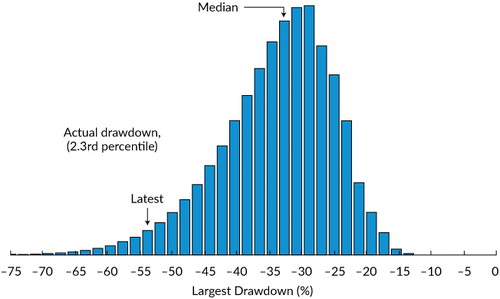
Appendix B.

iHML vs. HML Spanning Tests

Table B1 reports the results of spanning tests of HML and iHML. These regressions measure the extent to which HML or iHML subsume (i.e., “span”) each other when one also controls for the market, size, and momentum factors. With conventional B/P, the coefficients for market (beta) and size are negative, which suggests that value has a low-beta and large-cap bias on average over time. With iHML, incorporating intangibles, the signs flip and the coefficients become slightly more neutral, suggesting that iHML value has a mild high-beta and small-cap bias.

Table B1. HML vs. iHML Spanning Tests: US Market, July 1963–June 2020 (t-statistics in parentheses)

	Dependent Variable: HML				Dependent Variable: iHML
	(1)	(2)	(3)		(4)	(5)	(6)
Alpha, annual	3.04*	3.97**	–0.19		4.34**	4.57**	1.34**
	(2.34)	(3.12)	(–0.36)		(3.73)	(3.90)	(2.64)
Market		–0.14**	–0.07**			–0.04	0.04**
		(–6.11)	(–6.73)			(–1.63)	(3.57)
Size			–0.21**				0.20**
			(–13.99)				(13.82)
Momentum			–0.02				–0.02
			(–1.56)				(–1.82)
Value (HML)							0.81**
							(53.74)
Value (iHML)			0.99**
			(56.26)
N	684	684	684		684	684	684
Adjusted R^2		5.0%	84.4%			0.2%	82.4%

Notes: Column numbers identify the individual models in the spanning tests. In columns 1–3, traditional HML was regressed on the market, size, and momentum factors (following Carhart 1997) as well as on iHML. Standard errors are clustered at the company level. Significance is measured under the assumption of a single hypothesis test.

* Significant at the 5% level.

** Significant at the 1% level.

Sources: Research Affiliates, LLC, using data from CRSP/Compustat.

When iHML is included, the alpha is negative and not statistically significantly different from zero, implying that iHML completely subsumes HML. In columns 4–6, iHML is the dependent variable and is regressed on the market, size, and momentum factors, as well as on the traditional HML factor. In this case, the alpha for iHML is significant at the 5% level under the assumption of a single hypothesis test. This result is consistent with iHML subsuming HML but not the opposite.

Appendix C.

Return Decomposition Details

In the section “Income Yield, Migration, and Revaluation,” we describe a decomposition of a portfolio’s return into three parts: the revaluation, income yield, and migration components. Here, we derive this decomposition by starting from the definition of log returns. We then show the decomposition results for the value and growth portfolios’ log returns as well as for the log HML return. The revaluation term captures the return coming from the change in relative valuations. The income yield term captures the retained earnings (reflected as the change to the book value of the company) and the dividend distribution. The migration term captures the return resulting from changes in valuations net of the revaluation. The decomposition we derived holds as an identity for the portfolios’ log returns. In Table 3, in which we show the decomposition of the HML factor’s return (not the log return), the decomposition holds as an approximation. The decomposition uses the following notation:

$r_{t^{+}}$ = return from time t − 1 to time t on the portfolio formed at time t − 1

$D_{t^{-}}$ = dividend distributions from time t − 1 to time t from the portfolio formed at time t − 1

$P_{t-1}$ = portfolio-weighted market capitalization at time t − 1 of the portfolio formed at time t − 1

$B_{t-1 }$ = portfolio-weighted book value of equity at time t − 1 for the portfolio formed at time t − 1

$B_{t^{-}}$ = portfolio-weighted book value of equity at time t for the portfolio formed at time t − 1

$P_{t^{-}}$ = portfolio-weighted market capitalization at time t of the portfolio formed at time t − 1

$P_{t^{+}}$ = portfolio-weighted market capitalization at time t of the portfolio formed at time t

$B_{t^{+}}$ = portfolio-weighted book value of equity at time t of the portfolio formed at time t

With this notation, a return on a portfolio can be represented as shown in Figure C1.

Figure C1. The Return to Value from Three Elements: Detailed Examination

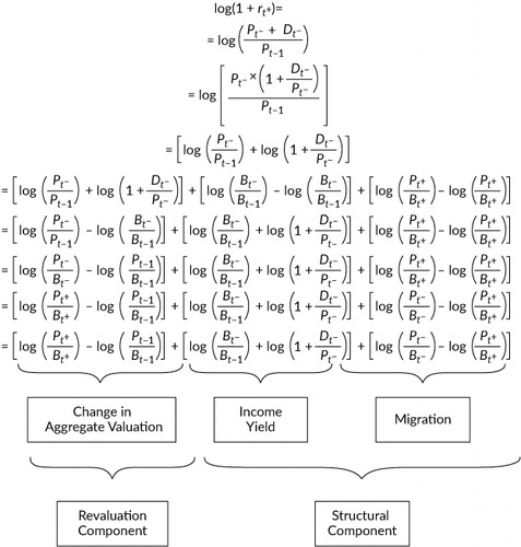
This decomposition holds as an identity for a portfolio’s log returns.

References

- Arnott, Rob, Noah Beck, Vitali Kalesnik, and John West. 2016. “How Can ‘Smart Beta’ Go Horribly Wrong?” Research Affiliates article (February) https://doi.org/10.2139/ssrn.3040949.
- Arnott, Robert, and Peter Bernstein. 2002. “What Risk Premium Is ‘Normal’?” Financial Analysts Journal, vol. 58, no. 2: 64–85 https://doi.org/10.2469/faj.v58.n2.2524.
- Arnott, Rob, Campbell R. Harvey, Vitali Kalesnik, and Juhani Linnainmaa. 2019. “Alice’s Adventures in Factorland: Three Blunders That Plague Factor Investing.” Journal of Portfolio Management, vol. 45, no. 4: 18–36 https://doi.org/10.3905/jpm.2019.45.4.018.
- Arnott, Rob, Campbell R. Harvey, Vitali Kalesnik, and Juhani Linnainmaa. 2020. “Who Benefits from Low Interest Rates?” Unpublished working paper.
- Arnott, Robert, Jason Hsu, and Philip Moore. 2005. “Fundamental Indexation.” Financial Analysts Journal, vol. 61, no. 2: 83–99 https://doi.org/10.2469/faj.v58.n2.2524.
- Arnott, Rob, Vitali Kalesnik, and Lillian Wu. 2017. “The Incredible Shrinking Factor Return.” Research Affiliates article (April) https://doi.org/10.2139/ssrn.3040964.
- Arnott, Robert D., Feifei Li, and Katrina Sherrerd. 2009. “Clairvoyant Value and the Value Effect.” Journal of Portfolio Management, vol. 35, no. 3: 12–26 https://doi.org/10.3905/JPM.2009.35.3.012.
- Asness, Clifford. 1994. “Variables That Explain Stock Returns.” PhD Dissertation, University of Chicago.
- Asness, Clifford, and Andrea Frazzini. 2013. “The Devil in HML’s Details.” Journal of Portfolio Management, vol. 39, no. 4: 49–68 https://doi.org/10.3905/jpm.2013.39.4.049.
- Asness, Clifford S., Jacques A. Friedman, Robert J. Krail, and John M. Liew. 2000. “Style Timing: Value versus Growth.” Journal of Portfolio Management, vol. 26, no. 3: 50–60 https://doi.org/10.3905/jpm.2000.319724.
- Asness, Clifford, Tobias Moskowitz, and Lasse Heje Pedersen. 2013. “Value and Momentum Everywhere.” Journal of Finance, vol. 68, no. 3: 929–85 https://doi.org/10.1111/jofi.12021.
- Ball, Ray, Joseph Gerakos, Juhani Linnainmaa, and Valeri Nikolaev. 2020. “Earnings, Retained Earnings, and Book-to-Market in the Cross Section of Expected Returns.” Journal of Financial Economics, vol. 135, no. 1: 231–54 https://doi.org/10.1016/j.jfineco.2019.05.013.
- Barbee, William C., Sandip Mukherji, and Gary A. Raines. 1996. “Do Sales–Price and Debt–Equity Explain Stock Returns Better Than Book–Market and Firm Size?” Financial Analysts Journal, vol. 52, no. 2: 56–60 https://doi.org/10.2469/faj.v52.n2.1980.
- Basu, Sanjoy. 1977. “Investment Performance of Common Stocks in Relation to Their Price–Earnings Ratio: A Test of the Efficient Market Hypothesis.” Journal of Finance, vol. 32, no. 3: 663–82 https://doi.org/10.1111/j.1540-6261.1977.tb01979.x.
- Beck, Noah, Jason Hsu, Vitali Kalesnik, and Helga Kostka. 2016. “Will Your Factor Deliver? An Examination of Factor Robustness and Implementation Costs.” Financial Analysts Journal, vol. 72, no. 5: 58–82 https://doi.org/10.2469/faj.v72.n5.6.
- Beneish, Messsod D., Campbell R. Harvey, Ayung Tseng, and Patrick Vorst Forthcoming. “Unpatented Innovation and Merger Synergies.” Review of Accounting Studies.
- Carhart, Mark M.. 1997. “On Persistence in Mutual Fund Performance.” Journal of Finance, vol. 52, no. 1: 57–82 https://doi.org/10.1111/j.1540-6261.1997.tb03808.x.
- Cohen, Randolph B., Christopher Polk, and Tuomo Vuolteenaho. 2003. “The Value Spread.” Journal of Finance, vol. 58, no. 2: 609–41 https://doi.org/10.1111/1540-6261.00539.
- Davis, James L., Eugene F. Fama, and Kenneth R. French. 2000. “Characteristics, Covariances, and Average Returns: 1929–1997.” Journal of Finance, vol. 55, no. 1: 389–406 https://doi.org/10.1111/0022-1082.00209.
- Fama, Eugene F., and Kenneth R. French. 1992. “The Cross-Section of Expected Stock Returns.” Journal of Finance, vol. 47, no. 2: 427–65 https://doi.org/10.1111/j.1540-6261.1992.tb04398.x.
- Fama, Eugene F., and Kenneth R. French. 1993. “Common Risk Factors in the Returns on Stocks and Bonds.” Journal of Financial Economics, vol. 33, no. 1: 3–56 https://doi.org/10.1016/0304-405X(93)90023-5.
- Fama, Eugene F., and Kenneth R. French. 2002. “The Equity Premium.” Journal of Finance, vol. 57, no. 2: 637–59 https://doi.org/10.1111/1540-6261.00437.
- Fama, Eugene F., and Kenneth R. French. 2007. “The Anatomy of Value and Growth Stock Returns.” Financial Analysts Journal, vol. 63, no. 6: 44–54 https://doi.org/10.2469/faj.v63.n6.4926.
- Fama, Eugene F., and Kenneth R. French. 2015. “A Five-Factor Asset Pricing Model.” Journal of Financial Economics, vol. 116, no. 1: 1–22 https://doi.org/10.1016/j.jfineco.2014.10.010.
- Fama, Eugene, and James MacBeth. 1973. “Risk, Return, and Equilibrium: Empirical Tests.” Journal of Political Economy, vol. 81, no. 3: 607–36 https://doi.org/10.1086/260061.
- Graham, Benjamin, and David Dodd. 1934. Security Analysis. New York: McGraw-Hill.
- Harvey, Campbell R., Yan Liu, and Heqing Zhu. 2016. “. . . and the Cross-Section of Expected Returns.” Review of Financial Studies, vol. 29, no. 1: 5–68 https://doi.org/10.1093/rfs/hhv059.
- Jacobs, Bruce I., and Kenneth N. Levy. 1988. “Disentangling Equity Return Regularities: New Insights and Investment Opportunities.” Financial Analysts Journal, vol. 44, no. 3: 18–43 https://doi.org/10.2469/faj.v44.n3.18.
- Jegadeesh, Narasimhan, and Sheridan Titman. 1993. “Returns to Buying Winners and Selling Losers: Implications for Stock Market Efficiency.” Journal of Finance, vol. 48, no. 1: 65–91 https://doi.org/10.1111/j.1540-6261.1993.tb04702.x.
- Lakonishok, Josef, Andrei Shleifer, and Robert W. Vishny. 1994. “Contrarian Investment, Extrapolation, and Risk.” Journal of Finance, vol. 49, no. 5: 1541–78 https://doi.org/10.1111/j.1540-6261.1994.tb04772.x.
- Lettau, Martin, Sydney C. Ludvigson, and Paulo Manoel. 2019. “Characteristics of Mutual Fund Portfolios: Where Are the Value Funds?” Working paper4 (January) .
- Lev, Baruch, and Anup Srivastava. 2019. “Explaining the Recent Failure of Value Investing.” NYU Stern School of Business25 (October) .
- Li, Feifei. 2020. “Intangibles: The Missing Ingredient in Book Value.” Working paper2 (November) .
- Liu, Ernest, Atif Mian, and Amir Sufi. 2019. “Low Interest Rates, Market Power, and Productivity Growth.” NBER Working Paper 25505. https://www.nber.org/papers/w25505.
- Naranjo, Andy, M Nimalendran, and Mike Ryngaert. 1998. “Stock Returns, Dividend Yields, and Taxes.” Journal of Finance, vol. 53, no. 6: 2029–57 https://doi.org/10.1111/0022-1082.00082.
- Novy-Marx, Robert. 2013. “The Other Side of Value: The Gross Profitability Premium.” Journal of Financial Economics, vol. 108, no. 1: 1–28 https://doi.org/10.1016/j.jfineco.2013.01.003.
- Park, Hyuna Forthcoming. “An Intangible-Adjusted Book-to-Market Ratio Still Predicts Stock Returns.” Critical Finance Review.
- Patton, Andrew J., and Brian Weller. 2020. “What You See Is Not What You Get: The Costs of Trading Market Anomalies.” Journal of Financial Economics, vol. 137, no. 2: 115–49 https://doi.org/10.1016/j.jfineco.2020.02.012.
- Penman, Stephen, and Francesco Reggiani. 2018. “Fundamentals of Value versus Growth Investing and an Explanation for the Value Trap.” Financial Analysts Journal, vol. 74, no. 4: 103–19 https://doi.org/10.2469/faj.v74.n4.6.
- Peters, Ryan H., and Lucian A. Taylor. 2017. “Intangible Capital and the Investment-q Relation.” Journal of Financial Economics, vol. 123, no. 2: 251–72 https://doi.org/10.1016/j.jfineco.2016.03.011.
- Rosenberg, Barr, Kenneth Reid, and Ronald Lanstein. 1985. “Persuasive Evidence of Market Inefficiency.” Journal of Portfolio Management, vol. 11, no. 3: 9–16 https://doi.org/10.3905/jpm.1985.409007.
- Stattman, Dennis. 1980. “Book Values and Stock Returns.” The Chicago MBA: A Journal of Selected Papers, vol. 4: 25–45.