Predicting Bond Returns: 70 Years of International Evidence

Abstract

We use 70 years of international data from the major bond markets to examine bond return predictability through in-sample and out-of-sample tests. Our results reveal economically strong and statistically significant bond return predictability. This finding is robust over markets and time periods, including 30 years of out-of-sample data, prolonged periods of rising or falling rates, and a dataset of nine additional countries. Furthermore, the results are not explained by market or macroeconomic risks, nor can they be easily attributed to transaction costs or other investment frictions. These results reveal predictable dynamics in government bond returns relevant for academics and practitioners.

Editor’s Note

This article was externally reviewed using our double-blind peer-review process. When the article was accepted for publication, the authors thanked the reviewers in their acknowledgments. Bruce D. Phelps and Gergana D. Jostova were the reviewers for this article.

Submitted 7 October 2020

Accepted 18 March 2021 by William N. Goetzmann

Can the excess returns of government bonds be predicted? This question has intrigued academics and practitioners for many years. Government bonds are one of the major asset classes in the world, with their size representing about 30% of overall market capitalizations across asset classes (Doeswijk, Lam, and Swinkels 2020). Furthermore, their market returns fluctuate substantially over time, with the dominant driver being outright changes in bond yield levels (Litterman and Scheinkman 1991; Driessen, Melenberg, and Nijman 2003). In this article, we thoroughly examine the predictability of outright government bond returns for a deep and broad sample that spans all major developed bond markets since 1950.

In past decades, several studies have examined the predictability of government bond market returns. For example, Ilmanen (1995) found that a handful of economic and market variables significantly predict excess government bond returns. Moskowitz, Ooi, and Pedersen (2012) showed evidence of past bond returns predicting future returns (i.e., momentum) in the developed markets of the world.

However, existing studies of bond return predictability are faced with three major challenges. First, the sample has been confined to either a single country (typically, the United States) or the post-1980 period. Yet, this period has been relatively unique because it is characterized by a secular declining yield level. Second, existing studies have typically used different methods to examine predictability. In combination with a limited data sample, “p-hacking” risks arise (Harvey 2017).¹ Consequently, evidence for bond market predictability might not hold out-of-sample. Third, most studies have used (in- and out-of-sample) predictive regressions to test statistical significance. Bauer and Hamilton (2018), however, demonstrated several statistical shortcomings of predictive regressions, thereby casting doubt on the significance of the results of several studies—notably, Cochrane and Piazzesi (2005), Cooper and Priestley (2009), Ludvigson and Ng (2009), Greenwood and Vayanos (2014), Joslin, Priebsch, and Singleton (2014), and Cieslak and Povala (2015).² Moreover, significant statistical results in predictive regressions do not necessarily translate into economic value because of aspects such as estimation noise, parameter uncertainty, and variability (see Thornton and Valente 2012; Sarno, Schneider, and Wagner 2016); thereby, the studies essentially ignored the value added from an investor perspective.

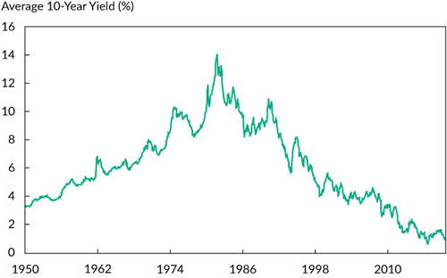
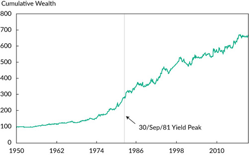
In the study reported in this article, we combined two unique features that allowed us to thoroughly study bond return predictability while overcoming these challenges. First, we used an extensive historical sample that spans all major government bond markets of developed countries over a 70-year period (January 1950–May 2019), thereby, generally, more than doubling the length of the sample commonly used in studies while also extending the sample size considerably in the cross section. In total, we have 7,497 monthly return observations in our sample, providing us with sizable testing power to examine bond return predictability. Moreover, in our sample period, global bond yields displayed two secular rate cycles, as illustrated by the development of the global average 10-year yield for the developed markets shown in Figure 1. Post-1980, global government bond yields displayed, roughly, a secular decline across the world. However, between 1950 and roughly 1980, the period that can be considered a new sample because it has not been studied before, yields displayed the opposite behavior (i.e., a secular rise). Therefore, our study also provides a natural robustness test of the influence of secular declining yields on bond return predictability.

Figure 1. Global Government Bond Yield Levels, January 1950–May 2019

Note: Shown are averages for the 10-year bond yields for Australia, Canada, Germany, Japan, the United Kingdom, and the United States.

Second, we describe a testing framework that centers around financial trading strategies instead of predictive regressions. By using a testing framework that builds upon trading strategies, we have a real-time assessment of the economic value of bond return predictability. At the same time, statistical significance tests of bond return predictability are easily embedded via the standard evaluation of the trading strategies’ performance. In addition, estimation problems of the predictive regressions’ critiques (e.g., overlapping data, persistent regressors) are overcome. Moreover, this trading-based framework allows us to examine explanations linked to transaction costs and other investment frictions—practical aspects that are highly relevant for practitioners.

To limit the risk of p-hacking in our study, we carried out our analysis in a unified testing framework that, to a large extent, minimizes the degrees of freedom. We focused on variables documented in previous studies for which coverage was available over our full sample period and for the markets we studied. To this end, we relied on studies by Ilmanen (1995, 1997), Yamada (1999), and Ilmanen and Sayood (2002). The variables we used are steepness of the yield curve (i.e., yield spread), past bond returns (i.e., bond trend), past equity returns, and past commodity returns; we also used their combination to study their joint forecasting power.³ We kept these variables and their definitions unchanged over our out-of-sample period to have a reliable and robust assessment of bond return predictability even in the wake of p-hacking.

We found consistent and ubiquitous evidence for bond market predictability, indicated by economically strong and generally statistically significant Sharpe ratios for each of the four variables and their (equal-weighted) model combination. The blue bars in Figure 2 summarize these results over the post-1980 period studied before, which, as shown in Figure 1, was mainly characterized by declining yields. The Sharpe ratio is a sizable 0.73 on the “Global” results for this in-sample period and is above 0.35 for every single country.

Figure 2. Sharpe Ratios for the Bond Market Predictability Strategy, 1981–2019 and 1950–1980

Note: The Sharpe ratios are for the four predictor variables per country and combined (the “Global” bars) split into in-sample (October 1981–May 2019) and out-of-sample (December 1949–September 1981) periods.

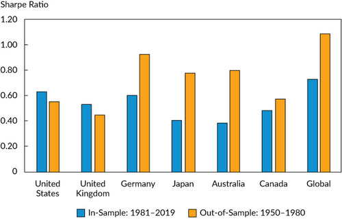
Interestingly, the results are similar for the 1950–80 “out-of-sample” period (the orange bars in Figure 2), characterized mainly by rising yields. Recall that we would expect to see no evidence of bond return predictability in the out-of-sample period if bond return predictability in the in-sample period were the result of a statistical Type I error (i.e., a false positive) or (an extreme level of) p-hacking. In contrast, a trading strategy based on bond return predictability would have achieved a remarkable 1.09 Sharpe ratio in the out-of-sample period. This result implies also that we found no significant evidence of an out-of-sample decay, as would be expected if the in-sample results were unduly influenced by p-hacking or other statistical effects. This finding stands in sharp contrast to out-of-sample findings on return anomalies in equity markets (see, e.g., Linnainmaa and Roberts 2018). For the full sample period (1950–2019), we found a substantial Sharpe ratio of 0.87.

To further explore robustness of the evidence supporting bond return predictability, we conducted several additional tests. First, we found the predictability to be robust in the subperiods in both our in-sample and out-of-sample periods, including, for example, the change from secular rising to secular declining yields; the predictability held for every decade since 1950. Second, the predictability is robust to several variations in testing choices, again providing evidence against a p-hacking explanation. Third, the predictability also held in a further out-of-sample test of the returns of nine additional developed government bond markets between January 1950 and May 2019. These results reveal that bond return predictability is a sizable and robust phenomenon in financial markets and is unlikely to be the result of data mining.

We next provide further insights into the economic channel of bond return predictability. One possible channel is that bond return predictability reflects a rational compensation for risk. Economic theory suggests that expected returns on bonds can vary as a result of perceived market risk or macroeconomic risk (Chen, Roll, and Ross 1986; Fama and French 1989; Ferson and Harvey 1991). Note that our long-term dataset is especially useful for examining this channel because it offers substantial variation in both market and macroeconomic risks—in contrast to more recent, shorter samples. In several tests, we found little supporting evidence for a risk-based explanation. Instead, bond return predictability seems to reflect a market inefficiency in the government bond market that can be exploited by market timing (a higher bond beta in rising markets than in falling markets), with higher performance coming in times of large market moves.

Finally, we examined the influence of investment frictions by exploring several practical applications of the documented bond return predictability. We found in asset allocation tests that investors benefit as the Sharpe ratio of the ex post mean–variance portfolio rises from 0.34 for a traditional equity/bond portfolio to 0.66 with inclusion of a simple bond market-timing portfolio. Furthermore, we document that bond predictability still holds after accounting for realistic levels of transaction costs. For example, we found a full-sample net Sharpe ratio of 0.71 and net Sharpe ratios of 0.91 and 0.58 for, respectively, the January 1950–September 1981 and October 1981–May 2019 subperiods. Moreover, we show strong evidence of bond market predictability in a subsample of highly liquid 10-year bond futures, for which taking short positions is easy. Finally, we show that the bond market–timing strategy adds substantial value for the bond market investor, also in a long-only context that avoids shorting or leverage. These results suggest that bond return predictability is not explained by investment frictions and, at the same time, that the timing of international bond market returns offers attractive and exploitable opportunities to investors.

Sample and Bond Market Predictors

In this section, we describe the variables we used, their construction, the testing methodology, and the dataset we used. We considered the 10-year government bonds of six major markets: the United States, the United Kingdom, Germany, Japan, Canada, and Australia. These markets are the major developed-market bond markets around the world with sufficient data coverage for the variables we studied. Moreover, 10-year bonds were available for our full history and are typically the most frequently considered and the most liquid part of the bond market, which is illustrated by the availability of highly liquid 10-year bond futures for these six markets. Note that we studied bond market predictability, which primarily originates from level shifts in bond yields (Litterman and Scheinkman 1991; Driessen et al. 2003), and therefore, our results should be representative of predictability for other parts of the bond yield curve. For predicting returns in the cross section of bond markets, see, amongst others, Asness, Moskowitz, and Pedersen (2013) and Koijen, Moskowitz, Pedersen, and Vrugt (2018), for which Baltussen, Swinkels, and van Vliet (forthcoming) provided deep historical evidence. For predicting returns across maturity buckets on the yield curve, see, amongst others, Martens, Beekhuizen, Duyvesteyn, and Zomerdijk (2019).

Motivated by Ilmanen (1995) and subsequent studies, we focused on predictor variables documented in previous studies for which coverage is available for our full sample period and for the markets we studied. The predictor variables we tested are yield spread, bond trend, equity returns, and commodity returns, which we defined as described in the following sections.

Yield Spread.

Yield spread is defined as the 10-year yield minus the cash rate. It is also known as the term spread, curve steepness, and slope factor. Dyl and Joehnk (1981), Fama (1984), Campbell and Shiller (1991), Ilmanen (1995, 1997), Yamada (1999), Ilmanen and Sayood (2002), and Duyvesteyn and Martens (2014)—all found strong predictive power for the yield spread, with a steep curve leading to higher future bond market returns. For international bond markets, a long history is available for both 10-year yields and cash rates.⁴ A related measure is the real yield—which compares the 10-year yield with past inflation or expected inflation based on forecasts. Because this measure correlates highly with the yield spread and requires either inflation survey data or vintage realized inflation data—neither of which is available from 1950 onward for six international bond markets—we chose to focus instead on the yield spread.

Bond Trend.

Bond trend is defined following Moskowitz et al. (2012), as the sign of the past 12-month bond return. The paper of Cutler, Poterba, and Summers (1990) was one of the first studies to test bond trend. It showed that past positive bond returns predict positive future bond returns. This paper was followed by Ilmanen (1997). Yamada (1999) applied bond trend to Japan, Ilmanen and Sayood (2002) applied it to Germany, and Luu and Yu (2012) to multiple developed markets as did Moskowitz et al. (2012), Duyvesteyn and Martens (2014), Hambusch, Hong, and Webster (2015), and Baltussen et al. (forthcoming).

Equity Return.

Equity return is defined as the past 12-month equity return in excess of cash. To the best of our knowledge, Ilmanen (1995) first proposed using past equity returns for predicting international bond returns. He found that negative past equity returns lead to positive future bond returns. Other studies are Ilmanen (1997) for the US market, Yamada (1999) for Japan’s market, and Ilmanen and Sayood (2002) for Germany’s market. Duyvesteyn and Martens (2014) used more than a decade of new data and more bond markets to provide out-of-sample evidence in the developed and emerging markets.

Commodity Return.

Commodity return is defined as the past 12-month commodity index return. Ilmanen and Sayood (2002) used the trend in commodity prices to predict German bond returns. Their idea was that

falling commodity prices signal disinflationary pressures, and should boost bond returns both contemporaneously and in the near future (given the observation that mild underreaction effects occur in many asset markets). (p. 41)

Ludvigson and Ng (2009) used principal components analysis on more than 100 macroeconomic series and found that the third and fourth factors load most heavily on measures of inflation and price pressure. These measures are, in turn, highly correlated with both commodity prices and consumer prices. We measured commodity returns as the Thomson Reuters/Core Commodity CRB Total Return Index; we used it as a proxy for inflationary pressures and tested it as a predictor of bond returns.

Data and Methodology

In the following subsections, we describe how we constructed our dataset, provide summary statistics for the six bond markets, explain the testing framework we developed, and describe the tests we conducted.

Dataset Construction.

We compiled our data from several sources to have a reliable and historically extensive dataset. Our prediction sample covers about 70 years of data, starting with the first prediction on 31 December 1949 and running until May 2019.⁵ The start date was chosen to include decades of rising yields while avoiding extreme events that could obscure bond market predictability inferences (e.g., World War II, the June 1948 German debt restructuring, and the hyperinflation years in Japan).

We obtained the most recent historical data on financial market prices from Bloomberg and Datastream, and we spliced them before inception with data from Global Financial Data. Global Financial Data constructs bond data from a combination of sources, which we describe in detail with series start and end dates in Appendix A. We used bond futures returns from their inception (1982 for the United States to 1990 for Germany), which we spliced before inception with returns on a representative bond (index) computed in excess of local financing rates. Note that these local excess returns are approximately equal to currency-hedged excess returns because the cost of currency hedging is, by arbitrage, directly related to the risk-free rate differential across countries. It does ignore the currency risk of unexpected profits or losses, however, which we embedded by denoting the excess returns in US dollars, but this effect is inherently a second-order effect (Ilmanen 2011). Futures returns are already equivalent to excess returns, so we did not deduct the risk-free rate. We rolled futures the day before first notice and ensured that returns correctly reflected the roll to prevent spurious effects.

Our sample is at the monthly frequency (using variables at the end of every month) and covers the major developed bond markets: Australia, Canada, Germany, Japan, the United Kingdom, and the United States. We used various data-quality checks to ensure a dataset of good quality, as further described in Appendix A. Because Japanese bond data between January 1950 and October 1961 are contaminated by the interpolation of yields, we started our sample of Japanese bond market returns in October 1961.

Figure 1 shows the average 10-year yield of the six countries. Most previous studies started after September 1981, the peak in Figure 1, meaning they looked only at a period of predominantly declining yields. In our study, we doubled the typical sample period, building a unique out-of-sample period of about 30 years for all major government bond markets. Interestingly, this period witnessed a secular increase in yield levels, thereby providing a natural robustness test of the influence of secular declining yields. Furthermore, bond markets and their economic and political landscapes have evolved considerably in these countries since the 1950s, with changing central bank policies (e.g., introduction of explicit inflation targeting, zero-interest-rate policies, and quantitative easing), the Cold War ending, other major political shifts (such as German reunification and the formation of the eurozone with its own central bank), and derivatives on bonds becoming key trading vehicles, to name a few.

Table 1 shows the performance statistics of the six bond markets over the January 1950–May 2019 period, the October 1981–May 2019 subperiod (a period with mostly declining yields), and the January 1950–September 1981 period (a period with mostly rising yields). When focusing on the global equal-weighted average over markets (the last column, “Global”), we found an average bond market return of –0.3% over the first subperiod and 3.9% over the latest subperiod.

Table 1. Summary Statistics for International Bond Market Returns

Performance Measure	Australia	Canada	Germany	Japan	UK	US	Global
A. October 1981–May 2019
Mean return	3.6%	4.2%	3.8%	3.2%	3.6%	4.7%	3.9%
Volatility	7.6%	7.0%	5.2%	4.7%	7.6%	6.9%	5.0%
Sharpe ratio	0.48	0.60	0.73	0.69	0.48	0.69	0.78
B. January 1950–September 1981
Mean return	–0.2%	–1.6%	1.9%	3.6%	–1.8%	–2.1%	–0.3%
Volatility	3.3%	5.1%	4.6%	7.0%	14.3%	6.0%	3.8%
Sharpe ratio	–0.06	–0.31	0.40	0.51	–0.12	–0.36	–0.07
C. January 1950–May 2019
Mean return	1.9%	1.6%	2.9%	3.4%	1.2%	1.6%	2.0%
Volatility	6.0%	6.3%	4.9%	5.6%	11.2%	6.6%	4.5%
Sharpe ratio	0.31	0.25	0.59	0.60	0.10	0.24	0.44

Notes: Returns and volatility are annualized. Returns are monthly excess returns. “Global” represents the equally weighted average of the six countries. Our sample for Japan begins October 1961.

Sources: Data are from Global Financial Data, Bloomberg, and Datastream.

Methodology.

To examine bond return predictability, we developed a testing framework centered around financial trading strategies instead of predictive regressions. This testing framework focuses directly on the economic value for an investor by building trading strategies and evaluating their performance as tests of our hypotheses.

We built the bond predictability trading strategies in the following manner. First, we took the predictor variables described previously and transformed each into a real-time trading signal. To limit the risk of p-hacking, we did so in a largely unified manner across variables such that degrees of freedom were minimized to a large extent. We also kept the definitions of the variables and the procedure we provide here unchanged for our full sample, hence, including the out-of-sample period. This step allowed us to make a reliable and robust assessment of bond return predictability even in the wake of p-hacking.

We transformed the predictor variables into a trading signal in the following manner. For the bond trend variable, we followed Moskowitz et al. (2012) and took the sign of the past 12-month excess bond return for each country, c, as the trading signal:

(1) $I_{Trend,c,t}=\left\{\begin{array}{c} 1 if {{\displaystyle \sum }}_{\tau =1}^{12}ERetur{n}_{c,t-\tau }>0\\ -1 if {{\displaystyle \sum }}_{\tau =1}^{12}ERetur{n}_{c,t-\tau }<0\end{array}\right.$ (1)

For the yield curve, equity return, and commodity return, we used the past 10 years of data and transformed the variable into a standardized z-score. More formally, (2) $z_{Variable,t}=Sig{n}_{Variable}\times \frac{Variabl{e}_t-{{\displaystyle \sum }}_{\tau =t-119}^{\tau =t}Variabl{e}_{\tau }/120}{\sqrt{{{\displaystyle \sum }}_{\tau =t-119}^{\tau =t}{\left(Variabl{e}_t-{{\displaystyle \sum }}_{\tau =t-119}^{\tau =t}Variabl{e}_{\tau }/120\right)}^2/120}},$ (2) where $Sig{n}_{Variable}$ is +1 for yield spread and –1 for equities and commodities, which is in line with the studies discussed in the previous section.⁶ For example, for the 12-month equity return variable, we deducted from the 12 months’ past equity return its average over the past 120 months (i.e., 10 years) and then divided it by the standard deviation over the same period. When a variable had fewer than 10 years of data available, we used data available up to that point, with a minimum of three years. To avoid extremes, we capped the z-scores at 1:

(3) ${\overline{z}}_{Variable,t}=\text{min}\left[1,\text{ max}\left(-1,z_{Variable,t}\right)\right].$ (3)

Before we continue, we want to stress that our results are generally robust to common variations on these choices, including using a z-score for bond trend (instead of its sign shown as in Equation 1 (1) $I_{Trend,c,t}=\left\{\begin{array}{c} 1 if {{\displaystyle \sum }}_{\tau =1}^{12}ERetur{n}_{c,t-\tau }>0\\ -1 if {{\displaystyle \sum }}_{\tau =1}^{12}ERetur{n}_{c,t-\tau }<0\end{array}\right.$ (1) ), using the sign of the scores as the trading signal for yield spread, equities, and commodities (instead of the raw z-score as shown in Equation 2 (2) $z_{Variable,t}=Sig{n}_{Variable}\times \frac{Variabl{e}_t-{{\displaystyle \sum }}_{\tau =t-119}^{\tau =t}Variabl{e}_{\tau }/120}{\sqrt{{{\displaystyle \sum }}_{\tau =t-119}^{\tau =t}{\left(Variabl{e}_t-{{\displaystyle \sum }}_{\tau =t-119}^{\tau =t}Variabl{e}_{\tau }/120\right)}^2/120}},$ (2) ), and also not capping the z-scores and using a five-year lookback period for computing z-scores, all of which are shown in numbers in Appendix B.

We also constructed a combined z-score for the four predictor variables to study joint forecasting power. To this end, we combined the four variables at the end of each month t for each country c:

(4) $Combine{d}_{c,t}={\overline{z}}_{Yield Spread,c,t}+{\overline{z}}_{Equities,c,t}+{\overline{z}}_{Commodities,c,t}+I_{Trend,c,t}.$ (4)

We assessed bond return predictability by evaluating the performance of the trading signals, updated monthly. In the next section, the size of the investment position is proportional to either the result for $Combine{d}_{c,t}$ or one of its components. The position is then multiplied by the next month’s excess bond returns to compute performance per market. We also computed a Global strategy performance by taking an equal-weighted average of strategy performances for all the countries; for example,⁷

(5) $ERetur{n}_{GLOBAL,t+1}=\frac{1}{C}{{\displaystyle \sum }}_{c=1}^{C}Combine{d}_{c,t}\cdot ERetur{n}_{c,t+1}.$ (5)

Equation 5 (5) $ERetur{n}_{GLOBAL,t+1}=\frac{1}{C}{{\displaystyle \sum }}_{c=1}^{C}Combine{d}_{c,t}\cdot ERetur{n}_{c,t+1}.$ (5) can also be applied to one of the four predictor variables to get a global return for an individual variable.

At this stage, we are ignoring transaction costs to focus on examining bond return predictability, not necessarily profitability. In the subsection “Investment Frictions and the Investor Perspective,” we examine the role of transaction costs and other investment frictions. To this end, we also considered a simplified trading strategy that requires little trading. In this strategy, we translated the model score, $Combine{d}_{c,t}$, into simple fixed-size long–short or neutral positions:

(6) $Positio{n}_{c,t}=\left\{\begin{array}{c}1 if Combine{d}_{c,t}>0\\ 0 if Combine{d}_{c,t}=0\\ -1 if Combine{d}_{c,t}<0\end{array}\right.$ (6)

For our hypotheses testing, we evaluated the time series of the strategy returns by using standard time-series tests. More specifically, we evaluated average returns, volatilities, Sharpe ratios, their significance (see Lo 2002), and the intercepts in the time-series regressions.

This approach brings a number of key benefits. First, it directly addresses economic value added because the returns can be interpreted as the returns on a trading strategy. As a result, testing hypotheses boil down to using standard time-series tests to test the returns on the trading strategies. Second, estimation uncertainty regarding parameters is avoided because the positioning is not dependent on rolling regressions. Third, in the spirit of Campbell and Thompson (2008), we imposed the direction of each predictor variable to be in line with previous studies and to be in the same direction at each point of our sample, thereby limiting degrees of freedom and imposing logical economic restrictions. Finally, we limited long or short biases by standardizing the predictor variables.

Key Empirical Results

We split our analysis into an in-sample period (October 1981–May 2019), which has been used partly by some previous studies and often for a single market, and a unique and independent out-of-sample period not studied before (January 1950–September 1981). We also considered the full sample period (January 1950–May 2019). Furthermore, we examined robustness of the findings over subperiods, sample choices, and tests of market-timing ability.

We start with the results of Combined_c,t (i.e., Equation 4 (4) $Combine{d}_{c,t}={\overline{z}}_{Yield Spread,c,t}+{\overline{z}}_{Equities,c,t}+{\overline{z}}_{Commodities,c,t}+I_{Trend,c,t}.$ (4) ) and its four components aggregated over the six countries to produce the Global strategy (i.e., Equation 5 (5) $ERetur{n}_{GLOBAL,t+1}=\frac{1}{C}{{\displaystyle \sum }}_{c=1}^{C}Combine{d}_{c,t}\cdot ERetur{n}_{c,t+1}.$ (5) ). As Table 2 shows, for the October 1981–May 2019 in-sample period, the Global strategy displays strong evidence of bond return predictability, with a Sharpe ratio of 0.73 and an annual excess return of 1.5%. Moreover, this predictability is present in each of the four predictor variables.

Table 2. Empirical Evidence on Bond Return Predictability: Global Sample

Performance Measure	Commodities	Equities	Yield Spread	Bond Trend	Combined
A. October 1981–May 2019
Mean return	1.3%	1.3%	1.1%	2.1%	1.5%
Volatility	3.9%	3.3%	2.9%	4.4%	2.0%
Sharpe ratio	0.34*	0.40**	0.38**	0.49**	0.73**
B. January 1950–September 1981
Mean return	1.6%	0.9%	2.0%	2.5%	1.8%
Volatility	2.5%	2.7%	3.1%	3.4%	1.7%
Sharpe ratio	0.63**	0.34*	0.64**	0.74**	1.09**
C. January 1950–May 2019
Mean return	1.5%	1.2%	1.5%	2.3%	1.6%
Volatility	3.3%	3.1%	3.0%	3.9%	1.9%
Sharpe ratio	0.44**	0.38**	0.50**	0.59**	0.87**

Notes: We applied four predictive variables and their combination (the Combined column; see Equation 4 (4) $Combine{d}_{c,t}={\overline{z}}_{Yield Spread,c,t}+{\overline{z}}_{Equities,c,t}+{\overline{z}}_{Commodities,c,t}+I_{Trend,c,t}.$ (4) ) to six bond markets, with monthly rebalancing. Shown are the average annualized return and volatility as well as Sharpe ratios when the performance of the long–short positions was aggregating to Global (see Equation 5 (5) $ERetur{n}_{GLOBAL,t+1}=\frac{1}{C}{{\displaystyle \sum }}_{c=1}^{C}Combine{d}_{c,t}\cdot ERetur{n}_{c,t+1}.$ (5) ); we took the average of the results for the six bond markets.

*Significant at the 5% significance level.

**Significant at the 1% significance level.

Interestingly, these results are very similar over the earlier sample period. As mentioned, the January 1950–September 1981 period is an out-of-sample test case because this period has not been covered by the previously mentioned studies, and it is a period in which the yield level displayed a secular rise, with the average return for the six bond markets of –0.30% (see Panel B in Table 1). Recall that we would expect to see no evidence of bond return predictability over the out-of-sample period if in-sample findings were the result of a statistical Type I error or (an extreme form of) p-hacking. For this period, however, we found a combined Sharpe ratio of 1.09 with an annual excess return of 1.8% for the Global strategy—levels exceeding the in-sample findings. This finding also implies that we found no significant evidence of an out-of-sample decay, as would be expected if the in-sample results were unduly influenced by p-hacking or other statistical effects. This result stands in sharp contrast to typical out-of-sample results (see, for example, Linnainmaa and Roberts [2018] for various equity anomalies) but is in line with the results of Baltussen et al. (forthcoming). Furthermore, as found for the in-sample period, all the predictive variables provide a significantly positive return for the predictability strategy, with all Sharpe ratios above 0.30 (see Table 2). We found the Sharpe ratio of the equally weighted Combined strategy to be much higher than that of each variable individually because correlations between the variable returns (not tabulated here) are close to zero (averaging to only 6%). Finally, over the full sample period, we found a Sharpe ratio of 0.87 and an annual excess return of 1.6% for the Global strategy.

Table 2 covers the portfolio of the six bond markets. Next, in Table 3, we show the results per country for the full sample period (in Appendix B, Table B1 provides the results for Combined_c,t per country for each subperiod). For all six-country × four-variable combinations, the Sharpe ratios are positive. The combined performance of the four variables has significant Sharpe ratios for all countries—from 0.46 for Australia to 0.74 for Germany. Moreover, the correlation between the strategy returns for the countries (not shown in Table 3) is, on average, 0.48. As a result, the Sharpe ratio for the combination of the six countries is highest (0.87 as shown in Table 2) because there are diversification benefits across the bond market predictability strategies in a global sample instead of in one particular country.

Table 3. Evidence on Bond Market Predictability per Country: Sharpe Ratios, January 1950–May 2019

Country	Commodities	Equities	Yield Spread	Bond Trend	Combined
Australia	0.09	0.27*	0.35**	0.31**	0.46**
Canada	0.28**	0.34**	0.29**	0.33**	0.52**
Germany	0.47**	0.05	0.32**	0.65**	0.74**
Japan	0.25*	0.17	0.21	0.48**	0.56**
UK	0.35**	0.21	0.17	0.20	0.47**
US	0.37**	0.29**	0.44**	0.36**	0.60**

Note: See the notes to Table 2.

*Significant at the 5% significance level.

**Significant at the 1% significance level.

Overall, we found strong evidence of bond market predictability for six major government bond markets in 70 years of data, including more than 30 years of new data. The size of the effect is substantial, as indicated by a full-sample Sharpe ratio of 0.87 for a strategy with limited average bond market exposure.

Next, we consider to what extent bond return predictability originates in market timing. For this purpose, we defined the global bond market returns as the average of the six individual bond market returns: (7) $ERetur{n}_{M,t}=\frac{1}{6}{{\displaystyle \sum }}_{c=1}^{6}ERetur{n}_{c,t}.$ (7) We regressed the returns of the Global strategy from Equation 5 (5) $ERetur{n}_{GLOBAL,t+1}=\frac{1}{C}{{\displaystyle \sum }}_{c=1}^{C}Combine{d}_{c,t}\cdot ERetur{n}_{c,t+1}.$ (5) on the global bond market returns (conditional on the returns being positive or negative):

(8) $ERetur{n}_{GLOBAL,t}=\alpha +{\beta }^{+}\max \left(0,ERetur{n}_{M,t}\right)+{\beta }^{-}\min \left(0,ERetur{n}_{M,t}\right)+{\epsilon }_t.$ (8)

We expected that if the predictability originates in market timing, the strategy will have a long bias in the positioning when the bond markets post positive returns and a short bias when the bond markets post negative returns. The results, shown in Table 4, confirm that this pattern is indeed the case. The strategy has, on average, a significantly positive bond beta of 0.22 in months in which bond returns are positive and a significantly negative bond beta of –0.13 in months in which bond returns are negative. The intercept becomes statistically insignificant and negative, illustrating that predictability is a reflection of correctly predicting the direction of the bond markets.⁸

Table 4. Bond Market Timing Test, January 1950–May 2019

$\alpha$	${\beta }^{+}$	${\beta }^{-}$
–0.53%	0.22**	–0.13**

Notes: Results of the regression in Equation 8 (8) $ERetur{n}_{GLOBAL,t}=\alpha +{\beta }^{+}\max \left(0,ERetur{n}_{M,t}\right)+{\beta }^{-}\min \left(0,ERetur{n}_{M,t}\right)+{\epsilon }_t.$ (8) , regressing the excess returns of the Global strategy as defined in Equation 5 (5) $ERetur{n}_{GLOBAL,t+1}=\frac{1}{C}{{\displaystyle \sum }}_{c=1}^{C}Combine{d}_{c,t}\cdot ERetur{n}_{c,t+1}.$ (5) on the global bond market, computed as the average of the six bond market excess returns as defined in Equation 7 (7) $ERetur{n}_{M,t}=\frac{1}{6}{{\displaystyle \sum }}_{c=1}^{6}ERetur{n}_{c,t}.$ (7) . Separate coefficients were used when the global bond market was positive (coefficient ${\beta }^{+}$) and negative (coefficient ${\beta }^{-}$).

**Significant at the 1% significance level.

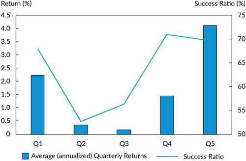
Finally, we checked in a nonparametrical way the dependency of our results for bond market predictability on whether the markets are up or down. We divided all the Global returns into five quintiles—from the worst returns (20% most negative calendar quarters) to the best (20% most positive). We subsequently computed for each quintile the contemporaneous average performance and its success ratio (i.e., the number of quarters it was positive) for the monthly rebalanced Global strategy as calculated in Equation 5 (5) $ERetur{n}_{GLOBAL,t+1}=\frac{1}{C}{{\displaystyle \sum }}_{c=1}^{C}Combine{d}_{c,t}\cdot ERetur{n}_{c,t+1}.$ (5) . Figure 3 shows that the strategy had very good predictive ability in both poor bond markets (quarterly return negative and below –1.4%) and in very strong bond markets (quarterly return positive and above 2.7%), confirming the results reported in Table 4. By contrast, predictability was substantially weaker, especially in the second quintile (Q2) and third quintile (Q3)—that is, if bond markets did not move much.

Figure 3. Bond Return Predictability Conditional on Bond Returns, January 1950–May 2019

Notes: Average (annualized) quarterly returns are shown on the left y-axis. The success ratio of the monthly rebalanced Global strategy in Equation 5 (5) $ERetur{n}_{GLOBAL,t+1}=\frac{1}{C}{{\displaystyle \sum }}_{c=1}^{C}Combine{d}_{c,t}\cdot ERetur{n}_{c,t+1}.$ (5) when sorted in quintiles based on the global bond market return in Equation 7 (7) $ERetur{n}_{M,t}=\frac{1}{6}{{\displaystyle \sum }}_{c=1}^{6}ERetur{n}_{c,t}.$ (7) is shown on the right y-axis.

Robustness Tests over Time, Settings, and an Additional Out-of-Sample Test.

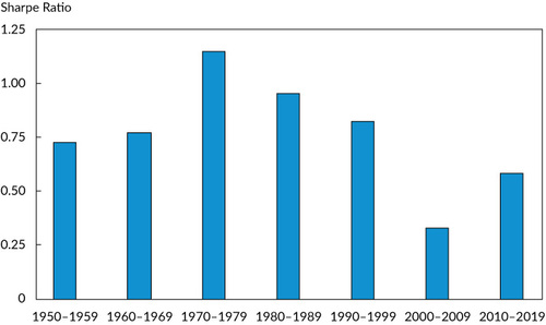
We conducted several robustness tests on the evidence of bond market return predictability. First, we divided our sample into calendar decades and used Equation 5 (5) $ERetur{n}_{GLOBAL,t+1}=\frac{1}{C}{{\displaystyle \sum }}_{c=1}^{C}Combine{d}_{c,t}\cdot ERetur{n}_{c,t+1}.$ (5) to compute the Sharpe ratio for the Global strategy for each decade (the last decade ended in May 2019). Figure 4 shows the results. Performance of the strategy was substantial each decade, with Sharpe ratios varying between 0.33 (for 2000–2009) to 1.15 (1970–1979). Moreover, performance was substantial for the last decade (a significant part of which also included new, untested data), as shown by a Sharpe ratio of 0.58.

Figure 4. Sharpe Ratios for Bond Market Timing per Decade, January 1950–May 2019

Note: Sharpe ratios of the Global strategy in Equation 5 (5) $ERetur{n}_{GLOBAL,t+1}=\frac{1}{C}{{\displaystyle \sum }}_{c=1}^{C}Combine{d}_{c,t}\cdot ERetur{n}_{c,t+1}.$ (5) .

Figure 5 provides further color on the robustness of performance over time by depicting the cumulative (gross of transaction costs) performance of bond market predictability for the Global strategy as calculated in Equation 5 (5) $ERetur{n}_{GLOBAL,t+1}=\frac{1}{C}{{\displaystyle \sum }}_{c=1}^{C}Combine{d}_{c,t}\cdot ERetur{n}_{c,t+1}.$ (5) for the full sample period. We observe stable and persistent evidence of bond market predictability across time.

Figure 5. Cumulative Performance of Bond Market Return Predictability Strategy, January 1950–May 2019

Note: The figure shows cumulative (gross) wealth of the global bond market predictability strategy in Equation 5 (5) $ERetur{n}_{GLOBAL,t+1}=\frac{1}{C}{{\displaystyle \sum }}_{c=1}^{C}Combine{d}_{c,t}\cdot ERetur{n}_{c,t+1}.$ (5) .

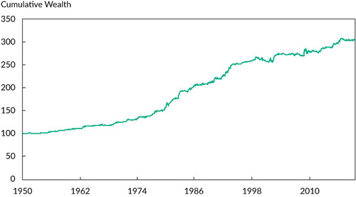
This finding does not critically depend on a secular decline in yields, as seen for the last 40 years. Noteworthy is that the predictability strategy also did well at the time of the big turning point in global bond yields around 1981, the structural change in stock–bond correlation observed over the 1977–87 period, and the 2007–09 Global Financial Crisis.

In a way, this result seems remarkable given how economic and political landscapes have evolved in these countries since the 1950s. For example, interest rates displayed a secular rise rather than decline, central bank policies evolved considerably, markets globalized, the Cold War ended, and major political shifts occurred, such as German reunification and the formation of the eurozone. The results suggest that these structural changes did not drive bond return predictability. That said, we stress that the results do not rule out the possibility that factors we are not considering affect results.

For our second robustness test, we considered robustness to testing choices. To start, we introduced an implementation lag of one month on the positions in Equation 4 (4) $Combine{d}_{c,t}={\overline{z}}_{Yield Spread,c,t}+{\overline{z}}_{Equities,c,t}+{\overline{z}}_{Commodities,c,t}+I_{Trend,c,t}.$ (4) . Hence, the model prediction at the end of month t was not applied to month t + 1 but to month t + 2, to allow for a delay in implementation and to remove any impact from a bid–ask bounce, stale pricing, misprints, or other measurement errors. The results are shown in Table B3 in Appendix B. The full-sample global model combination Sharpe ratio was 0.70, which is, again, highly significant in economic as well as statistical terms. Moreover, the full-sample and subsample results were found to be robust to variation in other testing choices, including not capping the z-scores, using z-scores for all variables (including bond trend), using the sign of the scores for each variable, and using a five-year lookback period to determine the scores.

Third, we considered robustness with respect to data quality. The deep historical data tend to be of lesser quality than the more recent data, as digital archives and the use of indexes with strong requirements on data processes did not exist. Instead, data were maintained typically by exchanges, statistical agencies, and newspapers. In Appendix A, we discuss potential data quality effects in more detail. Most notably, the timing of coupon payments was sometimes unknown, and as a solution, they were sometimes distributed to fixed points over the year, often year ends. Consequently, bond prices could artificially drop after coupon payments. To control for this effect, we also show robustness of the bond return predictability by reporting strategy returns by quarter, as shown in Table B4 in Appendix B. The findings align with those in Table 2, with strategy performance being generally significant over most quarters and not originating solely in the fourth quarter or any of the other quarters. These results provide further evidence against a p-hacking explanation of bond return predictability.

Fourth, we ran a further out-of-sample test on nine additional government bond markets, for which we obtained data from sources similar to those described in Appendix A. Our key focus was on the six main developed market countries, but we also collected data for the following European countries: Austria, Belgium, France, Italy, the Netherlands, Norway, Spain, Sweden, and Switzerland. These results, shown in Table 5, are remarkably similar to results for the six countries in our main sample. The full-sample Sharpe ratio equals 0.88 when the nine new countries are combined, compared with 0.87 for the original six countries. In the in-sample period (October 1981–May 2019), the Sharpe ratio is 0.76 for the nine new countries, compared with 0.73 for the six original countries. In the out-of-sample period (January 1950–September 1981), the Sharpe ratio is 1.28 for the nine additional countries, compared with 1.09 for the six original countries.⁹ In summary, bond market returns are also predictable in an additional sample of nine developed government bond markets.

Table 5. Bond Market Predictability for Nine Additional Countries, January 1950–May 2019

Country	Full Sample	In-Sample Subsample	Out-of-Sample Subsample
Austria	0.26*	0.48**	–0.01
Belgium	0.61**	0.53**	0.91**
France	0.66**	0.76**	0.53**
Italy	0.68**	0.48**	1.03**
Netherlands	0.77**	0.67**	0.87**
Norway	0.31**	0.27	0.36*
Spain	0.32**	0.48**	0.09
Sweden	0.26*	0.19	0.37*
Switzerland	0.75**	0.67**	1.07**
Global	0.88**	0.76**	1.28**

Notes: We applied the Combined_c,t model score as calculated in Equation 4 (4) $Combine{d}_{c,t}={\overline{z}}_{Yield Spread,c,t}+{\overline{z}}_{Equities,c,t}+{\overline{z}}_{Commodities,c,t}+I_{Trend,c,t}.$ (4) to nine additional bond markets.

*Significant at the 5% significance level.

**Significant at the 1% significance level.

All these results lead us to conclude that return predictability is a persistent and robust empirical phenomenon in bond markets, not driven by statistical Type I errors, data mining, or p-hacking effects.

Insights into the Economic Channels for Bond Return Predictability

The results discussed in the previous section reveal that bond return predictability is a sizable and robust phenomenon in financial markets and is unlikely to be the result of data mining or p-hacking. The question is, What is the economic channel of this predictability? We conjecture three classes of explanation for the bond return predictability: (1) a risk-based explanation, (2) market frictions, or (3) market inefficiency.

Risk-Based Explanation.

Risk-based explanations of return predictability argue that expected returns vary because of time variations in risk or risk premiums, aspects that can be expected to relate to macroeconomic or market conditions (Chen et al. 1986; Fama and French 1989; Ferson and Harvey 1991). Our long-term dataset was especially useful for examining this channel because it offered substantial variations in both market and macroeconomic risks as compared with only recent, shorter samples.

The simplest test was a check as to whether the bond market beta of the Global strategy from Equation 5 (5) $ERetur{n}_{GLOBAL,t+1}=\frac{1}{C}{{\displaystyle \sum }}_{c=1}^{C}Combine{d}_{c,t}\cdot ERetur{n}_{c,t+1}.$ (5) could explain the results. For that purpose, we ran the regression

(9) $ERetur{n}_{GLOBAL,t}=\alpha +\beta \cdot ERetur{n}_{M,t}+{\epsilon }_t.$ (9)

The results are reported in Table 6. Although we did find evidence for a slightly positive bond market beta of 0.07, it lowered the return per year only from 1.63% to 1.48% (the value of the intercept $\alpha$ in Equation 9 (9) $ERetur{n}_{GLOBAL,t}=\alpha +\beta \cdot ERetur{n}_{M,t}+{\epsilon }_t.$ (9) ). Hence, the bond risk premium explains only about 1/10 of the Global strategy returns, and the alpha of bond market predictability remains sizable and significant.

Table 6. Bond Beta, January 1950–May 2019

$\alpha \left(annualized\right)$	$\beta$
1.48%**	0.07**

Note: Results of the regression in Equation 9 (9) $ERetur{n}_{GLOBAL,t}=\alpha +\beta \cdot ERetur{n}_{M,t}+{\epsilon }_t.$ (9) , regressing the excess returns of the global strategy as defined in Equation 5 (5) $ERetur{n}_{GLOBAL,t+1}=\frac{1}{C}{{\displaystyle \sum }}_{c=1}^{C}Combine{d}_{c,t}\cdot ERetur{n}_{c,t+1}.$ (5) on the global bond market, computed as the average of the six bond market excess returns as defined in Equation 7 (7) $ERetur{n}_{M,t}=\frac{1}{6}{{\displaystyle \sum }}_{c=1}^{6}ERetur{n}_{c,t}.$ (7) .

**Significant at the 1% significance level.

Next, we examined predictability conditional upon the state of the economy. If predictability is driven by macroeconomic risks, we would expect it to be especially beneficial in good economic states but weak to absent in bad economic states (i.e., it gives exposure to bad states of the world). To test this conjecture, we constructed three sets of contemporaneous groups: inflation being above or below the median, the OECD Composite Leading Indicator being positive or negative,¹⁰ and bull versus bear equity markets. For each state, we computed the returns on the Global bond predictability strategy from Equation 5 (5) $ERetur{n}_{GLOBAL,t+1}=\frac{1}{C}{{\displaystyle \sum }}_{c=1}^{C}Combine{d}_{c,t}\cdot ERetur{n}_{c,t+1}.$ (5) . The results are shown in Table 7.

Table 7. Relationship of Bond Return Predictability to Economic States, January 1950–May 2019

	Inflation				Growth				Equity Returns
	Below Median	Above Median	Diff.		Low	High	Diff.		Below 0%	Above 0%	Diff.
Sharpe Ratio	0.66**	0.94**	0.28		1.02**	0.76**	0.26**		0.87**	0.67**	0.20

Notes: Returns are for the Global strategy as calculated in Equation 5 (5) $ERetur{n}_{GLOBAL,t+1}=\frac{1}{C}{{\displaystyle \sum }}_{c=1}^{C}Combine{d}_{c,t}\cdot ERetur{n}_{c,t+1}.$ (5) . Variables and markets were equally weighted. For inflation, we labeled each country-month observation as being below or above the median inflation and computed the average trading strategy performance for the countries below the median and those above the median. For growth, we followed the same procedure; we used the OECD Composite Leading Indicator, which identifies turning points regarding whether the global economy is slowing down (“Low”) or is expected to grow further (“High”). It starts in 1960, so we pre-filled it with NBER data on US recessions and expansions for 1950–1959. For equity returns, we used the average of the six countries and computed the average performance in equity quarters with returns below 0% and above 0%.

**Significant at the 1% significance level.

We found bond return predictability to be significantly stronger in a state of low economic growth than in the high-growth state, as shown by the significant difference in Sharpe ratio of 0.26 (1.02 compared with 0.76). Other measures do not display significant differences in Sharpe ratios between bad and good states. Overall, bond return predictability is consistently present and sizable in all economic states examined, as evident from the significantly positive Sharpe ratios—all exceeding 0.65. Thus, we conclude that our tests reveal no uniform evidence of a link between macroeconomic risks and bond return predictability.

In summary, the analyses show that macroeconomic risks cannot explain bond predictability and bond beta can, at best, explain a small fraction of the predictability. Consequently, our results are hard to reconcile with risk-based explanations, although we must be cautious in such an interpretation because risk exposures and, especially, risk premiums are not directly observable. For example, there may be hidden risk factors we do not know about. Instead, we interpret our findings as providing no positive evidence of a relationship between bond return predictability and risk.

Investment Frictions and the Investor Perspective.

We have shown consistent evidence for return predictability in a set of the major liquid government bond markets, and we have shown that this predictability is hard to align with risk-based explanations. A next question is, To what extent can the documented predictability be attributed to investment frictions? Most asset pricing models assume frictionless markets, although in reality investors face transaction costs, leverage constraints, practical or legal boundaries on shorting, and liquidity demands. The assumption of frictionless trading has been challenged in the literature, especially for stock-level factor premiums, which require high amounts of trading in illiquid stocks. For example, Korajczyk and Sadka (2004) examined the impact of frictions on the stock-level momentum factor, and Avramov, Chordia, and Goyal (2006) analyzed the stock-level short-term reversal factor. Novy-Marx and Velikov (2016) showed that simple trade rules are effective cost mitigation techniques and that most anomalies remain significant after transaction costs. To consider explanations related to investment frictions, we examined several practical applications of the documented bond return predictability: relevance for investor portfolios, the impact of transaction costs and liquidity, and the relevance of shorting bonds or applying leverage.

First, we asked whether bond return predictability is of practical relevance to global investors. To this end, we considered an optimal asset allocation problem in which we maximized the full-sample Sharpe ratio over global equities, global bonds, and a bond market–timing strategy, in which we required the portfolio weights to be nonnegative and to sum to unity (i.e., assuming an investor builds exposure via a fully funded position). The mean–variance optimal Sharpe ratio portfolio was invested 32% in the global equity market and 68% in the bond market, which yielded an annual Sharpe ratio of 0.34. When we added the bond market–timing strategy (imposing that portfolio weights sum to unity), its portfolio allocation became substantial, with a 50% weight, which increased the portfolio Sharpe ratio to 0.66. In other words, international bond market timing adds value for global investor portfolios, which is in line with the results presented in the sections “Key Empirical Results” and “Insights into the Economic Channels for Bond Return Predictability.”

Second, we considered transaction costs. We assumed one-way trading costs of 0.06% for our entire sample. In that assumption, we partially followed Hurst, Ooi, and Pedersen (2017), who assumed such costs for the period until 1992. They mentioned more recent estimates, however, to be 0.01%. Nevertheless, because these estimates are surrounded with substantial uncertainty, we chose to act on the more conservative side and assume 0.06% throughout our full sample. Table 8 shows the results. In the first two columns “Score (gross)” and “Score (net),” the results are for the Global strategy as defined in Equation 5 (5) $ERetur{n}_{GLOBAL,t+1}=\frac{1}{C}{{\displaystyle \sum }}_{c=1}^{C}Combine{d}_{c,t}\cdot ERetur{n}_{c,t+1}.$ (5) ; for the net results, we applied the one-way trading costs of 0.06%. The gross results are hardly affected; the full-sample Sharpe ratio drops from 0.87 in gross terms to 0.83 in net terms. We also took a complementary approach by computing the breakeven transaction costs, or the level of (one-sided) transaction costs at which the predictability would yield zero profitability. This number provides an upper bound on the level of transaction costs that the strategy allows to remain profitable in net terms. This number is 1.08%, 18 times the 0.06% we used, and arguably well above reasonable levels of actual transaction costs.

Table 8. Trading Strategy Net of Costs: Sharpe Ratios

Period	Score (gross)	Score (net)	Long–Short (gross)	Long–Short (net)
Full sample: 1950–5/2019	0.87**	0.83**	0.75**	0.71**
In-sample: 10/1981–5/2019	0.73**	0.69**	0.62**	0.58**
Out-of-sample: 1950–9/1981	1.09**	1.04**	0.95**	0.91**
Futures: 1990–5/2019	0.63**	0.58**	0.58**	0.53**

Notes: The results are for Global, with the average of the results for the six bond markets. “Score” is based on Combined as calculated in Equation 4 (4) $Combine{d}_{c,t}={\overline{z}}_{Yield Spread,c,t}+{\overline{z}}_{Equities,c,t}+{\overline{z}}_{Commodities,c,t}+I_{Trend,c,t}.$ (4) . For “Long–Short,” the position was set to +1 if the score was positive and to –1 if the score was negative (see Equation 6 (6) $Positio{n}_{c,t}=\left\{\begin{array}{c}1 if Combine{d}_{c,t}>0\\ 0 if Combine{d}_{c,t}=0\\ -1 if Combine{d}_{c,t}<0\end{array}\right.$ (6) ). The “net” includes one-way trading costs of 0.06%.

**Significant at the 1% significance level.

Third, because the previous strategy traded many small increments, we also considered a simple strategy as defined in Equation 6 (6) $Positio{n}_{c,t}=\left\{\begin{array}{c}1 if Combine{d}_{c,t}>0\\ 0 if Combine{d}_{c,t}=0\\ -1 if Combine{d}_{c,t}<0\end{array}\right.$ (6) . In this strategy, we took long, short, or neutral positions regardless of the size of the combined score. These results are shown in the last two columns of Table 8. Again, the Sharpe ratios remain large and significant. The in-sample and out-of-sample rows confirm that these results held for both periods. Figure B1 in Appendix B shows that the net performance of the long–short strategy was also consistent over time. These results suggest that bond market predictability is present even after accounting for transaction costs.

Fourth, the aforementioned trading strategies involved shorting bonds. Nowadays, shorting can be easily done by using futures, but this was significantly harder to do before the existence of futures markets. Moreover, bond markets were probably less liquid before the introduction of bond futures. To analyze whether predictability is driven by liquidity or short-selling constraints, we examined the strategy only for the sample period in which futures were available. The results are shown in the bottom row (“Futures”) of Table 8. Again, predictability remains economically and statistically strong, suggesting that neither short-selling constraints nor liquidity critically drove the documented predictability. Furthermore, as shown in Table 3, predictability was strong for (arguably) the most liquid market—namely, the US market—which provides further evidence that (il)liquidity does not critically drive predictability.

Finally, to explore the robustness to short selling further and to analyze other investment frictions, we considered two types of investor that would use the long–short (net) strategy: First, we assumed a 100% bond market investor, which allowed us to vary the duration of the portfolio investment in the bond market index between roughly zero (following a negative signal) and 2× the duration of the bond market index (following a positive signal). Second, we assumed a bond market investor that started with a 50%/50% cash/bond portfolio, and we varied the duration of this portfolio between 100% cash (following a negative signal) and 100% bonds (following a positive signal). Neither investor required short selling to implement their strategies, which, as noted, might have been tough in the distant past. Moreover, the cash/bond investor also did not require borrowing, which could be an investment friction in case of leverage constraints.

Table 9 shows the results. The Sharpe ratios on these portfolios increase from 0.44 to 0.74, and returns increase by 2.82 percentage points (pps) and 1.41 pps, respectively, suggesting neither short-selling constraints nor leverage constraints critically drive bond return predictability.

Table 9. Adding Bond Market Timing to a Bond Market Portfolio, 1950–May 2019

Performance Measure	100% Bonds	Add 100% of the Strategy	50% Cash/ 50% Bonds	Add 50% of the Strategy
Mean return	6.66%	9.48%	5.67%	7.08%
Volatility	4.52%	6.51%	2.26%	3.25%
Sharpe ratio	0.44	0.74	0.44	0.74

Notes: The table shows the Sharpe ratios for the global bond market (“100% bonds”), equally weighting the six countries (i.e., the final column in Table 1 apart from using total returns here for “Mean return” instead of excess returns over cash); the Market plus the Long–Short strategy in Table 8 as overlay (“Add 100% of the Strategy”), meaning we can go to 100% cash or 200% bonds; a 50% Cash/50% Bonds portfolio; and this 50/50 portfolio plus 0.5 times the Long–Short strategy as overlay, meaning we can go to 100% cash or 100% bonds. We include one-way trading costs of 0.06%. Because Sharpe ratios are using excess returns over cash, they are the same for the 100% and 50% cases.

The results in Table 9 indicate that bond market predictability is unlikely to be a reflection of investment frictions. Neither transaction costs nor the use of liquid instruments nor the prevention of shorting or leverage invalidated the documented bond return predictability. At the same time, these results imply that the predictability of international bond market returns could offer substantial value to investors.

That said, we acknowledge that without follow-up research on the specific shorting constraints and other investment frictions faced by an investor, our results do not necessarily imply that the documented predictability could have been profitably exploited by an investor. This study does not examine in depth smarter and possibly better definitions of the variables, smart trade rules, or aspects linked to (limits to) arbitrage and tradability (such as transaction costs and short-selling constraints). For example, introducing smart trade rules could reduce implementation costs significantly (see Novy-Marx and Velikov 2016). Investors do not need to have universal and frictionless access to all instruments in all markets, however, to profit from the predictability of bond returns. For example, even a long-only investor with access to a limited number of markets can postpone the buying of bonds if the particular market is in a negative trend or has a negative yield spread. In other words, investors could profit from the predictability to varying degrees. We leave a more elaborate assessment of positive predictability after costs and other investment frictions, or the design of an efficient investment strategy, for potential future research.

Market Inefficiency.

The results show that bond return predictability is a persistent empirical phenomenon in markets, one that is not driven by statistical Type I errors, data mining, or p-hacking. Furthermore, risk-based explanations and explanations related to market frictions are hard to reconcile with the results. Instead, we believe an explanation related to market inefficiency is best able to explain our results. This belief is in line with Moskowitz et al. (2012), who provided evidence favoring a behavioral explanation for one of our predictor variables—namely, bond trend—which they related to initial investor underreaction, delayed overreaction, and hedging pressures.

Two other results presented previously fit a market inefficiency explanation while being harder to align with a risk-based explanation. First, we found sizable Sharpe ratios, equaling 0.87 over the 1950–2019 sample period. The mere size of the finding suggests that bond return predictability does not result from rational compensation for risk. Rather, it seems to reflect a market inefficiency. Second, the results of the market-timing analyses as reported in Table 4 and Figure 3 reveal that predictability originates in correctly predicting both positive and negative bond returns. Admittedly, we may have overlooked a market efficiency explanation that is consistent with these sizable Sharpe ratios. However, regardless of the exact explanation, a rational time-varying risk explanation would be to align with both negative and positive expected bond returns if the government bond market is varying between a “hedge against” and an “amplifier of” aggregate consumption risk (see, for example, Campbell and Thompson 2008 and Driesprong, Jacobsen, and Maat 2008 for a related reasoning for equity market return predictability), which is empirically questionable in practice. In contrast, expected bond returns can vary from negative to positive if the predictability reflects a market inefficiency. That said, we stress that this story is a general one that is inherently hard to test, and therefore, we have to leave more testing of a market inefficiency explanation as an important avenue for future research.

Caveats

Our results show that bond return predictability is a sizable and robust phenomenon in financial markets—one that is unlikely to be the result of p-hacking or a risk-based explanation. It survives transaction costs and other investment frictions. These results emerged in a trading strategy–based testing framework, which thus implies potential value for investors. Next, we discuss several caveats to these findings.

First, our results reveal predictability of government bond markets over the short run; that is, we considered a monthly frequency for the trading strategies. Our main results reveal predictability over the next month ahead, although Table B3 reveals the results are robust to skipping an additional month. Therefore, exploiting the documented predictability would require substantial dynamics in bond positions. An open question is whether the results hold at a higher frequency, which we were unable to test thoroughly because of data availability over our out-of-sample period.

Second, our trading strategies take dynamic long and short positions over time with little structural market exposure and can be easily implemented in an unfunded manner via the use of bond futures. As such, the strategies can be easily added to passive fixed-income portfolios (as shown in, for example, Table 9). Added value over a passive government bond portfolio varied between 1.4 pps and 2.8 pps, so an active strategy would beat a passive strategy by combining static bond exposure with dynamic market timing. The value attained by adding the documented bond predictability to a passive strategy is most clear in the 1950–81 out-of-sample period, when the bond market provided a negative excess return (–0.3% in Table 1, Panel B). In that period, yield levels displayed a secular rise, and the dynamic trading strategy returned 1.8% (see Table 2, Panel B). The added value of bond market predictability was also present in the 1981–2019 in-sample period, however, when the bond market return was 3.9% (Table 1, Panel A) as yield levels displayed a secular decline, and the dynamic trading strategy returned 1.5% (Table 2, Panel A).

Third, the out-of-sample period, from 1950 to 1981, was dominated by rising yields, whereas the in-sample period, 1981–2019, was dominated by declining yields, as illustrated in Figure 1. Hence, both periods showed strong trends in yields, so one may wonder how this factor drives bond market predictability. For example, such strong trends are likely to benefit the bond trend variable. If yields in the future move in a range rather than the strong trending patterns seen in the past 70 years, the predictability of bond market returns could be less strong. On the one hand, as illustrated in Figure 3, predictability is strongest when bond markets move a lot—either up or down. On the other hand, we do observe that predictability has been consistent over time, including during the big turning point in global bond yields around 1981. Similarly, predictability turned out to be strongest in the 1950–81 period for Germany despite German interest rates trending upward much less strongly than those of the other countries, as evident from Tables 1 and B1.

Finally, several variables did not display significant bond return predictability for some individual markets (see Table 3). Such a pattern can also be expected in our alternative hypothesis, driven by sampling noise. Consequently, we chose not to focus on individual variable–country combinations in our results and refrained from studying differences in predictability across this dimension. Instead, we examined aggregate bond return predictability across the key global markets or across a set of predictor variables over a sample period spanning 70 years. Moreover, following previous studies, we imposed signs on the predictor variables ex ante. In practice, investors could argue for a dynamically changing sign—based on a rolling performance, for example. We leave the impact of this choice to future research.

Concluding Remarks

We found strong, robust, and persistent evidence of government bond return predictability in a deep sample spanning 70 years of international data across major developed bond markets. Economic profits were found to be sizable, with a global Sharpe ratio of 0.87 since 1950. Moreover, we found no evidence of out-of-sample decay of bond market predictability over a 30-year sample period between 1950 and 1980 or in nine additional government bond markets. The predictability is robust over time periods and market episodes, including prolonged periods of rising or falling rates. All these results cause us to conclude that bond return predictability is a persistent empirical phenomenon not driven by Type I errors, data mining, or p-hacking effects.

This question remains: What is driving the bond return predictability? Our tests reveal government bond return predictability neither seems to be driven by a risk-based explanation nor can be solely attributed to investment frictions, such as transaction costs and short-selling constraints. Instead, we believe bond return predictability is likely a manifestation of a market inefficiency. That said, regardless of the explanation, our results show that return predictability is a strong, robust, and persistent phenomenon in government bond markets across 70 years of data and 15 important bond markets.

These results imply that government bond returns display predictable dynamics. An interesting avenue for future research is the development of asset pricing theories that account for these predictable dynamics. From a practitioner perspective, the timing of international bond market returns offers substantial opportunities. Active management of government bonds, if successful, could add value by predicting the direction of yield changes.

Declaration of Interests

Disclosure: The authors report no conflicts of interest.

Notes

¹ P-hacking refers to the conscious or unconscious misuse of data analysis to find patterns in data. As a case in a point, Harvey, Liu, and Zhu (2016) found a clear publication bias in the top finance journals and found that of more than 300 documented stock-level anomalies, many became questionable after they were analyzed in a rigorous testing framework that allowed for multiple hypotheses testing bias. P-hacking is not limited to financial economics. It is mostly discussed in the social sciences and medicine. The Economist discussed the topic in 2013 under the title “How Science Goes Wrong.” Begley and Ellis (2012) showed that out of 53 studies on preclinical cancer, only 11% could be replicated. A 2015 open science collaboration showed that out of 97 significant psychological studies, only 36 could be replicated. In behavioral economics, Camerer, Dreber, Forsell, Ho, Huber, Johannesson, Kirchler, Almenberg, Altmejd, Chan, Heikensten, Holzmeister, Imai, Isaksson, Nave, Pfeiffer, Razen, and Wu (2016) found that out of 18 laboratory studies in economics, only 11 could be replicated with similar findings.

² In a related criticism, Boudoukh, Israel, and Richardson (2020) showed that predictive regressions focusing on long-run returns tend to be plagued by statistical issues because of the use of overlapping data. Furthermore, a large literature considers ordinary least-squares regressions of bond excess returns on the term structure of yields, which suffers from small-sample bias, size distortions, and serial correlation issues that exaggerate the degree of predictability (see, among others, Thornton and Valente 2012).

³ Note that requiring full coverage for 1950–2019 across several markets implies that we had to exclude variables based on survey data, combined macroeconomic series, and information from multiple bonds across the yield curve, as for example used by, respectively, Kim and Wright (2005), Ludvigson and Ng (2009), and Cochrane and Piazzesi (2005). These data sources typically did not have deep coverage in early history or in international markets. Moreover, macroeconomic data tend to be plagued by periodicity of issuance and revisions. For example, Ghysels, Horan, and Moench (2018) showed that bond return predictability based on macroeconomic data disappears when vintage data are used.

⁴ Note that this variable relates to Cochrane and Piazzesi (2005), who used a tent-shaped combination of forward rates across different maturities. Such a measure needs yields for other maturities, which are typically unavailable for a long history outside the United States.

⁵ Note that we used between 1 and 10 years of data before this period to construct the predictor variables.

⁶ Note that in this choice, we followed previous studies. In practice, investors could argue for a dynamically changing sign. Because our focus was on examining bond return predictability in-sample and out-of-sample with limited degrees of freedom, we leave this possibility to future research.

⁷ Note that the volatilities of the markets are not all equal, especially in the January 1950–September 1981 period (see Table 1). Consequently, this weighting scheme caused the higher-volatility markets to have more influence on the global strategy returns. We verified that our results were not driven by this choice; we witnessed, in general, higher global strategy returns in the January 1950–September 1981 period when, as an alternative, we weighed markets by their volatilities.

⁸ As an alternative, we also applied the Henriksson and Merton (1981) nonparametric test for market timing. This test considers the success ratio of predicting whether the excess bond return will be positive or negative; that is, it ignores how much is gained by correct predictions and lost by wrong predictions. The results of our nonparametric tests confirm the findings in Table 4. We found significant Henriksson and Merton test statistics for all individual markets and for three of the four individual variables (see Table B2 in Appendix B).

⁹ Note that several of these markets had become part of the eurozone as of 1999, which could have influenced the return dynamics in part of the in-sample period.

¹⁰ OECD recession indicators may be found at https://fred.stlouisfed.org/series/MSCRECM.

Appendix A.

Dataset Construction

Our sample covers 70 years of data from 31 December 1949 through 31 May 2019. We obtained the most recent historical data on financial market prices and macroeconomic series from Bloomberg and Datastream, which we spliced before inception with data from Global Financial Data.

Bonds

We sourced bond futures price and return data from Bloomberg, spliced these with bond index–level data from Datastream, and backfilled before inception with data from Global Financial Data. From the same sources, we obtained yields and inflation data. Table A1 shows the sample period and tickers used per data source.

Table A1. Bond Data Sources

	Australia	Canada	Germany	Japan	UK	US
A. Bond returns
GFD	1949–86 TRAUSGVM	1949–84 _TRCANGVM	1949–79 TRDEUGVM	1949–81 _TRJPNGVM	1949–79 TRGBRGVM	1949–79 _TRUSG10M
DS		1985–88 TCNGVG4(RI)	1980–89 TBDGVG4(RI)	1982–84 TJPGVG4(RI)	1980–81 TUKGVG4(RI)	1980–81 TUSGVG4(RI)
BB	1987–end XM1	1989–end CN1	1990–end RX1	1985–end JB1	1982–end G 1	1982–end TYI
B. 10-year bond yield
GFD	1949–86 IGAUS10D	1949–84 IGAUD10D	1949–79 IGDEU10D	1949–81 IGJPN10D	1949–79 IGGBR10D	1949–79 IGUSA10D
DS	1987–end TAUGV4(RA)	1985–end TCGVG4(RA)	1980–end TBDGVG4(RA)	1982–end TJPGVG4(RA)	1980–end TUKGVG4(RA)	1980–end TUSGVG4(RA)

Notes: GFD = Global Financial Data. DS = Datastream. BB = Bloomberg. For Bloomberg, we show the code of the index followed by the code of the Future 1st Contract.

Financing Rates

Our main measure for the financing rates was LIBOR (sourced from Bloomberg and Datastream), spliced with (in order of usage) Eurocurrency rates from Datastream, t-bill rates, and commercial paper yields from Global Financial Data. Table A2 shows the sample period and tickers used per data source.

Table A2. Financing Rates Data Sources

	Australia	Canada	Germany	Japan	UK	US
GFD	1949–85 ITAUS3D	1949–74 TRCANBIM	1949–74 ITDEU3D	1949–77 ITJPN3D	1949–74 ITGBR3D	1949–74 ITUSA3D
DS		1975–89 ECCAD1M	1975–85 ECWGM1M	1978–85 ECJAP1M	1975–85 ECUKP1M	1975–84 ECUSD1M
BB	1986–89 BBSW1M	1990–91 CDOR01	1999–end EE0001M	1986–end JY0001M	1986–89 BP0001M	1985–end US0001M
DS	1990–end BBAUD1M	1991–end BBCAD1M	1986–98 ECWGM1M		1989–end BBGBP1M

Notes: GFD = Global Financial Data. DS = Datastream. BB = Bloomberg. For Bloomberg, we show the code of the index followed by the code of the Future 1st Contract. Note that the 10-year yields from Table A1 and the financing rates from this table are combined to compute the term spread, 10Y–3M (10-year bonds minus 3-month bills).

Equities

We sourced price and return data of equity futures and indexes from Bloomberg, Datastream, and Global Financial Data. Our primary source was futures data from Bloomberg, with gaps filled in by Datastream data and spliced before futures inception with index-level data, as in Baltussen, Da, and Van Bekkum (2019). Next, we backfilled these data with equity index–level data downloaded from Global Financial Data. Table A3 shows the sample period and tickers used per data source.

Table A3. Equity Data Sources

	Australia	Canada	Germany	Japan	UK	US
GFD	1949–91 _AORDAD	1949–81 _TRGSPTSE	1949–58 _CDAXD	1949–50 _TOPXDVD	1949–81 GFUK100MRD	1949–50 _SPXTRD
BB	1992–end AS51, XP1	1982–end SPTSX60, PT1	1959–end DAX, GX1	1951–end TPX, TP1	1982–end UKX, Z 1	1951–end SPX, SP1

Notes: GFD = Global Financial Data. BB = Bloomberg. For Bloomberg, we show the code of the index followed by the code of the Future 1st Contract.

Commodities

We sourced return data on commodities from Global Financial Data. We used the Thomson Reuters/Core Commodity CRB Total Return Index (ticker: _CRBTRD), which spans our full sample period (1949–2019).

Data Quality

The deep historical data tend to be of lesser quality than more recent data because digital archives and the use of indexes with strong requirements for data processes did not exist for the early data. Instead, data were typically maintained by exchanges, statistical agencies, newspapers, and investor annuals. In the following, we highlight the potential data quality issues that could be at work and how we controlled for their effects.

• Misprints and other measurement errors. These errors could cause prices to be spuriously inflated, triggering potential reversals. In the robustness section, we show our robustness tests, which included a one-month implementation lag to control for this effect.

• Missing data points. This problem has sometimes been solved by interpolating, or padding, prices or returns known at a lower frequency to the monthly frequency. For example, bond prices are sometimes constructed on the basis of interpolated yields. We controlled for this issue by validating our data series and eliminating periods of interpolated data from our sample, which was the case for Japanese bond data between January 1950 and October 1961. Consequently, we begin our sample of Japanese bond market returns in October 1961.

• The timing of bond coupons. This information was not always known historically. As a solution, to construct return series, coupons have sometimes been distributed to fixed points over the year, often year ends. For bonds, this process causes a problem when bond prices are “dirty” (meaning the coupon is embedded in the price) because it causes artificial drops in bond prices after coupon payments. In the robustness section, we describe robustness tests that controlled for the resulting seasonality effects.

Appendix B.

Additional Results

Figure B1 shows the cumulative net performance of the strategy as calculated in Equation 6 (6) $Positio{n}_{c,t}=\left\{\begin{array}{c}1 if Combine{d}_{c,t}>0\\ 0 if Combine{d}_{c,t}=0\\ -1 if Combine{d}_{c,t}<0\end{array}\right.$ (6) .

Figure B1. Cumulative Performance of the Long–Short Strategy, Net of Transaction Costs, January 1950–May 2019

Note: The figure shows cumulative net wealth of the Long–Short Global bond market predictability strategy in Equation 6 (6) $Positio{n}_{c,t}=\left\{\begin{array}{c}1 if Combine{d}_{c,t}>0\\ 0 if Combine{d}_{c,t}=0\\ -1 if Combine{d}_{c,t}<0\end{array}\right.$ (6) .

Table B1 shows the bond market predictability results per country for the in-sample (post-October 1980) and the pre-sample (1950–September 1980) periods. Table B2 provides results of the Henriksson and Merton (1981) nonparametric market-timing test. Table B3 shows the robustness of primary results to testing choices. Table B4 provides the results per quarter as a robustness test of the impact of data quality.

Table B1. Bond Market Predictability Results per Country, January 1950–May 2019 and Subsamples

	Full Sample	In-Sample Subsample	Out-of-Sample Subsample
Australia	0.46**	0.38**	0.81**
Canada	0.52**	0.48**	0.57**
Germany	0.74**	0.60**	0.93**
Japan	0.56**	0.41**	0.78**
UK	0.47**	0.54**	0.45**
US	0.60**	0.63**	0.56**
Global	0.87**	0.73**	1.09**

Notes: Shown are Sharpe ratios for the Combined strategy as calculated in Equation 4 (4) $Combine{d}_{c,t}={\overline{z}}_{Yield Spread,c,t}+{\overline{z}}_{Equities,c,t}+{\overline{z}}_{Commodities,c,t}+I_{Trend,c,t}.$ (4) , with equally weighted variables. The full sample period is January 1950–May 2019, the in-sample period is October 1981–May 2019, and the out-of-sample period is January 1950–September 1981. The first column is also the final column in Table 3.

**Significant at the 1% significance level.

Table B2. Nonparametric Market-Timing Test

Australia	Canada	Germany	Japan	UK	US	Global
3.85**	1.85*	4.97**	2.83**	3.34**	2.75**	8.43**
Commodities	Equities	Yield Spread	Bond Trend
4.10**	1.45	3.31**	5.39**

Note: Reported are t-statistics for a Henriksson and Merton (1981) nonparametric test regarding the significance of market timing based on comparing how often the model correctly predicts the market return minus the risk-free rate: RM – rf ≤ 0 or RM – rf > 0.

*Significant at the 5% significance level.

**Significant at the 1% significance level.

Table B3. Robustness of Primary Results to Testing Choices: Global Portfolio, January 1950–May 2019

				Sharpe Ratios
	Trend Sign or z-Score	Other Variables	z-Scores Capped at 1	Full Sample	In-Sample Subsample	Out-of-Sample Subsample
Main result	sign	z-scores	yes	0.87**	0.73**	1.09**
Lag 1 month	sign	z-scores	yes	0.70**	0.58**	0.87**
No capping	sign	z-scores	no	0.79**	0.61**	1.03**
All scores	z-score	z-scores	yes	0.78**	0.58**	1.06**
All sign	sign	sign	—	0.75**	0.63**	0.96**
5-year z-score	sign	z-scores	yes	0.85**	0.70**	1.08**

Notes: The Global group combines all the countries; Sharpe ratios are as calculated in Equation 5 (5) $ERetur{n}_{GLOBAL,t+1}=\frac{1}{C}{{\displaystyle \sum }}_{c=1}^{C}Combine{d}_{c,t}\cdot ERetur{n}_{c,t+1}.$ (5) . The in-sample subsample spans October 1981–May 2019, and the out-of-sample subsample spans January 1950–September 1981. For the results shown in the row “Lag 1 month,” we delayed implementing the model outcome by one month. In the other rows, we varied the computation of the signals. For the main results described in the article, we used the sign for trend and used 10-year rolling z-scores for the other variables.

**Significant at the 1% significance level.

Table B4. Sharpe Ratios for the Global Portfolio per Quarter

	Full Sample	In-Sample Subsample	Out-of-Sample Subsample
All months	0.87**	0.73**	1.09**
1st quarter	0.91**	0.54**	1.36**
2nd quarter	0.40**	0.26	0.63**
3rd quarter	1.46**	1.51**	1.40**
4th quarter	0.73**	0.65**	0.89**

Notes: The Global group combines all the countries; Sharpe ratios are as calculated in Equation 5 (5) $ERetur{n}_{GLOBAL,t+1}=\frac{1}{C}{{\displaystyle \sum }}_{c=1}^{C}Combine{d}_{c,t}\cdot ERetur{n}_{c,t+1}.$ (5) . The full sample period is January 1950–May 2019, the in-sample period is October 1981–May 2019, and the out-of-sample period is January 1950–September 1981.

**Significant at the 1% significance level.

References

- Asness Clifford S. Tobias J. Moskowitz Lasse Heje Pedersen 2013 Value and Momentum Everywhere Journal of Finance 68 3 929 85
- Avramov Doron Tarun Chordia Amit Goyal 2006 The Impact of Trades on Daily Volatility Review of Financial Studies 19 4 1241 77
- Baltussen Guido Zhi Da Sjoerd Van Bekkum 2019 Indexing and Stock Market Serial Dependence around the World Journal of Financial Economics 132 1 26 48
- Baltussen Guido Laurens Swinkels Pim van Vliet Forthcoming Global Factor Premiums Journal of Financial Economics
- Bauer Michael D. James D. Hamilton 2018 Robust Bond Risk Premia Review of Financial Studies 31 2 399 448
- Begley C. Glenn Lee M. Ellis 2012 Drug Development: Raise Standards for Preclinical Cancer Research Nature 483 531 33
- Boudoukh Jacob Ronen Israel Matthew P. Richardson 2020 Biases in Long-Horizon Predictive Regressions Working paper, NYU Stern School of Business 28 May
- Camerer Colin F. Anna Dreber Eskil Forsell Teck-Hua Ho Jürgen Huber Mangus Johannesson Michael Kirchler Johan Almenberg Adam Altmejd Taizan Chan Emma Heikensten Felix Holzmeister Taisuke Imai Siri Isaksson Gideon Nave Thomas Pfeiffer Michael Razen Hang Wu 2016 Evaluating Replicability of Laboratory Experiments in Economics Science 351 6280 1433 36
- Campbell John Y. Robert J. Shiller 1991 Yield Spreads and Interest Rate Movements: A Bird’s Eye View Review of Financial Studies 58 3 495 514
- Campbell John Y. Samuel B. Thompson 2008 Predicting Stock Returns Out of Sample: Can Anything Beat the Historical Average? Review of Financial Studies 21 4 1509 31
- Chen Nai-Fu Richard Roll Stephen A. Ross 1986 Economic Forces and the Stock Market Journal of Business 59 3 383 403
- Cieslak Anna Pavol Povala 2015 Expected Returns in Treasury Bonds Review of Financial Studies 28 10 2859 901
- Cochrane John H. Monika Piazzesi 2005 Bond Risk Premia American Economic Review 95 1 138 60
- Cooper Ilan Richard Priestley 2009 Time-Varying Premiums and the Output Gap Review of Financial Studies 22 7 2801 33
- Cutler David James Poterba Lawrence Summers 1990 Speculative Dynamics and the Role of Feedback Traders American Economic Review 80 2 63 68
- Doeswijk Ronald Trevin Lam Laurens A. P. Swinkels 2020 Historical Returns of the Market Portfolio Review of Asset Pricing Studies 10 3 521 67
- Driesprong Gerben Ben Jacobsen Benjamin Maat 2008 Striking Oil: Another Puzzle? Journal of Financial Economics 89 2 307 27
- Driessen Joost Bertrand Melenberg Theo Nijman 2003 Common Factors in International Bond Returns Journal of International Money and Finance 22 5 629 56
- Duyvesteyn Johan Martin Martens 2014 Emerging Government Bond Market Timing Journal of Fixed Income 23 3 36 49
- Dyl Edward A. Michael D. Joehnk 1981 Riding the Yield Curve: Does It Work? Journal of Portfolio Management 7 3 13 17
- Fama Eugene F. 1984 The Information in the Term Structure Journal of Financial Economics 13 4 509 28
- Fama Eugene F. Kenneth R. French 1989 Business Conditions and Expected Returns on Stocks and Bonds Journal of Financial Economics 25 1 23 49
- Ferson Wayne E. Campbell R. Harvey 1991 The Variation of Economic Risk Premiums Journal of Political Economy 99 2 385 415
- Ghysels Eric Casidhe Horan Emanual Moench 2018 Forecasting through the Rearview Mirror: Data Revisions and Bond Return Predictability Review of Financial Studies 31 2 678 714
- Greenwood Robin Dimitri Vayanos 2014 Bond Supply and Excess Bond Returns Review of Financial Studies 27 3 663 713
- Hambusch Gerhard Kihoon J. Hong Ellenora Webster 2015 Enhancing Risk-Adjusted Return Using Time Series Momentum in Sovereign Bonds Journal of Fixed Income 25 1 96 111
- Harvey Campbell R. 2017 Presidential Address: The Scientific Outlook in Financial Economics Journal of Finance 72 4 1399 440
- Harvey Campbell R. Yan Liu Heqing Zhu 2016 . . . and the Cross-Section of Expected Returns Review of Financial Studies 29 1 5 68
- Henriksson Roy D. Robert C. Merton 1981 On Market Timing and Investment Performance II: Statistical Procedures for Evaluating Forecasting Skills Journal of Business 54 4 513 33
- Hurst Brian Yao Hua Ooi Lasse H. Pedersen 2017 A Century of Evidence on Trend-Following Investing Journal of Portfolio Management 44 1 15 29
- Ilmanen Antti 1995 Time-Varying Expected Returns in International Bond Markets Journal of Finance 50 2 481 506
- Ilmanen Antti 1997 Forecasting U.S. Bond Returns Journal of Fixed Income 7 1 22 37
- Ilmanen Antti 2011 Expected Return: An Investor’s Guide to Harvesting Market Rewards Hoboken, NJ Wiley Finance
- Ilmanen Antti Rafey Sayood 2002 Quantitative Forecasting Models and Active Diversification for International Bonds Journal of Fixed Income 12 3 40 51
- Joslin, Scott , Marcel Priebsch, and Kenneth J. Singleton 2014 Risk Premiums in Dynamic Term Structure Models with Unspanned Macro Risksh Journal of Finance 69 3 1197 233
- Kim Don H. Jonathan H. Wright 2005 An Arbitrage-Free Three-Factor Term Structure Model and the Recent Behavior of Long-Term Yields and Distant-Horizon Forward Rates Federal Reserve Board Finance and Economics Discussion Series (FEDS) Working Paper 2005-33 August
- Koijen Ralph S. J. Tobias J. Moskowitz Lasse Heje Pedersen Evert B. Vrugt 2018 Carry Journal of Financial Economics 127 2 197 225
- Korajczyk Robert A. Ronnie Sadka 2004 Are Momentum Profits Robust to Trading Costs? Journal of Finance 59 3 1039 82
- Linnainmaa J. T. M. R. Roberts 2018 The History of the Cross Section of Stock Returns Review of Financial Studies 31 7 2606 49
- Litterman Robert José Scheinkman 1991 Common Factors Affecting Bond Returns Journal of Fixed Income 1 1 54 61
- Lo Andrew W. 2002 The Statistics of Sharpe Ratios Financial Analysts Journal 58 4 36 52
- Ludvigson Sydney C. Serena Ng 2009 Macro Factors in Bond Risk Premia Review of Financial Studies 22 12 5027 67
- Luu Bac Van Peiyi Yu 2012 Momentum in Government Bond Markets Journal of Fixed Income 22 2 72 79
- Martens Martin Paul Beekhuizen Johan Duyvesteyn Casper Zomerdijk 2019 Carry Investing on the Yield Curve Financial Analysts Journal 75 4 51 63
- Moskowitz Tobias J. Yao Hua Ooi Lasse Heje Pedersen 2012 Time Series Momentum Journal of Financial Economics 104 2 228 50
- Novy-Marx Robert Mihail Velikov 2016 A Taxonomy of Anomalies and Their Trading Costs Review of Financial Studies 29 1 104 47
- Sarno Lucio Paul Schneider Christian Wagner 2016 The Economic Value of Predicting Bond Risk Premia Journal of Empirical Finance 37 247 67
- Thornton Daniel L. Giorgio Valente 2012 Out-of-Sample Predictions of Bond Excess Returns and Forward Rates: An Asset Allocation Perspective Review of Financial Studies 25 10 3141 68
- Yamada Satoshi 1999 Risk Premiums in the JGB Market and Application to Investment Strategies Journal of Fixed Income 9 2 20 41