Redefining the Optimal Retirement Income Strategy

Abstract

This paper introduces a cohesive series of models designed to improve retirement income projections. First, the retirement income goal (i.e., liability) is decomposed based on assumed spending elasticity (e.g., “needs” and “wants”). Second, spending is assumed to evolve throughout retirement using a dynamic withdrawal strategy leveraging the funded ratio concept. Third, optimal strategies are determined using an expected utility model based on prospect theory, which also yields a client-friendly outcomes metric. Overall, this framework can result in advice and guidance that is notably different than models using more basic (and common) assumptions, especially approaches relying on probability of success-related metrics.

Keywords:

• financial planning
• retirement
• wealth management

PL Credits: 0.75:

Retirement is seldom as simple as assumed in research and financial planning tools. Too often, the retirement spending goal is assumed to be some constant (static) amount, in today’s dollars (i.e., in real terms), where the efficacy of a given strategy is determined using metrics such as probability of success, which is the frequency with which the goal is completely accomplished in a given simulation. These flawed assumptions can result in estimates for required savings or retirement spending in research and financial planning tools that are significantly different than if a more realistic model is used.

In this paper, a cohesive series of models are introduced that are designed to improve retirement income projections. The models in this research are far more evolutionary, rather than revolutionary, given the decades of existing research in the retirement income space on these topics. This research is primarily focused on functional implementation, where the respective models introduced are designed to specifically address some of the more obvious shortfalls in existing models in a way that can be realistically (and practically) implemented.

First, we decompose the retirement spending goal (liability) into two separate goals: needs and wants, which reflects the fact that retirees typically have varied levels of elasticity (or required certainty) associated with different types of expenditures. For example, spending on travel is generally more flexible than spending on healthcare. Second, we introduce a model where spending levels (i.e., portfolio withdrawals) evolve throughout retirement based on how the retiree’s funded ratio (i.e., financial situation) changes over time. This approach can explicitly incorporate nonconstant cash flows, which is a key weakness of most existing approaches. Third, an expected utility model based on prospect theory is introduced to determine optimal strategies that better capture the expected satisfaction associated with accomplishing different levels of spending in retirement. The certainty-equivalent spending estimate from our utility model (the “goal completion score”) is a client-friendly outcomes metric that can be used to relay the efficacy of a given strategy to a household.

Overall, this analysis suggests that approaches that more accurately capture the retirement liability can result in advice and guidance that is notably different than models using more basic (and common) assumptions, especially approaches relying on probability of success-related metrics. Collectively, this research provides a framework that can help households make better decisions about retirement-related issues such as optimal spending levels, optimal portfolio risk levels, and optimal allocations to guaranteed income.

Redefining the Retirement Income Goal

Early research on retirement spending predominately focused on estimating “safe” initial withdrawal rates. Bengen’s (1994) research on the “4% Rule” is perhaps the most widely known example.¹ With initial withdrawal rates, the noted percentage is multiplied by the respective balance and that initial withdrawal amount (not the initial percentage) is assumed to be withdrawn from the portfolio for the duration of retirement (i.e., 30 years), typically adjusted annually for inflation. For example, with a 4% initial withdrawal rate, if the balance at retirement is $1 million, the withdrawal in the first year of retirement would be $40,000 and that initial amount ($40,000) would be increased by inflation until death.

Past research determining optimal portfolio withdrawal rates has generally used some type of stochastic (i.e., random) component, typically with respect to the return series, based on actual historical time-series data or some type of Monte Carlo simulation. Early research predominately relied on historical U.S. returns, although more recent research has considered international time-series data (e.g., Pfau 2010). There has also been an increased focus on using expected (or forecasted) returns given the relatively low interest rate environment today (e.g., Fink, Pfau, and Blanchett 2013).

Optimal outcomes in financial planning tools are typically determined based on achieving some acceptable probability of success (e.g., 90%), which is defined by the user. The probability of success is the percentage of runs (or trials) where the retiree accomplishes the respective retirement goal. Probability-of-success metrics completely ignore the magnitude of failure, which is a notable weakness of the metric.

Portfolio withdrawals, which are assumed to reflect retiree spending, are generally static and change only based on inflation and are not adjusted based on portfolio performance. This is obviously overly simplistic and consistent with life-cycle consumption smoothing only under a very limited set of implausible preference parameters (Milevsky and Huang 2011). In reality, retirees headed toward certain ruin (i.e., portfolio depletion) would likely adjust withdrawals to prolong the life of the portfolio.

A number of concepts that are commonly used when modeling retiree liabilities and determining optimal retirement strategies have been borrowed from best practices in the defined benefit (DB) space (e.g., the concept of liability driven investing, or LDI). Unlike in DB plans, though, which have “hard” liabilities that are legally mandated, retirees typically have some control over expenses (i.e., they could be perceived as “soft,” to some extent, as discussed by Idzorek and Blanchett [2019]). In other words, retirees typically have the ability to cut back on spending as situations warrant.

The “pain” associated with cutting back on spending depends to some extent on the respective expenditure. While some expenditures, such as healthcare, may be relatively painful for retirees to scale back on (and would therefore be considered relatively inelastic), other expenditures, such as travel, could be reduced more easily as situations warrant (and would be considered more elastic). Therefore, understanding the composition of retiree spending is important when assessing the efficacy of the common modeling assumption that all retiree expenditures are inelastic.

To better understand the composition of retiree expenditures, data from the 2020 Interview file of the Consumer Expenditure Survey (CES)² was reviewed. The analysis only includes respondents between the ages of 65 and 80 (inclusive) where the household is coded as being retired. Expenditures are categorized as being either elastic or inelastic. Figure 1 includes the average percentage of total household expenditures that are estimated to be inelastic for various total expenditure groups.

Figure 1. Inelastic Expenditures as a Percentage of Total Expenditures

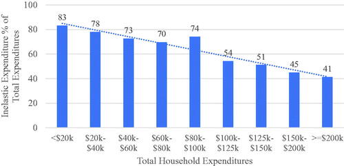
While approximately 65% of total retiree expenditures are estimated to be inelastic (i.e., “needs”), on average, households with higher total expenditures clearly have higher allocations to more elastic expenditures, on average (i.e., the more retirees spend, the more flexibility they appear to have with respect to what they are spending money on). There is also an increasing level variability in the breakdown of inelastic expenditures as total expenditures increase.

While these findings are not especially novel, since it is intuitive that some degree of retiree spending should be flexible, relatively few financial planning tools explicitly incorporate the notion of spending flexibility into the retirement forecast. In other words, financial planning tools overwhelmingly assume that retirees are unable and unwilling to adjust spending throughout retirement, despite relatively straightforward evidence to the contrary, especially among households with higher expenditures levels (who are more likely to use financial advisors).

While there are decades of research exploring various approaches to adjusting portfolio withdrawals over time, commonly referred to as dynamic spending (or withdrawal) rules, these approaches are generally difficult to implement and can significantly complicate financial planning tools. For example, when implementing some type of dynamic spending approach, not only do a series of rules need to be developed to determine how spending should (or will) evolve over time, but the outcomes metric also needs to be able to incorporate a range of potential scenarios, which “break” more common binary metrics, like the probability of success.

The unique contribution of this research to the literature is that it attempts to address these various retirement modeling issues simultaneously in a relatively straightforward series of cohesive models.

Dynamic Spending

The literature on dynamic spending rules has evolved over the last few decades and can generally be split into two groups. For the first group, the emphasis is on the rules themselves: Bengen (2001) suggests a floor/ceiling approach; Pye (2001) suggests withdrawing the lower of the previous amount (in real terms) or the amortized current portfolio value using the length of the remaining distribution period and expected portfolio rate of return; Guyton (2004) suggests guardrails; Stout and Mitchell (2006) develop a model based on both portfolio performance and remaining life expectancy; and Blanchett and Frank (2009) link adjustments to the ongoing likelihood of failure.

Recently, Waring and Siegel (2015, 2018) utilized an intertemporal budget constraint, accompanied by a regularly recalculated spending amount, to develop a fairly simple spending approach with little or no chance of ruin. The budget constraint, coupled with revisiting the annuitization decision annually, allows this method to incorporate volatile portfolios that are invested in risky assets.

The other line of early research on spending is quite different in its origin, coming out of stochastic dynamic-programming and utility-maximizing (life cycle) models, often in the context of the intertemporal asset pricing literature. One of the earliest life cycle models was developed by Merton (1969). Another example is Rubinstein’s model (1976), which explicitly derives a spending rule in the multi-period asset pricing context. While many of the dynamic spending models appear in the context of asset pricing, there are some that were developed explicitly for the spending problem, notably Milevsky and Huang (2011) and Habib, Huang, and Milevsky (2017).

Relatively few, if any, of the dynamic withdrawal rules that have been introduced in past research have actually been implemented in financial planning tools used today. This can largely be attributed to the fact that the approaches are either too computationally complex or they cannot handle the myriad of household situations that exist in real life (or both). The existence of nonconstant cash flows significantly increases the complexity of a simulation. For example, a scenario with spouses retiring at different ages, claiming Social Security benefits at different ages, and receiving future sources of guaranteed income (e.g., a longevity annuity starting at age 85) is something that most dynamic spending rules are simply not designed to consider.

In summary, while many dynamic spending rules have been developed for research purposes, they are not robust enough to capture the actual varied situations for retiree households that exist in the real world. Our dynamic spending rule is specifically designed to be robust enough to capture the varied situations (and cash flows) of retirees while being something that can be implemented in practice. The model is based on the concept of the “funded ratio,” which is conceptually similar to an approach introduced by Kaplan and Blanchett (2021).

The funded ratio is a metric commonly used to describe the health of pension plans, but it can more generally be used to estimate the overall financial situation for any goal (i.e., retiree consumption). The funded ratio is the total value of the assets, which includes both current balances and future expected income, divided by the liability, which would be all current and future expected spending. A funded ratio of 1.0 would imply that an individual has just enough assets to fully fund that goal. A funded ratio greater than 1.0 implies that the individual has a surplus, while a funded ratio of less than 1.0 implies that an individual has a shortfall.

For our analysis, we estimate funded ratios for two goals: “needs” (inelastic) spending and “wants” (elastic) spending. The model could easily be expanded to consider additional spending goals (e.g., “wishes” and/or “dreams”) if further differentiation is desired.

More technically, the formula used to estimate the needs funded ratio (${N\_FR}_t$) is included in Equation (1)(1) $${N\_FR}_t=\mathrm{ }\frac{A_t\hspace{0.17em}+\sum _{t=0}^T\frac{{cp}_t^s{P}_t}{{(1+r_p)}^t}}{\sum _{t=0}^T\frac{{cp}_t^s{n\_\hspace{0.17em}g}_t}{{(1+r_n)}^t}}$$(1) , where $T$ is the total number of simulation years; $A_t$ is total portfolio value at year $t;$ ${cp}_t^s$ is the cumulative probability of surviving to year $t;$ $P_t$ includes all future inflows, which are primarily assumed to be pension benefits such as Social Security retirement benefits; $n\_g_t$ is the assumed needs income goal for that specific year ($t$); and $r$ is the assumed discount rate (which can vary by cash flow). (1) $${N\_FR}_t=\mathrm{ }\frac{A_t\hspace{0.17em}+\sum _{t=0}^T\frac{{cp}_t^s{P}_t}{{(1+r_p)}^t}}{\sum _{t=0}^T\frac{{cp}_t^s{n\_\hspace{0.17em}g}_t}{{(1+r_n)}^t}}$$(1)

The wants funded ratio (${W\_FR}_t$), which is included in Equation (2)(2) $${W\_FR}_t=\mathrm{ }\max \left(\frac{A_t+\mathrm{ }\sum _{t=0}^T\frac{{cp}_t^s{P}_t}{{(1+r_p)}^t}-\mathrm{ }\sum _{t=0}^T\frac{{cp}_t^s{n\_g}_t}{{(1+r_n)}^t}}{\sum _{t=0}^T\frac{{cp}_t^s{w\_\hspace{0.17em}g}_t}{{(1+r_w)}^t}},0\right)$$(2) , is conceptually identical to the needs funded ratio calculation (in Equation (1)(1) $${N\_FR}_t=\mathrm{ }\frac{A_t\hspace{0.17em}+\sum _{t=0}^T\frac{{cp}_t^s{P}_t}{{(1+r_p)}^t}}{\sum _{t=0}^T\frac{{cp}_t^s{n\_\hspace{0.17em}g}_t}{{(1+r_n)}^t}}$$(1) ), but the assets available to fund the wants spending goal ($w\_g$) are reduced by the needs income goal liability. (2) $${W\_FR}_t=\mathrm{ }\max \left(\frac{A_t+\mathrm{ }\sum _{t=0}^T\frac{{cp}_t^s{P}_t}{{(1+r_p)}^t}-\mathrm{ }\sum _{t=0}^T\frac{{cp}_t^s{n\_g}_t}{{(1+r_n)}^t}}{\sum _{t=0}^T\frac{{cp}_t^s{w\_\hspace{0.17em}g}_t}{{(1+r_w)}^t}},0\right)$$(2)

The initial spending level for each of the two goals (needs and wants) would be based on their respective portion of the total retirement goal. For example, if the initial retirement income goal was $100,000, of which 70% is assumed to be needs, the initial “needs” withdrawal amount would be $70,000 and the initial “wants” withdrawal amount would be $30,000. Those spending amounts could evolve in future years based on the adjustments applied to the respective target values or other key assumptions (e.g., inflation).

This research uses relatively simple spending adjustment schedules to adjust needs and wants spending throughout the simulation. The needs goal is assumed to be completely inelastic and increases only with inflation annually (i.e., does not vary depending on portfolio performance). This replicates how the entire retirement spending goal is commonly modeled today (i.e., effectively static in real terms) and is consistent with more general pension liabilities (which are “hard” in nature). In reality, though, even the needs spending would likely be adjusted if the retiree becomes significantly underfunded and therefore models used in practice may want to consider this.

For wants spending, the assumed spending level is adjusted based on the funded ratio for the end of the previous year for that trial. The specific wants spending adjustment schedule used for this analysis is included in Table 1.

Table 1. Real Spending Adjustment Thresholds by Funding Ratio Level for Wants Spending

Funded Ratio	Change %
0.00	–20%
0.25	–15%
0.50	–10%
0.75	–5%
1.00	0%
1.25	2%
1.50	4%
1.75	8%
2.00	10%

Looking at the schedule in Table 1, if the wants spending amount was $50,000 and the wants funded ratio was 1.40, the wants spending amount would increase by 2% in the following year (to $51,000). The rate of adjustment in Table 1 clearly varies depending whether the retiree is overfunded versus overfunded, where the changes are larger (in absolute terms) if the retiree is underfunded. This effectively assumes diminishing marginal utility of consumption, which is consistent with the expected utility model introduced in the following section.

This dynamic spending adjustment used for this research is intentionally simplistic. Alternatively, an equation, or series of equations, could be used to determine adjustments. For example, a time component could also be considered (e.g., remaining duration of goal), in addition to funded status, type of goal (e.g., needs versus wants), portfolio risk level, and so on. The goal of this research is not to opine on optimal modeling parameters, since these are going to be at least somewhat endogenous to the other modeling assumptions (e.g., asset returns, mortality assumptions, discount rates), but rather to provide a general framework that can easily be iterated on (and improved by others).

The dynamic spending model is conceptually similar to some existing approaches, yet is more functional because it is more comprehensive in nature. For example, Waring and Siegel (2015) determine spending dynamically based on an annually recalculated virtual annuity. While the Waring and Siegel approach should work reasonably well in a projection with constant cash flows, it focuses on the portfolio assets and does not jointly consider liabilities as well as future potential cash flows (e.g., income from a deferred income annuity) and therefore is unlikely to yield optimal guidance across a more robust set of retiree scenarios.

Asset/Liability Mapping

One potential benefit associated with splitting up the retirement income goal is that it allows more targeted portfolios to be created, where assets can be “mapped” to the respective spending liability. This has attractive behavioral implications and is consistent with other approaches such as bucketing, which is a time segmentation approach. For example, if the assumed target funded ratio for needs spending (${N\_FR}_t$) is one, the amount of portfolio assets ($A_t$) required to fund that respective spending goal could be determined and monies could be invested specifically to fund that goal. If available funds exceed the needs liability they could be allocated to wants spending, and to the extent a surplus exists (i.e., the wants goal is overfunded), remaining monies could even be invested in an “excess” portfolio (or just be invested in a wants portfolio). This concept is depicted visually in Figure 2 for three different hypothetical households.

Figure 2. Portfolio Allocations Based on Asset and Liability Structure

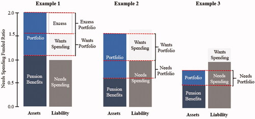
In Figure 2 we see that the potential portfolio allocations vary materially depending the asset and liability composition. The underlying portfolios for the respective liabilities could vary both in terms of the allocation to risky assets (e.g., equities) as well as underlying asset classes (e.g., weights to nominal versus inflation-linked bonds).

This idea of segmenting assets based on the objective is very much related to the growing field of goals-based investing. Thaler (1985) introduced the idea of mental accounting (“buckets”), and Shefrin and Statman (2000) more formally introduced the idea of behavioral portfolio theory. Creating distinct portfolios for each goal may result in strategies that are more behaviorally efficient, something that has been discussed by Brunel (2003), Nevins (2004), and Chhabra (2005), among others, and results in portfolios that are not necessarily any less efficient than strategies employing more traditional methods depending on the evaluation metrics used (Das et al. 2010).

The “matching” aspect of the funded ratio methodology to respective spending goals may be attractive to asset managers who want more targeted individualized portfolios and may be explored further in future research.

Redefining the Optimal Outcome

Retirees clearly have the ability to adjust spending (i.e., portfolio withdrawals) during retirement (i.e., the retirement goal is not entirely inelastic), and we have introduced a model that can dynamically adjust withdrawals and that accounts for varying levels of spending elasticity. Next, we introduce a utility model to more accurately capture the expected satisfaction of accomplishing a retirement goal.

While utility metrics are relatively common in academic research on optimal retirement strategies (e.g., used by Yaari [1965] in his pioneering research on the potential value of annuities) and are far more adaptive than success-related metrics, they are relatively rare in financial planning tools. Utility functions can be somewhat unstable and often do not yield outcomes metrics that would be generally accessible to financial advisors and especially clients, two potential reasons for their general lack of popularity among non-academics.

The most common utility functions in retirement research assume Constant Relative Risk Aversion (CRRA), which is based on the idea of diminishing marginal utility. In this framework, each additional unit of some good (e.g., consumption) is assumed to result in more satisfaction (utility), but at a decreasing rate. This means that retirees want to spend as much as possible, but they must balance the desire to spend more with a potential shortfall, where shortfalls are typically more painful than additional spending.

More complex utility functions distinguish risk aversion in a single period from intertemporal risk aversion by using a recursive utility function described by Epstein and Zin (1989), where volatility in consumption within a given run or assumed lifetime (defined as the elasticity of intertemporal substitution) is considered separately from the volatility of consumption across runs (generally defined as general risk tolerance).

For this research, we use a utility function based on prospect theory, a field introduced by Kahneman and Tversky (1979). Prospect theory suggests that individuals evaluate outcomes based on a specific reference point and that deviations from this value (positive and negative) are valued differently (i.e., losses receive more weight than gains). More specifically, prospect theory suggests that individual utility functions are concave in the domain of gains and convex in the domain of losses.

Our research uses a utility model with three specific ranges, where the utility derived from a given level of spending (i.e., consumption) depends on how that spending relates to the retiree’s total income goal for that respective year. More specifically, the expected utility ($u$) of a given amount of income ($i$) for a given year ($t$) is based on the respective total income goal ($g$).

Total utility is based on the percentage of the overall goal that is defined as a need ($n$), or is nondiscretionary, as well as the assumed income risk aversion level ($\gamma$) for that level income. The risk aversion parameter is based on whether spending is satisfying a needs goal or wants goal, based on Equations (3)(3) $$\mathrm{If}\mathrm{ }\frac{i}{g}\le n\text{ then }{u}_t=\left(\left(\frac{1}{\frac{i_t}{{\left(g\left(n\right)\right)}^{{-\gamma }_n}}}\right)n\right)g$$(3) , (4)(4) $$\mathrm{If}\mathrm{ }\frac{i}{g}>n\text{ and }\frac{i}{g}\le 1\text{ then }{u}_t=\left(\left(g\left(n\right)\right)+\left(\left(\frac{1}{\frac{\left(i_t-\left(g\right(n\left)\right)\right)}{{\left(g-\left(g\right(n\left)\right)\right)}^{{-\gamma }_w}}}\right)\mathrm{*}(1-n)\right)\right)g$$(4) , and (5)(5) $$\mathrm{Else}\mathrm{ }{u}_t=\left(\frac{1}{{\left(\frac{i_t}{g}\right)}^{-{\gamma }_e}}\right)g$$(5) . (3) $$\mathrm{If}\mathrm{ }\frac{i}{g}\le n\text{ then }{u}_t=\left(\left(\frac{1}{\frac{i_t}{{\left(g\left(n\right)\right)}^{{-\gamma }_n}}}\right)n\right)g$$(3) (4) $$\mathrm{If}\mathrm{ }\frac{i}{g}>n\text{ and }\frac{i}{g}\le 1\text{ then }{u}_t=\left(\left(g\left(n\right)\right)+\left(\left(\frac{1}{\frac{\left(i_t-\left(g\right(n\left)\right)\right)}{{\left(g-\left(g\right(n\left)\right)\right)}^{{-\gamma }_w}}}\right)\mathrm{*}(1-n)\right)\right)g$$(4) (5) $$\mathrm{Else}\mathrm{ }{u}_t=\left(\frac{1}{{\left(\frac{i_t}{g}\right)}^{-{\gamma }_e}}\right)g$$(5)

Although the model only assumes two primary types of goals (needs and wants), the model could easily be extended to consider additional types of spending goals (e.g., wishes).

If we assume an income risk aversion levels of 4, 1, and 0.25 for ${\gamma }_n,$ ${\gamma }_w,$ and ${\gamma }_e,$ respectively, we can generate expected utility values for various levels of spending. These are included in Figure 3, where the assumed “need” ($n$) is either 50% or 90% of the total retirement income goal, in Panels A and B, respectively.

Figure 3. Utility of Income for Various Goal Funding and Needs Levels

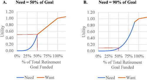
Figure 3 demonstrates that the expected level of utility from a given spending level using this model can vary significantly depending on the composition of a retirement goal (i.e., needs versus wants), even if the same income level is achieved. For example, if we assume the total income goal is $100,000 and the retiree realizes $50,000 (i.e., 50% of the target), the result would be 0.5 units of utility if the need represents 50% of the goal (Panel A) versus only approximately 0.1 units of utility if the need represents 90% of the goal (Panel B).

These differences demonstrate how two retirees with similar total spending goals (and income levels) could have very different retirement funding strategies depending on the composition of their assets and overall funded status. For example, allocating to guaranteed income would generally be more attractive for retirees whose “needs” represent a higher portion of the spending goal to reduce the uncertainty (and associated shortfall), especially for those who do not already have guaranteed income sources (e.g., Social Security retirement benefits) to cover needs spending.

Given the expected utility for a level of spending in a given year ($u_t$), estimated using Equations (3)(3) $$\mathrm{If}\mathrm{ }\frac{i}{g}\le n\text{ then }{u}_t=\left(\left(\frac{1}{\frac{i_t}{{\left(g\left(n\right)\right)}^{{-\gamma }_n}}}\right)n\right)g$$(3) , (4)(4) $$\mathrm{If}\mathrm{ }\frac{i}{g}>n\text{ and }\frac{i}{g}\le 1\text{ then }{u}_t=\left(\left(g\left(n\right)\right)+\left(\left(\frac{1}{\frac{\left(i_t-\left(g\right(n\left)\right)\right)}{{\left(g-\left(g\right(n\left)\right)\right)}^{{-\gamma }_w}}}\right)\mathrm{*}(1-n)\right)\right)g$$(4) , and/or (5)(5) $$\mathrm{Else}\mathrm{ }{u}_t=\left(\frac{1}{{\left(\frac{i_t}{g}\right)}^{-{\gamma }_e}}\right)g$$(5) , we can estimate the constant amount of income with the same utility as the actual income path (ΙΙ). This would be the utility-equivalent constant income level and provides insight into the elasticity of intertemporal substitution. This is given by Equation (6)(6) $$II=\left(\frac{\mathrm{ }\sum _{t=0}^T{\hspace{0.17em}q}_t{\left(1+\rho \right)}^{-t}{u}_t}{\mathrm{ }\sum _{t=0}^T{\hspace{0.17em}q}_t{\left(1+\rho \right)}^{-t}}\right)$$(6) , where $u_t$ is the utility-adjusted income in year $t,$ $q_t$ is the probability of surviving to at least year $t,$ T is the final year of retirement (i.e., the length of the assumed simulation), and $\rho$ is the investor’s subjective real discount rate. (6) $$II=\left(\frac{\mathrm{ }\sum _{t=0}^T{\hspace{0.17em}q}_t{\left(1+\rho \right)}^{-t}{u}_t}{\mathrm{ }\sum _{t=0}^T{\hspace{0.17em}q}_t{\left(1+\rho \right)}^{-t}}\right)$$(6)

To assume a fixed retirement period (e.g., 30 years), a user would set $q_t$ to one and $T$ to the target length of retirement. If a user wanted each year to be considered equally in the calculation, $\rho$ would be set to zero, where the resulting statistic would be a simple average of annual income utility levels.

The overall expected utility of a given strategy is measured using the CRRA utility function with a risk tolerance parameter ($\lambda$) as noted in Equation (7)(7) $$U_t\mathrm{ }={\left[\sum _{i=1}^R{p}_i{\left({II}_i\right)}^{-\lambda }\right]}^{\frac{1}{-\lambda }}$$(7) , where R is the number of paths (or runs), p_i is the probability of path i occurring (which is set to 1/$R,$ i.e., the number of runs), and $U_t$ would be the certainty-equivalent of the stochastic utility-adjusted income $II.$ (7) $$U_t\mathrm{ }={\left[\sum _{i=1}^R{p}_i{\left({II}_i\right)}^{-\lambda }\right]}^{\frac{1}{-\lambda }}$$(7)

When considering multiple strategies (e.g., spending levels, portfolio risk levels, annuity allocations) the optimal strategy would be the one that maximizes $U_t.$

We generate an outcomes metric that should be relatively accessible to investors by dividing the certainty-equivalent utility-adjusted income ($U_t$) by the income goal ($g$), yielding a metric we refer to as the “goal completion score” as noted in Equation (8)(8) $$\mathit{Goal}\mathrm{ }\mathit{Completion}\mathrm{ }\mathit{Score}\mathrm{ }=\mathrm{ }\frac{U_t}{g}$$(8) . (8) $$\mathit{Goal}\mathrm{ }\mathit{Completion}\mathrm{ }\mathit{Score}\mathrm{ }=\mathrm{ }\frac{U_t}{g}$$(8)

This metric provides context around the percentage of the goal completed, adjusted for utility. The goal completion score can be used to convey the overall efficacy of a given strategy to a retiree, that is in the spirit of more common metrics used in financial plans, such as the probability of success (higher is better, with a target of ∼100), but is more holistic in that it considers preferences around spending elasticity.

The utility model developed in this paper is focused on accomplishing a single type of goal. In reality, a household may have multiple financial goals that could differ significantly in terms of timing, size, and scope (e.g., retirement income, bequest, college funding). With respect to this model, each goal should likely be considered separately; however, assets available for funding each goal could be considered jointly, which would require some ordering logic given potential competing priorities. Alternatively, specific accounts could be allocated to fund each goal without overlap. While in theory, all goals could be considered jointly, as a single goal, this utility model is designed for goals that are relatively similar over time. Nevertheless, there are ways to adjust the respective weights if multiple goals are considered, for example, goals based on how the income utility values are weighted and combined.

One additional potential concern with the utility function is that it would generally suggest that underfunded households (i.e., those headed toward ruin) would prefer a riskier portfolio, which may not be practical. This issue is not necessarily unique to this model though. Therefore, while this model is designed to more accurately capture retiree preferences than other more common metrics (e.g., the probability of success), it is not without its weakness.

Analysis

This section provides additional context on the model in a stochastic setting. For our base scenario, we assume the retiree household to be a joint couple, male and female, both aged 65, retiring immediately. The retiree couple has an $80,000 total retirement income goal, that is assumed to increase annually by inflation, of which 70% is classified as being a “need” ($56,000 of the total $80,000 goal).

The retiree couple will receive $40,000 in annual Social Security benefits (which increase with inflation) and will therefore have to generate the remaining $40,000 from $1 million in assumed total retirement savings (i.e., which is consistent with the often-noted “4% Rule”).

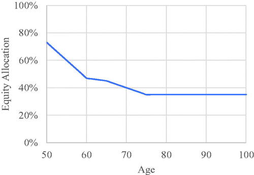
Key model parameters are included in Appendix A and the assumed equity glide path in retirement is included in Appendix B. Figure 4 provides insight into the distribution of income at various percentiles, as well as context around where the respective income level falls across the needs and wants income goals.

Figure 4. Distribution of Simulation Outcomes

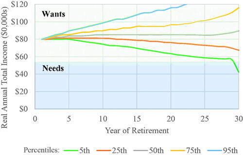
We can see that for the vast majority of runs, the “needs” goal is fully achieved for the entire duration of retirement. Even for the worst one in 20 runs (the fifth percentile) the goal is still accomplished up until the last year of retirement, where the total income generated is $42,263, or 75% of inflation-adjusted needs goal for that year. Note, had the income amount not been adjusted downward throughout the simulation, the portfolio would have been depleted sooner, potentially much sooner based on the trial.

While total spending is expected to decline, in real terms, for approximately 30% of scenarios moving through retirement (with the spending level below the initial $80,000, in today’s dollars), the reductions largely only affect the “wants” spending goal, and in approximately 70% of scenarios total real income is actually expected to increase during retirement. Viewing the continuum of potential retirement outcomes through this lens (i.e., as the distribution of potential income) provides a very different perspective than one using a traditional analysis with a static spending assumption where the outcome is defined based on the probability of success. For example, the probability of success for this simulation is 70.2% (assuming a static real income goal), while the goal completion score is 98.2%.

While a probability of success of 70.2% is not necessarily a bad outcome, it does not convey the same level of (high) certainty as a 98.2% goal completion score. In other words, while the probability of success implies a decent amount of uncertainty regarding the retirement income goal (29.8% probability of failure, or adjustment, depending on one’s perspective), the actual likelihood of the retirees in this scenario not largely accomplishing their retirement income goal, especially the amount they need, is incredibly low.

This model can lead to notable differences in recommendations around factors like safe initial withdrawal rates, optimal portfolio equity allocations, and recommendation to annuities across various household scenarios. We demonstrate this in various panels in Table 2, which are based on an additional set of analyses.

Table 2. Optimal Retirement Strategies Using Goal Completion Score as the Outcomes Metric

		Need % of Goal
		30%	50%	70%	90%
A. Optimal initial withdrawal rate (%)
Pension Income	$10k	4.1	4.0	4.0	3.8
	$30k	4.5	4.4	4.2	3.9
	$50k	5.1	4.8	4.6	4.0
	$70k	5.4	5.3	5.0	4.0
	$90k	5.3	5.4	5.4	4.0
B. Optimal portfolio static equity allocation (%)
Pension Income	$10k	50	40	40	25
	$30k	55	55	45	35
	$50k	65	60	45	40
	$70k	70	65	50	40
	$90k	75	75	55	45
C. Optimal annuity allocation (%)
Pension Income	$10k	50	50	50	50
	$30k	25	30	35	40
	$50k	10	15	30	30
	$70k	0	0	15	25
	$90k	0	0	5	10

In Panel A, we solve for the initial withdrawal rate that yields a 95% goal completion score³ for various scenarios. In Panel B, we solve for the optimal portfolio equity allocation, assuming a 5% initial withdrawal rate. In Panel C, we solve for the optimal allocation to an immediate annuity, assuming a 5% initial withdrawal rate and a nominal annuity payout rate of 4.75% (with a maximum potential allocation of 50%).

As a reminder, if the outcomes metric is the probability of success, then the percentage of the goal that is defined as needs and the relative amount of guaranteed income (holding the portfolio value constant) has no impact on optimal initial withdrawal rates, equity allocation, or annuity allocations, especially if taxes are ignored. In other words, the values in Panels A, B, and C should not vary if the probability of success is the outcomes metric. This is because the probability of success focuses entirely on the marginal role of the portfolio when it comes to funding the liability and does not consider magnitude of failure (or allow for dynamic adjustments). The results in Table 2, though, clearly demonstrate that a more nuanced perspective of household assets and preferences can have a significant impact on optimal retirement strategies if appropriately considered.

For example, in Table 2, optimal initial withdrawal rates (Panel A) and equity allocations (Panel B) are highest for retirees who have higher levels of guaranteed income and more elasticity with respect to retirement spending, while annuity allocations (Panel C) are highest for retirees who have lower levels of guaranteed income and less elasticity with respect to retirement spending using this model.

The differences in Table 2 can have notable implications for things like required retirement savings. For example, focusing on withdrawal rates (Panel A), an initial withdrawal rate of 3.8% (low pension income and high needs goal) effectively requires 36.8% more savings than an initial withdrawal rate of 5.2% (high pension income and low needs goal). This is a staggering difference. Alternatively, the higher withdrawal rate implies the household could spend significantly more in retirement. Additionally, the potential benefit of allocating to an annuity (Panel C) varies, whereby retirees who already have high levels of guaranteed income and a relatively flexible spending goal clearly benefit less from annuitization.

Overall, the results of this section suggest that using the retirement income models introduced in this piece, which incorporate dynamic withdrawals and spending elasticity and can account for expected utility across income levels, can lead to notably different retirement recommendations for retirees, especially when compared to outputs generated from probability of success-related metrics.

Conclusions

Despite significant advances in computing power and a relatively extensive body of research on the nature of retirement, assumptions in retirement research and income planning tools have evolved only modestly over the last 30 years. This lack of evolution has created an environment where many financial advisors and online calculators provide overly simplistic advice on one of the most important (and expensive) decisions made by households: how much they need to save for retirement (and can spend during it).

This research builds off of decades of existing literature in the retirement income space and introduces a series of models that can improve retirement income projections by better understanding the elasticity of spending, modeling changes in spending based on changes in finances, and determining the optimal strategy using a utility function that better quantifies the expected satisfaction across outcomes. While there are a number of other existing approaches similar to those introduced in this research, most of these approaches are relatively narrowly focused and cannot easily be used to generate a more comprehensive perspective on retirement modeling. This research is unique in introducing models specifically designed to work together that be easily configured and allow for a variety of client scenarios and user assumptions.

There are a number of potential extensions associated with this research, such as extending the model to include additional goals (e.g., wishes), determining optimal portfolio allocations for the different types of “mapped” goals (e.g., needs and wants), determining the optimal parameters to use with the funded ratio dynamic spending rule, as well as exploring the more general parameters in the model.

In closing, given the significant time and energy associated with funding retirement, it is important that the estimate be as accurate as possible. This research demonstrates that existing retirement planning frameworks (and tools) have notable deficiencies that should be addressed to ensure retirees (and savers) receive the best guidance and advice possible.

Disclosure Statement

PGIM DC Solutions is currently developing a series of solutions based on this research and methodologies.

Additional information

Notes on contributors

David Blanchett

David Blanchett, CFA, is the head of Retirement Research, PGIM DC Solutions, Newark, NJ.

Notes

1 Other notable research includes Milevsky, Ho, and Robinson (1997) and Cooley, Hubbard, and Waltz (1998).

2 https://www.bls.gov/cex/pumd.htm

3 This is a subjective target and can obviously vary by user or client.

Appendices

Appendix A. Modeling Assumptions

Table

Assumption Regarding	Variable	Value
Income goal	$g$	$80,000 (varies)
% of goal that is need	$n$	70% (varies)
Risk aversion factor for needs spending	${\gamma }_n$	4
Risk aversion factor for wants spending	${\gamma }_w$	1
Risk aversion factor for excess spending	${\gamma }_e$	0.25
Length of projection/end of retirement	$T$	30
Number of simulation runs/trials	$R$	1,000
Probability of survival	$q_t$	1 (fixed retirement period)
Discount rate for EOIS calculation	$\rho$	0
Risk aversion factor for certainty-equivalent	$\lambda$	2
Nominal discount rate for needs spending	$r_n$	5%
Nominal discount rate for wants spending	$r_w$	4%
Nominal discount rate for inflows (guaranteed income)	$r_p$	3%
Inflation		2%
Equity, annual arithmetic return		7.5%
Equity annual standard deviation		20%
Bonds, annual arithmetic return		2.5%
Bonds, annual standard deviation		5%
Stock/bond correlation		0.0
Taxes are ignored for the analysis

EOIS = Elasticity of intertemporal substitution.

 

Appendix B. Equity Glide Path

References

- Bengen, William. 1994. “Determining Withdrawal Rates Using Historical Data.” Journal of Financial Planning 7 (4): 171–80.
- Bengen, William. 2001. “Conserving Client Portfolios during Retirement, Part IV.” Journal of Financial Planning 14 (5): 110–9.
- Blanchett, David, and Larry Frank. 2009. “A Dynamic and Adaptive Approach to Distribution Planning and Monitoring.” Journal of Financial Planning 22 (4): 52–66.
- Brunel, Jean. 2003. “Revisiting the Asset Allocation Challenge through a Behavioral Finance Lens.” The Journal of Wealth Management 6 (2): 10–20. doi:10.3905/jwm.2003.320479.
- Chhabra, Ashvin. 2005. “Beyond Markowitz: A Comprehensive Wealth Allocation Framework for Individuals.” The Journal of Wealth Management 7 (4): 8–34. doi:10.3905/jwm.2005.470606.
- Cooley, Phillip, Carl Hubbard, and Daniel Waltz. 1998. “Retirement Spending: Choosing a Sustainable Withdrawal Rate.” Journal of the American Association of Individual Investors 20 (2): 16–21.
- Das, Sanjiv, Harry Markowitz, Jonathan Scheid, and Meir Statman. 2010. “Portfolio Optimization with Mental Accounts.” Journal of Financial and Quantitative Analysis 45 (2): 311–34. doi:10.1017/S0022109010000141.
- Epstein, Larry G., and Stanley E. Zin. 1989. “Substitution Risk Aversion and the Temporal Behavior of Consumption and Asset Returns: A Theoretical Framework.” Econometrica 57 (4): 937–69. doi:10.2307/1913778.
- Finke, Michael, Wade D. Pfau, and David M. Blanchett. 2013. “The 4 Percent Rule Is Not Safe in a Low-Yield World.” Journal of Financial Planning 26 (6): 46–55. https://www.financialplanningassociation.org/article/4-percent-rule-not-safe-low-yield-world
- Guyton, Jonathan. 2004. “Decision Rules and Portfolio Management for Retirees: Is the ‘Safe’ Initial Withdrawal Rate Too Safe?” Journal of Financial Planning 17 (10): 54–62.
- Habib, Faisal, Huaxiong Huang, and Moshe Milevsky. 2017. “Approximate Solutions to Retirement Spending Problems and the Optimality of Ruin.” Working paper, version March 31 2017.
- Idzorek, Thomas, and David Blanchett. 2019. “LDI for Individual Portfolios.” The Journal of Investing 28 (1): 31–54. doi:10.3905/joi.2019.28.1.031.
- Kahneman, Daniel, and Amos Tversky. 1979. “Prospect Theory: An Analysis of Decision under Risk.” Econometrica 47 (2): 263–91. doi:10.2307/1914185.
- Kaplan, Paul, and David Blanchett. 2021. “A Dynamic Spending Rule for All Retirees.” Working Paper.
- Merton, Robert. 1969. “Lifetime Portfolio Selection under Uncertainty: The Continuous-Time Case.” The Review of Economics and Statistics 51 (3): 247–57. doi:10.2307/1926560.
- Milevsky, Moshe, Kwok Ho, and Chris Robinson. 1997. “Asset Allocation via the Conditional First Exit Time or How to Avoid Outliving Your Money.” Review of Quantitative Finance and Accounting 9 (1): 53–70. doi:10.1023/A:1008278910581.
- Milevsky, Moshe, and Huaxiong Huang. 2011. “Spending Retirement on Planet Vulcan: The Impact of Longevity Risk Aversion on Optimal Withdrawal Rates.” Financial Analysts Journal 67 (2): 45–58. doi:10.2469/faj.v67.n2.2.
- Nevins, D. 2004. “Goals-Based Investing: Integrating Traditional and Behavioral Finance” Journal of Wealth Management 6 (4): 8–23. doi:10.3905/jwm.2004.391053.
- Pfau, Wade. 2010. “An International Perspective on Safe Withdrawal Rates from Retirement Savings: The Demise of the 4 Percent Rule?” Journal of Financial Planning 23 (12): 52–61.
- Pye, Gordon. 2001. “Adjusting Withdrawal Rates for Taxes and Expenses.” Journal of Financial Planning 14 (4): 126–36.
- Rubinstein, Mark. 1976. “The Strong Case for the Generalized Logarithmic Utility Model as the Premier Model of Financial Markets.” The Journal of Finance 31 (2): 551–71. doi:10.2307/2326626.
- Shefrin, Hersh, and Meir Statman. 2000. “Behavioral Portfolio Theory.” The Journal of Financial and Quantitative Analysis 35 (2): 127–51. doi:10.2307/2676187.
- Stout, Gene, and John Mitchell. 2006. “Dynamic Retirement Withdrawal Planning.” Financial Services Review 15:117–31.
- Thaler, Richard. 1985. “Mental Accounting and Consumer Choice.” Marketing Science 4 (3): 199–214. doi:10.1287/mksc.4.3.199.
- Waring, Barton, and Laurence Siegel. 2015. “The Only Spending Rule You Will Ever Need.” Financial Analysts Journal 71 (1): 91–107. doi:10.2469/faj.v71.n1.2.
- Waring, Barton, and Laurence Siegel. 2018. “What Investment Risk Means to You, Illustrated: Strategic Asset Allocation, the Budget Constraint, and the Volatility of Spending during Retirement.” The Journal of Retirement 6 (2): 7–26. doi:10.3905/jor.2018.1.041.
- Yaari, Menahem. 1965. “Uncertain Lifetime, Life Insurance, and the Theory of the Consumer.” The Review of Economic Studies 32 (2): 137–50. doi:10.2307/2296058.