Targeting Macroeconomic Exposures in Equity Portfolios: A Firm-Level Measurement Approach for Out-of-Sample Robustness

Abstract

We propose firm-level measures of exposures to macroeconomic risks that substantially improve out-of-sample robustness compared to standard estimation approaches. Systematic equity strategies constructed from such measures offer more consistent macro exposures out of sample than strategies that allocate across sectors or equity-style factors. We do not find significant cost to the performance of such systematic strategies in exchange for targeting exposures to macroeconomic risks, such as interest rates, term spread, credit spread, or inflation. Our methodology can be used to construct equity portfolios for investors who have hedging demands or active views regarding macroeconomic conditions.

Keywords:

• macroeconomic risks
• out-of-sample exposure
• systematic equity strategies

PL Credits: 2.0:

Introduction

This paper proposes a method of targeting exposures to macroeconomic risks in equity investing. Managing macroeconomic risks is an important task for equity investors because their portfolios may come with substantial exposures to not only stock market risk but also broader macroeconomic risks, such as interest rate risk, inflation risk, or recession risk.

Beyond the exposure that the broad market index may have to such macroeconomic factors, investors may pick up cross-sectional differences in exposure. There is ample evidence that such differences in stocks’ macro exposures can be substantial. For example, Chen, Roll, and Ross (1986) found that portfolios sorted on market-capitalisation had different exposures to various macroeconomic variables, including the term spread and the credit spread. Similar findings were documented by Petkova (2006) across double-sorted portfolios on book-to-price and market capitalisation and by Boons (2016) across stock-level returns. Such implicit exposures will not necessarily align with what an investor would target when considering macroeconomic risk exposures explicitly. If an investor is already exposed to a given macroeconomic risk outside their equity allocation, the total portfolio will not be well diversified and suffer losses if a given macroeconomic risk materialises. For example, an increase in credit spreads often signals a slowdown in economic activity and a negative impact on labour income. Investors who take above-average exposure to credit risk in their equity portfolios might load up on exposure they already have through their labour income. Similarly, the liabilities of an investor increase with declining interest rates. Investors with liabilities thus should consider how their equity portfolio reacts to changes in interest rates.

In practice, managing macro risks is often done via allocation across asset classes. There are various studies that focus on constructing mimicking portfolios of different economic variables through dynamic asset allocation (see, e.g., Jurczenko and Teiletche 2020 and Swade et al. 2021). In contrast, this paper focusses on a single asset class. Focussing on equity portfolios poses challenges because exposure to macroeconomic risks may be less diverse and more difficult to measure. However, investors may have preference to manage macroeconomic risks in equities for different reasons. For example, equities have delivered the largest premium historically amongst traditional asset classes. Investors could be better off if they can achieve their macro risk objectives whilst collecting the long-term equity premium, especially during the times when compensation for other asset classes, such as long-term bonds or inflation-protected securities, are at historical lows.

In a related paper, Chousakos and Giamouridis (2020) assess the premia in equity markets associated with macro risks, such as growth, fragility, and volatility. Whilst their paper focusses on pricing and performance enhancements from new types of macro factors, our paper focusses on measurement of exposures and robustness out of sample to long-established macro-state variables.

A better understanding of how to measure exposures reliably is valuable for investors. Reliable measurement of how different stocks are exposed to macroeconomic risks would allow investors to build equity portfolios that hedge undesired macro risks. In addition, targeting macroeconomic exposures is useful for investors who have views on the future economic conditions.

However, this is easier said than done. One of the major challenges to efficiently managing macro risks in equity portfolios is to reliably estimate the exposures. Most academic studies are concerned with ex-post analysis over the long term. Common estimation techniques available in the literature do not consider out-of-sample reliability. For example, one of the earliest influential studies on this subject by Chen, Roll, and Ross (1986) applied the ordinary least-squares (OLS) approach to monthly returns to obtain betas to different macroeconomic variables, such as inflation, growth, term spread, and credit spread. Bali, Brown, and Caglayan (2014) used monthly estimates of macroeconomic uncertainty to measure firm-level exposures using OLS regression. Levi and Welch (2017) find that roughly two-thirds of the papers published in the top academic finance journals between 2013 and 2015 estimate betas using a monthly frequency over samples of 1 to 5 years.¹ Whilst the use of simple estimation procedures is suitable for ex-post analysis of investment strategies, the reliability of out-of-sample exposures is the key concern when investors’ objective is to target these macro exposures in their portfolios.

The empirical evidence shows that estimating the relation between equities and macroeconomic variables is hard. Ang, Brière, and Signori (2012) authored one of the few studies specifically focussing on the out-of-sample reliability of macro betas. They find that a portfolio of stocks with high inflation betas over the recent past has inflation betas that are indistinguishable from zero out of sample. Fama and French (1997) emphasise that exposures of industry portfolios to equity risk factors are measured with a high margin of error. Boons (2016) acknowledges that estimating exposures to macroeconomic variables is difficult and proposes various statistical adjustment to achieve out-of-sample reliability.² In general, naïve estimation techniques that are common in academic studies, such as standard regression betas estimated on a low frequency, are not suitable for out-of-sample measurement of risk exposures.

In light of the difficult measurement of macro exposures, investment decisions in practice are often discretionary. For example, some actively managed funds explicitly aim at strong outperformance in high inflationary periods. However, discretionary choices to target macro exposures are hard to evaluate given their lack of transparency and replicability.

To target macro exposures of equity portfolios, the approach of choice in investment practice is to allocate across predefined asset classes, such as sectors or factors. However, whilst such building blocks are readily available, they have never been designed to reliably capture macro risks. Using such blunt tools may in fact compound the measurement challenges when trying to target macro exposures.

In contrast to popular practice, we propose a systematic approach that is transparent and replicable. We also go beyond analysing sector differences and instead exploit the firm-level heterogeneity of risk exposures. Our approach relies on three ingredients.

First, we choose forward-looking macroeconomic variables that are derived from financial markets. This allows us to identify links between stock-level returns and macroeconomic risks. Commonly used macroeconomic variables, such as realised inflation or growth, are backward looking and do not reflect investor expectations. They also come at a lower frequency that aggravates the challenge of exposure measurement. Our macroeconomic variables are derived from asset prices, such as fixed-income securities. They are available at higher frequency and naturally incorporate investor expectations, thus improving the reliability of exposure measurement.

Second, we apply robust measurement tools to estimate stock-level macro exposures out of sample. Our estimation technique is superior to the naïve approach that uses OLS on data that come at a relatively lower frequency.

Third, we construct dedicated equity portfolios from stock-level exposures in a fully systematic way. We show that our stylised strategies can provide stronger out-of-sample macro exposures than other popular approaches in the industry that allocate across preexisting equity products, such as sector or factor indices. This finding is consistent across all the macro variables that we test.

In addition to capturing macroeconomic exposures in a reliable fashion, our stylised strategies come with performance in line with market returns, irrespective of the macroeconomic risks they target. Therefore, such strategies provide access to the long-term equity premium along with targeting the macroeconomic risks that an investor might be concerned with.³

Selecting Forward-Looking Variables

In general, realised quantities of fundamental economic measures are not suited when analysing movements in asset prices. In liquid markets, information is quickly reflected in prices. Prices of financial assets that are claims to future cash flows depend on investors’ expectations. Therefore, looking at realised measures of economic variables that lack information about future economic conditions does not allow to capture the relation between asset prices and economic conditions. Instead, we rely on macro-state variables that are forward looking and quickly incorporate available information. For example, if investors’ expectations about future interest rates change, this information is reflected in asset prices, in particular treasury bond prices. Similarly, the aggregate credit spread reflects investors’ risk tolerance and whether future economic conditions are expected to alter firms’ ability to meet their obligations.

We primarily rely on U.S. data. However, our approach can be easily extended to other geographical areas where the respective macro variables are available. Below, we list the macro variables that we use in our analysis:⁴

1. Short-term interest rates, defined as a yield on 3-month U.S. Treasury bills.

2. Term spread, defined as a difference between yields on 10-year and 1-year U.S. Treasury bonds.

3. Credit spread, defined as a difference between yields on Moody’s Corporate Baa and Aaa bonds.

4. Expected inflation, defined as a difference between the yields of nominal 10-year Treasury bonds and 10-year Treasury Inflation Protected Securities (TIPS).

Note that all four macro variables are derived from asset prices and thus reflect investors’ perception on economic conditions. Amenc et al. (2019) provide a protocol for selecting relevant state variables and show that such variables⁵ are useful in predicting aggregate economic conditions and provide information on the aggregate risk tolerance of investors.⁶

Short-term interest rates are highly influenced by monetary policy actions, and they are also considered as a proxy for the risk-free rate. Surprises in short rates not only reflect central bank actions but also reflect the demand on safe assets in a “flight to quality” (Longstaff 2004). The term spread is one of the most often used macro variables to forecast economic growth and recessions (Campbell 1987; Estrella and Trubin 2006). It is also considered a general measure of compensation for exposure to shocks on long-term discount rates.⁷ The default spread signals risk aversion during adverse economic conditions, when equity and bond investors require higher compensation for bearing risk. Fama and French (1989) and Keim and Stambaugh (1986) provide empirical evidence for such a link. Finally, expected inflation determines the purchasing power of future cash flows. It therefore has a direct impact on asset prices, especially those that produce cash flows adjusted for inflation (such as TIPS). The four state variables provide information about aggregate expectations about different dimensions of economic conditions.

Also note that our macro-state variables are available at high frequency, which is not the case for backward-looking economic fundamental measures, such as realised inflation or growth. High-frequency data are beneficial in statistical estimation procedures, as we will discuss in detail later in this section.

Surprises Matter, Not Levels

Another important aspect of our methodology is to use surprises, or innovations, in macro variables instead of levels. The current value of assets already reflects information that is known to investors today. As new information arrives, asset prices, including stock prices, adjust accordingly. Therefore, we are interested in surprises. In fact, the observed level of a macroeconomic variable that was fully anticipated by investors will not lead to different price reactions across stocks.

Consider the example of surprises in expected inflation. In Figure 1, we plot the levels as well as innovations in breakeven inflation over a selected period around the 2008/2009 global financial crisis. More specifically, we consider a period from 2006 to 2012. Looking at the level of breakeven inflation, we see that in December 2008, breakeven inflation is very low (close to zero). From December 2008 to July 2009, inflation rises strongly to about 1.7% but remains at levels that are far below earlier levels of about 2.5%. In the first half of 2009, inflation levels were low but innovations in breakeven inflation were actually high, as the U.S. economy rebounded from the financial crisis.

Figure 1. Innovations in Macro Variables Are Different from Levels: The Case of Breakeven Inflation

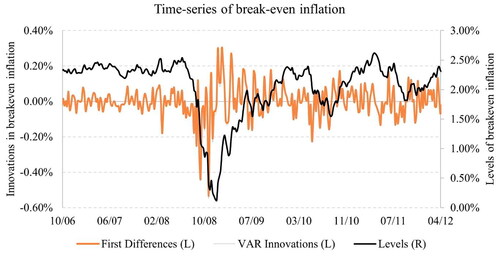
Now consider a stock which benefits from high levels of inflation and suffers when they are low. During the first half of 2009, all else being equal, you would expect such a stock to achieve positive performance because markets would be likely to reprice it whilst moving from a very low inflation environment to one of moderate inflation (though the price of such a stock might still be below its prior value, as inflation was much higher at 2.5% before 2008). Still, the inflation sensitivity of such a stock will show up in price movements over the short term. To pick up the sensitivity of stock returns with inflation, we need to look at the contemporaneous changes in breakeven inflation that were not anticipated by investors, rather than looking at the level of inflation. Of course, this argument also applies to other macro variables, such as the term spread, credit spread, and interest rates.

In general, the current value of assets already reflects information that is known to investors, such as the current values of macro variables. As new information arrives, stock prices will adjust accordingly.

When it comes to estimating anticipated changes in a macroeconomic variable, there are various methods available. The standard approach followed in literature is to use a vector auto-regressive model (VAR). In our case, we can simply use the change of macro variables as it delivers similar results to a more involved model, such as a VAR model.⁸ As shown in Figure 1, the VAR innovations are not distinguishable from simple first-order differences in breakeven inflation. We find a similar picture when looking at other macro variables.

Statistical Estimates of Macro Exposures

We now describe the necessary ingredients for robust estimates of macro exposures. Our objective is to exploit differences in stock-level macro exposures without altering access to the market premium. Therefore, we control for the market exposure when we estimate stock-level macro exposures. We start from a simple bivariate linear model: (1) $${\mathit{R}}_{\mathit{i},\mathrm{ }\mathit{t}}-{\mathit{R}}_{\mathit{RF},\mathrm{ }\mathit{t}}={\mathit{\alpha }}_{\mathit{i}}+{\mathit{\beta }}_{\mathit{i}}^{\mathit{MKT}}\left({\mathit{R}}_{\mathit{MKT},\mathrm{ }\mathit{t}}-{\mathit{R}}_{\mathit{RF},\mathrm{ }\mathit{t}}\right)+{\mathit{\beta }}_{\mathit{i}}^{\mathit{macro}}\left({\mathit{Macro}}_{\mathrm{ }\mathit{t}}-{\mathbf{E}(\mathit{Macro}}_{\mathrm{ }\mathit{t}|\mathit{t}-1})\right)+{\mathit{\epsilon }}_{\mathit{i},\mathrm{ }\mathit{t}}$$(1)

The first independent variable corresponds to the equity market premium and the second to innovations in the relevant macro variable. In addition, we take several important steps to ensure that exposures estimated on past data stay reliable out of sample.

First, we use observations at weekly frequency. The data that we rely on are also available at daily frequency, but we use weekly observations to avoid problems due to differences in closing times between bond and equity markets. Levi and Welch (2017) show that using such higher-frequency data provides substantial improvements in accuracy of estimated betas over using monthly returns data. Having higher frequency leads to more observations, which helps to reduce estimation error. This is, however, very uncommon in the literature, especially when working with macro variables (see Levi and Welch 2017).

Second, we manage to account for recent dynamics in macro betas whilst maintaining deep historical samples for estimation. Estimation problems face a basic trade-off between sample size and reactivity to changes in exposures. Using historical data that are a decade old provides a large sample but does not seem ideal as the given firm might have drastically changed over this period. On the other hand, relying on a short window of estimation, such as only the most recent year, will lead to imprecise estimates due to small sample size. We overcome this trade-off by a using long-term history of stock-level returns (20 years if available) and attributing decreasing importance to observations as we go further back in history.⁹ Our methodology differs from commonly used rolling-window approaches in investment practice because we fit the model using the weighted-least squares method. (2) $$\mathit{min}\left\{{\sum }_{\mathit{t}=1}^{\mathit{T}}{{{\mathit{\epsilon }}_{\mathit{t}}}^2\times \mathit{e}}^{-\left|\mathit{T}-\mathit{t}\right|\frac{\mathrm{ }\mathit{ln}\left(2\right)}{260}\mathrm{ }}\right\}$$(2)

The term $\frac{\mathit{ }\mathit{ln}\left(2\right)}{260}$ specifies that, as T approaches infinity, half of the total weights are attributed to the first 260 weeks (i.e., 5 years). Our estimation approach benefits from a large sample whilst also capturing the recent dynamics of macro exposures.

Third, we explicitly account for estimation risk at the firm level. Treating macro exposures of identical magnitude for two stocks as equal would ignore estimation risk. Even if macro betas for two stocks are estimated to be identical in magnitude, they may differ in terms of the uncertainty around the point estimate. Therefore, we also account for the differences in uncertainty across stocks and adjust macro exposures that are estimated imprecisely. Vasicek (1973) proposes Bayesian shrinkage to improve the accuracy of beta estimates. The idea behind this adjustment is to shrink estimated coefficients to a prior. We choose the cross-sectional average exposure estimates as a prior, which is close to 0 most of the time as we control for the market beta in the model. The intensity of shrinkage towards the prior will depend on the magnitude of estimation error for a respective beta estimate. (3) $${\mathit{\beta }}_{\mathit{i}}^{\mathit{final}}={\mathit{\beta }}_{\mathit{i}}^{\mathit{prior}}\frac{{\mathit{\sigma }}_{\mathit{i},\mathrm{ }\mathit{TS}}^2}{{\mathit{\sigma }}_{\mathit{i},\mathrm{ }\mathit{TS}}^2+{\mathit{\sigma }}_{\mathit{XS}}^2}+{\mathit{\beta }}_{\mathit{i}}^{\mathit{estimate}}\left(1-\frac{{\mathit{\sigma }}_{\mathit{i},\mathrm{ }\mathit{TS}}^2}{{\mathit{\sigma }}_{\mathit{i},\mathrm{ }\mathit{TS}}^2+{\mathit{\sigma }}_{\mathit{XS}}^2}\right)$$(3) where by TS we refer to sampling variance and by XS we refer to the cross-sectional variance across estimated beta coefficients.

The final estimate¹⁰ is the weighted average of prior beta and estimated beta. The higher the estimation error, the more importance is given to the prior, and vice versa.

We can summarise the estimation process in three steps:

• The first key ingredient of our methodology is to use surprises in forward-looking variables.

• Second, we employ various statistical adjustments to generate robust estimates of stock-level macro exposures.

• Third, we use the estimated stock-level macro exposures to create dedicated building blocks instead of allocating across existing portfolios (such as sector or factor portfolios).

In the following section, we analyse how our estimation approach performs in terms of out-of-sample reliability and how it compares with alternative approaches.

Assessing the Reliability of Macro Exposures Estimates

We evaluate the reliability of macro exposure estimates by constructing mimicking portfolios. For each macro variable, we create a long-short portfolio that buys stocks with the highest macro exposure estimates (top 30%) and sells stocks with the lowest macro exposures estimates (bottom 30%). The equal-weighted long-short portfolio is formed each quarter and held until the next quarterly rebalancing. The estimation is only based on data available at the rebalancing date, and the realised macro exposures are computed over the holding period. Because the macro mimicking portfolio buys stocks with high exposure and sells stocks with low exposure, we expect that the mimicking portfolio will demonstrate positive realised macro exposure when we go out of sample. If that is the case, we can conclude that ex-ante macro exposure estimates are reliable (and stocks in long leg have higher out-of-sample exposures than stocks in the short leg).

Our analysis starts in June 1970 and spans over 52 years, ending in June 2022. The equity universe consists of the largest 500 stocks in CRSP universe¹¹ and is reviewed each quarter on the third Friday of March, June, September, and December. We focus on the United States, which represents a significant share of global equity markets in terms of market capitalisation. The data for U.S. macro variables cover a long history, whilst data for other developed countries cover substantially shorter periods.¹²

The data for breakeven inflation start only in January 1997. Therefore, when evaluating portfolios that mimic changes in breakeven inflation, we start the analysis in March 2002 because we require at least 5 years of data for estimation of macro exposure. It is possible to create an inflation proxy that also covers the earlier sample period and thus allows for long-term analysis. In particular, we created an economic tracking portfolio that invests in broad asset classes to mimic surprises in breakeven inflation. We find that the conclusions of our analysis remain intact when using such an inflation proxy over a long-term period.¹³

The macro exposures are estimated in a bivariate model that includes the market factor and the corresponding macro factor (see equation 1(1) $${\mathit{R}}_{\mathit{i},\mathrm{ }\mathit{t}}-{\mathit{R}}_{\mathit{RF},\mathrm{ }\mathit{t}}={\mathit{\alpha }}_{\mathit{i}}+{\mathit{\beta }}_{\mathit{i}}^{\mathit{MKT}}\left({\mathit{R}}_{\mathit{MKT},\mathrm{ }\mathit{t}}-{\mathit{R}}_{\mathit{RF},\mathrm{ }\mathit{t}}\right)+{\mathit{\beta }}_{\mathit{i}}^{\mathit{macro}}\left({\mathit{Macro}}_{\mathrm{ }\mathit{t}}-{\mathbf{E}(\mathit{Macro}}_{\mathrm{ }\mathit{t}|\mathit{t}-1})\right)+{\mathit{\epsilon }}_{\mathit{i},\mathrm{ }\mathit{t}}$$(1) ). We estimate realised exposures using standard OLS as our aim is not to produce out-of-sample reliable estimates, but to observe what happens ex-post, over the long-term period.

Before evaluating whether our approach allows creating mimicking portfolios with the desired exposure out of sample, we briefly test mimicking portfolios to backward-looking variables that are commonly used when analysing the sensitivity of equity returns to economic conditions. More specifically, we look at economic growth proxied by industrial production index, as it is available at a monthly frequency (unlike other measures, such as GDP, which is available at a quarterly frequency). For example, Chen, Roll, and Ross (1986) use industrial production growth as one of the factors in their asset pricing model. Ung and Luk (2016) look at the realised growth in GDP to measure sensitivity of different equity-style factors to economic conditions. Devarajan et al. (2016) also propose using GDP growth to measure the cyclical variation of equity factors.

We also look at inflation, proxied by realised changes in the consumer price index. We apply a naïve estimation approach that uses 5 years of recent data at a monthly frequency to estimate stock-level betas to a given macro variable.

Indeed, whilst economic growth and realised inflation are key forces describing macroeconomic conditions, asset prices would typically lead and reflect information about growth and inflation before it is observable through the respective measures (see Fama, 1981). This is one of the reasons that the relation between asset returns and economic variables is often found to be weak.

The results in Table 1 show that exposure estimates to backward-looking variables are unreliable, confirming earlier results on inflation betas of Ang, Brière, and Signori (2012). The realised exposures of mimicking portfolios to these variables are not distinguishable from zero.

Table 1. Out-of-Sample Exposures of Mimicking Portfolios to Backward-Looking Variables

United States 30 June 1970–30 June 2022	Realised Macro Beta	t-Statistic
Mimicking portfolios to backward-looking variables using naïve estimation techniques
Industrial Production Growth	−0.01	−0.28
Consumer Price Index Growth (CPI)	0.23	0.97

Notes: The realised macro exposures are estimated in a bivariate regression that includes the market factor and the corresponding macro variable. Standard errors are adjusted for heteroskedasticity and autocorrelation following Newey and West (1987). We follow Andrews (1991) when determining data-dependent bandwidth/lag truncation parameters, which are estimated in a first-order autoregressive model (AR(1)) with a maximum likelihood method. Statistical significance is indicated by a single asterisk (*) for results that are significant on a 5% basis and double asterisks (**) for results that are significant on a 1% basis.

This analysis illustrates that drawing on commonly used variables and estimation techniques is not suitable for measuring macro exposures. Using backward-looking variables does not support robust estimation of firms’ sensitivity to economic conditions. Even though economic growth and inflation could be important drivers of asset prices, backward-looking information on these dimensions is unlikely to be relevant for stock returns. Choosing the right proxy is essential to establish the link between asset prices and economic fundamentals.

We now move to analysing mimicking portfolios that rely on different exposure measures to forward-looking variables. Table 2 shows realised macro exposures as well as the corresponding t-statistics adjusted for heteroscedasticity and autocorrelation. The exposures are reported for different mimicking portfolios that rely on different estimation techniques.

Table 2. Reliability of Macro Beta Estimates Using Different Regression Specifications: Out-of-Sample Betas with Targeted Macro Variables

Estimation Frequency	Estimation Method	Bayesian Shrinkage	Short Rates	Term Spread	Credit Spread	Breakeven Inflation	Average
Monthly	OLS	No	1.07**	1.20*	1.84	2.73*	1.71
			(4.08)	(2.56)	(1.44)	(2.04)	(2.53)
Weekly	OLS	No	0.83**	1.25**	2.16**	5.37**	2.40
			(5.23)	(4.33)	(3.90)	(3.23)	(4.17)
Weekly	WLS	No	0.83**	1.34**	2.21**	5.32**	2.43
			(5.62)	(4.51)	(3.98)	(3.36)	(4.37)
Weekly	WLS	Yes	0.81**	1.34**	2.28**	5.36**	2.45
			(5.49)	(4.49)	(4.12)	(3.45)	(4.39)

OLS: ordinary least-squares; WLS: weighted least-squares.

Notes: The analysis has been done from 19 June 1970 to 30 June 2022. The only exception is breakeven inflation, for which the analysis starts in 31 March 2002. The out-of-sample macro exposures are estimated in a bivariate regression that includes the market factor and innovations in corresponding macro variable. The estimation frequency and frequency when calculating realised exposures are the same. Standard errors are adjusted for heteroskedasticity and autocorrelation following Newey and West (1987). We follow Andrews (1991) when determining data-dependent bandwidth/lag truncation parameters, which are estimated in a first-order autoregressive model (AR(1)) with a maximum likelihood method. Statistical significance is indicated by a single asterisk (*) for results that are significant on a 5% basis and double asterisks (**) for results that are significant on a 1% basis.

In the first row, we show realised macro exposures for mimicking portfolios that use naïve estimation techniques. More specifically, macro betas are estimated on a monthly frequency over the recent 5 years, using the OLS method. As noted by Levi and Welch (2017), this naïve estimation approach is commonly used in academic studies. The results suggest that some portfolios created using naïve estimation do not come with statistically significant exposures out of sample. In particular, the mimicking portfolio for the credit spread comes with out-of-sample exposure that is far from being statistically significant, with a t-statistic of only 1.44. However, the realised exposures to all variables are positive and more reliable than the exposures we obtained when using the naïve estimation approach to estimate exposure to backward-looking variables. This confirms that our macroeconomic variables contain more relevant information than backward-looking variables, such as the growth and realised inflation.

The second row of Table 2 shows the results when using weekly returns for estimation, but without any further adjustments, such as dynamic weights or Bayesian shrinkage. Therefore, the only difference with the naïve approach is the frequency at which the macro betas are estimated. The realised exposures of macro mimicking portfolios that use weekly returns are much stronger. We see positive and highly significant realised exposures for all macro variables. On average, we observe that realised macro betas increase from 1.71 when using a monthly estimation frequency to 2.40 when using a weekly frequency. Moreover, the t-statistics increase from 2.53 to 4.17 on average. This increase is substantial and clearly indicates that estimating exposures using a weekly frequency is superior to using a monthly frequency.

The third row shows the results obtained when applying the weighted least-squares (WLS) approach using a weekly frequency (but still without any shrinkage). Compared to OLS, using WLS improves the realised exposures to all four variables, as shown by higher t-statistics. On average, the magnitudes of out-of-sample exposures as well as corresponding t-statistics are higher when using WLS compared to OLS.

The final row shows the outcome when using weekly frequency and all statistical adjustments, namely the dynamic weighting of past observations and Bayesian shrinkage. Compared to the third row, where we do not apply the shrinkage, we find that results are mostly similar across all the macro variables. However, we still observe mild improvements when looking at the average realised betas and corresponding t-statistics. The limited impact of shrinkage is not surprising in our setting because we are forming portfolios, which already reduces the estimation error compared to stock-level estimates.

To summarise, we have seen that our statistical approach to estimate macro betas leads to reliable classification of high- and low-exposures stocks. The mimicking portfolios for each macro variable have positive and highly significant exposures out of sample. This is not the case when using a naïve estimation technique that is commonly used in academic studies. The average t-statistic of realised macro exposures is 2.53 for the naïve approach, whilst using our statistical approach leads to an average t-statistic of 4.39 and a minimum t-statistic of 3.45.

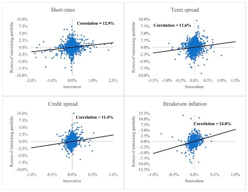
We provide additional plots to show the relation between (market-beta adjusted) returns of mimicking portfolios and innovations in the corresponding macro variables. We rely on our preferred estimation approach, which uses weekly returns and applies Bayesian shrinkage and dynamic weighting (WLS). Figure 2 shows returns of mimicking portfolios on a scatterplot where the horizontal axis corresponds to weekly innovations in macro variables, and the vertical axis corresponds to weekly returns. The plots also indicate correlation coefficients. Across different mimicking portfolios, the correlations of returns with shocks in the corresponding macro variable are above 10%. The inflation mimicking portfolio yields the highest correlation of around 25%. Visual inspection of these scatterplots also suggests that our findings about out of sample macro exposures are not driven by outliers.

Figure 2. Relation between Returns on Macro Mimicking Portfolios and Macro Variables

Designing Equity Portfolios from Stock-Level Measures of Macro Exposures

We have already seen that our macro exposure estimates can reliably distinguish between stocks with high and low exposure to macro risks. This allows us to construct long-only portfolios that come with exposure to the broad stock market index as well as with targeted macro exposures. We test stylised strategies that simply select 30% of the stocks with the highest or lowest macro exposure estimates and weight them equally across all selected stocks. Note that these strategies simply correspond to the long and the short legs of the macro mimicking portfolios introduced above. We refer to such strategies as macro dedicated portfolios. This gives us four portfolios that correspond to high exposure or Macro Exposure(+) to a given variable and four low exposure or Macro Exposure(−) portfolios for the same four state variables.

An alternative to building portfolios from stock-level exposures would be to use a set of existing portfolios and allocate across them based on the estimated macro exposure. Investment practice often uses sector rotation or factor allocation to gain desired macro exposures, as opposed to building dedicated portfolios from stock-level information. We provide a comparison with these alternative approaches to illustrate the importance of creating macro-dedicated portfolios. Note that, when we test allocation across factors or sectors, we use the same robust estimation method for macro exposures that we use to build dedicated portfolios.

The first approach that we compare allocates equal weights across two out of six equity-factor portfolios with the most desirable macro exposures. We consider six factor portfolios: mid-cap, value, high momentum, low volatility, high profitability, and low investment. The single-factor portfolios select 30% of the stocks with the best factor scores and equally weights them. We refer to such strategies as factor allocations. The second approach allocates across sectors following the Thomson Reuters Business classification.¹⁴ We select the three sectors with the most suitable macro exposure from a total of 10 sectors. Sector indices weight stocks by market cap, and we attribute equal weights to each sector. We refer to such strategies as sector allocations.

Table 3 shows the realised macro exposures for these different approaches. Panel A shows results for macro dedicated equity portfolios. The results suggest that dedicated macro portfolios constructed from stock-level data achieve out-of-sample exposures that are in line with the target. For example, the short-rates (+) strategy has a realised beta of 0.20, which is statistically significant with a t-statistic of 2.49. Moreover, all macro dedicated portfolios have statistically significant exposures out of sample, whether targeting positive or negative exposure.

Table 3. Realised Macro Exposures of Different Equity Macro Strategies

United States 19 June 1970–30 June 2022	Short Rates	Term Spread	Credit Spread	Breakeven Inflation
Panel A: macro dedicated portfolios
Macro Exposure +	0.20*	1.07**	1.31**	4.56**
	(2.49)	(6.39)	(4.44)	(4.68)
Macro Exposure −	−0.60**	−0.26*	−0.97**	−0.81**
	(−6.49)	(−2.08)	(−3.13)	(−2.64)
Differences in Macro Exposures	0.81**	1.33**	2.28**	5.37**
	(5.25)	(4.96)	(3.94)	(4.22)
Panel B: factor allocation
Macro Exposure +	0.01	0.48**	0.35	1.71**
	(0.12)	(3.71)	(0.99)	(4.15)
Macro Exposure −	−0.28**	0.07	−0.48	0.20
	(−3.12)	(0.54)	(−1.67)	(0.93)
Differences in Macro Exposures	0.29*	0.41*	0.84	1.51**
	(2.32)	(2.27)	(1.82)	(3.23)
Panel C: sector allocation
Macro Exposure +	0.43**	0.84**	0.51	6.41**
	(3.69)	(3.63)	(0.97)	(5.33)
Macro Exposure −	−0.51**	−0.36	−0.88	0.55
	(−3.71)	(−1.45)	(−1.49)	(0.87)
Differences in Macro Exposures	0.94**	1.19**	1.39	5.86**
	(5.21)	(3.55)	(1.75)	(4.31)

Notes: The analysis has been done from 19 June 1970 to 30 June 2022. The only exception is breakeven inflation, for which the analysis starts in 31 March 2002. The out-of-sample macro exposures are estimated in a bivariate regression that includes the market factor and innovations in corresponding macro variable. Standard errors are adjusted for heteroskedasticity and autocorrelation following Newey and West (1987). We follow Andrews (1991) when determining data-dependent bandwidth/lag truncation parameters, which are estimated in a first-order autoregressive model (AR(1)) with a maximum likelihood method. The null hypothesis that the differences in macro exposures are zero is tested by Welch’s test. The Welch’s t-statistics may not equal to the t-statistics of the null hypothesis that the macro mimicking portfolio has zero exposure, reported in Table 2. Statistical significance is indicated by a single asterisk (*) for results that are significant on a 5% basis and by double asterisks (**) for results that are significant on a 1% basis.

If we look at panel B of Table 3, we see quite different results. Even though factor allocation strategies mostly display exposures that have the desired sign, they are often statistically insignificant. For example, the allocation strategy is unsuccessful at capturing positive exposures to short rates and credit spread. In addition, factor allocations were unable to achieve negative exposures to breakeven inflation and the term spread.

Sector allocations produce relatively better performance than factor allocation, as shown in panel C of Table 3. The exposures are in line with the objective for three out of four variables, but sometimes they are not statistically significant. Some exposures are the opposite of what was targeted: The sector allocation targeting negative exposure to breakeven inflation comes with positive out-of-sample exposure.

Our results clearly indicate that selecting stocks based on their macro exposures leads to more consistent and pronounced exposures out of sample than allocating across sectors or factors. This may not be surprising, as sectors or factors were not designed to proxy certain macroeconomic risks, whilst this is the case for macro dedicated portfolios. Macro exposures of sectors or factors are not heterogenous enough to create portfolios with reliable macro sensitivity out of sample. Industry practices that try to achieve these macro exposures through sector rotation or factor allocation strategies might be problematic. We find that the cross-section of stocks provides more diverse exposures that allow creating portfolios with stronger out-of-sample macro exposures, consistently across all macro variables.

As an alternative to selecting a fixed number of stocks according to estimated exposures, one may also consider the statistical significance of exposure estimates when selecting stocks. We also test mimicking portfolios where the long and short legs are formed by selecting only those stocks that have statistically significant exposure estimates at the 5% level.¹⁵

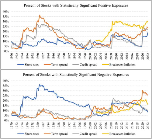
Before forming portfolios, we first consider whether we have enough stocks in our universe at each point in time with either positive or negative exposures to the given macro variable. Having a sufficient number of stocks is necessary to ensure that our test portfolios are not overly concentrated. Figure 3 below reports the percentage of stocks in our universe that have statistically significant exposures. We observe that, at times, stocks with significantly negative or positive exposure to a given macro variable only make up less than 5% of the universe. This means that the mimicking portfolio would be highly concentrated. To avoid extreme levels of concentration, we impose that at least 5% of the stocks are selected.

Figure 3. Percentage of Stocks with Statistically Significant Macro Exposures across Time

Table 4 repeats the analysis from and reports out-of-sample exposures of macro dedicated portfolios. We report the out-of-sample exposures of portfolios that select a fixed number of stocks (30%) in panel A, whilst panel B focusses on portfolios that only select stocks with statistically significant macro exposures (but at least 5% of stocks).

Table 4. Reliability of Macro Beta Estimates Using an Alternative Method to Form Mimicking Portfolios

United States 19 June 1970–30 June 2022	Short-Rates	Term Spread	Credit Spread	Breakeven Inflation	Average
Panel A: macro dedicated portfolios—30% EW selection
Macro exposure +	0.20*	1.07**	1.31**	4.56**	1.78
	(2.49)	(6.39)	(4.44)	(4.68)	(4.50)
Macro exposure −	−0.60**	−0.26*	−0.97**	−0.81**	−0.66
	(−6.49)	(−2.08)	(−3.13)	(−2.64)	(−3.59)
Panel B: macro dedicated portfolios—EW significant exposures (min 5%)
Macro exposure +	0.38**	1.22**	1.73**	5.65**	2.25
	(2.60)	(4.78)	(3.12)	(5.23)	(3.93)
Macro exposure −	−0.72**	−0.60*	−0.81	−0.86	−0.75
	(−5.31)	(−2.37)	(−1.61)	(−0.77)	(−2.51)

Notes: The analysis has been done from 19 June 1970 to 30 June 2022. The only exception is breakeven inflation, for which the analysis starts in 31 March 2002. The out-of-sample macro exposures are estimated in a bivariate regression that includes the market factor and innovations in corresponding macro variable. The estimation frequency and frequency when calculating realised exposures are the same. Standard errors are adjusted for heteroskedasticity and autocorrelation following Newey and West (1987). We follow Andrews (1991) when determining data-dependent bandwidth/lag truncation parameters, which are estimated in a first-order autoregressive model (AR(1)) with a maximum likelihood method. Statistical significance is indicated by a single asterisk (*) for results that are significant on a 5% basis and double asterisks (**) for results that are significant on a 1% basis.

EW = equal weighted.

As expected, we find that more aggressive stock selection improves the magnitude of out-of-sample betas on average. However, there is no improvement when looking at average t-statistics of realised exposures. Using a fixed threshold of selecting 30% of stocks allows for better diversified portfolios, which leads to more out-of-sample robustness than forming concentrated portfolios of stocks that have the most significant exposures on a stand-alone basis.

Why Do Equity-Style Factors Not Suffice to Manage Macro Risks?

The factor allocation strategies in Table 3 do not allow managing macro risks as efficiently as macro dedicated strategies. However, it has been documented that different factors do react differently to economic conditions (see Amenc et al. 2019). Below, we show why—despite this heterogeneity—factor allocation is not a sufficient tool to manage macro exposures. We consider six long-only factors constructed in a highly liquid universe, namely the mid-cap, value, momentum, low volatility, high profitability, and low investment factor portfolios. In addition to the long-term realised macro exposures, we report ex-ante estimated exposures at each quarter. Table 5 reports realised long-term exposures as well as descriptive statistics for ex-ante exposures estimated each quarter. For reference, we also report the exposure of macro dedicated portfolios for each macro variable.

Table 5. Ex-Ante and Realised Exposures of Equity-Style Factors

19 June 1970–30 June 2022	Mid-Cap	Value	Momentum	Low Volatility	High Profitability	Low Investment	Average across 6 Factors	Macro Exposure (+)	Macro Exposure (−)
Exposures to short rates
Realised exposure	−0.16*	−0.28**	−0.06	−0.32**	0.07	−0.24**	−0.17	0.20*	−0.60**
Mean ex-ante exposure	−0.12	−0.17	−0.12	−0.22	0.09	−0.18	−0.12	1.45	−1.75
Min	−0.75	−0.64	−0.60	−0.76	−0.31	−0.68	−0.50	0.35	−3.84
25th percentile	−0.37	−0.39	−0.35	−0.40	−0.07	−0.40	−0.30	0.61	−2.41
Median	−0.13	−0.19	−0.18	−0.26	0.04	−0.22	−0.15	0.98	−1.45
75th percentile	0.00	−0.03	0.01	−0.02	0.28	−0.08	0.04	2.26	−1.05
Max	1.11	1.35	1.12	0.44	0.71	1.34	0.39	4.84	−0.81
Exposures to term spread
Realised exposure	0.42**	0.67**	0.06	0.26*	0.12	0.44**	0.33*	1.07**	−0.26*
Mean ex-ante exposure	0.21	0.28	0.18	0.10	0.17	0.22	0.25	2.04	−1.59
Min	−0.80	−0.85	−0.73	−0.75	−0.77	−0.77	−0.74	0.97	−4.75
25th percentile	−0.07	0.05	−0.13	−0.24	0.03	−0.02	0.05	1.26	−2.43
Median	0.19	0.27	0.17	0.08	0.14	0.15	0.23	2.05	−1.12
75th percentile	0.52	0.52	0.47	0.46	0.31	0.50	0.50	2.42	−0.67
Max	0.96	0.98	1.04	0.93	0.95	0.92	0.88	4.80	−0.27
Exposures to credit spread
Realised exposure	−0.22	0.04	0.14	0.58*	−0.61**	0.29	0.04	1.32**	−0.97**
Mean ex-ante exposure	0.11	0.30	0.22	0.46	−0.16	0.32	0.35	3.86	−3.43
Min	−1.77	−1.85	−1.78	−1.18	−1.93	−1.41	−1.55	2.21	−7.12
25th percentile	−0.64	−0.41	−0.41	−0.17	−0.53	−0.24	−0.22	2.92	−4.96
Median	0.29	0.51	0.29	0.54	−0.09	0.52	0.49	3.76	−3.40
75th percentile	0.65	0.80	0.77	0.96	0.24	0.81	0.74	4.73	−1.77
Max	2.30	2.24	2.28	2.47	1.27	2.00	1.87	6.52	−1.21
Exposures to breakeven inflation (31 March 2002–30 June 2022)
Realised exposure	0.23**	0.20*	0.36*	0.34	0.20**	0.42**	0.29**	4.54**	−0.82**
Mean ex-ante exposure	1.30	1.39	0.86	0.27	1.01	1.00	0.65	5.37	−2.58
Min	0.39	0.17	−0.51	−0.49	0.11	0.07	0.24	3.50	−4.19
25th percentile	0.76	0.62	0.30	−0.08	0.79	0.45	0.36	4.56	−2.93
Median	1.40	1.57	0.75	0.33	1.00	1.13	0.45	5.23	−2.53
75th percentile	1.75	1.91	1.40	0.63	1.31	1.28	0.91	5.82	−2.04
Max	2.29	3.02	2.46	1.04	1.83	2.59	1.63	8.67	−1.78

Notes: The equity-style factor portfolios select 30% of the stocks with the best factor scores and equally weights them. The equity universe consists of 500 largest stocks in the U.S. and is reviewed quarterly, on the third Friday of March, June, September, and December. The percentile values are taken from the time series of ex-ante beta estimates for a given equity factor and a given macro variable. Realised exposures were computed over the full sample. Realised macro exposures are estimated in a bivariate regression using weekly observations, where explanatory variables are the market excess return and innovations in a given macro variable. Ex-ante exposure measures are estimated following our proposed methodology. Statistical significance is indicated by a single asterisk (*) for results that are significant on a 5% basis and double asterisks (**) for results that are significant on a 1% basis. We test statistical significance only for full-sample realised exposures. Values set in bold are realised (i.e., ex-post) exposures. Realised exposures of dedicated macro portfolios are highlighted in yellow when they are unique in the sense that none of the equity style factors provide significant exposures with the same sign.

As expected, realised macro exposures are different across equity factors, as shown in Table 5. For example, the low-volatility portfolio comes with a credit spread beta of 0.58, whilst the high-profitability portfolio has beta of −0.61 to innovations in term spread. However, once we look at the average exposures across six equity factor portfolios, the realised exposures become small and statistically insignificant in most cases.

Second, dedicated macro portfolios are always able to achieve stronger realised exposures than any of the six equity factors, whether positive or negative. This suggests that if investors’ objective is to gain pronounced exposure to a given macro variable, they would be better off using macro dedicated strategies. In addition, selecting amongst equity factors does not allow gaining both positive and negative exposures to three out of four macro variables. For example, we find that four out of six factor portfolios come with significantly positive exposure to the term spread, but none of the factors provide significantly negative exposure. This is true not just for the term spread but also for short-rates and breakeven inflation. Hence, using standard equity factors not only delivers relatively weak macro exposures, but it also renders some exposure targets infeasible.

Last, but not least, we find that the macro exposures of equity-style factors are not necessarily consistent across time. We find that the estimated ex-ante macro exposures of most equity factors take both positive and negative values in different periods of our sample. For instance, the 25th percentile of ex-ante betas to the credit spread are negative for all six factors, whilst the 75th percentiles are positive for all factors. This implies that, for 25% of the quarters in our sample, a factor has a positive credit spread beta, but for 25% of the quarters the same factor has a negative beta. We observe similar instability across time in ex-ante exposure to other macro variables, at least for some of the equity factors.

Because their macro exposures are relatively weak and unstable over time, standard equity factors may not be suitable tools to build portfolios that target macro exposures. In contrast, dedicated macro portfolios allow for more effective targeting of macro exposures.

Conditional Performance of Dedicated Macro Exposure Portfolios

We now show how desired macro exposures translate into returns of the macro dedicated portfolios. We split the sample into positive and negative surprises (top/bottom 25%) for each given macro variable. A portfolio that targets positive exposure to a given macro variable should outperform the market when the surprise in this variable is positive, and vice versa. Figure 4 reports average annualised returns adjusted for market exposure for all dedicated macro portfolios in respective conditions of macro surprises. For example, the term spread (+) portfolio outperforms its market benchmark by around 12 percentage points per year when surprises in term spread are positive. Similarly, we see the opposite for term spread (−) portfolio, which underperforms the market in positive surprises but outperforms when it is meant to (i.e., when the surprises in term spread are negative). We see that all portfolios outperform in macro conditions that they target. The only exception is the short-rates (+) portfolio that comes with statistically insignificant, albeit positive, outperformance during the times of positive interest rate surprises. The inflation (+) portfolio demonstrated a very strong performance when expected inflation rises: The annualised returns are more than 20 percentage points higher than that of the market portfolio during positive inflation shocks.

Figure 4. Conditional Relative Performance of Macro Dedicated Portfolios

The plot shows average annualised returns of macro dedicated portfolios after adjusting for their market exposure (CAPM beta). The analysis was done from 19 June 1970 to 30 June 2022 for all portfolios, except for the inflation portfolios, for which the analysis starts on 31 March 2002. Positive (negative) surprise periods are defined as calendar weeks (Friday to Friday) when the change in a given macro variable was amongst the top (bottom) 25% of historical observations. Returns that are statistically significant at a 5% level are presented in bars with solid fill, whilst returns that are not statistically significant at 5% are presented in bars filled with diagonal stripes.

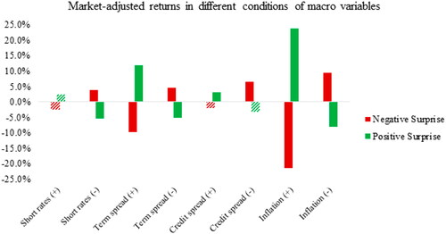
The dedicated macro strategies deliver economically large and statistically significant outperformance when innovations in the targeted variable are in the desired direction, with the exception of short rates (+). Whilst it is beyond the scope of this paper to analyse particular applications of such portfolios, it is clear that the reliable conditionality of macro dedicated portfolios can be of great use for investors. For example, an investor with a large allocation to credit could offset the losses by investing their equity portfolio in a credit spread (+) strategy, thus outperforming the market during the periods of positive surprises in credit spread. As another example, for an active investor who thinks that inflation expectations will rise unexpectedly in the future, using an inflation (+) portfolio can provide strong performance for their equity portfolio in times when surprises in breakeven inflation are positive.

Overall, the results suggest that macro dedicated portfolios can provide strong and economically significant outperformance over the market portfolio in desired macro conditions. Investors who are concerned with substantial movements in certain macroeconomic variables can benefit by investing in the corresponding macro dedicated portfolio.

Performance and Risk of Dedicated Macro Exposure Portfolios

The macro dedicated portfolios deliver positive outperformance over the market portfolio during times of surprises, either positive or negative, in a targeted macro variable. We now analyse the unconditional performance and risk of these strategies. As a reference, we use the cap-weighted market portfolio.

Table 6 reports unconditional performance of various macro dedicated portfolios. The results suggest that the performance of macro-dedicated portfolios is not markedly different from the reference index. The statistical significance test of the differences in Sharpe ratios indicates that only the credit spread (+) portfolio has a Sharpe ratio greater than the market portfolio. Risk-adjusted performance of all other macro dedicated portfolios is statistically indistinguishable from that of the reference index. The deviations in relative returns are small, ranging between 0.53% and 1.76%. The p values of relative returns are all above 5%, meaning that none of these return differences are statistically significant.

Table 6. Unconditional Performance of Macro Dedicated Portfolios

United States 19 June 1970–30 June 2022	Cap-Weighted	Short Rates (+)	Short Rates (−)	Term Spread (+)	Term Spread (−)	Credit Spread (+)	Credit Spread (−)
Absolute return	10.70%	11.35%	11.87%	11.28%	11.93%	12.45%	11.22%
Volatility	17.08%	18.61%	16.69%	18.78%	16.51%	15.97%	18.97%
Sharpe ratio	0.35	0.36	0.43	0.35	0.44	0.48*	0.34
p value of the differences in Sharpe ratio	–	83.6%	22.6%	76.0%	10.8%	1.5%	60.2%
Relative return	–	0.66%	1.18%	0.59%	1.23%	1.76%	0.53%
p value of relative return	–	25.9%	29.7%	40.9%	19.4%	9.3%	32.5%
Tracking error	–	5.45%	6.73%	7.16%	5.52%	5.85%	5.90%
Information ratio	–	0.12	0.17	0.08	0.22	0.30	0.09

Notes: The table reports performance and risk measures for macro dedicated portfolios. The analysis was done using daily returns in USD, from 19 June 1970 to 30 June 2022. The annualised returns are computed as geometric average, whilst the statistical tests of differences in Sharpe ratio and relative returns use arithmetic average. The p values of the differences in Sharpe ratios are computed following the methodology proposed by Ledoit and Wolf (2008). Statistical significance of the differences in relative returns and Sharpe ratios is indicated by a single asterisk (*) for results that are significant on a 5% basis and double asterisks (**) for results that are significant on a 1% basis.

Note that we have omitted the inflation portfolios from this analysis because they are only available staring in March 2002. Table 7 reports the same analysis for inflation portfolios, but over the period starting on 31 March 2002 and ending on 30 June 2022. Our findings are very similar to those above. The differences in Sharpe ratio as well as relative returns are statistically insignificant. Overall, we do not find that any macro dedicated strategies bear significant cost relative to the market index in our sample period.

Table 7. Unconditional Performance of Inflation Targeting Portfolios

United States 31 March 2002 to 30 June 2022	Cap-Weighted	Inflation (+)	Inflation (−)
Absolute return	7.88%	6.31%	9.42%
Volatility	19.65%	26.12%	18.61%
Sharpe ratio	0.33	0.19	0.44
p value of the differences in Sharpe ratio	–	16.3%	17.3%
Relative return	–	−1.56%	1.55%
p value of relative return	–	89.1%	34.6%
Tracking error	–	10.37%	5.56%
Information ratio	–	−0.15	0.28

Notes: The table reports performance and risk measures for macro dedicated portfolios. The analysis was done using daily returns in USD, from 31 March 2002 to 30 June 2022. The annualised returns are computed as geometric average, whilst the statistical tests of differences in Sharpe Ratio and relative returns use arithmetic average. The p-values of the differences in Sharpe ratios are computed following the methodology proposed by Ledoit and Wolf (2008). Statistical significance of the differences in relative returns and Sharpe ratios is indicated by a single asterisk (*) for results that are significant on a 5% basis, and double asterisks (**) for results that are significant on a 1% basis.

Table 8 shows the results of seven-factor regressions that include the market as well as six long-short equity factors widely used in the literature. We find that market betas of dedicated macro portfolios range between 0.87 and 1.06. Exposures to other equity factors are small in magnitude for most strategies and rarely exceed 0.30 in magnitude. Another pattern that we observe consistently across all strategies is a positive exposure to the size factor, which is expected because we weight the selected stocks equally.

Table 8. Factor Exposure Analysis of Macro Dedicated Portfolios

United States 19 June 1970^a–30 June 2022	Short Rates (+)	Short Rates (−)	Term Spread (+)	Term Spread (−)	Credit Spread (+)	Credit Spread (−)	Inflation (+)	Inflation (−)
Unexplained	1.14%	1.53%	1.45%	1.36%	2.00%*	1.13%	1.54%	0.37%
Market	1.05**	0.87**	0.94**	0.99**	0.88**	1.04**	1.06**	0.99**
Size	0.15**	0.37**	0.32**	0.15**	0.24**	0.19**	0.27**	0.17**
Value	0.08	0.06	0.26**	−0.05	0.19**	0.07	0.37**	−0.10**
Momentum	0.05**	−0.10**	0.07**	−0.10**	−0.05*	0.06**	0.14**	−0.12**
Volatility	−0.01	−0.05**	−0.28**	0.30**	0.00	−0.11**	−0.16**	0.22**
Profitability	−0.32**	0.15**	−0.12**	−0.14**	0.20**	−0.30**	−0.44**	0.12**
Investment	−0.08*	−0.01	0.15**	−0.24**	0.04	−0.20**	−0.10*	−0.10**
R-squared	90.95%	85.87%	89.79%	88.22%	87.24%	90.96%	92.26%	93.26%

Notes: The table reports factor exposures of macro dedicated portfolios. The analysis was done using weekly returns in USD, from 19 June 1970 to 30 June 2022. ^aThe only exception is portfolios targeting exposure to breakeven inflation, for which the analysis starts in 31 March 2002. Factor intensity is the sum of all factor exposures except for the market factor. The unexplained returns are annualised. Statistical significance is indicated by a single asterisk (*) for results that are significant on a 5% basis and double asterisks (**) for results that are significant on a 1% basis.

Table 8 also provides interesting insights regarding the multifactor alphas of macro dedicated portfolios. In particular, we find that seven out of eight portfolios have an alpha that is statistically indistinguishable from zero. The credit spread (+) portfolio has a positive and significant alpha in the multifactor model. None of the eight portfolios display a significantly negative multifactor alpha over the sample period. This suggests that investors, who had focussed on targeting their desired macro exposure, would not have born a cost of underperformance (negative alpha), regardless of which of the eight possible exposures they had targeted.

Our results imply that equity investors can target desired macro exposures without paying a premium. To further evaluate the potential performance implications of targeting macro exposures, we also estimate the trading costs of macro dedicated portfolios. Table 9 reports transaction costs as well as performance measures net of transaction costs for different macro strategies. We follow Corwin and Schultz (2012) and Chung and Zhang (2014) to estimate the proxy of effective bid-ask spread.¹⁶ These two approaches have been shown to yield to reliable and accurate proxies of intra-day effective spreads. The measures proposed by Chung and Zhang (2014) is more accurate, but it can only be applied starting in 1993, because the closing bid and ask prices that are used for computing the effective bid-ask spread are only available from that point. Hence, we rely on effective spreads following Corwin and Schultz (2012) before 1993 and following Chung and Zhang (2014) afterwards.

Table 9. Performance of Macro Dedicated Portfolios Net of Transaction Costs

31 December 1977–30 June 2022	Broad U.S. Cap-Weighted	Short Rates		Term Spread		Credit Spread
		(+)	(−)	(+)	(−)	(+)	(−)
Gross annual return	11.41%	12.09%	11.84%	11.63%	12.53%	13.13%	11.60%
Net annual return	11.39%	11.79%	11.60%	11.31%	12.21%	12.85%	11.26%
Annual transaction cost	1 bps	30 bps	24 bps	32 bps	32 bps	27 bps	34 bps
Annual turnover	2.90%	51.77%	42.67%	53.49%	52.79%	48.45%	56.22%
Net Sharpe ratio	0.40	0.40	0.43	0.37	0.49	0.53*	0.37
p value	–	80.6%	63.2%	43.7%	13.3%	2.6%	38.1%
Net multifactor alpha	0.00%	0.80%	0.81%	0.64%	1.18%	1.84%*	0.43%
p value	–	36.3%	39.3%	48.0%	19.1%	3.5%	62.1%

Notes: Transaction cost is estimated as a difference in gross annualised performance and annualised performance net of transaction costs. The stock-level transaction costs are estimated from daily prices. Prior to 1993, we use the methodology proposed by Corwin and Schultz (2012), whilst after 1993, we rely on the methodology of Chung and Zhang (2014). The reported turnover is a one-way turnover, computed quarterly and annualised by multiplied the average by 4. The p values of the differences in Sharpe ratios are computed following the methodology proposed by Ledoit and Wolf (2008). The analysis was done from 31 December 1977 to 30 June 2022. The analysis starts only in 1977 due to data quality and availability of intra-day high and low prices. Statistical significance of the differences in net Sharpe ratios and net multifactor alphas is indicated by a single asterisk (*) for results that are significant on a 5% basis and double asterisks (**) for results that are significant on a 1% basis.

The results in Table 9 indicate that the annual transaction costs of macro dedicated portfolios are below 35 basis points. Therefore, the impact on the performance is mild, and our conclusions from the analysis of gross returns remain intact. In particular, macro strategies do not come with significantly lower Sharpe ratios, and the multifactor alphas are statistically indistinguishable from zero for the portfolios targeting either positive or negative exposures to the short rates and term spread. The only significant performance difference observed in our analysis is for the credit spread (+) portfolio, which outperforms the market and the multifactor benchmark, even after accounting for transaction costs.

The results are similar in Table 10, where we focus on inflation portfolios over a more recent period. We find no evidence that portfolios that come with positive or negative exposure to breakeven inflation cause reduction in the performance relative to the market portfolio or a multifactor benchmark. Note that the transaction costs for inflation portfolios are substantially smaller than those reported in Table 9. This is mainly due to the differences in sample period.¹⁷ The transaction costs have declined dramatically over recent decades, as the market structure has improved, in particular through the reduction in minimum tick size for trading (see Bruno et al. 2019). Therefore, historical estimates of trading costs, such as the ones in Table 9, are inflated compared to the costs that investors face today. Also note that we did not apply further implementation rules, such as buffers in stock selection or investability rules that reduce the amount of trading at rebalancing. Such rules could be used to further reduce transaction costs in practice (see Novy-Marx and Velikov 2016).

Table 10. Performance of Inflation Portfolios Net of Transaction Costs

31 March 2002–31 December 2019	Broad U.S. Cap-Weighted	Breakeven Inflation
		(+)	(−)
Gross annual return	8.20%	7.71%	9.12%
Net annual return	8.20%	7.56%	8.99%
Annual Transaction cost	<1 bps	14 bps	13 bps
Annual turnover	3.50%	47.58%	43.29%
Net Sharpe ratio	0.36	0.25	0.42
p value	–	33.8%	32.6%
Net multifactor alpha	0.00%	1.41%	0.25%
p value	–	35.6%	80.2%

Notes: Transaction cost is estimated as a difference in gross annualised performance and annualised performance net of transaction costs. The stock-level transaction costs are estimated from daily prices following the methodology proposed by Chung and Zhang (2014). Statistical significance of the differences in net Sharpe ratios and net multifactor alphas is indicated by a single asterisk (*) for results that are significant on a 5% basis and double asterisks (**) for results that are significant on a 1% basis.

Overall, our findings are consistent with empirical evidence in a recent study by Herskovic, Moreira, and Muir ([2019) which finds that hedging exposures to different macro risks, including the credit spread and term spread, has little to no impact on expected returns. Moreover, the empirical asset pricing literature has established a set of workhorse models to explain the cross -section of stock returns that have evolved over time (from the Fama and French [1993] three-factor model to the Fama and French [2018] six-factor model or the Hou, Mo, Xue, and Zhang [2021] five-factor model). Whilst these models draw on slightly different sets of equity-style factors, none of them includes macroeconomic factors, such as the variables studied in this paper. This is in line with the idea that such macroeconomic factors do not offer risk compensation over and above what the typical equity-style factors capture.

In contrast, several papers argue that some macroeconomic factors may be separately priced in the cross-section. Boons (2016) finds that the term spread and credit spread are priced factors in a broad cross-section of U.S. equities (including small- and micro-cap stocks), but the short rate is not. Petkova (2006) finds that exposures to short rates are priced along with term spread, but the credit spread is not. Such studies, however, have not led to a generally accepted inclusion of macro factors in workhorse models used to explain the cross-section of stock returns. In our setting, where we analyse a universe of liquid stocks and account for a broad set of style factors, macro exposures are not associated with separate risk premiums. An interesting avenue for future research is to assess risk premia for macro exposures whilst accounting for the fact that risk premia may be dynamic and may change sign over time (see, e.g., Boons et al. 2020, 2021).

Conclusion

We have proposed a methodology to estimate stock-level exposures to different macroeconomic risks. We rely on innovations in forward-looking variables that quickly incorporate investors’ expectations about economic conditions, such as short-term interest rates, the term spread, the credit spread, and breakeven inflation. To capture exposure of stocks to these macro surprises, we apply statistical tools to improve robustness. We then construct dedicated portfolios from the resulting firm-level measures of macro exposure. Such equity strategies come with statistically and economically significant exposures out of sample.

Our robust measurement procedure delivers a more robust and reliable classification of stocks than standard estimation approaches. When constructing equity portfolios that target high or low macroeconomic exposure, our procedure leads to more than 40% higher realised out-of-sample exposures and more than 70% improvements in t-statistics associated with these exposures, compared to naïve estimation.¹⁸

Our approach of building dedicated portfolios using stock-level exposures also captures macro exposures more reliably than using off-the-shelf building blocks, such as sector or factor indices. We show that allocating across sectors or factors leads to weaker exposures than our dedicated macro portfolios and sometimes even leads to exposures that are inconsistent with the objective. The reason behind this is that sectors or factors are not designed to discriminate assets by macroeconomic risk exposures, whilst the stock-level approach can fully exploit the heterogeneity of exposures in the cross-section of equities.

In addition, our proposed strategies are fully systematic and do not rely on common beliefs or the discretionary choices of an asset manager.

Finally, we showed that our macro exposure strategies do not suffer from lower performance compared to a broad equity portfolio. The stand-alone returns of eight macro exposure strategies as well as their Sharpe ratios are not significantly different from the market portfolio in our sample. They also do not come with negative alphas in a multifactor model that includes the usual style factors. Our conclusions hold when accounting for trading costs of dedicated macro portfolios.

Overall, we show that our macro exposure measures can add value for investors with a dual objective, which is to harvest the long-term equity premium and protect their total portfolio from sudden changes in economic conditions (or bet in favour of certain economic conditions). In practice, such measures could be used for a variety of applications such as tilting long-only portfolios to target the desired macro sensitivities.

Acknowledgements

We would like to thank Noël Amenc, two anonymous referees, and the editors of the journal for helpful comments and suggestions.

Disclosure statement

No potential conflict of interest was reported by the author(s).

Additional information

Notes on contributors

Mikheil Esakia

Mikheil Esakia is quantitative research analyst at Scientific Beta, Nice, France.

Felix Goltz

Felix Goltz is research director at Scientific Beta and associate researcher at EDHEC Business School, Nice, France.

Notes

1 An incomplete list includes Novy-Marx (2013) and Bali, Brown, and Caglayan (2014).

2 As we will see later, the statistical adjustments proposed by Boons (2016) are similar to the ones we use. However, there are two key differences between our analyses. First, we use higher frequency for estimation than Boons (2016). It has been shown that higher frequency increases sample size and improves the accuracy (see Levi and Welch 2017). Second, Boons (2016) looks at all common stocks in the CRSP universe, which is much larger than our investable universe that consists of the largest 500 stocks in U.S. Our mission is more difficult because distinguishing amongst high- and low-exposure stocks in a smaller universe requires more precision.

3 For clarity, we focus on a single objective of targeting macro exposures. An interesting area for future research would be to assess how investors can combine objectives in terms of factor exposures aimed at improving unconditional returns with objectives in terms of macro exposures aimed at targeting conditional returns.

4 We have also analysed the out-of-sample reliability of exposures to various other macro variables using our estimation approach, and the results are reported in the Online Supplemental Material. First, we have estimated exposures of stocks to macro variables that are based on market prices that reflect investor expectations, such as commodities, interest rates on U.S. Treasuries with different maturities and inflation swaps. Our estimation approach leads to highly reliable out-of-sample exposures to these variables. In addition, we have looked at aggregate economic indicators based on macro fundamentals, such as the Aruoba-Diebold-Scotti Business Conditions Index (ADS) and Bloomberg Weekly Consumer Comfort Index (CCI). These two macro variables aim to nowcast the economic activity, such as growth (for ADS) and consumer confidence (CCI), and are available at daily and weekly frequency, respectively. Exposures we measure with respect to these variables are not necessarily reliable out of sample. This suggests that relying on market-based macro variables that reflect shocks in investor expectations is important to successfully detect a link with equity returns (see Amenc et al. [2019] for a detailed discussion of this argument).

5 Amenc et al. (2019) have not included expected inflation in their analysis.

6 For a more detailed discussion on each state variable, please refer to Amenc et al. (2019).

7 Various studies document that term spread predicts returns on long-term asset classes. See, for example, Fama and French (1989) for equities and bonds, Campbell (1996) for human capital, Hong and Yogo (2012) for commodities, and Ang, Nabar, and Wald (2013) for real estate.

8 We have also tested innovations from VAR(1,1) model, and our findings are unaffected by this change. Using VAR model was proposed by Campbell (1996) in this context and has been followed by various other studies more recently (e.g., Petkova 2006, Boons 2016). Each macro variable is modelled as a linear function of the past values of all macro variables considered.

9 We also require that at least 208 weekly observations are available for a given stock, which is equivalent to 80% of total observations in 5 years. For other estimation approaches, which use OLS or monthly frequency, we also require that at least 80% of the total observations in a five-year period are available.

10 Beyond information in returns, one might also exploit information in company risk disclosures using textual analysis. We have conducted additional analysis augmenting our returns-based measures using textual analysis. This approach also delivers robust exposures out of sample but is not reported here for brevity.

11 Our universe excludes ADRs.

12 We also tested the out-of-sample reliability of our estimation approach in an Asian universe. Results can be found in the Online Supplemental Material.

13 Results of this long-term analysis can be found in the Online Supplemental Material.

14 The sectors are (1) energy, (2) basic materials, (3) industrials, (4) cyclical consumer, (5) non-cyclical consumer, (6) financials, (7) healthcare, (8) technology, (9) telecoms, and (10) utilities.

15 Note that we use exposure estimates before shrinkage, because the standard errors of those exposures correspond to “unshrunk” beta estimates. Such an approach can be considered an alternative to shrinkage, as both approaches try to account for the uncertainty around point estimate.

16 Our analysis accounts for the effective bid-ask spread, but ignores the costs such as brokerage commissions, exchange taxes, and financial transaction taxes. Such costs are difficult to account for because they may vary widely depending on the bargaining power of investors.

17 We report more detailed analysis of turnover and transaction costs over different time periods for all macro dedicated portfolios in the Online Supplemental Material.

18 The average out-of-sample beta increases from 1.71 to 2.45, whilst the average t-statistic increases from 2.53 to 4.39, as shown in Table 2.

References

- Amenc, N., M. Esakia, F. Goltz, and B. Luyten. 2019. “Macroeconomic Risks in Equity Factor Investing.” The Journal of Portfolio Management 45 (6): 39–60. doi:10.3905/jpm.2019.1.092.
- Andrews, D. W. K. 1991. “Heteroskedasticity and Autocorrelation Consistent Covariance Matrix Estimation.” Econometrica: Journal of the Econometric Society 59 (3): 817–858. doi:10.2307/2938229.
- Ang, A., M. Brière, and O. Signori. 2012. “Inflation and Individual Equities.” Financial Analysts Journal 68 (4): 36–55. doi:10.2469/faj.v68.n4.3.
- Ang, A., N. Nabar, and S. Wald. 2013. “Searching for Common Factor in Public Private Real Estate Returns.” The Journal of Portfolio Management 39 (6): 120–133. doi:10.3905/jpm.2013.39.6.120.
- Bali, T. G., S. J. Brown, and M. O. Caglayan. 2014. “Macroeconomic Risk and Hedge Fund Returns.” Journal of Financial Economics 114 (1): 1–19. doi:10.1016/j.jfineco.2014.06.008.
- Boons, M. 2016. “State Variables, Macroeconomic Activity, and the Cross Section of Individual Stocks.” Journal of Financial Economics 119 (3): 489–511. doi:10.1016/j.jfineco.2015.05.010.
- Boons, Martijn, Fernando Duarte, Frans De Roon, and Marta Szymanowska. 2020. “Time-Varying Inflation Risk and Stock Returns.” Journal of Financial Economics 136 (2): 444–470. doi:10.1016/j.jfineco.2019.09.012.
- Bruno, G., M. Esakia, and F. Goltz. 2019. Towards Cost Transparency: Estimating Transaction Costs for Smart Beta Strategies. Nice, France: Scientific Beta.
- Campbell, J. Y. 1987. “Stock Returns and the Term Structure.” Journal of Financial Economics (18) (2): 373–399. doi:10.1016/0304-405X(87)90045-6.
- Campbell, J. Y. 1996. “Understanding Risk and Return.” Journal of Political Economy 104 (2): 298–345. doi:10.1086/262026.
- Chen, N.-F., R. Roll, and S. A. Ross. 1986. “Economic Forces and the Stock Market.” The Journal of Business 59 (3): 383–403. doi:10.1086/296344.
- Chousakos, Kyriakos, and Daniel Giamouridis. 2020. “Harvesting Macroeconomic Risk Premia.” The Journal of Portfolio Management 46 (6): 93–109. doi:10.3905/jpm.2020.1.149.
- Chung, Kee H., and Hao Zhang. 2014. “A Simple Approximation of Intraday Spreads Using Daily Data.” Journal of Financial Markets 17 : 94–120. doi:10.1016/j.finmar.2013.02.004.
- Corwin, Shane A., and Paul Schultz. 2012. “A Simple Way to Estimate Bid‐Ask Spreads from Daily High and Low Prices.” The Journal of Finance 67 (2): 719–760. doi:10.1111/j.1540-6261.2012.01729.x.
- Devarajan, M., V. Naik, A. Nowobilski, S. Page, and N. Pedersen. 2016. Factor Investing and Asset Allocation – a Business Cycle Perspective. Charlottesville, VA: The CFA Institute Research Foundation. http://library.asue.am/open/5334.pdf.
- Estrella, A., and M. R. Trubin. 2006. “The Yield Curve as a Leading Indicator: Some Practical Issues.” Current Issues in Economics and Finance, Federal Reserve Bank of New York 12 (5). https://msuweb.montclair.edu/∼lebelp/EstrellaYieldCurveIndicatorFRBNY200608.pdf.
- Fama, E. F. 1981. “Stock Returns, Real Activity, Inflation, and Money.” The American Economic Review 71 (4): 545–565.
- Fama, E. F., and K. R. French. 1989. “Business Conditions and Expected Returns on Stocks and Bonds.” Journal of Financial Economics 25 (1): 23–49. doi:10.1016/0304-405X(89)90095-0.
- Fama, E. F., and K. R. French. 1993. “Common Risk Factors in the Returns on Stocks and Bonds.” Journal of Financial Economics 33 (1): 3–56. doi:10.1016/0304-405X(93)90023-5.
- Fama, E. F., and K. R. French. 1997. “Industry Costs of Equity.” Journal of Financial Economics 43 (2): 153–193. doi:10.1016/S0304-405X(96)00896-3.
- Fama, E. F., and K. R. French. 2018. “Choosing Factors.” Journal of Financial Economics 128 (2): 234–252. doi:10.1016/j.jfineco.2018.02.012.
- Herskovic, B., A. Moreira, and T. Muir. 2019. Hedging Risk Factors (Working paper). https://doi.org/10.2139/ssrn.3148693
- Hong, H., and M. Yogo. 2012. “What Does Futures Market Interest Tell Us About the Macroeconomy and Asset Prices?” Journal of Financial Economics 105 (3): 473–490. doi:10.1016/j.jfineco.2012.04.005.
- Hou, K., H. Mo, C. Xue, and L. Zhang. 2021. “An Augmented q-Factor Model With Expected Growth.” Review of Finance 25 (1): 1–41. doi:10.1093/rof/rfaa004.
- Jurczenko, Emmanuel, and Jérôme Teiletche. 2020. Macro Factor-Mimicking Portfolios (Working paper). https://doi.org/10.2139/ssrn.3363598
- Keim, D. B., and R. F. Stambaugh. 1986. “Predicting Returns in the Stock and Bond Markets.” Journal of Financial Economics 17 (2): 357–390. doi:10.1016/0304-405X(86)90070-X.
- Ledoit, O., and M. Wolf. 2008. “ Robust Performance Hypothesis Testing With the Sharpe Ratio.” Journal of Empirical Finance 15 (5): 850–859. doi:10.1016/j.jempfin.2008.03.002.
- Levi, Y., and I. Welch. 2017. “Best Practice for Cost-of-Capital Estimates.” Journal of Financial and Quantitative Analysis 52 (2): 427–463. doi:10.1017/S0022109017000114.
- Longstaff, F. A. 2004. “The Flight-to-Liquidity Premium in U.S. Treasury Bond Prices.” The Journal of Business 77 (3): 511–526. doi:10.1086/386528.
- Newey, W. K., and K. D. West. 1987. “A Simple, Positive Semi-Definite, Heteroskedasticity and Autocorrelation Consistent Covariance Matrix.” Econometrica 55 (3): 703–708. doi:10.2307/1913610.
- Novy-Marx, R. 2013. “The Other Side of Value: The Gross Profitability Premium.” Journal of Financial Economics 108 (1): 1–28. doi:10.1016/j.jfineco.2013.01.003.
- Novy-Marx, R., and M. Velikov. 2016. “A Taxonomy of Anomalies and Their Trading Costs.” Review of Financial Studies 29 (1): 104–147. doi:10.1093/rfs/hhv063.
- Petkova, R. 2006. “Do the Fama–French Factors Proxy for Innovations in Predictive Variables?” The Journal of Finance 61 (2): 581–612. doi:10.1111/j.1540-6261.2006.00849.x.
- Swade, Alexander, Harald Lohre, Mark Shackleton, Sandra Nolte, Scott Hixon, and Jay Raol. 2021. “Macro Factor Investing With Style.” The Journal of Portfolio Management 48 (2): 80–104. doi:10.3905/jpm.2021.1.306.
- Ung, D., and P. Luk. 2016. “What is in Your Smart Beta Portfolio? A Fundamental and Macroeconomic Analysis.” The Journal of Index Investing 7 (1): 49–77. doi:10.3905/jii.2016.7.1.049.
- Vasicek, O. A. 1973. “A Note on Using Cross-Sectional Information in Bayesian Estimation of Security Betas.” The Journal of Finance 28 (5): 1233–1239. doi:10.1111/j.1540-6261.1973.tb01452.x.