Factor Replication with Industry Stratification

Abstract

Factor investing exploits asset pricing anomalies to enhance fund returns. Unlike traditional market capitalization indexes, factors have onerous replication costs. We consider the impact of omitting costly, small stocks by industry in stratified factor-replicating portfolios. Such industry stratification achieves broader industry coverage and lowers tracking error compared with competing approaches. We show that the improvement in tracking error is due to enhanced industry coverage, not risk exposure, resulting in substantial economic benefits.

Keywords:

• Benchmark fidelity
• cost reduction
• dynamic replication
• factor indexation
• factor replication
• industry stratification
• portfolio costs
• tracking error

PL Credits: 2.0:

Introduction

Worth billions of dollars, factor investing is used by fund managers to exploit asset pricing anomalies and enhance fund returns (Cerniglia and Fabozzi 2018; Arnott et al. 2019). However, factor replication is challenging to implement efficiently. We introduce a new methodology (industry stratification [IS]) to replicate factors accurately while reducing replication costs.

This methodology is important for factors because, in contrast to traditional indexation, they suffer onerous replication costs that severely erode their performance (Novy-Marx and Velikov 2019). Chen and Velikov (2022) demonstrate that factor returns of nearly 70 basis points per month before costs are diminished to only 6 basis points per month after costs. To harvest any remaining factor returns, investors must reproduce factors at a low cost. Portfolio stratification is one way to reduce replication costs. Stratification removes the most costly stock from a factor portfolio. Naïve stratification (NS) incrementally removes the costliest stock in the entire factor replication portfolio. In contrast, IS removes the costliest stock by industry.

Stratification also has other benefits apart from reducing costs. For example, it is important for many applications when trading a smaller portfolio is beneficial, such as exchange-traded fund unit creation, dynamic hedging, and various others when trading quickly is required.

Theoretically, a portfolio’s returns are commensurate with its industry exposure, which proxies for risk class (Modigliani and Miller 1958; Ross 1988; Lewellen, Nagel, and Shanken 2010). By design, IS preserves industry exposure, and high-fidelity factor replication ensues (Ahn, Conrad, and Dittmar 2009). Investment managers already employ industry coverage to enhance traditional index replication (Michaud 1989; Larsen and Resnick 1998; Chan, Lakonishok, and Swaminathan 2007). Anticipating factors, Rudd (1980) decomposes benchmark tracking error (TE) into two components and provides a theory that suggests NS mitigates the first, while IS reduces the second component of TE.

We compare IS with two competing stratification techniques for factor replication: NS and optimized stratification using linear programming (LP; see van Montfort, Visser, and van Draat 2008; Rossbach and Karlow 2019; Stentoft and Wang 2019). IS, NS, and LP have differing goals. The primary purpose of NS is to reduce the costs of factor replication by strictly removing the smallest, costliest stocks in the entire replicating portfolio. In contrast, the primary goal of IS is to both retain similar industry exposures to the factor benchmark and eliminate each industry’s smallest, costliest stocks. LP’s explicit goal is to minimize TE and replication costs by optimizing the portfolio weights of a stratified portfolio, irrespective of industry (Michaud 1989). Alternative ways of reducing transaction costs (banding [Novy-Marx and Velikov 2016] or staggered implementation similar to one used in Jegadeesh and Titman [1993]) also exist.

Our analysis comparing these three stratification techniques demonstrates the superiority of IS. Not only does IS achieve greater industry coverage, but it also results in the lowest after-cost TE. This enhanced TE is due to broader benchmark industry coverage, as opposed to differences in risk exposure. We show that the TE reduction for IS dominates NS’s cost-reduction benefits. Finally, we demonstrate the substantial economic benefits of IS.

This work should be of great interest to practitioners. Factors are a popular institutional fund investment vehicle worth billions of dollars. Since factor replication, unlike traditional indexation, is especially expensive to implement (Novy-Marx and Velikov 2019), reducing replication costs is crucial for viable factors. The significant IS enhancements we report are comparable to the after-cost factor returns available (Chen and Velikov 2022). Relatively large economic value accrues to factor replication using IS. We conclude that IS provides both enhanced TE and substantial economic value.

Data and Methodology

Quasi-Russell 1000 Index Benchmark and Factor Portfolios

The benchmark portfolios in this study are based on the most popular Russell U.S. equity index. This index was created in 1984 by the Frank Russell Company to represent the broad U.S. equity market. By 2018, $8.1 trillion had been invested using Russell indexes as the benchmark. The Russell 1000 index comprises the top 1,000 stocks by market capitalization, using the annual (June) reconstitution criterion provided by Russell Investments (which primarily relies on market capitalization). We implement the Quasi-Russell 1000 (QR1000). This index selects the largest 1,000 stocks by market capitalization but assumes monthly rather than annual index reconstitution.¹ We use Center for Research in Security Prices/Compustat data where necessary. We analyze a period of more than 30 years, from June 1990 to December 2021. We use the Global Industry Classification Standard (GICS) for IS (Bhojraj, Lee, and Oler 2003; Hrazdil, Trottier, and Zhang 2013). We also obtain robust results for the largest 3,000 stocks (QR3000).

We focus on the Russell 1000 benchmark for a variety of reasons. First, it is among the most popular and widely followed market indexes in the United States. Second, many funds and exchange-traded funds (ETFs) implement factor indexing (e.g., equal-weighted indexing) using the Russell 1000 as a benchmark, such as the Guggenheim Russell 1000 Equal Weight (EW) ETF, which uses the Russell 1000 EW Index as its underlying benchmark.

We study and compare IS using numerous factor portfolios that represent those commonly available via ETFs (see Online Supplemental Material Appendix A). These include the following long-only factor indexes: (1) the composite fundamental (FI; see Arnott et al. 2005), (2) the EW (DeMiguel et al. 2009), (3) the diversity weighted (DW; see Fernholz et al. 1998), (4) the diversified risk parity weighted (DRPW; see Maillard, Roncalli, and Teïletche 2010), (5) diversified minimized variance (DMV; see Clarke, de Silva, and Thorley 2013), (6) quality (QLTY; see Sloan 1996), and (7) momentum (MOM; see Jegadeesh and Titman 1993; Fama and French 1993).

Similar to Ang et al. (2021), when using the QR1000, we use long-only factor indexes and report $1 billion portfolio results, with monthly rebalancing. Regardless of the factor, the benchmark is always costless (i.e., does not consider implicit or explicit costs), monthly rebalanced, and 100% inclusive of all stocks.

Portfolio Stratification Methodologies

To validate IS, we compare it to NS and LP. NS should significantly enhance after-cost factor returns, since it strictly removes the smallest, costliest stocks. However, it removes more stocks in certain industries and hence does not accurately reproduce benchmark industry coverage. Such industries become underrepresented in naïve factor-replicating portfolios, creating unbalanced industry exposures in the factor replication portfolio. This leads to unrepresentative industry basis assets, low-fidelity factor benchmark returns, and ultimately, relatively poor benchmark tracking.

To ascertain which approach tracks the benchmark best, we must measure TE. A rich literature has explored how to measure benchmark TE. Academics have often focused on minimizing σ²(TE) or σ(TE) (Roll 1992). Theoretically, compared to such metrics, linear deviation TE metrics enjoy various benefits. We adopt Sharpe’s (1971) mean absolute deviation metric for pragmatism, ease of interpretation, and robustness and focus on linear deviation rather than TE variance. We use the following linear TE model (Sharpe 1971; Rudolf, Wolter, and Zimmermann 1999): (1) $${TE}_i=\mathrm{ }\mathit{MAD}\left({TE}_i\right)=\mathrm{ }\frac{1}{T}{\sum }_{t=1\mathrm{ }}^T\mathit{Abs}\mathrm{ }|R_{i,t}\mathrm{ }–\mathrm{ }{R}_{B,t}|$$(1) where the $R_{i,t}$ values are the returns of the ith stratified replicator and the $R_{B,t}$ values are the returns of the appropriate 100% zero-cost benchmark.

We compare the TEs of IS, NS, and LP replicating portfolios at various stratification levels. Since the smallest and most expensive stocks are incrementally removed to construct different industry-stratified portfolios, we compare their TEs after costs with the relevant, ideal, costless benchmark. The benefit of doing this iteratively across increasing stratification levels is that we can observe both the marginal effect of including increasingly smaller, costlier stocks on the stratified portfolios’ costs and measure the ensuing industry coverage, observing the consequent differences in TE.

The creation of industry-stratified factor-replicating portfolios involves three steps: (1) ranking each stock by cost in each industry (which facilitates the rank cost of trading each stock relative to its industry peers), (2) using the industry stock rank from step 1 to determine which stocks will be included in the factor-replicating portfolio for each stratification level, and (3) using the stocks from step 2 to calculate the TE difference compared to the costless benchmark for each stratification level by employing a portfolio simulation.

IS relies on stable, contemporaneous industry classification to generate stable, robust, and accurate investment weights for the IS factor-replicating portfolio.² Given that we use GICS for our industry categorization, our IS methodology (see step 1 above) requires that we order each stock in each industry by cost. Our fundamental tenet is that mimicking industry exposure is crucial for high-fidelity factor replication. Given that factor replication is expensive, we wish to remove the costliest stock from the replicating portfolio while retaining the highest possible industry and return fidelity to the factor benchmark. However, in what order should we remove stocks from each industry to reduce costs? There are many ways to measure the cost of trading stocks. Trading costs comprise explicit and implicit costs (see below). Ideally, we want a cost metric that encompasses both. We consider three cost metrics: market capitalization, volatility, and spread. Each cost metric we consider measures different aspects of trading costs. Given that a stock’s market capitalization is inversely proportional to its trading costs (Amihud and Mendelson 1989), we verify that this cost metric provides the lowest absolute TE of all those considered, and we therefore focus on it.

To accurately compare factor replication approaches, we must consider transaction costs in our analysis. The transaction cost reduction of factor replication portfolios can be achieved using a combination of trading less (i.e., reducing turnover) and/or trading cheaper (i.e., reducing the cost of turnover). Novy-Marx and Velikov (2019) evaluate three methods that exploit both channels, highlighting the “extreme importance” of including transaction costs for an accurate factor investment analysis. Factor studies that neglect the inherent costs of dynamic factor portfolio replication do so at their peril, because “when paper portfolio moves to live trading transaction costs start to play a very important role [italics added]” (Arnott et al. 2019, 19).

We include costs and rectify this common but important omission. We include both explicit and implicit costs in our evaluations of factor replication portfolios. We model the total transaction costs as the sum of those due to explicit costs³ and those due to implicit costs (i.e., price impacts): (2) $$T{C}_{i,t}=\mathrm{ }C\left(\mathit{Trade}\mathrm{ }\mathit{Siz}{e}_{i,t}\right)+PI(\mathit{Trade}\mathrm{ }\mathit{Siz}{e}_{i,t,\frac{b}{s}})$$(2) where $T{C}_{i,t}$ is the total transaction cost of trading stock $i$ at rebalancing date $t;$ $C$ represents commissions, which we model as a constant rate paid on the value of all purchases and sales of stock $i$ at time $t;$ and $PI$ is the price impact, which is based on the size decile to which stock $i$ belongs, the trade size $t,$ and the direction of the trade ($\frac{b}{s},$ buy or sell).

Whether Risk Exposure or Industry Coverage Causes TE Improvement

We introduce our methodology to test whether IS leads to more consistent industry coverage of the factor benchmark or whether the improvements are due to risk exposure. We compare the industry coverage of both the NS and IS approaches to the benchmark using the industry concentration index (ICI) to proxy for industry coverage. Kacperczyk, Sialm, and Zheng (2005) were the first to use ICI to proxy for industry portfolio concentration. The ICI measures the aggregate differences in investment across all industries between stratified and benchmark portfolios, as follows: (3) $${\mathit{ICI}}_t=\mathrm{ }{\sum }_{\mathrm{i}=1\mathrm{ }}^{11}{(W_{i,t}\mathrm{ }–\mathrm{ }{\overline{W}}_{i,t})}^2$$(3) where, for industry $i,$ the ICI in month $t$ is the sum of the squared differences between the weights of each of the 11 GICS sectors in the stratified portfolio $(W_{i,t})$ and the weights of the respective sectors in the benchmark portfolio ${(\overline{W}}_{i,t}).$ An ICI value of zero indicates that the concentration of industries in the replication portfolio is the same as that in the benchmark portfolio.

Our fundamental tenet is that replicating industry exposure is crucial for high-fidelity factor replication. Using a regression model (see below), we formally test whether the differences in the TE, (i.e., ΔTE) between the IS and NS (or LP and NS) approaches are due to differences in industry coverage or standard risk exposure.

We estimate the following extended Daniel, Mota, Rottke and Santos (2020) (DMRS) five-factor regression: (4) $$\Delta {TE}_{s,t}^{}\equiv {|TE}_{s,t}^{IS}\left|\mathrm{ }-{|TE}_{s,t}^{NS}\right|={\alpha }_s+b_s{{\mathit{RMRF}}_t^{\mathrm{*}}}_{}+s_s{{\mathit{SMB}}_t^{\mathrm{*}}}_{}+{h_s{{\mathit{HML}}_t^{\mathrm{*}}}_{}}_{}+r_s{{\mathit{RMW}}_t^{\mathrm{*}}}_{}{+{c_s{{\mathit{CMA}}_t^{\mathrm{*}}}_{}}_{}+i}_s\Delta {\mathit{ICI}}_{s,t}^{}+\mathrm{ }{ϵ}_{s,t}$$(4) where

• ΔTE_s,t ≡ ${|TE}_{s,t}^{IS}\left| -{|TE}_{s,t}^{NS}\right|$ is the difference between the absolute TEs from the IS portfolios and those from the NS portfolios for stratification level $s$ in month $t;$

• ${\mathit{RMRF}}_t^{*}$ is the market value-weighted return minus that on the risk-free rate of return (U.S. monthly Treasury bill rate) in month $t,$ using DMRS factor portfolio data;

• ${\mathit{SMB}}_t^{*}$ is the monthly return on small capitalized portfolios minus that of big capitalized portfolios, using DMRS factor portfolio data;

• ${{\mathit{HML}}_t^{*}}_{}$ is the monthly return on portfolios with a high book value to equity minus that on portfolios with a low book value to equity, using DMRS factor portfolio data;

• ${\mathit{RMW}}_t^{*}$ is the monthly return on high-profitability (robust) firms minus that on weak-profitability (weak) firms;

• ${\mathit{CMA}}_t^{*}$ is the monthly return on low-investment (conservative) firms minus that on high-investment (aggressive) firms; and

• ΔICI_s,t ≡ ${\mathit{ICI}}_{s,t}^{IS} -{\mathit{ICI}}_{s,t}^{NS}$ is the difference between the aggregate ICI measure for IS portfolios and that for naïvely stratified portfolios for stratification level $s$ in month $t.$

The dependent variable is the difference in TE between the stratification approaches, ΔTE, for each stratification percentage level. In Equation (4)(4) $$\Delta {TE}_{s,t}^{}\equiv {|TE}_{s,t}^{IS}\left|\mathrm{ }-{|TE}_{s,t}^{NS}\right|={\alpha }_s+b_s{{\mathit{RMRF}}_t^{\mathrm{*}}}_{}+s_s{{\mathit{SMB}}_t^{\mathrm{*}}}_{}+{h_s{{\mathit{HML}}_t^{\mathrm{*}}}_{}}_{}+r_s{{\mathit{RMW}}_t^{\mathrm{*}}}_{}{+{c_s{{\mathit{CMA}}_t^{\mathrm{*}}}_{}}_{}+i}_s\Delta {\mathit{ICI}}_{s,t}^{}+\mathrm{ }{ϵ}_{s,t}$$(4) , the independent variables include the five–risk factor model of DMRS and an additional variable, the ICI variable (see above and Kacperczyk et al. 2005).

These five risk factors are the market beta (RMRF*), the adjusted Fama–French value (HML*), size (SMB*), profitability (RMW*), and investment (CMA*). The additional independent variable is the aggregate difference of the ICI (i.e., coverage), ΔICI.

The key independent variable in Equation (4)(4) $$\Delta {TE}_{s,t}^{}\equiv {|TE}_{s,t}^{IS}\left|\mathrm{ }-{|TE}_{s,t}^{NS}\right|={\alpha }_s+b_s{{\mathit{RMRF}}_t^{\mathrm{*}}}_{}+s_s{{\mathit{SMB}}_t^{\mathrm{*}}}_{}+{h_s{{\mathit{HML}}_t^{\mathrm{*}}}_{}}_{}+r_s{{\mathit{RMW}}_t^{\mathrm{*}}}_{}{+{c_s{{\mathit{CMA}}_t^{\mathrm{*}}}_{}}_{}+i}_s\Delta {\mathit{ICI}}_{s,t}^{}+\mathrm{ }{ϵ}_{s,t}$$(4) is ΔICI, which corresponds to the difference between the industry- and naïvely stratified ICI and represents the aggregate difference of the ICI (i.e., coverage) between the industry- and naïvely stratified approaches. Given that the ICI has a zero lower bound (see Equation (3)(3) $${\mathit{ICI}}_t=\mathrm{ }{\sum }_{\mathrm{i}=1\mathrm{ }}^{11}{(W_{i,t}\mathrm{ }–\mathrm{ }{\overline{W}}_{i,t})}^2$$(3) ) and that we calculate the difference in the ICI (i.e., ΔICI), a negative ΔICI means that the industry-stratified portfolio is closer to benchmark coverage. This is because its ICI value is closer to the zero lower bound than that of the naïvely stratified portfolio.

The asterisk (*) associated with the independent variables in Equation (4)(4) $$\Delta {TE}_{s,t}^{}\equiv {|TE}_{s,t}^{IS}\left|\mathrm{ }-{|TE}_{s,t}^{NS}\right|={\alpha }_s+b_s{{\mathit{RMRF}}_t^{\mathrm{*}}}_{}+s_s{{\mathit{SMB}}_t^{\mathrm{*}}}_{}+{h_s{{\mathit{HML}}_t^{\mathrm{*}}}_{}}_{}+r_s{{\mathit{RMW}}_t^{\mathrm{*}}}_{}{+{c_s{{\mathit{CMA}}_t^{\mathrm{*}}}_{}}_{}+i}_s\Delta {\mathit{ICI}}_{s,t}^{}+\mathrm{ }{ϵ}_{s,t}$$(4) indicates that they are not the standard Fama–French (2015) factors, but DMRS characteristic–adjusted factors. The DMRS approach combines hedge portfolios with characteristic portfolios to form “characteristic-efficient” portfolios. DMRS (2020) claims that these represent better benchmarks for the evaluation of managed portfolios, such as our factor-replicating portfolios, and retain the benefit of the traditional regression-based asset pricing approach without the need for holdings data, which are required when using the characteristics methodology of Daniel and Titman (1997). DMRS characteristic–efficient portfolios use historical covariance and characteristics and thus improve upon their Fama–French counterparts.

Results and Analysis

Comparing Ideal and Costly Factor Benchmarks

In Table 1, four dimensions of the relative performance between each factor’s costless and costly benchmarks (i.e., at 100% stratification) are compared, including performance, turnover, transaction cost, and replication quality metrics.⁴

Table 1. Comparing Costless and Costed Factor Benchmarks for QR1000 IS 100%

	MCWI	FI	EW	DW-1	DW-2	DW-3	DRPW	DMV	MOM	QLTY
Annualized Geometric Ret. (%):	10.89	10.84	10.77	10.92	10.98	10.96	10.81	9.42	8.92	10.74
Annualized Volatility (%):	14.72	15.30	16.84	16.33	15.75	15.16	14.69	13.55	15.74	16.37
Value of $1:	26.14	25.77	25.26	26.41	26.87	26.70	25.60	17.18	14.85	25.07
Ratio to Benchmark:	0.97	0.88	0.81	0.87	0.91	0.95	0.73	0.52	0.41	0.62
Annualized Turnover (%):	12.84	43.01	72.42	54.09	37.24	22.77	93.94	153.31	226.11	120.28
Trade of $1:	26.09	156.37	225.18	167.71	110.35	59.60	322.00	315.81	647.99	412.60
Cost of $1:	0.13	0.91	1.43	0.98	0.59	0.30	2.16	4.40	4.63	3.13
% of Costless:	97.29	87.70	81.36	86.75	91.45	95.14	73.40	52.16	40.87	62.44
Eroded Value:	0.73	3.61	5.79	4.03	2.51	1.36	9.27	15.76	21.48	15.08
Tracking Error Diff Monthly Benchmark (%):	0.01	0.04	0.05	0.04	0.02	0.01	0.08	0.17	0.24	0.12
Information Ratio:	−0.20	−0.92	−1.55	−1.18	−0.74	−0.42	−1.86	−1.82	−4.13	−0.82

Notes: Reducing factor replication costs while maintaining high-fidelity tracking is crucial to attaining viable factors. This table compares four dimensions of the relative performance between each factor’s costless and costly benchmarks (i.e., all stocks or 100% stratification) including performance, turnover, transaction cost, and replication quality metrics. In contrast to Market Capitalized Weighted Indexation, factors do not enjoy automatic rebalancing and require dynamic rebalancing to replicate factors accurately, generating substantial portfolio turnover and corresponding large transaction costs that erode factor performance. After including transaction costs, each benchmark factor suffers severe performance degradation relative to its costless benchmark. The key driver of this performance degradation is turnover. Factor returns are affected in proportion to each factor’s turnover. These results demonstrate, consistent with the extant literature that, after costs, efficient factor replication is crucial for viable factors.

Although the market capitalized weighted index (MCWI) is not a factor, it is included in Table 1 for comparison with the factors. MCWI is an important point of reference to factors, since it represents the theoretically optimal portfolio, has small investment weights to small, costly stocks, and is very cheap to replicate because it benefits from automatic portfolio rebalancing.

In contrast to MCWI, factors do not enjoy automatic rebalancing and require dynamic rebalancing to replicate factors accurately, generating substantial portfolio turnover and corresponding large transaction costs that erode factor performance (Chen and Velikov 2022). Table 1 shows that each factor, after including transaction costs, suffers severe performance degradation relative to its costless benchmark.

The key driver of this performance degradation is turnover. Factor returns are affected in proportion to each strategy’s turnover. The factors with the highest annualized turnover suffer the greatest performance degradation since the combination of large assets under management and turnover leads to a large trading volume and, consequently, severe price impact costs. MCWI belongs to the lowest turnover category. We classify the factors into three additional broad turnover categories: the medium-turnover category includes the FI and the three diversity-weighted factors, the high-turnover category includes the EW and DRPW factors, and the very-high turnover category includes the DMV, MOM, and QLTY factors.

Considering the lowest turnover category, MCWI, first, Table 1 shows that dynamically replicating MCWI after costs provides an extremely high ratio to benchmark value of 0.97. This means that replication trading costs erode very little value of the MCWI replicating portfolios, in contrast to the worst-performing factors, namely, QLTY (0.62), DMV (0.52), and MOM (0.41). The reason for MCWI’s relatively high ratio to benchmark is also clear from Table 1, since the annualized turnover for MCWI is between 5% and 15% of the three highest turnover factors reported. Next, the percentage of costless value describes the proportion of a portfolio that remains after costs. For MCWI, 97% of the value remains, in contrast to the three worst-performing factors, which retain only approximately 40% to 60% of their value after costs. While MCWI suffers some degradation in the quality of benchmark tracking due to the trading costs associated with portfolio turnover, as measured by the information ratio (−0.20), its degradation is far more benign than that of the most severely affected factor, MOM (−4.13).

Three main conclusions are gleaned from an analysis of Table 1. First, it is much more difficult to replicate factors than MCWI after costs. Second, as smaller stocks become more prominent in a portfolio, factor replication becomes more onerous due to the consequent increased costs of turnover. Finally, those factors with high turnover (see above) suffer the worst performance degradation relative to their costless benchmark. These results serve to empirically motivate our IS approach. Given this performance degradation due to turnover and ensuing costs, consistent with the literature (Chen and Velikov 2022), the goal of reducing factor replication costs while maintaining high-fidelity tracking is crucial to attaining viable factors.

Comparing the Coverage of Each Industry When Incrementally Removing Stocks Using NS and IS

Pronounced heterogeneity in stock market capitalization exists among industries. A few large stocks characterize certain industries, while other industries contain many small stocks. We demonstrate below that, due to this heterogeneity, despite removing the strictly smallest, costliest stocks for the factor benchmark, NS induces considerable industry bias, ultimately leading to incomplete industry basis asset coverage (Ahn, Conrad, and Dittmar 2009), low-fidelity factor replication, and increased factor replication TE.

Using the procedure described in Section Portfolio Stratification Methodologies, Table 2 presents the market capitalization by stratification for each industry. The stratification percentage (top row) in Table 2 represents the percentage (100%—percentage) of the largest (smallest) stocks retained (removed) in the factor portfolio. Table 2 reports the coverage for NS (Panel A) and IS (Panel B). Each GICS industry is represented by a different row, while each column represents the cumulative stratification level (i.e., the percentage of the largest stocks retained in the replication portfolio). Before weighting each stock according to the various factor indexation weighting schemes (see Online Supplemental Material Appendix A and F), we remove (retain) the smallest (largest) stock by using its percentile market–capitalized stratification rank. For a given percentile stratification rank, NS (Panel A) removes the smallest percentile-ranked stock in the entire factor replication portfolio, irrespective of industry. In contrast, IS (Panel B) removes the smallest stock by percentile rank in each industry. For a given stratification level, the number of stocks removed is held constant in both approaches.

Table 2. Percentage Coverage by Industry for QR1000 Using NS (Panel A) and IS (Panel B) by GICS

GICS/% Strat.	10	20	30	40	50	60	70	80	90	100
A: QR1000 percentage coverage using NS, by GICS
Energy	33%	52%	52%	52%	67%	67%	67%	67%	67%	100%
Materials	80%	100%	100%	100%	100%	100%	100%	100%	100%	100%
Industrials	49%	69%	79%	79%	79%	79%	79%	79%	100%	100%
Consumer Discretionary	57%	81%	100%	100%	100%	100%	100%	100%	100%	100%
Consumer Staples	35%	44%	44%	60%	84%	84%	100%	100%	100%	100%
Health	28%	42%	63%	63%	73%	100%	100%	100%	100%	100%
Financials	47%	61%	66%	79%	100%	100%	100%	100%	100%	100%
Information Technology	27%	30%	34%	41%	62%	62%	62%	78%	78%	100%
Communication Services	30%	46%	67%	82%	100%	100%	100%	100%	100%	100%
Utilities	100%	100%	100%	100%	100%	100%	100%	100%	100%	100%
Real Estate	100%	100%	100%	100%	100%	100%	100%	100%	100%	100%
B: QR1000 percentage coverage using IS, by GICS
Energy	59%	75%	85%	92%	95%	97%	99%	99%	100%	100%
Materials	44%	59%	70%	78%	85%	90%	94%	97%	99%	100%
Industrials	60%	76%	84%	90%	93%	96%	97%	99%	99%	100%
Consumer Discretionary	57%	73%	82%	88%	92%	95%	97%	98%	99%	100%
Consumer Staples	62%	77%	85%	90%	94%	97%	98%	99%	100%	100%
Health	53%	74%	85%	91%	94%	96%	98%	99%	100%	100%
Financials	61%	76%	85%	90%	93%	96%	98%	99%	100%	100%
Information Technology	70%	84%	90%	94%	96%	98%	99%	99%	100%	100%
Communication Services	54%	76%	85%	92%	95%	97%	98%	99%	100%	100%
Utilities	42%	62%	73%	80%	86%	91%	94%	97%	99%	100%
Real Estate	0%	71%	71%	86%	86%	94%	94%	97%	97%	100%

Notes: Using Global Industry Classification Standard (GICS) industry classification, we see the cumulative market capitalization for each percentile stratification level for naïve (NS) and industry stratification (IS). In bold is the stratification level where a threshold coverage of greater than 75% of industry market capitalization is attained. IS results in higher industry coverage at lower stratification. In contrast, NS induces a strong industry selection bias toward industries with large stocks, resulting in unbalanced industry exposure. Since IS provides better factor benchmark industry coverage than NS, it should provide higher fidelity returns to benchmark factors.

To designate a complete or threshold industry coverage, we require a notional 75% market capitalization coverage for an industry. The industry coverage of NS is presented in Panel A of Table 2 and highlights that threshold industry coverage is not uniform among industries. Some industries have high coverage, whereas others have low coverage; that is, different GICS industries achieve threshold industry coverage at markedly different stratification percentiles (see Table 2 figures in bold).

Next, we consider threshold coverage when using IS. Panel B of Table 2 shows that, for most industries, threshold coverage is achieved at much lower stratification percentiles when using IS than when using NS (the results are even more pronounced for the QR3000). This finding is not surprising, since it results directly from the IS methodology that ensures that each industry is highly covered.

These results are very important since they suggest that the NS procedure, which retains the largest stock in a factor replication portfolio, irrespective of industry, will induce a strong industry selection bias toward industries with large stocks. Ultimately, we shall see (see Section “Comparing is with NS”) that this results in unbalanced industry exposure and, consequently, unrepresentative basis asset risk exposure, creating poor levels of TE for factor-replicating portfolios. These results bode well for IS. Since IS provides better industry coverage than NS, these preliminary results suggest that IS should provide greater fidelity to benchmark factors than NS does.

Comparing IS with NS

It is unclear whether, relative to NS, the better industry coverage obtained with IS outweighs any increased costs. By construction, IS includes larger, costlier stock than NS, which removes the strictly smallest from the entire factor. This means that the cost savings associated with NS might outweigh the TE improvements of IS. We demonstrate (below) that, after costs, IS always enjoys lower TE compared with NS.

Since it is among the best known (and costliest) of all the factors to replicate (see Table 1), we focus exclusively on EW in Figure 1 (see Table 3 for other factors). It shows that industry-stratified EW always has a lower TE than the naïvely stratified replication portfolio (converging at 100%), with the optimized LP TE being the worst of the three stratification approaches.

Figure 1. TE for EW Factor Using IS, NS, and LP with QR1000

Notes: Due to onerous replication costs, investors must accurately reproduce factors efficiently. To reduce replication costs, portfolio stratification includes only a portion of the entire factor portfolio. Here, we compare factor replication quality for industry stratification (IS), naïve stratification (NS), and linear programming optimization (LP) using tracking error (TE) by stratification level. NS incrementally removes the smallest, costliest stock in the entire factor replication portfolio. IS removes the most costly stock by industry. LP optimizes stock weights in the stratified replication portfolio by minimizing the tracking error (TE). IS, NS, and LP have differing goals. The primary purpose of NS is to reduce the costs of factor replication by strictly removing the smallest, costliest stocks in the entire replicating portfolio. The primary goal of IS is to both retain similar industry exposures to the factor benchmark and eliminate each industry’s smallest, costliest stocks. LP’s explicit goal is to minimize the TE. For the equal weight factor (EW), IS provides the lowest TE for each stratification level, demonstrating the importance of industry coverage for accurate stratified factor replication.

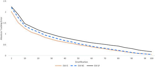
Table 3. Monthly Index Tracking Error (TE, ΔTE) between IS and NS Portfolios for the QR1000 Market Capitalized Ranking

	FI		EW		DW-1		DW-2		DW-3
%	IS	NS	IS	NS	IS	NS	IS	NS	IS	NS
Stratification	ΔTE		ΔTE		ΔTE		ΔTE		ΔTE
10%	0.69	0.77	1.29	1.4	1.17	1.26	1	1.08	0.81	0.87
	−8**		−11**		−10**		−8**		−5**
40%	0.27	0.28	0.64	0.72	0.55	0.61	0.45	0.49	0.33	0.36
	−1*		−8**		−6**		−4**		−3**
70%	0.11	0.12	0.33	0.35	0.27	0.29	0.21	0.22	0.14	0.15
	−1*		−3**		−2**		−1**		−1**

Table

	DRPW		DMV		MOM		QLTY
%	IS	NS	IS	NS	IS	NS	IS	NS
Stratification	ΔTE		ΔTE		ΔTE		ΔTE
10%	1.11	1.22	1.08	1.19	1.27	1.41	1.23	1.35
	−12**		−10*		−13**		−12**
40%	0.56	0.62	0.62	0.66	0.63	0.69	0.63	0.68
	−6**		−4**		−6**		−5**
70%	0.29	0.31	0.4	0.41	0.35	0.38	0.33	0.35
	−2**		−1		−3**		−2**

Notes: These results validate the core intuition of our industry stratification (IS) methodology and demonstrate the general applicability and benefits of IS over naïve stratification (NS) for factor replication. This table presents the tracking error (TE) and TE difference (ΔTE) for 10%, 40%, and 70% stratification levels, and includes two-sided p values using a Wilcoxon matched pairs test (with *indicating significance at the 5% level and **significance at the 1% level). For almost all factors and stratifications, IS leads to a highly statistically significant lower TE than NS. The TE difference between IS and NS, ΔTE, is nearly always negative and significant indicating that IS has a lower TE than NS.

In Table 3, we show that IS attains a lower TE than NS for all the factors. Table 3 reports the industry-stratified and naïvely stratified TE (see Equation (1)(1) $${TE}_i=\mathrm{ }\mathit{MAD}\left({TE}_i\right)=\mathrm{ }\frac{1}{T}{\sum }_{t=1\mathrm{ }}^T\mathit{Abs}\mathrm{ }|R_{i,t}\mathrm{ }–\mathrm{ }{R}_{B,t}|$$(1) ) for each factor index by stratification, and, below it, the difference in the TE values between IS and NS (i.e., ΔTE) is provided in basis points, with the corresponding statistical results of whether H₀: ΔTE = 0 is true (generated using the two-sided Wilcoxon matched pairs test and recorded in Table 3 with * for 5% significance and ** for 1% significance).

For all factors and stratifications, IS leads to a highly statistically significant lower TE than NS. The TE difference between IS and NS, ΔTE, is always negative and significant (apart from DMV at 70% stratification), indicating (given the zero lower bound on TE) that IS has a lower TE than NS. Such consistent results validate the core intuition of our IS methodology and demonstrate the general applicability and advantages of IS over NS for factor replication. How these ΔTE values translate to economic benefits is considered in Section “Economic Enhancement of Industry-Stratified Portfolios”.

For 10% stratification, Table 3 reports that most factors provide IS ΔTE enhancements of about 1.5% per annum. The IS enhancement to ΔTE diminishes at larger stratification levels (i.e., greater than 70%), since the replicating portfolios converge. However, for very low stratification levels (e.g., 5% stratification), ΔTE represents enhancements to factor portfolio returns of almost 3% per annum. Lower stratifications are the most important as they are most likely to be used by fund managers. Additional improvement in TE occurs for the portfolio of greater breadth (i.e., the QR3000).⁵ These results are robust. We also show that the results hold when alternative cost measures (i.e., volatility and spread) are used.

The key results in Table 3 are presented in Figure 2. In Figure 2, we note that the difference between the TEs, ΔTE, of the industry and naïvely stratified portfolios is almost always negative. Since the TE has a zero lower bound by construction, the prevalent negative difference between these TEs means that NS has a larger absolute TE than IS for all stratification levels. Consistent with theory, we observe better TEs for almost all factor indexes provided in Table 3 and Figure 2. This result is crucial since it demonstrates the utility and consistency of our novel factor IS methodology.

Figure 2. ΔTE for All Factors with QR1000

Notes: Reducing factor replication costs by simply removing the most costly, small stocks leads to inaccurate factor replication. Instead, it is important to remove the most costly, small stock by industry, not simply the overall smallest stock. The differences in absolute tracking error, $\Delta \mathrm{TE},$ for the industry (IS) and naïve (NS) stratified portfolios, $\Delta \mathrm{TE}=\left|{\mathrm{TE}}_{\mathrm{IS}}\right|\text{-}\mathrm{ }\left|{\mathrm{TE}}_{\mathrm{NS}}\right|,$ by stratification level is shown. The value of $\Delta \mathrm{TE}$ is almost always less than zero for all factors, denoting enhanced TE for IS versus NS. The prevalent negative difference between $\Delta \mathrm{TE}$ means that NS has a larger TE than IS for all factors for almost all stratification levels.

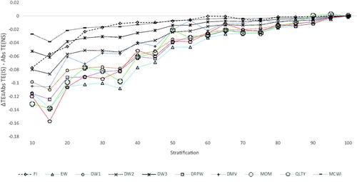
When we compare the various factors in Figure 2, the greatest relative benefit (i.e., most negative ΔTE) of IS arises for EW, and the least for MCWI because of its very low turnover (see Table 1), with the other factors enjoying a range of benefits between them. It is unclear why different benefits of IS accrue to different factors in varying amounts. We will show in the next section that NS’s poor industry coverage, which is due to heterogeneous industry market capitalization, is accentuated for certain factor strategies, such as EW, MOM, and QLTY, which result in them having the most negative ΔTE values (see Figure 2).

Attributing ΔTE to ΔICI

We know from the previous section that IS provides a lower absolute TE than NS. If our IS narrative is accurate, industry coverage, and not standard risk exposure, should be primarily responsible for the lower TE. This is because, by construction, IS provides better industry coverage of the benchmark than NS (see Table 2), spanning the factor benchmark’s industry basis assets more completely (Ahn, Conrad, and Dittmar 2009) and resulting in higher-fidelity returns to the benchmark.

However, stratification can lead to inadvertent tilts to the standard risk factors that drive replication returns. Such inadvertent risk tilts could be responsible for the enhanced returns and, ultimately, IS’s superior TE (observed in Table 3), and not better industry coverage. Therefore, next we ascertain whether risk exposure or industry coverage is responsible for the enhanced tracking of IS observed.

To begin, we focus on industry coverage. We compare the industry coverage of both NS and IS to factor benchmarks. We use the ICI to proxy for industry coverage, where the ICI measures the aggregate differences between stratified and benchmark portfolios in investment across all industries (see Equation (3)(3) $${\mathit{ICI}}_t=\mathrm{ }{\sum }_{\mathrm{i}=1\mathrm{ }}^{11}{(W_{i,t}\mathrm{ }–\mathrm{ }{\overline{W}}_{i,t})}^2$$(3) ). The closer the ICI is to zero, the closer the stratified portfolio is to the factor benchmark industry coverage. To better understand the industry coverage between the two stratification approaches, we narrow our focus on ΔICI, the difference in the ICI between the industry-stratified and naïvely stratified portfolios for each factor.

Figure 3 shows the ΔICI value at each stratification level for each factor portfolio. The difference between IS and NS in the ICI (i.e., ΔICI) is always negative for all factor portfolios.⁶ This result is noteworthy because it means that IS always provides higher-fidelity industry coverage to the benchmark factor portfolio than NS for all factors and at every stratification level. This result agrees with both intuition and theory and confirms that superior industry coverage is directly due to our IS methodology. Although it is impossible to consider an exhaustive set of factors, we are confident that, due to the compelling intuition of IS, this result can be generalized to all factors, not just those considered here.

Figure 3. ΔICI for All Factors with QR1000

Notes: Naïve stratification (NS) retains the largest stock in a factor replication portfolio, irrespective of industry, inducing a strong industry selection bias toward industries with large stocks. This industry selection bias is responsible for the poor performance of the NS methodology. Here, we see the differences in industry coverage (ΔICI; see Kacperczyk et al. (2005)) for the industry stratification (IS) and NS portfolios, ${\Delta \mathrm{ICI}\equiv \mathrm{ }\mathrm{ICI}}^{\mathrm{IS}}-{\mathrm{ICI}}^{\mathrm{NS}}\mathrm{ }$ by stratification for each factor are always negative. This demonstrates that IS provides closer industry coverage to the factor benchmark than NS.

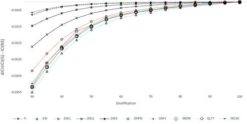
Importantly, as shown in Figure 3, the most negative ΔICI values occur for EW and then DRPW, MOM, and QLTY—which all have similar values—and finally, DMV, and DW − 1. This means that these factor portfolios derive the greatest enhanced industry coverage from IS (vis-à-vis NS), since the relatively large negative ΔICI values imply that they are much closer to benchmark industry coverage than their naïvely stratified counterparts. Interestingly, both MCWI and the FI have ΔICI values closest to zero for each stratification percentile, suggesting they derive the least benefit from IS. These results are broadly consistent with the TE results in Table 3 and Figure 2. They support our narrative that high-fidelity industry coverage with the benchmark is primarily responsible for the superior TE of IS.

Next, we consider the regression results (Equation (4)(4) $$\Delta {TE}_{s,t}^{}\equiv {|TE}_{s,t}^{IS}\left|\mathrm{ }-{|TE}_{s,t}^{NS}\right|={\alpha }_s+b_s{{\mathit{RMRF}}_t^{\mathrm{*}}}_{}+s_s{{\mathit{SMB}}_t^{\mathrm{*}}}_{}+{h_s{{\mathit{HML}}_t^{\mathrm{*}}}_{}}_{}+r_s{{\mathit{RMW}}_t^{\mathrm{*}}}_{}{+{c_s{{\mathit{CMA}}_t^{\mathrm{*}}}_{}}_{}+i}_s\Delta {\mathit{ICI}}_{s,t}^{}+\mathrm{ }{ϵ}_{s,t}$$(4) ) that facilitate formal statistical tests of whether industry coverage, standard risk factors, or both are responsible for the difference in the observed TE between the two stratification approaches. As discussed in Section “Whether Risk Exposure or Industry Coverage Causes TE Improvement”, Equation (4)(4) $$\Delta {TE}_{s,t}^{}\equiv {|TE}_{s,t}^{IS}\left|\mathrm{ }-{|TE}_{s,t}^{NS}\right|={\alpha }_s+b_s{{\mathit{RMRF}}_t^{\mathrm{*}}}_{}+s_s{{\mathit{SMB}}_t^{\mathrm{*}}}_{}+{h_s{{\mathit{HML}}_t^{\mathrm{*}}}_{}}_{}+r_s{{\mathit{RMW}}_t^{\mathrm{*}}}_{}{+{c_s{{\mathit{CMA}}_t^{\mathrm{*}}}_{}}_{}+i}_s\Delta {\mathit{ICI}}_{s,t}^{}+\mathrm{ }{ϵ}_{s,t}$$(4) uses state-of-the-art DMRS asset pricing to ascertain whether asset pricing characteristics—and not simply the standard five Fama–French (2015) factor loadings—explain the differences between ΔTE.

Panel A of Table 4 shows the regression results for the EW factor from our starting period, January 1990, to June 2019 (this end date is different from the end date we use throughout the paper because this is when the factor portfolio returns data of DMRS end, according to Kent Daniel’s website at http://www.kentdaniel.net/data.php). For EW, we report only the 10%, 40%, and 70% stratifications (the columns in Table 4).

Table 4. QR1000 EW and LP Factor DMRS Regression

DMRS factor/
% Strat.	10%	40%	70%
A: QR1000 EW Factor DMRS Regression: ΔTE versus αi, βi, hi, si, ri, ci, and ΔICI by stratification %
αi	0.14	−0.03	0.01
βi	−0.01	0.01	0.01
si	0.00	0.01	0.00
hi	0.02	−0.01	−0.01
ri	−0.04	0.00	0.00
ci	−0.02	0.01	0.01
ΔICIi	12.66	18.34	65.80
t(αi)	1.79*	−0.71	0.77
t(βi)	−0.65	2.81**	2.9**
t(si)	−0.09	1.09	−0.41
t(hi)	0.77	−1.20	−1.51
t(ri)	−1.77*	−0.14	0.86
t(ci)	−0.49	0.88	0.90
t(ΔICIi)	3.5**	1.64	3.18**
B: QR1000 LP Factor DMRS Regression: ΔTE versus αi, βi, hi, si, ri, ci, and ΔICI by stratification %
αi	0.05	0.00	0.02
βi	−0.02	−0.02	−0.02
si	−0.01	−0.01	−0.02
hi	0.02	−0.01	−0.01
ri	0.01	−0.05	−0.03
ci	0.08	0.01	0.01
ΔICIi	4.40	146.06	219.57
t(αi)	1.15	−0.09	0.64
t(βi)	−1.26	−1.59	−1.84*
t(si)	−0.26	−0.38	−1.16
t(hi)	0.8	−0.53	−0.69
t(ri)	0.5	−1.98**	−1.7*
t(ci)	1.9*	0.3	0.54
t(ΔICIi)	0.51	16.77**	20.82**

Notes: The importance of industry coverage for high-fidelity factor replication is highlighted. Stratification may lead to inadvertent risk tilts, responsible for the superior tracking error (TE) of IS observed in Table 3. Here, we show that changes in industry coverage, not standard risk factors, explain differences between differences in TE (ΔTE). The dependent variable is ΔTE. The independent variables are the DMRS risk factors and the difference in industry coverage between industry (IS) and naive (NS) stratification, ΔICI. Panel A applies to EW and Panel B to LP. ΔICI is often significant suggesting that differences in industry coverage explain differences in ΔTE (for all factors see Table B.1, Online Supplemental Material Appendix B). LP generates inferior TE due to its poor industry coverage. Its ΔICI coefficient in Panel B is on between 6 and 10 times larger for LP than EW in Panel A.

For the sake of brevity, the DMRS regression results for all the factors are presented in Online Supplemental Material Appendix B. Typical of all the factors across stratification levels, the industry coverage (i.e., ΔICI) coefficients have the greatest number of significant coefficients, with market exposure (i.e., β) also having some contiguous significant coefficients.

We find that for most stratification intervals, and far more frequently than the standard risk factors, the ΔICI differences are significant, consistent (i.e., significant regression coefficients do not oscillate between positive and negative), and broad (i.e., significant regression coefficients are consistent over many stratification intervals) and coincide with statistically significant differences in TE between the two stratification approaches (discussed in Table 3).

Overall, these regression results show the prevalence of positive and significant regression coefficients for ΔICI.⁷ We find strong evidence that changes in industry coverage explain differences between ΔTE, with, on average, about half (and often between one-third and two-thirds depending on the factor) of all stratification levels demonstrating significant industry coverage coefficients across all factors. In contrast, apart from market exposure (i.e., β), the DMRS five risk factors tend not to be significant. To conclude, in this section, we have shown that industry coverage, and not risk exposure, explains the differences in TE (i.e., ΔTE) between IS and NS.

Industry Basis Asset Coverage versus Cost Mitigation

Ideally, a factor replication strategy must both provide low TE to the factor benchmark and reduce factor replication costs. Given the vital role of cost reduction in factor replication (Novy-Marx and Velikov 2019; Chen and Velikov 2022), it is plausible that cost reduction, not TE, is of paramount concern. In this section, we will demonstrate that the IS enhancements to factors documented in previous sections are dominated by replication accuracy, not by reductions in factor replication costs. This is important because it suggests that effective industry coverage of the benchmark factor replication portfolio is the key to the success of the IS methodology, not simply the removal of the smallest and costliest stock in each industry.

Factor replication cost mitigation strategies may reduce turnover, the cost of turnover, or both (Novy-Marx and Velikov 2019). We evaluate whether NS or IS provides better cost mitigation and via which channel. We study cost mitigation using a turnover metric (i.e., annual turnover) and a cost metric (i.e., eroded value) and compare the difference between IS and NS for each metric by percentile stratification. We focus on the relative differences in cost mitigation between IS and NS.

Generally, we find that the erosion in the returns for all the factor replication portfolios is approximately proportional to turnover (see Table 1). The factors with the highest annualized turnover suffer the greatest performance degradation, since the combination of large assets under management and turnover leads to a large trading volume and, consequently, severe price impact costs. As discussed, we can broadly classify the factors in this work into three turnover categories (see Section “Results and Analysis”). However, our focus in this work is not the turnover of the factor replication portfolio per se, but the difference in turnover due to the different stratification methods.

In Table 1, we focus on complementary performance metrics to understand how the different stratification approaches generate different turnover levels and costs of turnover compared with their costless factor benchmark and the conventional, low-turnover MCWI benchmark. The two cost mitigation metrics we use here provide insight into how much trading and at what cost each stratification approach delivers. The first cost mitigation metric is related to turnover: The turnover metric used is the annualized dollar turnover, Annual Turnover, calculated as the average of the total monthly purchases at time t divided by the fund size at t − 1 multiplied by the rebalancing frequency. The second cost mitigation metric is related to the cost of trading: the cost metric we use is the dollar eroded value, Eroded Value, which is the total dollar cost of trading over the entire period of the study. We combine both and report the performance erosion as a consequence.

In Figure 4, for a given stratification level and factor, we focus on the difference between Annual Turnover and Eroded Value for IS and NS.⁸ Panel A of Figure 4 depicts the values of ΔAnnual Turnover and Panel B depicts the values of ΔEroded Value between IS and NS (the results for the QR3000 are similar). These results show that ΔAnnual Turnover and ΔEroded Value are consistently positive across all stratification levels (apart from DMV and MOM at 90% stratification). This means that IS always has a higher annualized turnover and higher eroded value than NS. This result is intuitive: NS removes the smallest (and highest-cost) stock, ipso facto generating lower annual dollar turnover (and smaller eroded value). Thus, NS generates better cost mitigation than IS.

Figure 4. ΔAnnual Turnover and ΔEroded Value for All Factors

Notes: Of primary concern when replicating factors with high fidelity is industry coverage not cost reduction. For a given stratification level and factor, we see the difference between industry (IS) and naïve stratification (NS) Annual Turnover (ΔAnnual Turnover, Panel A) and Eroded Value (ΔEroded Value, Panel B). Positive across all stratification levels, IS always suffers both a higher annualized turnover and higher eroded value than NS. Since NS removes the smallest (and highest-cost) stock, ipso facto, it generates lower annual dollar turnover (and smaller eroded value). Table 3 shows that the cost mitigation benefits of NS do not translate to TE enhancements. Industry coverage is more important.

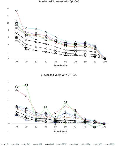
However, the cost mitigation benefits of NS do not translate to TE enhancements. If we compare the TE enhancements of IS in Figure 2 with the turnover and cost metrics in Figure 4, we find that the factor that benefits from the greatest enhancements in TE also suffers from the worst transaction costs (and vice versa). The factors with the highest relative turnover and eroded value (particularly EW, DRPW, MOM, QLTY, and DMV) enjoy the greatest TE benefits. This implies that the improvement in TE due to IS is not dependent on a factor’s turnover. Instead, industry coverage is more important.

We conclude that industry-based factor-replicating portfolio coverage, rather than cost reduction, is of primary importance when replicating factors with high fidelity. This insight represents an essential contribution to industry practice and the academic literature. Although cost reduction is a very important consideration in factor replication, when the primary goal is high-fidelity factor replication, replication strategies should also focus on high-fidelity returns rather than exclusively on cost mitigation.

Comparing IS with LP

So far, we have compared two stratification approaches, IS and NS. In this section, we consider a third, optimized portfolio stratification: LP. In theory, such optimization should substantially reduce factor replication TE, since (in contrast to IS and NS) the optimization’s explicit goal includes minimizing the TE. Ideally, LP provides optimized weights for a stratified factor portfolio that efficiently spans the complete benchmark (i.e., 100% stratification), generating high-fidelity tracking while reducing replication costs.

Motivated by the seminal study of Sharpe (1971), we focus on LP to find an optimized factor replication portfolio for EW.⁹ Crucially, in contrast to Rossbach and Karlow (2019), but similar to Stentoft and Wang (2019), we incorporate costs. Overtly incorporating factor rebalancing costs in the optimization is essential for realistic, practical factor replication. Akin to Stentoft and Wang (2019), we obtain optimized portfolio weights using the dual objective of minimizing both the after-cost TE and replication trading costs.

We compare the performance of each competing technique (i.e., IS, NS, and LP) in Figure 1 and Table 5.¹⁰ The “costed” LP optimal portfolio TE is illustrated in Figure 1.¹¹ Theoretically, LP minimizes the TE by finding a set of portfolio weights in the stratified portfolio that best span the complete factor benchmark, providing low-cost, efficient factor replication. Empirically, the TE of LP is slightly greater than for NS, leading to a positive and significant ΔTE value (statistical tests are relegated to Table C.1). This finding is in contrast to that of Table 3, where, for all factors, the TE of IS is always less than that of NS, resulting in a significant and negative ΔTE.

Table 5. QR1000 Dollar Ending Value ($) for EW Factor IS, NS, and LP by Stratification Percentage for Costless and Costed Portfolios

%	IS		NS		LP
Strat.	Costless EW ($)	Costed EW ($)	Costless EW ($)	Costed EW ($)	Costless EW ($)	Costed EW ($)
10%	$27.14	$17.98	$24.29	$17.25	$26.54	$18.54
40%	$31.84	$23.85	$30.20	$23.55	$29.79	$22.68
70%	$33.01	$24.60	$31.22	$23.90	$30.35	$22.22
100%	$31.05	$25.26	$31.05	$25.26	$34.95	$25.94

Notes: By design, linear programming (LP) should select investment weights for each stratified portfolio to reduce both tracking error (TE) and the costs of factor replication. Here, the costless ending value assumes no trading costs, whereas the costed results include turnover costs in forming the LP portfolio. LP delivers competitive dollar-ending value. Even though the LP 100% stratified portfolio, has a slightly larger TE (see Figure 1), it enjoys both the best costless and costed dollar ending value. No approach dominates across all stratifications.

The main reason LP generates inferior TE is its poor industry coverage. LP selects stratified portfolio weights to minimize TE and costs explicitly, but, in contrast to IS, LP does not explicitly maximize industry coverage. When we compare the analogous EW and LP DMRS regressions of Equation (4)(4) $$\Delta {TE}_{s,t}^{}\equiv {|TE}_{s,t}^{IS}\left|\mathrm{ }-{|TE}_{s,t}^{NS}\right|={\alpha }_s+b_s{{\mathit{RMRF}}_t^{\mathrm{*}}}_{}+s_s{{\mathit{SMB}}_t^{\mathrm{*}}}_{}+{h_s{{\mathit{HML}}_t^{\mathrm{*}}}_{}}_{}+r_s{{\mathit{RMW}}_t^{\mathrm{*}}}_{}{+{c_s{{\mathit{CMA}}_t^{\mathrm{*}}}_{}}_{}+i}_s\Delta {\mathit{ICI}}_{s,t}^{}+\mathrm{ }{ϵ}_{s,t}$$(4) in Panels A and B of Table 4, we find significant and relatively large ΔICI coefficients in Panel B for LP (between 6 and 10 times larger than EW), indicative of poor LP industry coverage, and thus responsible for the relatively poor TE that ensues. Ultimately, these results highlight how important industry coverage is for high-fidelity factor replication.

The IS, NS, and LP portfolio ending values are reported in Table 5. The dollar-ending value is the end value of an initial, one-dollar investment (see Table 1). Although both results utilize costs in LP, the costless ending value assumes no trading costs. We focus on the costed results as the true economic value of LP can only be ascertained after costs. By design, LP should select investment weights for each stratified portfolio to reduce both TE and the costs of factor replication. We see in Table 5 that LP delivers a competitive dollar-ending value, similar to IS and NS. Even though for LP, the 100% stratified portfolio has a larger TE (i.e., 13 basis points per month), it enjoys both the best costless and costed ending values. However, across all stratifications, no approach dominates. Ultimately, LP generates credible economic value, although LP is not comprehensively better than IS.

Economic Enhancement of Industry-Stratified Portfolios

Our goal is to ascertain the economic value of efficient, high-fidelity, after-cost factor replication using IS. Here, we clarify how the statistically significant improved IS TE translates to economic benefits for the factor investor.

In Table 3, we report the TE and ΔTE using IS and NS for various factors. We concluded that portfolio stratification could be an effective mechanism for promoting viable factor replication. However, ultimately, to understand the economic significance of IS, we must translate the statistically significant TE differences in Table 3 into economically meaningful results. To do so, as our economic measure, we take the dollar-ending value of our factor portfolio, which represents the value of a factor investment after 30 years. By construction, the costless factor benchmark has a dollar-ending value that is always higher than IS and NS. For brevity, in Table 6, we only report the difference (in millions of dollars) between the ending values of the IS and NS factor portfolios. Since these differences are often positive, it follows that IS tends to be closer to the benchmark ending values than NS.¹² This means that the lower IS TE from Table 3 translates to higher factor portfolio ending values, closer than NS to the costless benchmark. Given the initial $1 billion investment, the magnitude of the economic benefits of IS is large, often demonstrating enhancements worth hundreds of millions, and occasionally over a billion dollars. We conclude that IS translates to both statistically enhanced TEs (Table 3) and economically meaningful improvements (see Table 6) for factor replication.

Table 6. QR1000 Economic Significance ($millions) between IS and NS Portfolios

% Strat. /	FI	EW	DW-1	DW-2	DW-3	DRPW	DMV	MOM	QLTY
Factor
10%	$774	$712	$795	$839	$784	$608	$463	$713	$184
40%	−$121	$317	$252	$188	$108	$136	−$39	$474	−$954
70%	$197	$711	$532	$379	$187	$67	−$444	$227	$911

Notes: As our economic measure, we take the difference in dollar-ending value between industry (IS) and naively stratified (NS) portfolios, representing the value of a factor investment after 30 years given the initial $1 billion investment. We report the difference (in $millions of dollars) between the ending value of the IS and NS factor portfolios after costs at different stratification levels. We see that the magnitude of the economic benefits of industry stratification (IS) is large. Given the initial $1 bn investment, IS enhancements are often worth hundreds of millions of dollars. As these differences are often positive, IS tends to be closer to the benchmark ending values than NS.

Conclusion

To construct high-fidelity factor-replicating portfolios, we use a new IS approach that shares similar industry exposures to the factor benchmark but removes the costliest stock by industry in the replication portfolio. Our contribution theoretically motivates and empirically demonstrates the consistent benefits of our novel IS methodology for factor investing. We demonstrate the practical implications of our work and show significant economic enhancements.

Acknowledgements

The authors would like to thank Charles Custeau and Nick Diamidis for research assistance. We dedicate this work to the memory of Dr. Neil Burgess and Dr. Andrew Sanford.

Disclosure Statement

No potential conflict of interest was reported by the author(s).

Additional information

Notes on contributors

Surpreet Bharjana

Surpreet Bharjana is an Investment Analyst at Willis Towers Watson, Melbourne, Australia.

Rohan Fletcher

Rohan Fletcher is a Research Officer in the Department of Banking & Finance, Monash Business School, Monash University, Clayton, Victoria, Australia.

Paul Lajbcygier

Paul Lajbcygier is an Associate Professor in the Departments of Banking & Finance and Econometrics and Business Statistics, Monash Business School, Monash University, Clayton, Victoria, Australia.

Notes

1 This monthly reconstitution of the QR1000 generates greater turnover than the Russell 1000 index, since stocks enter and exit the QR1000 each month, not just on designated reconstitution days.

2 One reason for the success of IS is its reliance upon stable and consistent industry categorization. We acknowledge that potential look-ahead bias exists due to stocks allocated to industries ex post. This would be more pronounced for conglomerates. Since we consider the post-1990 period, we know that, after 1990, conglomerates narrowed their focus (see Online Supplemental Material Appendix C). Therefore, membership stability should be enhanced for our sample, and any potential bias should be reduced.

3 We use the one-way round-lot commission rates (sliding from 0.25% in 1987 to 0.10% in 2000) taken from Figure 3 of Jones (2002), which are consistent with those cited by Jones and Lipson (2001) and Keim and Madhavan (1998). After 2000, we assume that the commission rates stay constant at the 2000 rate of 0.10%. According to Chen et al. (2005), the commissions are small relative to the price impact costs for typical fund sizes. When index portfolio rebalancing occurs, the closing price on the last trading day of the month is used as the purchase or sale price, which has the advantageous property that, by definition, execution at this price will induce no index TE for the investor.

4 First, the performance metrics, which measure how well each factor portfolio performs with and without costs, are annualized geometric returns, annualized volatility, the “value of $1” (obtained at the end of the investment period), and the ratio to the benchmark (of the costly to the costless benchmark). Second, the turnover metrics, which measure how much the factor transacts, include annualized turnover and the “trade of $1” (dollars traded for each $1 invested). These metrics provide information about how much trading occurs to rebalance each factor and minimize TEs periodically. Third, the transaction cost metrics, which measure the implicit/explicit costs of trading for each factor, include the “cost of $1” (transaction costs per dollar), the “percentage of costless” (percentage remaining after the eroded value of trading is removed from the value of $1), and the eroded value (total dollar cost of trading). Finally, we include two measures of benchmark replication quality: the TE difference of the monthly benchmark and the information ratio (Goodwin, 1998).

5 This makes sense, since this portfolio comprises many smaller stocks, which, in contrast to MCWI, often have large investment weights. Thus, the industry bias induced by NS will be relatively large, resulting in a larger TE.

6 Given that the ICI has a zero lower bound (see Equation (4)) and that we calculate the difference in the ICI (i.e., ΔICI) between the IS and NS portfolios, a negative ΔICI value means that industry-stratified portfolios must be closer to the zero lower bound, which, in turn, means that they are closer to the benchmark index industry coverage.

7 The reason almost all the significant ΔICI coefficients are positive is that both the ΔICI coefficient and the dependent variable, ΔTE, are negative. In combination, these results mean that the ΔICI coefficient should be positive if IS leads to industry coverage closer to the benchmark and also generates lower TE to the benchmark.

8 The measures we use are the differences in Annual Turnover and Eroded Value between the IS and NS portfolios: ΔAnnual Turnover = Annual Turnover IS − Annual Turnover NS and ΔEroded Value = Eroded Value IS − Eroded Value NS. For each factor, the Annual Turnover and Eroded Value results are similar. This contrasts with Table 1, where the results apply only to 100% stratified costed and costless factor benchmarks. In addition, in Table 1, Annual Turnover and Eroded Value are reported, not ΔAnnual Turnover and ΔEroded Value.

9 We concentrate on the EW factor when applying LP stratification. EW represents an “extreme” factor portfolio as it requires very expensive portfolio turnover for high-fidelity replication. If for EW, we can obtain strong optimized replication (that reduces turnover while maintaining high-fidelity benchmark tracking), this suggests that optimization may also be useful for other factors. EW is also among the best-known of factors and easiest to implement with optimization.

10 The algorithm used for LP is provided in Figure C.1 of Online Supplemental Material Appendix C. In summary, a rolling window of 6 months is used to find the optimized LP weights, estimated in sample and applied in the next month out of sample. The TE and dollar-ending value are calculated using the weights found in sample on the out-of-sample month. The optimizer can select any weight for a stock. Any deviation from equal weighting generates a tracking cost. For all 6 months in sample, the weights for a stock must be the same.

11 In Figure 1, we see that the TE is never zero. This is because we include costs. Including costs must lead to a non-zero TE relative to the costless benchmark for all stratifications. Also, at 100% stratification, IS/NS and LP do not have identical TE. LP is greater than IS/NS TE at 100% stratification. This is to be expected, even though LP initiates its equal-weighted optimization with a replicating portfolio that uses the same stocks as NS. LP estimates the optimal investment weights using a historical, rolling 6-month window of these stock returns, which are then applied to the following month’s data to calculate the TE. Empirically, such portfolio optimization can be fraught (see Michaud 1989; Rossbach and Karlow 2019) as local minima may not be global (Appendix C, Section C.1). By contrast, IS finds investment weights by stratifying the portfolio using (stable) industry classification (see Section “ Portfolio Stratification Methodologies”). Furthermore, even at 100% stratification, LP may select optimal stock weights to be zero, leading to differences in stock lists and, ultimately, differences in TE between IS/NS and LP. Also, LP and IS portfolio constituent stock lists may differ due to monthly benchmark portfolio changes. Since the benchmark is reconstituted monthly, new stocks are added and old stocks are deleted in the following month. However, since many stocks in the historical window will not appear in the following month (and vice versa), this induces a tracking error for LP. In contrast, IS does not use a historical window to estimate investment weights and hence avoids this issue. Thus, in Figure 1, we observe a slight widening in the TE “spread” between IS and LP as the stratification percentage increases. This effect becomes more pronounced and the spread widens as the stratification percentage increases and more stocks are included/excluded each month.

12 The TE measure does not discriminate between lower or higher returns below or above the benchmark. By construction, the TE measure is indifferent to whether IS returns are above or below the benchmark. A lower IS TE does not guarantee a higher dollar-ending value for IS compared with NS.

References

- Ahn, D. H., J. Conrad, and R. F. Dittmar. 2009. “Basis Assets.” Review of Financial Studies 22 (12) :5133–5174. doi:10.1093/rfs/hhp065.
- Aked, M., and M. Moroz. 2013. The Market Impact of Index Rebalancing. Unpublished White Paper. Research Affiliates, Inc.
- Amihud, Y., and H. Mendelson. 1989. “The Effects of Beta, Bid-Ask Spread, Residual Risk, and Size on Stock Returns.” The Journal of Finance 44 (2): 479–486. doi:10.1111/j.1540-6261.1989.tb05067.x.
- Ang, A., L. Chen, M. Gates, and P. Henderson. 2021. “Index + Factors + Alpha.” Financial Analysts Journal 77 (4): 45–64. doi:10.1080/0015198X.2021.1960782.
- Arnott, R. D., J. Hsu, and P. Moore. 2005. “Fundamental Indexation.” Financial Analysts Journal 61 (2): 83–99. doi:10.2469/faj.v61.n2.2718.
- Arnott, R., C. R. Harvey, V. Kalesnik, and J. Linnainmaa. 2019. “Alice’s Adventures in Factorland: Three Blunders That Plague Factor Investing.” The Journal of Portfolio Management 45 (4): 18–36. doi:10.3905/jpm.2019.45.4.018.
- Baule, R. 2010. “Optimal Portfolio Selection for the Small Investor Considering Risk and Transaction Costs.” OR Spectrum 32 (1): 61–76. doi:10.1007/s00291-008-0152-5.
- Bhojraj, S., C. M. Lee, and D. K. Oler. 2003. “What’s My Line? A Comparison of Industry Classification Schemes for Capital Market Research.” Journal of Accounting Research 41 (5): 745–74. doi:10.1046/j.1475-679X.2003.00122.x.
- Cerniglia, J., and F. J. Fabozzi. 2018. “Academic, Practitioner, and Investor Perspectives on Factor Investing.” The Journal of Portfolio Management 44 (4): 10–16. doi:10.3905/jpm.2018.44.4.010.
- Chan, L. K., J. Lakonishok, and B. Swaminathan. 2007. “Industry Classifications and Return Comovement.” Financial Analysts Journal 63 (6): 56–70. doi:10.2469/faj.v63.n6.4927.
- Chen, A., and M. Velikov. 2022. “Zeroing in on the Expected Returns of Anomalies.” Journal of Financial and Quantitative Analysis: forthcoming 19 October 2021 1–26. doi:10.1017/S0022109022000874.
- Chen, Z., W. Stanzl, and M. Watanabe. 2005. Price Impact Costs and the Limit of Arbitrage. Working Paper. New Haven, CT: Yale School of Management.
- Clarke, R., H. de Silva, and S. Thorley. 2013. “Risk Parity, Maximum Diversification, and Minimum Variance: An Analytic Perspective.” The Journal of Portfolio Management 39 (3): 39–53. doi:10.3905/jpm.2013.39.3.039.
- Daniel, K., and S. Titman. 1997. “Evidence on the Characteristics of Cross Sectional Variation in Stock Returns.” The Journal of Finance 52 (1): 1–33. doi:10.1111/j.1540-6261.1997.tb03806.x.
- Daniel, K., L. Mota, S. Rottke, and T. Santos. 2020. “The Cross-Section of Risk and Returns.” The Review of Financial Studies 33 (5): 1927–79. doi:10.1093/rfs/hhaa021.
- DeMiguel, V., L. Garlappi, and R. Uppal. 2009. “Optimal Versus Naïve Diversification: How Inefficient is the 1/N Portfolio Strategy?” Review of Financial Studies 22 (5): 1915–1953. doi:10.1093/rfs/hhm075.
- Fama, E. F., and K. R. French. 2015. “A Five-Factor Asset Pricing Model.” Journal of Financial Economics 116 (1): 1–22. doi:10.1016/j.jfineco.2014.10.010.
- Fama, E., and K. French. 1993. “Common Risk Factors in the Returns on Stocks and Bonds.” Journal of Financial Economics 33 (1): 3–56. doi:10.1016/0304-405X(93)90023-5.
- Fernholz, R., R. Garvy, and J. Hannon. 1998. “Diversity-Weighted Indexing.” The Journal of Portfolio Management 24 (2): 74–82. doi:10.3905/jpm.24.2.74.
- Goodwin, T. H. 1998. “The Information Ratio.” Financial Analysts Journal 54 (4): 34–43. doi:10.2469/faj.v54.n4.2196.
- Hrazdil, K., K. Trottier, and R. Zhang. 2013. “A Comparison of Industry Classification Schemes: A Large Sample Study.” Economics Letters 118 (1): 77–80. doi:10.1016/j.econlet.2012.09.022.
- Jegadeesh, N., and S. Titman. 1993. “Returns to Buying Winners and Selling Losers: Implications for Stock Market Efficiency.” The Journal of Finance 48 (1): 65–91. doi:10.1111/j.1540-6261.1993.tb04702.x.
- Jones, C. M. 2002. “A Century of Stock Market Liquidity and Trading Costs.” Available at SSRN 313681.
- Jones, C., and M. Lipson. 2001. “Sixteenths: Direct Evidence on Institutional Trading Costs.” Journal of Financial Economics 59 (2): 253–78. doi:10.1016/S0304-405X(00)00087-8.
- Kacperczyk, M., C. Sialm, and L. Zheng. 2005. “On the Industry Concentration of Actively Managed Equity Mutual Funds.” The Journal of Finance 60 (4): 1983–2011. doi:10.1111/j.1540-6261.2005.00785.x.
- Keim, D. B., and A. Madhavan. 1998. “The Cost of Institutional Equity Trades.” Financial Analysts Journal 54 (4): 50–69. doi:10.2469/faj.v54.n4.2198.
- Larsen, G. A., and B. G. Resnick. 1998. “Empirical Insights on Indexing.” The Journal of Portfolio Management 25 (1): 51–60. doi:10.3905/jpm.1998.409656.
- Lewellen, J., S. Nagel, and J. Shanken. 2010. “A Skeptical Appraisal of Asset Pricing Tests.” Journal of Financial Economics 96 (2): 175–194. doi:10.1016/j.jfineco.2009.09.001.
- Maillard, S., T. Roncalli, and J. Teïletche. 2010. “The Properties of Equally Weighted Risk Contribution Portfolios.” The Journal of Portfolio Management 36 (4): 60–70. doi:10.3905/jpm.2010.36.4.060.
- Michaud, R. O. 1989. “The Markowitz Optimization Enigma: Is ‘Optimized’ Optimal?” Financial Analysts Journal 45 (1): 31–42. doi:10.2469/faj.v45.n1.31.
- Modigliani, F., and M. H. Miller. 1958. “The Cost of Capital, Corporation Finance and the Theory of Investment.” The American Economic Review 48 (3): 261–297.
- Novy-Marx, R., and M. Velikov. 2016. “A Taxonomy of Anomalies and Their Trading Costs.” The Review of Financial Studies 29 (1): 104–147.
- Novy-Marx, R., and M. Velikov. 2019. “Comparing Cost-Mitigation Techniques.” Financial Analysts Journal 75 (1): 85–102. doi:10.1080/0015198X.2018.1547057.
- Pham, M. C., H. N. Duong, and P. Lajbcygier. 2017. “A Comparison of the Forecasting Ability of Immediate Price Impact Models.” Journal of Forecasting 36 (8): 898–918. doi:10.1002/for.2405.
- Roll, R. 1992. “A Mean/Variance Analysis of Tracking Error.” The Journal of Portfolio Management 18 (4): 13–22. doi:10.3905/jpm.1992.701922.
- Ross, S. 1988. “Comment on the Modigliani–Miller Propositions.” Journal of Economic Perspectives 2 (4): 127–133. doi:10.1257/jep.2.4.127.
- Rossbach, P., and D. Karlow. 2019. “Structural Minimization of Tracking Error.” Quantitative Finance 19 (3): 357–366. doi:10.1080/14697688.2018.1527036.
- Rudd, A. 1980. “Optimal Selection of Passive Portfolios.” Financial Management 9 (1): 57–66. doi:10.2307/3665314.
- Rudolf, M., H. J. Wolter, and H. Zimmermann. 1999. “A Linear Model for Tracking Error Minimization.” Journal of Banking & Finance 23 (1): 85–103. doi:10.1016/S0378-4266(98)00076-4.
- Sharpe, W. F. 1971. “A Linear Programming Approximation for the General Portfolio Analysis Problem.” The Journal of Financial and Quantitative Analysis 6 (5): 1263–1275. doi:10.2307/2329860.
- Sloan, R. G. 1996. “Do Stock Prices Fully Reflect Information in Accruals and Cash Flows about Future Earnings?” Accounting Review 71 (3): 289–315.
- Stentoft, L., and S. Wang. 2019. “Consistent and Efficient Dynamic Portfolio Replication with Many Factors.” The Journal of Portfolio Management 46 (2): 79–91. doi:10.3905/jpm.2019.1.118.
- Van Montfort, K., E. Visser, and L. F. van Draat. 2008. “Index Tracking by Means of Optimized Sampling.” The Journal of Portfolio Management 34 (2): 143–52. doi:10.3905/jpm.2008.701625.