Predicting Corporate Bond Illiquidity via Machine Learning

Abstract

This paper tests the predictive performance of machine learning methods in estimating the illiquidity of US corporate bonds. Machine learning techniques outperform the historical illiquidity-based approach, the most commonly applied benchmark in practice, from both a statistical and an economic perspective. Gradient-boosted regression trees perform particularly well. Historical illiquidity is the most important single predictor variable, but several fundamental and return- as well as risk-based covariates also possess predictive power. Capturing nonlinear effects and interactions among these predictors further enhances forecasting performance. For practitioners, the choice of the appropriate machine learning model depends on the specific application.

Keywords:

• corporate bonds
• bond illiquidity
• quantitative credit research
• illiquidity forecasting
• machine learning

PL Credits: 2.0:

A growing strand of literature suggests that machine learning can enhance quantitative investing by uncovering exploitable nonlinear and interactive effects between predictor variables that tend to go unnoticed with simpler modeling approaches (see Blitz et al. 2023, for an excellent review of machine learning applications in asset management). The majority of these studies use machine learning techniques to predict stock returns, applying a large set of predictor variables. Most prominently, Gu, Kelly, and Xiu (2020) and Freyberger, Neuhierl, and Weber (2020) show that machine learning–based approaches outperform linear counterparts and generate remarkably high Sharpe ratios (of about 2 or even higher).¹ Bianchi, Büchner, and Tamoni (2021) and Bali et al. (2022) confirm the effectiveness of machine learning techniques in predicting government and corporate bond returns, respectively. Nevertheless, compared to the literature related to equities, machine learning applications in fixed-income research have received much less attention. This gap in the literature may be explained by the fact that our understanding of the risk–return tradeoff is still less developed in bond markets than in stock markets (Dickerson, Mueller, and Robotti 2023; Kelly, Palhares, and Pruitt 2023). We contribute to this recent literature by testing the predictive performance of machine learning methods in estimating the expected illiquidity of US corporate bonds.

In comparison to actively managed stock portfolios, there is limited alpha upside in a classical bond portfolio case, where individual bonds are bought as cheaply as possible and then often held until maturity (hoping that no default occurs). In this setup, every basis point in transaction cost savings is crucial for the success of such a strategy. Considering that corporate bonds are an asset class that is inherently plagued by illiquidity, the scarcity of work on predicting corporate bond illiquidity is surprising. Although the question of how to generate outperformance is the most important one for every investor, any outperformance potential depends on whether a seemingly superior trading strategy can be efficiently implemented in practice. Therefore, only a reliable estimate of a bond’s future liquidity enables an investor to assess whether this bond is priced in line with its fundamentals and to convert the return signals into a profitable investment strategy after accounting for transaction costs and other implementation frictions. Moreover, under the so-called SEC Liquidity Rule, accurate predictions of future bond liquidity are essential from a regulator’s and financial market supervision perspective to monitor bond funds' liquidity risk management.

The objective of our paper is to capture the rich facets of illiquidity in corporate bond markets using machine learning methods. Most studies that feature elements of bond illiquidity predictions rely on Amihud’s (2002) AR-1 approach (Bao, Pan, and Wang 2011; Friewald, Jankowitsch, and Subrahmanyam 2012; Dick-Nielsen, Feldhütter, and Lando 2012; Bongaerts, de Jong, and Driessen 2017). However, illiquidity, particularly in a complex market such as the one for corporate bonds, is multifaceted and incorporates a variety of market-specific factors and peculiarities (Sarr and Lybek 2002). Therefore, in addition to examining historical illiquidity, we consider a comprehensive set of bond characteristics and exploit their information content using machine learning models. We apply both relatively simple linear models (with and without penalty terms for multiple predictors) and more complex models that capture patterns of nonlinear and interactive effects in the relationship between predictor variables and expected bond illiquidity (such as regression tress and neural networks).² Another limitation in earlier work is that it considers mostly the bid–ask spread even if, in many cases, it is not a good representation of a bond trade’s realistic costs of execution. This is because the tradability of a bond itself and the market impact of the trade also have a substantial effect on investment performance. In our analysis, we use a large universe of US corporate bonds, three illiquidity measures that capture different aspects of illiquidity, a broad set of machine learning–based illiquidity estimators, and a comprehensive set of predictor variables based on historical illiquidity, fundamental predictors, return-based predictors, risk-based predictors, and macroeconomic indicators to uncover exploitable nonlinear and interactive patterns in the data.

Historical illiquidity is the most commonly used benchmark for predicting future bond illiquidity in the asset management industry. Examining level forecasts of illiquidity, our results confirm that machine learning–based prediction models that incorporate our comprehensive set of predictor variables outperform this popular benchmark. Tree-based models and neural networks, which additionally allow for nonlinearity and interaction effects, perform particularly well. For example, compared to the historical illiquidity benchmark, the average mean squared error (MSE) is more than 23% lower for neural networks. In a statistical sense, based on the Diebold and Mariano (1995) test, neural networks outperform the benchmark in more than 87% of the sample months. In addition, they are in the so-called model confidence set (Hansen, Lunde, and Nason 2011), that is, they are among the best-performing models that significantly dominate all other forecast models, more than six times as often. We attribute these improvements in prediction quality to the inclusion of slow-moving bond characteristics, such as age, size, and rating of a bond, as predictors as well as the ability of both tree-based models and neural networks to incorporate patters of nonlinearity and interactions in the relationship between expected illiquidity and these predictor variables. Furthermore, forecast errors of cross-sectional portfolio sorts indicate that the higher MSEs for the historical illiquidity benchmark describe a general pattern and are not driven by high forecast errors for only a few bonds with extreme characteristics.

In addition to analyzing the differences in level forecasts of illiquidity, we assess the economic value of illiquidity forecasts on the basis of a portfolio formation exercise, that is, by trading bonds sorted into portfolios based on realized and expected illiquidity. Compared to the historical illiquidity–based benchmark, machine learning forecast models are better at disentangling more liquid from less liquid bonds. Moreover, following Amihud and Mendelson (1986), investors should require higher expected returns for more illiquid bonds to compensate for higher trading expenses. Confirming this notion, we find that prediction models using machine learning techniques generate a higher illiquidity premium in the cross-section of bond returns than the historical illiquidity benchmark model. We highlight the economic value added in numerical examples and showcase that even small improvements in illiquidity estimates can result in large transaction cost savings, either directly in terms of a lower average bid–ask spread or indirectly in terms of a lower average price impact.

Furthermore, using relative variable importance metrics, we document that the historical illiquidity–based predictor is most important. This is because realized bond illiquidity is highly persistent and has long-memory properties. Among the remaining variables, fundamental and risk- as well as return-based covariates are the most important predictors (in that order). Macroeconomic indicators seem much less informative for future illiquidity. However, variable importance itself is also time-varying, and even predictors that are unconditionally less informative play important roles at times. Consequently, it is important to apply prediction models that are able to accommodate the time-varying nature of illiquidity indicators. By way of an example, we address this “black box” characteristic and illustrate how machine learning estimators for bond illiquidity generate value for investors. In particular, we visualize the combined effect of duration and rating on a bond’s illiquidity estimate, which confirms that a large part of the prediction outperformance of the more complex machine learning models is due to their ability to exploit nonlinear and interactive patterns.

Based on empirical evidence from predicting stock returns, several other recent papers take a more skeptical position on the use of machine learning in asset management applications. For example, Avramov, Cheng, and Metzker (2022) conclude that machine learning signals extract a large part of their profitability from difficult-to-arbitrage stocks (distressed stocks and microcaps) and during high limits-to-arbitrage market states (high–market volatility periods). Moreover, they document that machine learning–based performance will be even lower because of high turnover and trading costs. Similarly, Leung et al. (2021) show that the extent to which the statistical advantage of machine learning models can be translated into economic gains depends on the ability to take risk and implement trades efficiently.

Our work contributes to this strand of more critical work in the machine learning literature in two important ways. First, the low signal-to-noise ratio in stock returns typically leads to the risk of overfitting machine learning models. In contrast, bond liquidity, our variable of interest, is highly persistent, that is, past relations are more likely to continue to hold in the future, resulting in a higher signal-to-noise ratio. Therefore, machine learning methods should work at least as well or maybe even better for predicting future bond illiquidity than they do for predicting future stock and bond returns. Second, from a trading and execution perspective, a better representation of the expected illiquidity dimension in bond trading should provide economic value added for investors. Given the speed and complexity of bond trading, machine learning methods can help to exploit alpha signals even after accounting for transaction costs such that bond investors will embrace machine learning methods as an essential part of their trading practices in the future. Our results suggest that more complex machine learning models tend to be more powerful. However, because the implementation of these methods requires significant resources and skills, the choice of a specific type of prediction model will depend on how practitioners use illiquidity forecasts in their bond investment and trading decisions.

Literature Review

Previous literature documents that a bond’s illiquidity evolves throughout its lifetime (Warga 1992; Hong and Warga 2000; Hotchkiss and Jostova 2017), suggesting that dynamic estimation methods, such as the machine learning models we use, may be promising candidates for predicting bond illiquidity. Moreover, time-varying bond characteristics, such as size (Bao, Pan, and Wang 2011; Jankowitsch, Nashikkar, and Subrahmanyam 2011) and risk (Mahanti et al. 2008; Hotchkiss and Jostova 2017), impact expected bond illiquidity. Therefore, applying machine learning techniques, which adaptively incorporate these features along with their nonlinearities and interactions, should be valuable for predicting bond illiquidity.

Empirical evidence indicates that machine learning methods are able to outperform established approaches in various prediction tasks. Examples include forecasting stock returns (Gu, Kelly, and Xiu 2020; Freyberger, Neuhierl, and Weber 2020), predicting bond risk premiums (Bianchi, Büchner, and Tamoni 2021; Bali et al. 2022), and modeling stock market betas (Drobetz et al. 2024). Realized bond illiquidity, however, is much less noisy than realized stock and bond returns. Compared to return series but similar to beta variation, illiquidity is highly persistent over time. Given a higher signal-to-noise ratio, estimating future corporate bond illiquidity should provide a sensible use case for the application of machine learning techniques.

The study most closely related to our work is from Reichenbacher, Schuster, and Uhrig-Homburg (2020). They apply linear models to predict future corporate bond bid–ask spreads, which they use as their proxy for liquidity although it ignores the potentially large market impact of a trade. While these authors also use a large set of predictor variables and analyze their importance, they do not explore patterns of nonlinear and interactive effects in the relation between predictor variables and bond illiquidity estimates. In our own analysis, we extend their insightful work in several directions. Most important, (1) we compare the predictive performance of machine learning estimators to that of the commonly used historical illiquidity benchmark, (2) we analyze how machine learning models outperform by assessing forecast errors of cross-sectional portfolio sorts, (3) we use a comprehensive set of liquidity measures that also captures a bond trade’s market impact, (4) we assess the economic value added of machine learning–based estimators, and (5) we scrutinize the importance of nonlinear and interactive effects in establishing illiquidity predictions.

Our paper is related to recent studies that use machine learning in various fixed-income applications. For example, Fedenia, Nam, and Ronen (2021) show that random forest algorithms can be used to uncover a better trade signing model in the corporate bond market, that is, to determine whether a trade is buyer- or seller-initiated, which helps bond traders to better understand market dynamics and price behavior. Cherief et al. (2022) apply random forests and gradient-boosted regression trees to capture nonlinearities and interactions between traditional risk factors in the credit space. Their model outperforms linear pricing models in forecasting credit excess returns. Kaufmann, Messow, and Vogt (2021) use gradient-boosted regression trees to model the equity momentum factor (in addition to classical bond market factors such as size and illiquidity) in the corporate bond market.

Data

Following Bessembinder, Maxwell, and Venkataraman (2006), who emphasize the importance of using Trade Reporting and Compliance Engine (TRACE) transaction data, our empirical analysis is based on intraday transaction records for the US corporate bond market reported in the enhanced version of TRACE for the sample period from July 2002 to December 2020. The TRACE dataset comprises the most comprehensive information on US corporate bond transactions, with intraday observations on price, transaction volume, and buy and sell indicators.³ In addition, bond characteristics (issue information) such as bond type, offering and maturity dates, coupon specifications, outstanding amount, rating, and issuer information come from Mergent FISD.⁴

To clean the TRACE dataset, we use Dick-Nielsen’s (2009, 2014) procedure to remove duplicate, cancelled, and corrected entries. Following Bali, Subrahmanyam, and Wen (2021), we omit bonds from the sample that (1) are not listed or traded in the US public market; (2) are backed with a guarantee or linked to an asset; (3) have special features (perpetuals, convertible and puttable bonds, or floating coupon rates); or (4) have less than one year to maturity or are defaulted. For the intraday records, we eliminate transactions that (5) are labeled as when-issued or locked-in or have special sales conditions; (6) have more than a three-day settlement; and (7) have a volume less than $10,000 or a price less than $5.

Based on the intraday bond transaction records, we aggregate our database on a monthly basis and construct three distinct illiquidity measures that capture different aspects of illiquidity. All variables used in our empirical analyses are described in Table 1. First, we consider the transaction volume ($t\_\mathit{\text{volum}}{e}_t$), which is related to the capacity of actually trading the respective bond: (1) $$t\_\mathit{\text{volum}}{e}_t=\sum _{d=1}^{N_t}{Q}_d,$$(1) where $Q_d$ is the dollar trading volume on day $d$, and $N_{\mathrm{t}}$ is the number of trading days with positive-trading volume in each month $t.$ Second, following Hong and Warga (2000) and Chakravarty and Sarkar (2003), we compute the difference between the average customer buy and the average customer sell price on each day within a given month $t$ ($t\_\mathit{\text{sprea}}{d}_t$) to quantify transaction costs: (2) $$t\_\mathit{\text{sprea}}{d}_t=\frac{1}{N_t}{\sum }_{d=1}^{N_t}\frac{\overline{P_d^{\mathit{\text{Buy}}}}-\overline{P_d^{\mathit{\text{Sell}}}}}{0.5\times (\overline{P_d^{\mathit{\text{Buy}}}}+\overline{P_d^{\mathit{\text{Sell}}}})},$$(2) where $P_d^{\mathit{\text{Buy}}/\mathit{\text{Sell}}}$ is the average price of customer buy/sell trades on day $d.$ Third, we use Amihud’s (2002) measure of illiquidity ($\mathit{\text{amihu}}{d}_t$), which captures the aggregate price impact in each month $t:$ (3) $$\mathit{\text{amihu}}{d}_t=\frac{1}{N_t}\sum _{d=1}^{N_t}\frac{\left|r_d\right|}{Q_d}\times {10}^6,$$(3) where $r_d=\frac{P_{i,t}}{P_{i,t-1}}-1$ is a bond’s price return on day d.⁵

Table 1. Variable Descriptions and Definitions

#	Predictor	Description	Definition
Predictors based on historical illiquidity
1a	t_volume_hist	Historical transaction volume	Log historical transaction volume (computed as the average over the last 12 months)
1b	t_spread_hist	Historical transaction cost	Log historical transaction cost (computed as the average over the last 12 months)
1c	amihud_hist	Historical price impact	Log historical price impact (computed as the average over the last 12 months)
Fundamental predictors
2	age	Age	Bond age since first issuance, measured in number of years
3	size	Size	Log bond amount outstanding
4	rating	Rating	Numerical bond rating calculated as described in Bali et al. (2020), measured from 1 (good) to 22 (bad)
5	mat	Maturity	Time to maturity, measured in number of years
6	yield	Yield	Bond yield to maturity
7	dur	Duration	Bond price sensitivity to interest rate changes, measured in number of years
Return-based predictors
8	rev	Short-term reversal	Excess return in the prior month
9	mom	Momentum	Excess return from month −12 to month −1
10	ltr	Long-term reversal	Excess return from month −36 to month −1
11	vol	Volatility	Standard deviation, estimated from monthly returns over the last three years
12	skew	Skewness	Skewness, estimated from monthly returns over the last three years
13	kurt	Kurtosis	Kurtosis, estimated from monthly returns over the last three years
Risk-based predictors
14	var10	Value at Risk	Value at risk at the 10% level, measured as fourth lowest monthly return observation over the last three years
15	es10	Expected Shortfall	Expected shortfall at the 10% level, measured as average of the four lowest monthly return observations over the last three years
16	beta	Systematic risk	Bond market beta, measured as regression coefficient from the time-series ordinary least squares regression of monthly bond excess returns on market excess returns over the last three years
17	idio	Idiosyncratic risk	Idiosyncratic bond risk, measured as mean squared error of the residuals from the time-series ordinary least squares regression of monthly bond excess returns on market excess returns over the last three years
Macroeconomic indicators
18	dfy	Default spread	Yield differential between Moody’s Baa- and Aaa-rated corporate bonds

Notes: This table shows descriptions and definitions for each of the 18 bond illiquidity predictors used in the empirical analysis. The baseline sample includes intraday transaction records for the US corporate bond market reported in the enhanced version of TRACE for the sample period from July 2004 to November 2020.

Table 2 presents cross-sectional and time-series correlations of these three realized bond illiquidity measures. Panel A (cross-sectional) contains the time-series averages of monthly cross-sectional correlations, and Panel B (time-series) the cross-sectional averages of time-series correlations. The correlations (in absolute values) are far from perfect and range widely between −0.63 and +0.25, confirming that our three measures capture different aspects of illiquidity.

Table 2. Cross-Sectional and Time-Series Correlations between Illiquidity Measures

	Panel A: Cross-sectional			Panel B: Time-series
	t_volume	amihud	t_spread	t_volume	amihud	t_spread
t_volume	1.00	−0.63	−0.09	1.00	−0.41	0.06
amihud		1.00	0.42		1.00	0.25
t_spread			1.00			1.00

Notes: This table shows cross-sectional and time-series correlations among the three realized bond illiquidity measures, t_volume, amihud, and t_spread. Panel A (cross-sectional) contains the time-series averages of monthly cross-sectional correlations, and Panel B (time-series) the cross-sectional averages of time-series correlations. The baseline sample includes intraday transaction records for the US corporate bond market reported in the enhanced version of TRACE for the sample period from July 2004 to November 2020.

Based on monthly sortings of bonds into illiquidity deciles, Table 3 presents the average transition probabilities (together with one-sided t-statistics) for the three bond illiquidity measures. To keep the table tractable, we only show the diagonal elements of the full transition matrix, that is, the average probabilities to remain in the same illiquidity decile in the subsequent month. These “no-transition” probabilities all exceed 10%, confirming that bond illiquidity is persistent (Chordia, Sarkar, and Subrahmanyam, 2005; Acharya, Amihud, and Bharath, 2013) and suggesting that lagged historical illiquidity will be a particularly important predictor variable for expected illiquidity.

Table 3. Transition Probabilities

		Decile
		1	2	3	4	5	6	7	8	9	10
t_volume	Prob (no transition), %	45.75	28.70	22.26	19.16	17.39	17.00	17.62	20.70	29.22	62.47
	t value	88.54	82.57	59.91	53.58	46.53	40.05	48.96	54.94	76.65	168.25
amihud	Prob (no transition), %	37.03	19.47	15.75	13.79	13.61	13.31	13.85	14.86	17.65	25.06
	t value	39.89	37.68	35.76	26.75	28.13	23.42	25.85	30.52	44.71	51.87
t_spread	Prob (no transition), %	27.54	23.40	19.10	17.10	16.14	15.90	16.86	18.88	23.91	43.15
	t value	60.37	59.54	50.36	40.81	36.50	36.70	39.11	42.52	63.83	78.33

Notes: Based on monthly sortings of bonds into illiquidity deciles, this table shows average transition probabilities (together with one-sided t-statistics) for all three realized bond illiquidity measures (t_volume, amihud, and t_spread). Only the diagonal elements of the full transition matrix are shown, that is, the average probabilities to remain in the same illiquidity decile in the subsequent month (“no-transition” probabilities). The baseline sample includes intraday transaction records for the US corporate bond market reported in the enhanced version of Trade Reporting and Compliance Engine (TRACE) for the sample period from July 2004 to November 2020.

In addition to a predictor based on realized illiquidity over the past year that captures the time-series dynamics in illiquidity, we select from Bali, Subrahmanyam, and Wen (2021) a comprehensive set of 18 forecasting variables, which are described in Table 1. These variables capture basic return and risk characteristics of bonds.⁶ While these variables describe the characteristics of bonds in general and are somehow natural candidates for our forecasting task, they need not even be the best predictors for expected bond illiquidity. Our set of predictor variables includes six fundamental predictors based on the characteristics of bonds (age, size, rating, maturity, duration, and yield). In addition, it contains 10 technical indicators based on the historical bond return distribution, relating to return characteristics (short-term reversal, momentum, long-term reversal, volatility, skewness, and kurtosis) and risk characteristics (value-at-risk, expected shortfall, systematic risk, and idiosyncratic risk). Technical indicators are computed based on monthly excess bond returns: (4) $$r_{i,t}=R_{i,t}-r_{f,t}=\left(\frac{P_{i,t}+A{I}_{i,t}+C_{i,t}}{P_{i,t-1}+A{I}_{i,t-1}}-1\right)-r_{f,t},$$(4) where $P_{i,t}$ is the transaction price, $A{I}_{i,t}$ is the accrued interest, and $C_{i,t}$ is the coupon payment, if any, of bond $i$ in month $t.$ Based on the TRACE records, we first calculate the daily clean price as the transaction volume-weighted average of intraday prices to minimize the effect of bid–ask spreads in prices, following Bessembinder et al. (2009), and then convert the bond prices from daily to monthly frequency by keeping the price at the end of a given month $t.$ $r_{f,t}$ is the risk-free rate proxied by the US Treasury bill rate. If necessary, the value-weighted portfolio of all bonds serves as the proxy for the market portfolio. Finally, our analysis includes the default spread as the only macroeconomic covariate.

We only include a bond in our empirical analysis for month $t$ if the illiquidity measure under investigation is available and the bond provides complete information on all predictor variables, that is, there are no missing values. In every month, we require at least 100 bonds to be included in the cross-section. This limits our sample period to July 2004 through November 2020. The average monthly cross-section consists of 4,330 bonds for t_volume, 3,556 bonds for t_spread, and 4,328 bonds for amihud.

As in Cosemans et al. (2016), we winsorize outliers in both the illiquidity measures and all predictors (except the default spread) to the 1st and 99th percentile values of their cross-sectional distributions. Moreover, we correct for skewness in distributions by logarithmically transforming the three illiquidity measures and some of the predictor variables (see Table 1). Some predictors are constructed similarly—for example, value-at-risk and expected shortfall—or incorporate similar information—for example, maturity and duration—which leads to relatively high correlations. However, according to Lewellen (2015), multicollinearity is not a main concern in our setup because we are mostly interested in the overall predictive power of machine learning–based models rather than the marginal effects of each single predictor. Machine learning methods are suitable for solving the multicollinearity problem either by nature (tree-based models) or by applying different types of regularization, for example, a lasso-based penalization of the weights (neural networks).

Forecast Models

General Approach

Our objective is to examine whether machine learning methods outperform the historical illiquidity benchmark model, that is, the naïve rolling-window approach, in terms of predictive performance and, if yes, why. We are particularly interested in examining whether (1) incorporating our large set of bond characteristics as predictors and (2) allowing for nonlinearity and interactions in the relationship between these predictors and future (expected) illiquidity can add incremental predictive power. We run a horse race between the benchmark model that uses historical illiquidity (the average illiquidity over the last 12 months) and linear as well as nonlinear machine learning–based prediction models that exploit additional cross-sectional information, comparing their performance from both a statistical and an economic perspective. In addition, we analyze the characteristics and functioning scheme of the machine learning techniques that help explain their superior predictive performance.

Following the approach used for estimating market betas in Cosemans et al. (2016) and Drobetz et al. (2024), the estimation setting in our empirical tests is as follows: Out-of-sample illiquidity estimates are obtained at the bond level and on a monthly basis, following an iterative procedure. In the first iteration step, we use data up to the end of month $t$ and obtain forecasts for each bond $i$’s average monthly illiquidity during the out-of-sample forecast period (from the beginning of month $t+1$ to the end of month $t+k$), denoted as $I_{i,t+k|t}^F$ (or abbreviated $I_{i,t}^F$). We set $k$ equal to 12, focusing on a one-year forecast horizon.⁷ In the next iteration step, we use data up to the end of month $t+1$ and obtain forecasts of bond-level illiquidity during the subsequent out-of-sample forecast period (from the beginning of month $t+1+1$ to the end of month $t+1+k$). By iterating through the entire sample, we obtain time-series of overlapping annual out-of-sample illiquidity predictions, which we compare to realized illiquidity.

Next, we introduce the different models used to predict future bond illiquidity. Online Supplemental Appendix A provides details. While they differ in their overall approach and complexity, all models aim to minimize the forecast error of level predictions, defined as the MSE at the end of each month $t:$ (5) $${\mathit{\text{MSE}}}_{t+k|t}=\sum _{i=1}^{N_t}{{(I}_{i,t+k}^R-I_{i,t+k|t}^F)}^2,\text{with}k=12,$$(5) where $I_{i,t+k}^R$ is bond $i$’s realized average monthly illiquidity during the out-of-sample period (i.e., from the beginning of month $t+1$ to the end of month $t+k$), and $N_t$ is the number of bonds at the end of month $t.$

Benchmark Estimator

Most academic papers that focus on the bond market use a bond’s historical illiquidity as a naïve prediction for future illiquidity (Bao, Pan, and Wang 2011; Friewald, Jankowitsch, and Subrahmanyam 2012; Dick-Nielsen, Feldhütter, and Lando 2012; Bongaerts, de Jong, and Driessen 2017). Given the high persistence in realized bond illiquidity (see Table 2), we implement this naïve estimator in all our empirical tests. Since we focus on a one-year forecast horizon, we use the average monthly illiquidity over the last 12 months ($t\_\mathit{\text{volume}}\_\mathit{\text{hist}},$ $t\_\mathit{\text{spread}}\_\mathit{\text{hist}},$ and $\mathit{\text{amihud}}\_\mathit{\text{hist}}$) as our benchmark, thereby increasing the signal-to-noise ratio relative to the current-month illiquidity.

Machine Learning Estimators

Rather than simply averaging historical illiquidity measures, machine learning techniques focus explicitly on the objective of forecasting corporate bond illiquidity. Realized illiquidity enters our regressive framework as the dependent variable, while historical illiquidity, a set of bond characteristics, and macroeconomic indicators serve as predictors. We adapt the additive prediction error model from Gu, Kelly, and Xiu (2020) to describe a bond’s illiquidity: (6) $$I_{i,t+k}^R=E_t\left(I_{i,t+k}^R\right)+{\epsilon }_{i,t+k},$$(6) where $I_{i,t+k}^R$ is bond $i$’s realized illiquidity over the one-year forecast horizon starting at the beginning of month $t+1.$ Expected illiquidity is estimated as a function of multiple predictor variables and described by the “true” model $g^{\mathrm{*}}\left(z_{i,t}\right),$ where $z_{i,t}$ represents the P-dimensional set of predictors: (7) $$E_t\left(I_{i,t+k}^R\right)=g^{\mathrm{*}}\left(z_{i,t}\right).$$(7) Although our machine learning–based forecast models belong to different families (linear regressions, tree-based models, and neural networks), they are all designed to approximate the true forecast model by minimizing the out-of-sample MSE. Approximations of the conditional expectations $g^{\mathrm{*}}\left(z_{i,t}\right)$ are flexible and family-specific. Approximation functions $g\left(.\right)$ can be linear or nonlinear. Moreover, they can be parametric, with $g\left(z_{i,t},\theta \right),$ where $\theta$ is the set of true parameters, or nonparametric, with $g\left(z_{i,t}\right).$

A general problem is that machine learning methods are prone to overfitting, which is why we must control for the degree of model complexity by tuning the relevant hyperparameters. To avoid overfitting and maximize out-of-sample predictive power, the hyperparameters should not be preset, but rather must be determined adaptively from the sample data. We follow Gu, Kelly, and Xiu’s (2020) time-series cross-validation approach to fit the machine learning–based forecast models so that they produce reliable out-of-sample predictive performance. Online Supplemental Appendix A provides details on how we split the sample into three subsamples: a training sample, a validation sample, and a test sample. We obtain our first illiquidity estimates in June 2011, using six years of data for training and validation (2004:07–2009:06 and 2009:07–2010:06, respectively), which we then compare to the bonds’ realized illiquidity over the next year.⁸ This approach ensures that our test sample is truly out-of-sample, enabling us to evaluate a model’s out-of-sample predictive power. In total, we exploit eight years and six months of data for testing (up to the end 2019:11).

As already explained, we consider a set of 18 predictor variables (predictors based on historical illiquidity, fundamental predictors, return-based predictors, risk-based predictors, and macroeconomic indicators; see Table 1 for more details) to fit the machine learning techniques. We test three different forecast model families, which differ in their overall approach and complexity. Online Supplemental Appendix A provides more details on these techniques and how we implement them.

The first model family consists of linear regressions, for which we use the training sample to run pooled ordinary least squares regressions of future realized illiquidity $I_{i,t+k}^R$ on the set of 18 predictors. We either use the ordinary least squares loss function (lm) or modify it by incorporating a penalty term, that is, we apply an elastic net penalization (elanet). The latter is the most common machine learning technique to overcome the overfitting problem in high-dimensional regressions, for example, when the number of predictors becomes large relative to the number of observations. If not explicitly included as predetermined terms, pooled regressions (simple or penalized models) cannot capture nonlinear or interactive effects.

The second model family consists of tree-based models, for which we use random forests (rf) and gradient-boosted regression trees (gbrt), the most common models within this category. Finally, the third model family comprises neural networks (nn_1–nn_5), for which we consider specifications with up to five hidden layers and 32 neurons.⁹ Both tree-based models and neural networks incorporate nonlinearities and multiway interactions inherently, without the need to add new predictors to capture these effects.

Empirical Results

Having introduced the benchmark and machine learning–based estimation approaches, we now apply these models to forecast out-of-sample bond illiquidity. We focus on the amihud measure in presenting and discussing the empirical results going forward because what matters most to investors is the actual price impact their trades will have. The return premium associated with this illiquidity measure is generally considered an illiquidity risk premium that compensates for price impact or transaction costs. Our results are qualitatively similar for the alternative t_volume and t_spread measures. Supplementary Appendix C presents our main results using these two bond illiquidity measures together with other robustness tests.

We start with studying the models’ ability to predict bond illiquidity from a statistical perspective. Our focus is on the question whether machine learning–based level forecasts of illiquidity outperform the historical illiquidity benchmark. We assess the cross-sectional and time-series properties of our models’ prediction performance, particularly comparing the resulting forecast errors. We also investigate the underlying causes of differences in predictive performance by analyzing the forecast errors of cross-sectional portfolio sorts. Moreover, we evaluate whether differences in statistical predictive performance translate into economic gains in a portfolio formation exercise.

Cross-Sectional and Time-Series Properties of Illiquidity Estimates

To begin, we investigate the properties of illiquidity predictions obtained from the different forecast models.¹⁰ Panel A in Table 4 focuses on the cross-sectional properties, presenting the time-series means of monthly (1) cross-sectional averages of expected illiquidity, (2) cross-sectional standard deviations, and (3) cross-sectional minimum, median, and maximum values. Following Pástor and Stambaugh (1999), we report the implied cross-sectional standard deviation of true illiquidity, $\widehat{\mathit{\text{Std}}}\left(I^R\right)={\left[\overline{\mathit{\text{Var}}\left(I^F\right)}-{\overline{\widehat{\mathit{\text{Var}}}}}_{I_i^R}\right]}^{1/2},$ which helps to measure an illiquidity forecast’s precision. The minuend $\overline{\mathit{\text{Var}}\left(I^F\right)}$ is the time-series average of monthly cross-sectional variances, and the subtrahend ${\overline{\widehat{\mathit{\text{Var}}}}}_{I_i^R}$ denotes the cross-sectional average of bonds’ sampling variance. Small gaps between observed and implied standard deviations imply small estimation errors, indicating measurement of true illiquidity with high precision. Panel B focuses on time-series properties, presenting the cross-sectional means of (1) time-series averages of estimated illiquidity; (2) time-series standard deviations; (3) time-series minimum, median, and maximum values; and (4) first-order autocorrelations.

Table 4. Cross-Sectional and Time-Series Properties of Illiquidity Estimates

	Panel A: Cross-sectional						Panel B: Time-series
	Mean	SD	Min	Median	Max	Impl. SD	Mean	SD	Min	Median	Max	Autocorr.
hist	−4.77	0.59	−6.97	−4.67	−3.80	0.49	−4.79	0.29	−5.45	−4.77	−4.30	0.91
lm	−4.78	0.43	−6.45	−4.72	−3.73	0.39	−4.80	0.18	−5.22	−4.79	−4.49	0.91
elanet	−4.77	0.42	−6.39	−4.71	−3.77	0.38	−4.79	0.17	−5.17	−4.78	−4.49	0.91
rf	−4.78	0.42	−6.72	−4.67	−4.09	0.39	−4.80	0.16	−5.16	−4.78	−4.54	0.90
gbrt	−4.77	0.43	−6.84	−4.66	−3.93	0.39	−4.79	0.17	−5.19	−4.77	−4.50	0.88
nn_1	−4.79	0.43	−6.84	−4.69	−3.90	0.38	−4.80	0.18	−5.23	−4.78	−4.50	0.92

Notes: Properties of out-of-sample bond illiquidity estimates (the average monthly amihud measure) are obtained from the different forecast models (hist, lm, elanet, rf, gbrt, and nn_1). Panel A focuses on cross-sectional properties, presenting time-series means of (1) the value-weighted cross-sectional average of estimated bond liquidity, (2) the cross-sectional standard deviation, and (3) the cross-sectional minimum, median, and maximum value. Following the procedure outlined in Paster and Stambough (1999), it also reports the implied cross-sectional standard deviation of true bond illiquidity, that is, $\widehat{\mathit{\text{Std}}}\left(I^R\right)={\left[\overline{\mathit{\text{Var}}\left(I^F\right)}-{\overline{\widehat{\mathit{\text{Var}}}}}_{I_i^R}\right]}^{1/2 }.$ Panel B focuses on time-series properties, presenting value-weighted cross-sectional means of (1) the time-series average of bond illiquidity’ (2) the time-series standard deviation; (3) the time-series minimum, median, and maximum value; and (4) the first-order autocorrelation. Following Becker et al. (2021), firms with fewer than 50 bond illiquidity estimates are omitted for the summary statistics in Panel B. The baseline sample includes intraday transaction records for the US corporate bond market reported in the enhanced version of Trade Reporting and Compliance Engine (TRACE) for the sample period from July 2004 to November 2020.

The cross-sectional and time-series means for each estimation approach are close to those for realized illiquidity,¹¹ while the cross-sectional and time-series dispersions vary across the models. Standard deviations (SDs) are greatest for the hist model, which uses only time-series information based on a bond’s historical illiquidity. This restriction leads to extreme and highly volatile illiquidity estimates. In contrast, incorporating cross-sectional information about a bond’s characteristics, its return-risk profile, and macroeconomic indicators reduces the cross-sectional and time-series standard deviations in expected illiquidity notably. Since this reduction in volatility is similar for all machine learning models, it seems to be the inclusion of slow-moving bond characteristics as predictors in the additive prediction error model rather than the ability of the more complex models to capture nonlinearity and interactions that results in less extreme and less volatile estimates. In other words, the time variation in bond characteristics is able to pick up long-run movements in illiquidity.

The observed cross-sectional SD of illiquidity forecasts in Panel A is most informative for the assessment of a model’s precision when comparing it to the implied cross-sectional standard deviation of true illiquidity (Impl. SD). This comparison reveals that true illiquidity is measured with the lowest precision (implying larger gaps between observed and implied SDs) by the historical illiquidity–based benchmark model and with the highest precision (implying smaller gaps) by the machine learning–based models. For example, the difference between SD and Impl. SD is 0.1 for the hist model and only 0.05 for the nn_1 model. Finally, although they incorporate slow-moving bond characteristics as predictors, the average time-series autocorrelations of machine learning–based models in Panel B are similar to that of the historical illiquidity benchmark model (all around 0.90).

Average Forecast Errors and Forecast Errors over Time

Next, we examine the statistical predictive performance of the different forecast models by comparing their forecast errors. Panel A of Table 5 reports the time-series means of monthly MSEs (based on a one-year forecast horizon), calculated as specified in Equation (5)(5) $${\mathit{\text{MSE}}}_{t+k|t}=\sum _{i=1}^{N_t}{{(I}_{i,t+k}^R-I_{i,t+k|t}^F)}^2,\text{with}k=12,$$(5) . Exploiting only bond-level time-series information, the estimates based on historical illiquidity generate sizable forecast errors (0.192 in the hist model). Incorporating cross-sectional information reduces the average MSE noticeably. Linear regressions (both simple and penalized, with MSEs of 0.160 and 0.157, respectively) reduce the average forecast error relative to the hist model by around 18%. Inspecting nonlinear machine learning methods, we find that tree-based models and neural networks reduce the average forecast error relative to linear regressions even further (with average MSEs of 0.145, 0.144, and 0.147 for the rf, gbrt, and nn_1 model, respectively). Tree-based models and neural networks perform similarly well, decreasing the average forecast error relative to the historical illiquidity–based benchmark by more than 23%. We conclude that these models’ ability to capture nonlinearity and interactions further enhances the quality of illiquidity predictions by reducing the forecast error of level predictions.

Table 5. Forecast Errors

	Forecast model
	hist	lm	elanet	rf	gbrt	nn_1
Panel A: Average forecast errors
MSE	0.192	0.160	0.157	0.145	0.144	0.147
Panel B: Forecast errors over time
In MCS	0.00	2.94	7.84	51.96	74.51	50.98
vs. hist		92.16	98.04	94.12	99.02	94.12
vs. lm	1.96		40.20	88.24	86.27	87.25
vs. elanet	0.00	19.61		83.33	79.41	77.45
vs. rf	0.00	2.94	6.86		46.08	22.55
vs. gbrt	0.00	0.00	2.94	14.71		17.65
vs. nn_1	1.96	5.88	10.78	30.39	46.08
T	102	102	102	102	102	102

Notes: This table presents differences in forecast errors for the amihud illiquidity measure produced by the forecast models (hist, lm, elanet, rf, gbrt, and nn_1). Panel A reports the time-series means for monthly value-weighted mean-squared errors (MSEs), that is, ${\mathit{\text{MSE}}}_{t+k|t}={\sum }_{i=1}^{N_t}{w}_{i,t}{{(I}_{i,t+k}^R-I_{i,t+k|t}^F)}^2,$ with $k=12,$ where $N_t$ is the number of bonds in the sample at the end of month $t.$ Panel B reports the fraction of months during the out-of-sample period for which the column model is (1) in the Hansen, Lunde, and Nason (2011) model confidence set (MCS) and (2) significantly better than the row model in a pairwise comparison (according to Diebold and Mariano (1995) test [DM test] statistics). The DM tests of equal predictive ability inspect differences in stock-level squared forecast errors (SEs), that is, $S{E}_{i,t+k|t}={{(I}_{i,t+k}^R-I_{i,t+k|t}^F)}^2,$ with $k=12.$ The DM test statistic in month $t$ for comparing the model under investigation $j$ with a competing model $i$ is $D{M}_{\mathit{\text{ij}},t}=\frac{{\overline{d}}_{\mathit{\text{ij}},t}}{{\widehat{\sigma }}_{{\overline{d}}_{\mathit{\text{ij}},t}}},$ where $d_{\mathit{\text{ij}},t}=S{E}_{i,t+k|t}-S{E}_{j,t+k|t}$ is the difference in SEs, ${\overline{d}}_{\mathit{\text{ij}},t}={\sum }_{i=1}^{N_t}{d}_{\mathit{\text{ij}},t}$ is the cross-sectional average of these differences, and ${\widehat{\sigma }}_{{\overline{d}}_{\mathit{\text{ij}},t}}$ is the Newey and West (1987) estimator with four lags to account for possible heteroskedasticity and autocorrelation. Positive signs of $D{M}_{\mathit{\text{ij}},t}$ indicate superior predictive performance of model $j$ relative to model $i$ in month $t,$ that is, that model $j$ yields, on average, lower forecast errors than model $i.$ All statistical tests are based on the 5% significance level. The baseline sample includes intraday transaction records for the US corporate bond market reported in the enhanced version of Trade Reporting and Compliance Engine (TRACE) for the sample period from July 2004 to November 2020.

Since, by construction, these figures reflect a forecast model’s average predictive performance, we next investigate the forecast errors over time. Panel B of Table 5 reports the fraction of months during the out-of-sample period for which the column model (1) is in the Hansen, Lunde, and Nason (2011) model confidence set (MCS) and (2) is significantly better than the row model in a pairwise comparison (according to Diebold and Mariano (1995) test [DM test] statistics). The MCS approach incorporates an adjustment for multiple testing and is designed to include the best forecast model(s) based on a certain confidence level.¹² The DM test of equal predictive ability inspects pairwise differences in bond-level squared forecast errors (SEs): (8) $$S{E}_{i,t+k|t}={{(I}_{i,t+k}^R-I_{i,t+k|t}^F)}^2,\text{with}k=12.$$(8) The DM test statistic in month $t$ for comparing model $j$ with a competing model $i$ is $D{M}_{\mathit{\text{ij}},t}=\frac{{\overline{d}}_{\mathit{\text{ij}},t}}{{\widehat{\sigma }}_{{\overline{d}}_{\mathit{\text{ij}},t}}},$ where $d_{\mathit{\text{ij}},t}=S{E}_{i,t+k|t}-S{E}_{j,t+k|t}$ is the difference in SEs, ${\overline{d}}_{\mathit{\text{ij}},t}={\sum }_{i=1}^{N_t}{d}_{\mathit{\text{ij}},t}$ is the cross-sectional average of these differences, and ${\widehat{\sigma }}_{{\overline{d}}_{\mathit{\text{ij}},t}}$ denotes the heteroscedasticity- and autocorrelation-consistent standard error of $d_{\mathit{\text{ij}},t}.$ We use the Newey and West’s (1987) estimator with four lags to compute standard errors and follow the convention that positive signs of $D{M}_{\mathit{\text{ij}},t}$ indicate superior predictive performance of model $j$ relative to model $i$ in month $t,$ that is, that model $j$ yields, on average, lower forecast errors than model $i.$¹³

We observe that the historical illiquidity benchmark model is in the MCS of the best forecast models in none of the 102 months during our sample period. In other words, for every single month, we can reject the null hypothesis that the hist benchmark model generates the best illiquidity forecasts. The percentages of months for which linear regressions (simple and penalized, with 2.94% and 7.84%, respectively) are in the MCS of the best models are very low as well. Regression trees and neural networks are in the MCS of the most accurate forecast models considerably more often, ranging from 50.98% of the months for the nn_1 model and 74.51% of the months for the gbrt model. Put differently, we must reject the null hypothesis that the nn_1 model and the gbrt model are among the best forecast models in only about 41% and 25% of months, respectively. Taken together, these findings strongly suggest that the nonlinear machine learning methods, in a statistical sense, provide higher quality level forecasts of bond illiquidity.

Supporting this finding, the results from the monthly DM tests overwhelmingly show that all machine learning methods dominate the historical illiquidity–based model in pairwise comparisons, with fractions ranging from 92.16% for the lm model to 99.02% for the gbrt model of all sample months. This suggests that machine learning models are superior to the benchmark model in different states of the world, that is, in both “normal” market phases as well as phases of market turmoil.¹⁴

In sharp contrast, the hist model rarely yields significantly lower MSEs than the machine learning–based approaches (as indicated by the low fractions of months, ranging between 0.00% vs. the elanet, rf, and gbrt models and 1.96% vs. the lm and nn_1 models). Moreover, tree-based models and neural networks dominate linear regressions (both linear and penalized) in at least 77.45% of the months, while their linear counterparts yield a significantly lower MSE in only 10.78% of the months or even less.

Overall, the results indicate outperformance of nonlinear machine learning models over the historical illiquidity benchmark and linear regressions.¹⁵ Comparing the machine learning techniques, with the aim of generating low forecast errors, the gbrt model performs the best. Gradient-boosted regression trees exhibit the largest MCS fraction and surpass random forests as well as neural networks in illiquidity prediction significantly more often than they are dominated by them. Moreover, the random forest model (rf), our second tree-based model, also seems to be slightly superior to the simplest neural network model (nn_1).¹⁶

Forecast Errors of Cross-Sectional Portfolio Sorts

In additional analysis, we examine cross-sectional differences in the performance of machine learning models relative to the historical illiquidity benchmark. We attempt to identify types of bonds, for example, larger vs. smaller bonds, for which the differences in forecast errors across illiquidity estimators are most pronounced. We sort all bonds into decile portfolios based on their characteristics, that is, historical illiquidity (amihud_hist), size (size), rating (rating), systematic risk (beta), and idiosyncratic risk (idio) at the end of month $t.$ In this application, the forecast error is defined as the difference between expected and realized illiquidity over the next year within each decile portfolio. For the sake of brevity, we focus on comparisons of neural networks (nn_1) with the historical illiquidity–based approach (hist) and linear regressions (lm). Since the nn_1 model produces slightly higher forecast errors (on average and over time) compared to both random forests and gradient-boosted regression trees (see Table 5), this choice serves as a conservative lower bound for the following analysis. Figure 1 plots time-series averages of monthly forecast errors within all decile portfolios for the nn_1 model (grey bars) and the benchmark models (red bars). We also include the percentage differences in average forecast errors relative to a benchmark model (black unfilled squares), calculated as one minus the average MSE of the neural network divided by the average MSE of the benchmark model.

Figure 1. Average Forecast Errors of Portfolio Sorts Based on Bond Characteristics

Notes: This figure plots the time-series averages of monthly mean squared forecast errors for decile portfolios based on bond characteristics, that is, historical illiquidity (amihud_hist), size (size), rating (rating), systematic risk (beta), and idiosyncratic risk (idio) at the end of each month t. The forecast error is defined as the difference between illiquidity forecasts and realized illiquidities over the next year within each portfolio. Neural networks (nn_1) are compared with the historical illiquidity–based approach (hist) and linear regressions (lm). The bars depict the time-series averages of monthly forecast errors within each decile portfolio for the nn_1 model (grey bars) and the respective benchmark model (red bars). In addition, the percentage differences in average forecast errors relative to the respective benchmark model are marked as black unfilled squares, calculated as one minus the average MSE of the neural networks divided by the average MSE of the respective benchmark model. The baseline sample includes intraday transaction records for the US corporate bond market reported in the enhanced version of Trade Reporting and Compliance Engine (TRACE) for the sample period from July 2004 to November 2020.

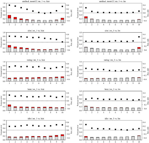
For all forecast approaches, some of the extreme portfolios yield the largest average forecast errors. In particular, the expected illiquidity of bonds with (1) a high and low historical illiquidity, (2) a large and small amount outstanding, (3) a high rating, (4) a low exposure to bond market (systematic) risk, and (5) high idiosyncratic risk are more difficult to predict. The graphs further suggest that neural networks reduce the forecast errors relative to the hist (lefthand column) and lm (righthand column) models for nearly all decile portfolios. This is indicated by percentage differences larger than zero (the squares above the dashed line), implying that the nn_1 model delivers more accurate illiquidity predictions. The figure further emphasizes that the higher average MSEs for the historical illiquidity–based approach and linear regressions (see Panel A of Table 5) obey more general patterns and are not driven by high forecast errors for only a few bonds with specific characteristics. Compared to the two benchmark models, the reduction in forecast errors when using neural networks are strongest for extreme decile portfolios (which are more difficult to predict), both in absolute and relative terms. Because this pattern is apparent for the comparison with both the historical illiquidity–based approach and linear regressions, we attribute the reduction in forecast errors to two effects: (1) the inclusion of slow-moving bond characteristics as predictors (in both the lm and the nn_1 model) and (2) the nn_1 model’s ability to capture nonlinearity and interactions.

Characteristics of Expected Illiquidity-Sorted Portfolios

In a next step, we examine whether statistically more accurate forecasts translate into economic gains in a portfolio formation exercise.¹⁷ In particular, we sort all bonds into decile portfolios based on expected illiquidity at the end of each month $t.$ Separately for each model and decile portfolio, we then calculate the equally weighted mean of future realized illiquidity. Panel A of Table 6 presents the time-series averages of monthly portfolio illiquidity (amihud measures). The last column adds results for the hypothetical case in which the sorting criterion is the bonds’ future realized illiquidity (real) rather than a forecast model’s estimates, thus mimicking perfect foresight. Panel B replicates the procedure outlined above for each model but selects weights that differ from the equal weights to calculate the average illiquidity within each decile portfolio. In particular, the optimizer aims to minimize the sum of squared deviations from the equal-weighting scheme, while requiring the portfolio-level rating (rating), yield (yield), and duration (dur) for the machine learning methods to be equal to those for the historical benchmark model. This framework ensures a straightforward comparison between machine learning–based methods and the historical illiquidity benchmark. It allows for more comparable decile portfolios and helps to avoid differences in expected illiquidity-sorted portfolios that are driven by differences in their exposure to rating, yield, and duration.

Table 6. Illiquidity of Decile Portfolio Sorts

	Forecast model						Reference
	hist	lm	elanet	rf	gbrt	nn_1	real
Panel A: Raw portfolio sorts
Low (L)	0.32	0.28	0.28	0.27	0.27	0.27	0.21
2	0.57	0.53	0.53	0.53	0.53	0.53	0.42
3	0.72	0.69	0.69	0.70	0.70	0.70	0.58
4	0.82	0.81	0.81	0.82	0.82	0.83	0.71
5	0.91	0.91	0.92	0.93	0.92	0.93	0.82
6	0.98	1.00	1.00	1.01	1.02	1.01	0.94
7	1.06	1.08	1.08	1.07	1.08	1.08	1.06
8	1.13	1.16	1.16	1.15	1.14	1.14	1.20
9	1.24	1.24	1.24	1.23	1.23	1.23	1.40
High (H)	1.44	1.46	1.47	1.47	1.47	1.46	1.83
H − L	1.12	1.18	1.19	1.20	1.20	1.19	1.62
t value	−	7.01	12.16	11.37	10.11	5.83	−
Panel B: Portfolio sorts with controls for rating, yield, and duration
Low (L)	0.32	0.29	0.28	0.28	0.28	0.28	0.21
2	0.57	0.53	0.53	0.52	0.52	0.52	0.42
3	0.72	0.70	0.70	0.69	0.69	0.68	0.58
4	0.82	0.82	0.82	0.83	0.82	0.81	0.71
5	0.91	0.92	0.93	0.94	0.93	0.91	0.82
6	0.98	1.01	1.01	1.01	1.01	1.00	0.94
7	1.06	1.08	1.08	1.07	1.07	1.08	1.06
8	1.13	1.15	1.15	1.14	1.14	1.15	1.20
9	1.24	1.24	1.24	1.26	1.26	1.28	1.40
High (H)	1.44	1.45	1.47	1.48	1.50	1.53	1.83
H − L	1.12	1.17	1.19	1.20	1.22	1.24	1.62
t value	−	3.69	7.29	6.72	10.18	10.63	−

Notes: This table examines differences in the predictive power of the different bond illiquidity forecast models (hist, lm, elanet, rf, gbrt, and nn_1) from an economic perspective. Bonds are first sorted into decile portfolios based on illiquidity predictions (the average monthly amihud measure) at the end of each month $t.$ The equally weighted mean of future realized illiquidity is calculated separately for each model and decile portfolio. Panel A presents the time-series averages of monthly figures. The last column adds the corresponding results for the hypothetical case in which the sorting criterion is the bonds’ future realized illiquidity, that is, assuming perfect foresight. Panel B replicates the procedure for each model but selects weights that slightly differ from the equal weights to calculate the average illiquidity within each decile portfolio. The optimizer aims to minimize the sum of squared deviations from the equal-weighting scheme, while requiring the portfolio-level rating (rating), yield (yield), and duration (dur) for the machine learning methods to be equal to those for the hist model. H − L denotes the spread between the estimates in the high- and low-illiquidity portfolios. A higher spread indicates that a given model is better at disentangling more liquid from less liquid bonds, which suggests economic value added for investors in the form of transaction cost savings. The t values (using Newey–West standard errors with 11 lags) are reported for the null hypothesis that the H − L illiquidity spread of a given column model (lm, elanet, rf, gbrt, or nn_1) is not different from the H − L spread of the historical illiquidity benchmark (hist). The baseline sample includes intraday transaction records for the US corporate bond market reported in the enhanced version of Trade Reporting and Compliance Engine (TRACE) for the sample period from July 2004 to November 2020.

The results in Table 6 highlight that differences in statistical predictive performance translate into differences in economic profitability. While the benchmark model and all machine learning models capture the cross-sectional variation in realized illiquidity, their ability to disentangle more liquid from less liquid bonds differs. Average realized illiquidity within the decile portfolios obtained from expected illiquidity line up monotonically with average realized illiquidity within the perfect-foresight decile portfolios, resulting in positive average H–L spreads that are statistically significant (not reported) and economically large. Again, focusing on a comparison between the historical illiquidity–based approach and the nn_1 model, we observe that for more liquid portfolios (e.g., decile 1), the average realized illiquidity for neural networks (0.27%) is lower and comes closer to the true value of 0.21% than that for the hist model (0.32%). For less liquid portfolios (e.g., decile 10), the average realized illiquidity for the nn_1 model (1.46%) is slightly higher and also closer to the true value of 1.83% than that for the historical illiquidity–based approach (1.44%). This results in a 7 basis points larger H–L spread (1.19% for nn_1 vs. 1.12% for hist). The differences between machine learning models and the benchmark model become more pronounced after controlling for the decile portfolios’ exposures to rating, yield, and duration (especially for less liquid portfolios), resulting in an almost 11% larger H–L spread (1.24% for nn_1 vs. 1.12% for hist).

Overall, machine learning techniques are better at disentangling more liquid from less liquid bonds than the historical illiquidity benchmark, which suggests economic value added to institutional investors.¹⁸ Due to the large transaction volumes in the corporate bond market, even the smallest improvements in illiquidity estimates will result in considerable transaction cost savings either directly in terms of a lower average bid–ask spread or indirectly in terms of a lower average price impact. Reduced transaction costs, in turn, have an immediate effect on improving a portfolio’s risk–return profile.

A Simple Example

To illustrate the importance of illiquidity predictions for the performance of fixed-income funds by way of an example that exploits the ranking performance of the different prediction models, take an average institutional investor with a bond portfolio size of $1 billion and a portfolio turnover of 5% per month. Moreover, assume that the average bond portfolio consists of 2,000 bonds and that the portfolio’s annualized alpha is 1.0%. Ignoring other transaction costs, without any price impact, this investor would be able to sell and buy bonds to rebalance their portfolio for $5\%\times \$1 \mathrm{\text{billion}}=\$50 \mathrm{\text{million}}$ of bonds traded each month ($\$600 \mathrm{\text{million}}$ of bonds traded per year). Assuming a 0.92% Amihud (2002) price impact (the average across deciles 1–10 in the right-most column labeled “Reference” in Panel B of Table 6) results in a $0.92\%\times 5\%=4.6 \mathrm{\text{bps}}$ reduction in monthly alpha or 0.55% in annual alpha, wiping out $5.5 million per year, that is, more than half of the average annual gain of $1\%\times \$1 \mathrm{\text{billion}}=\$10 \mathrm{\text{million}}$ (before any other transaction costs).

The Amihud (2002) illiquidity measure is highly variable across our bond universe, for example, the least liquid decile incurs a nearly nine times higher price impact than the most liquid one (1.83% vs. 0.21% in Table 6). Better illiquidity predictions help to control average turnover costs by enabling investors to focus on the most liquid decile portfolios (and sorting out the least liquid decile portfolios) when rebalancing their exposure. Assuming perfect foresight, avoiding the 50% least liquid part of the market hypothetically reduces the average price impact by a factor of 2.3 (0.55% for deciles 1–5 vs. 1.29% for deciles 6–10 based on the averages in the column labelled “Reference” in Panel B of Table 6), improving portfolio turnover costs by $0.92\%-0.55\%=0.37\%$ per year. By allocating trading to the most liquid bonds (and avoiding the least liquid ones), for example, by allocating a weight of 50% on the 10% most liquid bonds, 25% on the second-most liquid, and so on, the investor can even maintain her market impact costs below $50\%\times 0.21\%+25\%\times 0.42\%+12.5\%\times 0.58\%+6.25\%\times 0.71\%+6.25\%\times 0.82\%=0.38\%$ per year. Estimating the costs associated with specific securities is crucial for generating excess returns in classification strategies. Machine learning models are effective in this regard, surpassing the historical illiquidity–based prediction model and reducing expected market impact by 12.5% (0.28% for the nn_1 model vs. 0.32% for the hist model) for the 10% and about 4% (0.64% for the nn_1 model vs. 0.67% for the hist model using the allocation weights) for the 50% most liquid bonds.

Finally, assume that the hypothetical investor wants to avoid the 50% least liquid bonds and concentrates portfolio turnover on the most liquid bonds as outlined above, but does not observe the real illiquidity distribution before trading. Relying on the historical illiquidity–based model would translate into 0.50% annual cost (i.e., the average of deciles 1–5 in the column labeled “hist” in Table 6, Panel B). Therefore, the cost of being unable to observe the future realized market impact ex ante is a 32% increase of the market impact compared to the hypothetical perfect foresight scenario of 0.38% (see above). The machine learning–based models can mitigate this cost by providing more accurate estimates of future illiquidity. For example, the nn_1 model only leads to an increase of 21% (0.46%) relative to the perfect-foresight case (0.38%), that is, an 11 pps (32%−21%) reduction compared to the benchmark based on historical illiquidity (0.50%).

Cross-Sectional Bond Returns

A natural extension of our analysis is to measure cross-sectional bond returns. In particular, we again sort bonds into decile portfolios based on their historical illiquidity or expected illiquidity at the end of each month t (using the hist, lm, and nn_1 models). We then compute the portfolio return in the next month t + 1. The results for the full sample and three subperiods are shown in Table 7. As expected, bonds in decile 10 (more illiquid bonds) outperform bonds in decile 1 (less illiquid bonds). Even more important from an asset pricing perspective, the H − L spread is higher for the machine learning–based prediction models (lm and nn_1) compared to the historical illiquidity model (hist). The same results continue to hold for bond returns over the next 12 months (not reported). Prediction models using machine learning techniques generate a higher illiquidity premium in the cross-section of bond returns than the benchmark model. These results support Amihud and Mendelson’s (1986) insight that investors require higher returns for more illiquid bonds to compensate them for their higher trading expenses.

Table 7. Returns of Decile Portfolio Sorts

	2012–2020			2012–2014			2015–2017			2018–2020
	hist	lm	nn_1	hist	lm	nn_1	hist	lm	nn_1	hist	lm	nn_1
Low (L)	0.38	0.37	0.36	0.55	0.53	0.48	0.27	0.29	0.30	0.34	0.32	0.31
2	0.38	0.38	0.39	0.50	0.54	0.55	0.29	0.30	0.31	0.36	0.34	0.32
3	0.40	0.38	0.40	0.53	0.50	0.52	0.32	0.31	0.35	0.36	0.33	0.36
4	0.41	0.40	0.40	0.51	0.47	0.48	0.36	0.38	0.37	0.38	0.35	0.36
5	0.45	0.40	0.42	0.53	0.50	0.52	0.47	0.37	0.39	0.37	0.35	0.35
6	0.46	0.44	0.42	0.51	0.54	0.51	0.48	0.44	0.39	0.40	0.35	0.39
7	0.43	0.46	0.47	0.50	0.50	0.52	0.42	0.48	0.46	0.39	0.41	0.44
8	0.49	0.48	0.47	0.52	0.51	0.47	0.52	0.50	0.48	0.42	0.43	0.44
9	0.49	0.53	0.51	0.54	0.57	0.56	0.53	0.54	0.53	0.41	0.48	0.44
High (H)	0.58	0.65	0.64	0.65	0.71	0.72	0.64	0.70	0.73	0.46	0.53	0.49
H − L	0.20	0.27	0.29	0.10	0.19	0.25	0.37	0.41	0.43	0.12	0.21	0.18

Notes: This table presents differences in the predictive power of the different bond illiquidity forecast models (hist, lm, and nn_1) for cross-sectional bond returns. Bonds are first sorted into decile portfolios based on their historical illiquidity or expected illiquidity (using the average monthly amihud measure) at the end of each month $t.$ In a second step, the equally weighted return is calculated for each prediction model and decile portfolio in the next month $t+1$ (in % per month). H − L denotes the spread between the estimates in the high- and low-illiquidity portfolios. A higher spread indicates that a given model generates a higher illiquidity premium in the cross-section of bond returns. Returns are reported for the full test sample and three subperiods (2011–2013, 2014–2016, 2017–2019). The baseline sample includes intraday transaction records for the US corporate bond market reported in the enhanced version of Trade Reporting and Compliance Engine (TRACE) for the sample period from July 2004 to November 2020.

Practical Implications

Comparing our findings for the statistical assessment with the economic performance of our different forecast methods reveals another issue that seems particularly important from a practitioner’s perspective. While the results in Tables 4 and 5 suggest that nonlinear machine learning models (rf, gbrt, and nn_1) strongly outperform both the historical benchmark (hist) and their linear counterparts (lm and elanet) when it comes to level predictions of illiquidity, as measured by a statistical comparison of their forecast errors, the results are more nuanced for the mere rank forecasts. In general, machine learning methods perform better than the historical illiquidity benchmark in sorting bonds into expected illiquidity portfolios, but the difference becomes less pronounced when comparing linear and nonlinear machine learning models with each other. For example, in Panel A of Table 6, the difference in the H–L spreads between the lm (1.18) and nn_1 (1.19) methods is negligible, but it becomes larger when appropriately controlling for risk in Panel B (1.17 for lm vs. 1.24 for nn_1). In Table 7, the lm model even generates a slightly higher illiquidity premium than the nn_1 model during the last subperiod (2018–2020). In all other subperiods, the nn_1 model dominates the lm model marginally. These patterns are important for the practical implementation in portfolio management because neural networks in particular are computationally extremely costly.

In light of these findings, whether the complexity and resourcefulness of more sophisticated machine learning methods is justified in the asset management practice most likely depends on the specific application. If illiquidity predictions are merely used to rank bonds and sort out the least liquid ones, as illustrated in the example above, models that incorporate a set of predictor variables (in addition to historical illiquidity) in a linear way seem satisfactory and are straightforward to implement. However, in contrast to such relatively simple ranking and/or sorting exercises, there are many use cases that require the highest possible accuracy of illiquidity level predictions. In particular, practical applications that involve bond portfolio optimization under the constraint to minimize transaction costs should benefit from more complex machine learning methods that account for nonlinearity and multiway interactions. Furthermore, the benefits from nonlinear models may be more important at some times than at others. For example, Drobetz et al. (2024) show that more complex models are required during turbulent times when predictions become more difficult.

To provide a specific example, we note that accurate forecasts of corporate bond illiquidity are highly important from a regulatory perspective. The “SEC Liquidity Rule” requires that 85% of a fund could be liquidated in fewer than five days with a maximum participation of 20% of daily dollar trading volumes to be applied to a corporate bond portfolio. If the fund mimics the performance of a corporate bond index, as most exchange-traded funds attempt to do, the portfolio construction process should be viewed as a tracking error minimization under some liquidity and capacity constraints. While capacity constraints may be based on estimates of the bonds’ trading volumes, controlling for turnover costs depends more on price impact measures, such as the Amihud (2002) illiquidity measure. Corporate bond ETFs are known to achieve lower Sharpe ratios because such instruments must pay for liquidity (Houweling 2011). As a result, the ability to accurately forecast bond illiquidity is crucial for improving capacity and turnover costs of such replicating strategies and, based on our statistical analysis of level forecast errors, more complex machine learning–based models seem to be most appropriate to accomplish this task. More generally, this argument is true for any mutual bond fund that has achieved a certain size. Because regulatory liquidity requirements must be met at all times, this can prove to be difficult as funds become large, unless they are willing to pay or make their investors pay for liquidity.

Characteristics and Functioning Scheme of Machine Learning Estimators

Recognizing that machine learning–based models outperform the historical illiquidity benchmark and that nonlinearity as well as interactions can further help in accurately modeling expected bond illiquidity, we now focus on determining how these techniques, which are often referred to as “black boxes,” achieve outperformance. This black box problem is addressed by examining the characteristics and functioning scheme of neural networks, focusing particularly on the nn_1 model.¹⁹ We decompose predictions into the contributions of individual variables using relative variable importance metrics and explore patterns of nonlinear and interactive effects in the relationship between predictor variables and illiquidity estimates.

Variable Importance

We begin with investigating which variables are, on average, most important for the predictions obtained from linear regressions (lm) and neural networks (nn_1). Given that we re-estimate our models on an annual basis, it is also instructive to inspect whether a predictor’s contribution to the overall forecast ability of a model changes over time. Separately for each model and re-estimation date, we compute the variable importance matrix using a two-step approach: First, we compute the absolute variable importance as the increase in MSE from randomly permuting the values of a given predictor variable in the training sample. Second, we normalize the absolute variable importance measures to sum to one, signaling the relative contribution of each variable to the lm and nn_1 model.

Analyzing the relative variable importance metrics over time, more volatile metrics indicate that all covariates in the predictor set should be considered important. In contrast, stable metrics mean we should remove uninformative predictors permanently, as they may decrease a model’s signal-to-noise ratio. Figure 2 depicts the relative variable importance metrics over the sample period for linear regressions (Panel A) and neural networks (Panel B). To allow for better visual assessment, we omit the bars for the historical illiquidity predictor. The relative variable importance of amihud_hist can be inferred by subtracting the aggregate relative importance of all other predictors from one. On average, both models place the largest weight on historical illiquidity; this predictor accounts for more than 40% of the aggregate average variable importance for the lm model but only around 35% for the nn_1 model. On the one hand, high weights are expected because realized illiquidity is persistent and has long-memory properties. On the other hand, the lower weight placed on historical illiquidity by neural networks relative to linear regressions helps to explain why the nn_1 model outperforms the lm model in terms of lower forecast errors in general, but especially within extreme decile portfolios sorted on historical illiquidity (see Figure 1). Linear regressions miss out on extracting valuable information from the nonlinear and interactive patterns in the relationship between our set of fundamental as well as macroeconomic predictor variables and expected illiquidity.

Figure 2. Variable Importance

Notes: This figure shows the relative importance of the variables included as predictors in linear regressions (Panel A) and neural networks (Panel B) at each re-estimation date. For this purpose, the relative variable importance matrix is calculated based on a two-step approach: First, the absolute variable importance is computed as the reduction in R² from setting all values of a given predictor to zero within the training sample. Second, the absolute variable importance measures are normalized to sum to 1, signaling the relative contribution of each variable to a model. The baseline sample includes intraday transaction records for the US corporate bond market reported in the enhanced version of Trade Reporting and Compliance Engine (TRACE) for the sample period from July 2004 to November 2020.

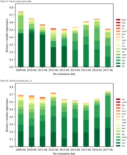
Among the remaining variables, the two models identify slightly different predictors as most relevant for estimating illiquidity. While the lm model considers the default spread (dfy) highly informative, neural networks predominantly extract information from fundamental predictors. In particular, the bond-level predictor duration (dur), size (size), and maturity (mat) are most important for the nn_1 model, accounting for roughly 18%, 18%, and 14% of the aggregate average variable importance, respectively. In contrast, the default spread (dfy) is much less informative for neural network models. Accordingly, given the superior predictive performance of the nn_1 model, the time variation in bond illiquidity is driven more by changes in bond characteristics than by changes in the underlying economic conditions. Moreover, while most variables have some relevance based on their average metrics, the analysis reveals that these metrics change notably over time. Because this time variation is apparent for all predictor variables, we conclude that each variable is an important contributor in all models, albeit to varying degrees. Overall, the variable importance results in Figure 2 do not recommend that we should remove specific predictors.²⁰

Nonlinearity and Interactions

Tree-based models and neural networks are superior to the historical illiquidity benchmark, and they also tend to outperform linear regressions with the same set of covariates. A large part of this outperformance must be attributable to their ability to exploit nonlinear and interactive patterns in the relationship between predictors and expected bond illiquidity. Therefore, in a final step, we analyze in more detail whether and how neural networks (nn_1) capture nonlinearity and interactions. For comparison, we contrast the results with illiquidity estimates obtained from linear regressions (lm).²¹

We first examine the marginal association between a single predictor variable and its illiquidity predictions ($I_{i,t+k|t}^F,$ with $k=12$). As an example, we select a bond’s duration (dur), one of the most influential predictors in our analysis (see Figure 2). To visualize the average effect of dur on $I_{i,t+k|t}^F,$ we set all predictors to their uninformative median values within the training sample at each re-estimation date. We then vary dur across the minimum and maximum values of its historical distribution and compute the expected illiquidity. Finally, we average the illiquidity predictions across all re-estimation dates.

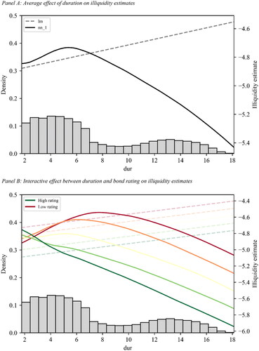
Panel A of Figure 3 illustrates the marginal association between dur and $I_{i,t+k|t}^F$ for linear regressions (dashed line) and neural networks (solid line), respectively. We add a histogram that depicts the historical distribution of dur. This visualization allows us to assess the empirical relevance of differences in predictions obtained from the lm and nn_1 models for the overall forecast results. At the left end of the distribution, approximately within the ($+1.8,+6.3$) interval, the predictions obtained from linear regressions and neural networks are similar. We identify an increasing linear relationship between dur and $I_{i,t+k|t}^F$ for the lm model and a close-to-linear relationship for the nn_1 model, suggesting that bonds with a shorter duration are more liquid than their medium-duration counterparts. However, outside this interval, the marginal association between duration and expected illiquidity delineated in the neural network model is strongly negative, suggesting that bonds with a longer duration are also likely to be more liquid than their medium-duration counterparts. Overall, this leads to a nonsymmetrical inverted U-shaped relationship for the nn_1 model. In sharp contrast, the lm model, by construction, must continue to follow the increasing linear relationship over the entire range of duration, resulting in illiquidity estimates from linear regressions that diverge substantially from those obtained using neural networks.

Figure 3. Nonlinear and Interactive Effects in Estimating Corporate Bond Illiquidity

Notes: This figure examines the models’ ability to capture nonlinear and interactive effects in estimating future bond illiquidity (the average monthly amihud measure). Panel A illustrates the marginal association between bond duration (dur) and its illiquidity estimates ($I_{i,t+k|t}^F,$ with $k=12$) for linear regressions (dashed line) and neural networks (solid line), respectively. It also shows a histogram that depicts the historical distribution of dur. To visualize the average effect of dur on $I_{i,t+k|t}^F,$ all predictors are set to their uninformative median values within the training sample at each re-estimation date. In the next step, dur is varied over the minimum and maximum values of its historical distribution, and the illiquidity estimates are computed. Finally, the average illiquidity estimates across all re-estimation dates are estimated and presented in the panel. Panel B shows the interactive effect between dur and bond rating (rating) on $I_{i,t+k|t}^F.$ To this end, the procedure outlined above is replicated, but this time the illiquidity estimates are computed for different levels of rating across its minimum and maximum values. Low and high levels for rating are marked with red and green lines; dashed and solid lines refer to linear regressions (lm) and neural networks (nn_1), respectively. The baseline sample includes intraday transaction records for the US corporate bond market reported in the enhanced version of Trade Reporting and Compliance Engine (TRACE) for the sample period from July 2004 to November 2020.

The nonsymmetrical inverted U-shaped relationship between dur and $I_{i,t+k|t}^F$ (compared to an increasing linear relationship) is more consistent with (1) the empirical patterns observed when plotting duration and realized illiquidity during the out-of-sample period simultaneously (not reported) and (2) anecdotal evidence. Anecdotal evidence is twofold. First, the number of institutional investors with a natural duration target (e.g., property and casualty vs. life insurance companies) is higher for both ends of the yield curve because they attempt to match their short-term and long-term liabilities, respectively. Therefore, these types of bonds, that is, with either a lower or a higher duration, are issued more frequently (consistent with the historical distribution of dur depicted by the histogram). Importantly, they are also traded more frequently, thereby increasing their liquidity. Second, institutional investors are likely to increase (decrease) their portfolio’s duration by buying high-duration (low-duration) bonds when they expect interest rates to rise (fall). This behavior is another reason for lower- and higher-duration bonds to be traded more frequently, increasing their liquidity further. Because a considerable share of our observations lies within the lower and upper parts of the historical distribution, the differences in predictions are practically relevant. Our analysis highlights the need to allow for nonlinear impacts of the predictor variables on expected illiquidity. We further note that nonlinear relationships (both U- and S-shaped) are similarly observable for other predictors (not reported), for example, a bond’s historical illiquidity (amihud_hist), maturity (mat), size (size), and age (age).

Next, we investigate between-predictor interactions in estimating corporate bond illiquidity, referring again to dur as our baseline covariate. In addition, we select rating, another highly influential predictor (see Figure 2), as our interactive counterpart and replicate the procedure just described. In this case, we compute expected illiquidity for different levels of rating across its minimum and maximum values. The interactive effect between dur and rating on $I_{i,t+k|t}^F$ is illustrated in Panel B of Figure 3. Low and high levels for rating are marked as red and green lines, respectively. If there is no interaction, or if the model is unable to capture interactions, computing expected illiquidity for different levels of rating shifts the lines from Panel A up- or downward in parallel. In this case, the distance between the lines is identical for any given value of dur. This pattern is apparent for linear regressions (drawn as dotted lines), because no prespecified interaction term, for example, dur $\times$ rating for the interaction between dur and rating, is included as a predictor in the linear regression framework. The dotted lines are shifted downward when rating increases, indicating that an increase in rating that is independent of the bond’s duration decreases $I_{i,t+k|t}^F.$

For neural networks, the same pattern is only observable for the right end of the dur distribution. In contrast, at the left end of the distribution, unlike the lm model, the nn_1 model uncovers interactive effects between dur and a bond’s rating in predicting illiquidity.²² This interactive effect is so strong that it reverses the isolated effects of duration and rating on expected illiquidity, that is, bonds with a shorter duration and, at the same time, a higher rating tend to be less liquid than their lower-rating counterparts. This finding is again consistent with anecdotal evidence. Liquidity of high-yield bonds is concentrated at the short-term part of the curve because these bonds tend to have shorter durations. On average, however, bond liquidity decreases with higher credit risk. The reverse is true for the shorter-term part of the curve, which one could perceive as counterintuitive. An explanation is that our machine learning models have been fitted predominantly during a sample period with historically low interest rates. In this “zero lower bound” environment, many institutional investors adapted to yield scarcity by taking on more risk, that is, they shifted their focus to lower-rated bonds to meet their need for income. With respect to duration, they often chose shorter-duration bonds with lower ratings, for example, high-yield bonds, as opposed to their higher-rating counterparts. This change in preferences has led to a relative shift in demand, which may have contributed to a decrease in the liquidity of bonds with a higher rating.

Taken together, these visualizations provide an explanation for our main finding that more complex machine learning models, such as regression trees and neural networks, are able to generate more accurate bond illiquidity forecasts than their linear counterparts. Linear regressions (both simple and penalized), by construction, cannot capture nonlinear and multiway interactive effects that seem to describe real-world phenomena in a much better way. In this light, our analysis helps to explain the outperformance of regression trees and neural networks (which “learn” these complex patterns from the training and validation data) over the historical illiquidity benchmark and linear regression models in terms of lower forecast errors.

Conclusion

Understanding a bond’s multi-faceted liquidity characteristics and predicting bond illiquidity are relevant topics from an asset pricing point of view, but they are equally important from a regulatory and real-word investor perspective. Our paper contributes to a better understanding of the characteristics of corporate bond illiquidity and of how to transform this information into reliable illiquidity forecasts. In particular, we compare the predictive performance of machine learning–based illiquidity estimators (linear regressions, tree-based models, and neural networks) to that of the historical illiquidity benchmark, which is the most commonly used model. All machine learning models outperform the historical illiquidity–based approach from both a statistical and an economic perspective. The outperformance is attributable to these models’ ability to exploit information from a large set of bond characteristics that impact bond illiquidity. Tree-based models (random forests and gradient-boosted regression trees) and neural networks perform similarly and work remarkably well. These more complex approaches outperform linear regressions with the same set of covariates, particularly in terms of prediction level accuracy, because of their ability to utilize nonlinear and interactive patterns. From a practitioner’s perspective, our results suggest that the choice of the appropriate machine learning model depends on the specific application, such as simple bond rankings and sortings based on expected illiquidity as opposed to bond portfolio optimizations that require level forecasts of illiquidity. An obvious open question is whether our findings can be transferred to corporate bonds for which historical illiquidity data are not readily available. We leave this task for future research.

Acknowledgments

The authors thank Daniel Giamouridis (the journal's associate editor), two anonymous referees, Yakov Amihud, Maxime Bucher, Tristan Froidure, Patrick Houweling, Harald Lohre, Robert Korajczyk, Daniel Seiler, Michael Weber, and the participants of the Mannheim Finance faculty seminar for insightful suggestions and remarks.

Disclosure statement

No potential conflict of interest was reported by the author(s).

Additional information

Notes on contributors

Axel Cabrol

Axel Cabrol, CFA, is Co-Deputy CIO at TOBAM, Paris, France.

Wolfgang Drobetz

Wolfgang Drobetz is a Professor of Finance at the Faculty of Business Administration, University of Hamburg, Hamburg, Germany.

Tizian Otto

Tizian Otto is a Postdoctoral Researcher in Finance at the Faculty of Business Administration, University of Hamburg, Hamburg, Germany.

Tatjana Puhan

Tatjana Puhan is Head of Asset Allocation at Swiss Re Management Ltd, Zurich, Switzerland and Adjunct Faculty Member at the Faculty of Business Administration, University of Mannheim, Mannheim, Germany.

Notes

1 Other papers in this research area that find evidence for superior stock selection based on a large set of predictors are Rasekhschaffe and Jones (2019), Chen, Pelger, and Zhou (2022), and Bryzgalova, Pelger, and Zhou (2023). Related studies document similar results for international data (Tobek and Hronec 2021), European data (Drobetz and Otto 2021), emerging markets data (Hanauer and Kalsbach 2023), Chinese data (Leippold et al., 2023), and crash prediction models (Dichtl, Drobetz, and Otto 2023).

2 Reichenbacher, Schuster, and Uhrig-Homburg (2020) also use a large set of predictors for expected bond liquidity, but they work with the linearity assumption in their estimation model.

3 We use the enhanced version of TRACE instead of the standard version because it additionally contains uncapped transaction volumes and information on whether the trade is a buy, a sell, or an interdealer transaction. This refinement enables us to construct measures that capture different aspects of bond illiquidity based on intraday bond transactions.

4 The detailed transaction data allow us to compute direct liquidity measures as opposed to indirect measures based on bond characteristics and/or end-of-day prices (Houweling, Mentink, and Vorst 2005).

5 To control for return outliers not driven by illiquidity, we omit observations with daily amihud measures exceeding 5% on a given day. Our main results remain qualitatively similar when using other cut-off thresholds, e.g., 1% or 10%.

6 Because no prior study has examined whether this set of variables is helpful for predicting bond illiquidity, a potential lookahead bias should not be an issue in our analysis.

7 Alternatively, one-month and five-year forecast horizons are common in the literature ($k=1$ and $k=60,$ respectively). Both alternatives have shortcomings in our setup, which is why we opt for a one-year forecast horizon. First, one-month illiquidity measures are very noisy, which hampers the evaluation of forecast errors. Second, forecast horizons much longer than 12 months are less common in the industry due to the underlying nature of fiscal years.

8 Because we apply on a one-year forecast horizon, there is a one-year gap between the end of the sample that is used for training and validation (2010:06) and the estimation date (2011:06).

9 Neural network models are computationally intensive and can be specified in innumerable different architectures. We retreat from tuning parameters (e.g., the size of batches or the number of epochs) and specify five different models, assuming that our nn_1-nn_5 architectures are a conservative lower bound for the predictive performance of neural network models. Because the predictive performance of neural network models deteriorates slightly in the number of hidden layers in our application (not reported), we only present the results for the nn_1 architecture.

10 Following Becker et al. (2021), we omit bonds with fewer than 50 illiquidity estimates to allow for valid inference.

11 The cross-sectional and time-series means for realized illiquidity are −4.75 and −4.78, respectively (not reported).

12 In most economic applications, when comparing different models, a single model does not exist that significantly dominates all competitors because the data are not sufficiently informative to provide an unequivocal answer. However, it is possible to reduce the set of models to a smaller set of models—the so-called model confidence set (MCS)—that contains the best model(s) with a given level of confidence. Hansen, Lunde, and Nason’s (2011) MCS determines the set of models that composes the best model(s) from a collection of models, where “best” is defined in terms of the MSE. Informative data will result in a MCS that contains only the best model. Less informative data make it difficult to distinguish between models and result in a MCS that contains several models. In our applications, we examine statistical significance at the 5% level, translating into 95% model confidence sets.

13 According to Gu, Kelly, and Xiu (2020), DM test statistics are asymptotically $N\left(0,1\right)$-distributed and test the null hypothesis that the divergence between two models is zero. They map to p-values in the same way as regression t-statistics.

14 Due to limited data availability, the test sample in our baseline setting does not contain the 2007–2008 global financial crisis, during which the availability of credit suddenly plummeted. In a robustness test (not reported), we shorten the length of the sample used for training and validation to three years in order to include the global financial crisis in the test sample. Again, all machine learning models dominate the historical illiquidity–based model during this severe crisis.

15 Table C2 in Online Supplemental Appendix C confirms that this conclusion remains robust for our two other illiquidity measures: t_volume and t_spread. To check robustness even further, this table also contains the results for two additional illiquidity measures: First, we apply Lesmond, Ogden, and Trzcinka’s (1999) illiquidity measure based on zero daily bond returns (p_zeros), where a larger fraction of zero returns in a given sample month indicates lower liquidity. Second, we use Roll’s (1984) implicit measure of the bid–ask spread based on the covariance of daily bond returns and their lagged returns (Roll’s spread). To this end, we calculate the negative autocorrelation of bond returns within a given sample month, with higher numbers indicating lower liquidity. The results are qualitatively similar, albeit the performance advantage of machine learning models is less pronounced for the p_zeros measure.

16 In a robustness test, we implement a Giacomini–White (2006) test for conditional predictive performance. The DM test is unconditional in the sense that it asks which forecast was more accurate, on average, in the past; it may thus be appropriate for making recommendations about which forecast may be better for an unspecified future date. As elaborated in Giacomini and White (2006), “the conditional approach asks instead whether we can use available information—above and beyond past average behavior—to predict which forecast will be more accurate for a specific future date” (p. 1547). To describe the specific future date, we use the default spread at the end of the last month as the conditioning variable that captures the prevailing state of the economy. The results are presented in Table C3 in Online Supplemental Appendix C. All test statistics indicate statistical significance. Overall, the results support the DM tests. Machine learning–based forecast methods outperform the historical illiquidity benchmark not only in terms of their unconditional predictive ability but also in terms of their conditional predictive ability.

17 Online Supplemental Appendix B presents an alternative test for classification performance based on confusion matrices that contrasts predicted and realized classes, together with accuracy and ranking loss as classification measures. Machine learning–based methods produce a superior misclassification distribution, which may translate into economic outperformance.

18 Table 6 also contains the t-statistics (using Newey-West standard errors with 11 lags) for the null hypothesis that the H–L illiquidity spread of a given column model (lm, elanet, rf, gbrt, or nn_1) is not different from the H–L spread of the historical illiquidity-based model (hist). All t-statistics for pairwise differences in portfolio means indicate statistical significance, i.e., the null hypothesis of indifference can be rejected in all cases, thus confirming that machine learning techniques are reliably better at disentangling more liquid from less liquid bonds.

19 Similar to random forests and gradient-boosted regression trees, neural networks exhibit low forecast errors (both on average and over time; see Table 5), produce accurate forecasts for bonds with extreme characteristics (see Figure 1), and perform well in a portfolio formation exercise (see Table 6).

20 To be on the conservative side, we compare the statistical and economic predictive performance of the original nn_1 model with versions that only consider the top 5 or 10 predictors in terms of their relative variable importance. Out-of-sample test results (not reported) suggest that no model version exhibits superior outperformance in any of these tests, so we choose not to remove unconditionally less informative variables from the predictor set and instead consider each predictor as informative (albeit to varying degrees). Furthermore, we caution that the pre-estimation variable selection based on relative importance metrics derived from the entire sample period could lead to foresight bias, undermining the credibility of out-of-sample tests.

21 The patterns and their implications are qualitatively similar when comparing gradient-boosted regression trees (gbrt) and neural networks (nn_1) to estimates obtained from penalized linear regressions (elanet). This result confirms that the ability to exploit nonlinear and interactive patterns leads to the outperformance of tree-based models and neural networks over linear regressions.

22 Despite being slightly less pronounced, the nn_1 model also reveals interactive effects between other bond characteristics in estimating future illiquidity, for example, between a bond’s historical illiquidity (amihud_hist) and size (size).

References

- Amihud, Y. 2002. “Illiquidity and Stock Returns: Cross-Section and Time-Series Effects.” Journal of Financial Markets 5 (1): 31–56. doi:10.1016/S1386-4181(01)00024-6.
- Amihud, Y., and H. Mendelson. 1986. “Asset Pricing and the Bid-Ask Spread.” Journal of Financial Economics 17 (2): 223–249. doi:10.1016/0304-405X(86)90065-6.
- Avramov, D., S. Cheng, and L. Metzker. 2022. “Machine Learning versus Economic Restrictions: Evidence from Stock Return Predictability.” Management Science 69 (5): 2587–2619. doi:10.1287/mnsc.2022.4449.
- Bali, T. G., A. Goyal, D. Huang, F. Jiang, and Q. Wen. 2020. Predicting Corporate Bond Returns: Merton Meets Machine Learning. Georgetown McDonough School of Business Research Paper No. 3686164.
- Bali, T. G., A. Goyal, D. Huang, F. Jiang, and Q. Wen. 2022. The Cross-Sectional Pricing of Corporate Bonds Using Big Data and Machine Learning, Working Paper.
- Bali, T. G., A. Subrahmanyam, and Q. Wen. 2021. “Long-Term Reversals in the Corporate Bond Market.” Journal of Financial Economics 139 (2): 656–677. doi:10.1016/j.jfineco.2020.08.007.
- Bao, J., J. Pan, and J. Wang. 2011. “The Illiquidity of Corporate Bonds.” The Journal of Finance 66 (3): 911–946. doi:10.1111/j.1540-6261.2011.01655.x.
- Becker, J., F. Hollstein, M. Prokopczuk, and P. Sibbertsen. 2021. “The Memory of Beta.” Journal of Banking & Finance 124 (1): 106026. doi:10.1016/j.jbankfin.2020.106026.
- Bessembinder, H., K. M. Kahle, W. F. Maxwell, and D. Xu. 2009. “Measuring Abnormal Bond Performance.” Review of Financial Studies 22 (10): 4219–4258. doi:10.1093/rfs/hhn105.
- Bessembinder, H., W. Maxwell, and K. Venkataraman. 2006. “Market Transparency, Liquidity Externalities, and Institutional Trading Costs in Corporate Bonds.” Journal of Financial Economics 82 (2): 251–288. doi:10.1016/j.jfineco.2005.10.002.
- Bianchi, D., M. Büchner, and A. Tamoni. 2021. “Bond Risk Premiums with Machine Learning.” The Review of Financial Studies 34 (2): 1046–1089. doi:10.1093/rfs/hhaa062.
- Blitz, D., T. Hoogteijling, H. Lohre, and P. Messow. 2023. “How Can Machine Learning Advance Quantitative Asset Management.” Journal of Portfolio Management 49 (9): 78–95.
- Bongaerts, D., F. de Jong, and J. Driessen. 2017. “An Asset Pricing Approach to Liquidity Effects in Corporate Bond Markets.” The Review of Financial Studies 30 (4): 1229–1269. doi:10.1093/rfs/hhx005.
- Bryzgalova, S., M. Pelger, and J. Zhu. 2023. “Forest through the Trees: Building Cross-Sections of Stock Returns.” Journal of Finance. Forthcoming.
- Chakravarty, S., and A. Sarkar. 2003. “Trading Costs in Three U.S. Bond Markets.” The Journal of Fixed Income 13 (1): 39–48. doi:10.3905/jfi.2003.319345.
- Chen, L., M. Pelger, and J. Zhou. 2022. “Deep Learning in Asset Pricing.” Management Science. Forthcoming.
- Cherief, A., M. Ben Slimane, J.-M. Dumas, and H. Fredj. 2022. “Credit Factor Investing with Machine Learning Techniques.” Working paper 128-2022, Amundi Asset Management.
- Chordia, T., A. Sarkar, and A. Subrahmanyam. 2005. “An Empirical Analysis of Stock and Bond Market Liquidity.” The Review of Financial Studies 18 (1): 85–129. http://www.jstor.org/stable/3598068.
- Cosemans, M., R. Frehen, P. C. Schotman, and R. Bauer. 2016. “Estimating Market Betas Using Prior Information Based on Firm Fundamentals.” Review of Financial Studies 29 (4): 1072–1112. doi:10.1093/rfs/hhv131.
- Dichtl, H., W. Drobetz, and T. Otto. 2023. “Forecasting Stock Market Crashes via Machine Learning.” Journal of Financial Stability 65: 101099. doi:10.1016/j.jfs.2022.101099.
- Dickerson, A., P. Mueller, and C. Robotti. 2023. “Priced Risk in Corporate Bonds.” Journal of Financial Economics 150 (2): 103707. doi:10.1016/j.jfineco.2023.103707.
- Dick-Nielsen, J. 2009. “Liquidity Biases in TRACE.” The Journal of Fixed Income 19 (2): 43–55. doi:10.3905/jfi.2009.19.2.043.
- Dick-Nielsen, J. 2014. How to Clean Enhanced TRACE Data, Working Paper.
- Dick-Nielsen, J., P. Feldhütter, and D. Lando. 2012. “Corporate Bond Liquidity before and after the on-Set of the Subprime Crisis.” Journal of Financial Economics 103 (3): 471–492. doi:10.1016/j.jfineco.2011.10.009.
- Diebold, F., and R. Mariano. 1995. “Comparing Predictive Accuracy.” Journal of Business & Economic Statistics 13 (3): 253–263. doi:10.1080/07350015.1995.10524599.
- Drobetz, W., F. Hollstein, T. Otto, and M. Prokopczuk. 2024. “Estimating Stock Market Betas via Machine Learning.” Journal of Financial and Quantitative Analysis 1–56. doi:10.1017/S0022109024000036.
- Drobetz, W., and T. Otto. 2021. “Empirical Asset Pricing via Machine Learning: Evidece from the European Stock Market.” Journal of Asset Management 22 (7): 507–538. doi:10.1057/s41260-021-00237-x.
- Fedenia, M., S. Nam, and T. Ronen. 2021. Machine Learning in the Corporate Bond Market and Beyond: A New Classifier, SSRN Working Paper.
- Freyberger, J., A. Neuhierl, and M. Weber. 2020. “Dissecting Characteristics Nonparametrically.” The Review of Financial Studies 33 (5): 2326–2377. doi:10.1093/rfs/hhz123.
- Friewald, N., R. Jankowitsch, and M. Subrahmanyam. 2012. “Illiquidity or Credit Deterioration: A Study of Liquidity in the US Corporate Bond Market during Financial Crises.” Journal of Financial Economics 105 (1): 18–36. doi:10.1016/j.jfineco.2012.02.001.
- Giacomini, R., and H. White. 2006. “Tests of Conditional Predictive Ability.” Econometrica 74 (6): 1545–1578. doi:10.1111/j.1468-0262.2006.00718.x.
- Gu, S., B. Kelly, and D. Xiu. 2020. “Empirical Asset Pricing via Machine Learning.” The Review of Financial Studies 33 (5): 2223–2273. doi:10.1093/rfs/hhaa009.
- Hanauer, M., and T. Kalsbach. 2023. “Machine Learning and the Cross-Section of Emerging Market Stock Returns.” Emerging Markets Review 55: 101022. doi:10.1016/j.ememar.2023.101022.
- Hansen, P. R., A. Lunde, and J. M. Nason. 2011. “The Model Confidence Set.” Econometrica 79 (2): 453–97.
- Hong, G., and A. Warga. 2000. “An Empirical Study of Bond Market Transactions.” Financial Analysts Journal 56 (2): 32–46. doi:10.2469/faj.v56.n2.2342.
- Hotchkiss, E., and G. Jostova. 2017. “Determinants of Corporate Bond Trading: A Comprehensive Analysis.” Quarterly Journal of Finance 07 (02): 1750003. doi:10.1142/S2010139217500033.
- Houweling, P. 2011. “On the Performance of Fixed Income Exchange Traded Funds.” The Journal of Index Investing 3 (1): 39–44. doi:10.3905/jii.2012.3.1.039.
- Houweling, P., A. Mentink, and T. Vorst. 2005. “Comparing Possible Proxies of Corporate Bond Liquidity.” Journal of Banking & Finance 29 (6): 1331–1358. doi:10.1016/j.jbankfin.2004.04.007.
- Jankowitsch, R., A. Nashikkar, and M. Subrahmanyam. 2011. “Priced Dispersion in OTC Markets: A New Measure of Liquidity.” Journal of Banking & Finance 35 (2): 343–357. doi:10.1016/j.jbankfin.2010.08.016.
- Kaufmann, H., P. Messow, and J. Vogt. 2021. “Boosting the Equity Momentum Factor in Credit.” Financial Analysts Journal 77 (4): 83–103. doi:10.1080/0015198X.2021.1954377.
- Kelly, B., D. Palhares, and S. Pruitt. 2023. “Modeling Corporate Bond Returns.” The Journal of Finance (4) 78: 1967–2008. doi:10.1111/jofi.13233.
- Leippold, M., Q. Wang, and W. Zhou. 2021. “Machine Learning in the Chinese Stock Market.” Journal of Financial Economics 145 (2): 64–82. doi:10.1016/j.jfineco.2021.08.017.
- Lesmond, D., J. Ogden, and C. Trzcinka. 1999. “A New Estimate of Transaction Costs.” Review of Financial Studies 12 (5): 1113–1141. doi:10.1093/rfs/12.5.1113.
- Leung, E., H. Lohre, S. Mischlich, Y. Shea, and M. Stroh. 2021. “The Promises and Pitfalls of Machine Learning for Predicting Stock Returns.” The Journal of Financial Data Science 3 (2): 21–50. doi:10.3905/jfds.2021.1.062.
- Lewellen, J. 2015. “The Cross-Section of Expected Stock Returns.” Critical Finance Review 4 (1): 1–44. doi:10.1561/104.00000024.
- Ľuboš, P., and R. F. Stambaugh. 1999. “Costs of Equity Capital and Model Mispricing.” The Journal of Finance 54 (1): 67–121. doi:10.1111/0022-1082.00099.
- Mahanti, S., A. Nashikkar, M. Subrahmanyam, G. Chacko, and G. Mallik. 2008. “Latent Liquidity: A New Measure of Liquidity, with an Application to Corporate Bonds.” Journal of Financial Economics 88 (2): 272–298. doi:10.1016/j.jfineco.2007.02.006.
- Newey, W. K., and K. D. West. 1987. “Hypothesis Testing with Efficient Method of Moments Estimation.” International Economic Review 28 (3): 777–787. doi:10.2307/2526578.
- Rasekhschaffe, C., and R. Jones. 2019. “Machine Learning for Stock Selection.” Financial Analysts Journal 75 (3): 70–88. doi:10.1080/0015198X.2019.1596678.
- Reichenbacher, M., P. Schuster, and M. Uhrig-Homburg. 2020. Expected Bond Liquidity. Working Paper.
- Roll, R. 1984. “A Simple Implicit Measure of the Effective Bid-Ask Spread in an Efficient Market.” The Journal of Finance (4) 39: 1127–1139. doi:10.2307/2327617.
- Sarr, A., and T. Lybek. 2002. Measuring Liquidity in Financial Markets. IMF Working Paper 2002/232.
- Tobek, O., and M. Hronec. 2021. “Does It Pay to Follow Anomalies Research? Machine Learning Approach with International Evidence.” Journal of Financial Markets 56: 100588. doi:10.1016/j.finmar.2020.100588.
- Warga, A. 1992. “Bond Returns, Liquidity, and Missing Data.” The Journal of Financial and Quantitative Analysis (4) 27: 605–617. doi:10.2307/2331143.