Estimating Long-Term Expected Returns

Abstract

Estimating long-term expected returns as accurately as possible is of critical importance. Researchers typically base their estimates on yield and growth, valuation, or a combined yield, growth, and valuation (“three-component”) framework. We run a horse race of the abilities of different frameworks and input proxies within each framework to estimate 10- and 20-year out-of-sample returns. The three-component model based on the TRCAPE valuation proxy outperforms estimates based on historical mean benchmark returns, with mean square error improvements exceeding 30%. Using this approach in asset allocation decisions results in an improvement in Sharpe ratios of more than 50%.

Keywords:

• asset allocation
• long-term expected returns
• CAPE
• three-component model
• valuation

PL Credits:

• 2.0

Introduction

The expected return on the equity market—E(R)—over multiyear horizons is one of the most important variables in finance. Small changes in the E(R) can have material impacts on factors ranging from company investment decisions to the prices consumers pay for the services of regulated monopolies and to estimates of the amount that individuals need to save to reach their retirement goals. Fama and French (1988) and Campbell and Shiller (1988) made important early contributions to this literature. More recently, Golez and Koudijs (2018) document long-term predictability in a range of markets and periods, and Atanasov, Møller, and Priestley (2020) introduce consumption variation as a long-term return predictor. However, despite these studies, much less is known about long-term return predictability than the predictability over shorter horizons.¹

We run a horse race of the various frameworks and proxies used to generate long-term E(R) forecasts and document the performance of these approaches in estimating expected returns that have largely been considered in isolation. We show that 10- to 20-year E(R)s can be estimated ex ante. Out-of-sample (OOS) forecast improvements over historical mean forecasts are as large as 30%. Importantly, these gains exist over a range of periods.

The equity valuation model of Gordon (1962) suggests that P₀ = D₁/[E(R) – g]. In other words, today’s price (P₀) is related to next year’s dividend (D₁), future growth in dividends (g), and the required or expected return on equities in perpetuity (E(R)). Rearranging this formula results in E(R) = D₁/P₀ + g. However, it is important to note that this is the E(R) on the equity market in perpetuity. Over shorter time horizons, there are two reasons that E(R) may be time-varying. The first is rational. Campbell and Cochrane (1999) suggest that investor risk aversion varies over time, which implies that different levels of E(R) are required to entice individuals to invest in the equity market. The second is behavioral. Shiller (2016) suggests that there are times of overvaluation and low E(R), as well as times of undervaluation and high E(R), due to investor psychological bias. This suggests that the E(R) for finite horizons is best expressed as E(R) = D₁/P₀ + g + ΔV, where D₁/P₀ is the yield, g is the growth, and ΔV is the valuation change.

A range of different proxies has been used for each of the three expected return components (D₁/P₀, g, and ΔV). Furthermore, while some researchers use proxies for the three components together, others forecast E(R) using yield or valuation change alone. We run a horse race of approaches using “yield alone,” “valuation alone,” “yield and growth,” and a combination of all three inputs, which we refer to as “three components.”² We also consider different ways of estimating the inputs to these frameworks.

Our evaluation framework addresses various issues that have been raised in the literature. Most long-term return prediction papers focus on in-sample analysis, but as Foster et al. (1997) point out, these can be susceptible to data-mining. Furthermore, overlapping observations are typically used, which can result in bias being introduced into the regression analysis. Statistical techniques, such as those developed by Hansen and Hodrick (1980), Newey and West (1987), and Hjalmarsson (2011), have been employed to mitigate these biases. However, Boudoukh, Israel, and Richardson (2022) show that these widely used measures do not completely remove bias from the analysis. We, therefore, focus on OOS analysis. As Boudoukh, Israel, and Richardson (2022) note, OOS forecasts and statistics, such as the mean square error, are unaffected by overlapping observation bias.³ It is common to evaluate the accuracy of forecasted returns by examining their correlation with actual returns (e.g., Damodaran 2022; Engle, Focardi, and Fabozzi 2016). However, we focus our analysis on mean absolute errors (MAEs) and mean square errors (MSEs). We suggest that both the average magnitude of the differences between the forecast and actual returns and the extent to which forecasted returns track actual returns are important. Both MAEs and MSEs capture these, whereas correlations do not reflect the average difference between the forecast and actual returns.

Our results indicate that the three-component model that generates ΔV estimates based on the cyclically adjusted price-to-earnings ratio (CAPE) of Campbell and Shiller (1988) is the most consistent performer. We use the total return version of the CAPE metric (i.e., TRCAPE), which we denote as ΔV_TRCAPE. It generates a 16.35% reduction in MAEs and a 30.51% increase in OOS-R² compared to the historical mean model for 10-year forecasts over the 1891–2020 sample period. Importantly, this model also leads to improvement gains in more recent periods. Furthermore, a stock-bond portfolio with weights allocated based on these E(R) forecasts has a 60.73% higher Sharpe ratio and a 51.85% improvement in value at risk (VaR) over the 1891–2020 period. The three-component model with the TRCAPE valuation proxy is also the best performer for predictions of 20-year returns. The OOS-R² is 37.23% for the entire period and 57.05% in the 1988–2020 sub-period. We use these E(R) forecasts rather than historical mean estimates to generate stock-bond portfolio weight results and Sharpe ratio improvements of 79.82% in the entire period and 36.21% in the most recent period.

We contribute to several strands of the long-term return predictability literature. Fama and French (1988) use a yield-alone approach and show that dividend yields explain more than 25% of the variance of two- to four-year returns. Campbell and Shiller (1998) contribute to the valuation-alone literature by focusing on predicting 10-year returns using a price-to-earnings ratio that is derived from the average earnings over the last 10 years. They suggest that accounting for earnings fluctuations over the business cycle is important and show that this metric, which is widely referred to as the CAPE, is effective at predicting stock returns. Bogle (1991a, 1991b) introduces the three-component approach and suggests that the forecasts of the 10-year returns give “a remarkably precise replication of the actual total returns realized.”

There have been advances in each of these three approaches. The literature on yield is mixed. Boudoukh, Richardson, and Whitelaw (2008) and Goyal and Welch (2008) suggest that dividend yields are not useful predictors of stock returns for periods of up to five years. However, Cochrane (2008) shows that dividend yields have predictive information for stock returns over the subsequent 1 to 25 years. More recently, Golez and Koudijs (2018) find that dividend yields predict equity returns over intervals of up to five years in the Netherlands, the UK, and the US.

The valuation-alone literature has focused on refining measures of CAPE and introducing new proxies. Several studies point out that CAPE has underperformed recently, which motivates modifications. Philips and Ural (2016) suggest several modifications, including using cash flows rather than earnings in the valuation ratio calculation. Siegel (2016) points out that changes in the calculation of GAAP earnings may impact CAPE and recommends using alternative earnings data. Arnott, Chaves, and Chow (2017) suggest that adjusting the CAPE based on macroeconomic conditions leads to prediction accuracy improvements for short-term forecasts. More recently, Philips and Kobor (2020) propose that using one year’s quarterly earnings results in better predictions than the average of the last 10 years’ earnings in CAPE, while Waser (2021) finds that variation in CAPE can be explained by variation in the economic variables.

Numerous variables have also been considered as valuation proxies. Goyal and Welch (2008) conduct a comprehensive evaluation of the ability of a range of variables to predict one-month to five-year equity returns. These include long-term returns, default return spread, inflation, long-term yield, stock variance, dividend payout ratio, default yield spread, treasury-bill rate, earning price ratio, term spread, equity issuance, book-to-market ratio, net equity expansion, and investment-capital ratio. They conclude that none of these generate consistent in-sample and OOS predictability. We, therefore, do not include these variables as valuation proxies.

More recently, several papers document effective valuation proxies. Atanasov, Møller, and Priestley (2020) document the predictive ability of using cyclical consumption as a proxy. They suggest that in good (bad) times with above- (below-) trend consumption, investors are willing (unwilling) to forgo consumption and to invest; therefore, current prices rise (decline) and expected returns are lower (higher). They show that cyclical consumption predicts market returns up to five years in advance in in-sample tests. Finally, Swinkels and Umlauft (2022) test what they refer to as “the Buffett indicator,” following Warren Buffett’s observation that the market capitalization of publicly traded stocks to economic output is an extremely effective valuation indicator. Swinkels and Umlauft (2022) show that the Buffett indicator is an effective valuation timing tool over a range of horizons in the US and internationally.

Our contributions are as follows. First, we test the relative performance of the alternative frameworks of “yield alone,” “valuation alone,” “yield and growth,” and all “three components.” Second, we run OOS tests that are free from look-ahead bias. Third, we consider all input variables and frameworks in forecasting 10-year and 20-year long-term returns.

Variable Construction, Data, and Methods

We run a horse race of approaches across four frameworks, namely, “yield alone” (YLD), “yield and growth” (referred to as “Gordon” or GOR), “valuation alone” (ΔV), and “three components” (GOR + ΔV). We start with the “yield alone” framework using a standard predictive regression model: (1) $$r_{t:t+h}=\alpha +\beta x_t+{\epsilon }_{t:t+h} \mathrm{\text{for}}\mathrm{ }t=1,\dots ,T-h$$(1) where $r_{t:t+h}=(1/h)(r_{t+1}+\dots +r_{t+h})$ with h = 10 or 20 years, r_t is the S&P 500 log return for year t, and x_t is one of our four yield predictors, namely, dividend yield, total yield, net total yield, and cyclically adjusted total yield (CATY) as per Straehl and Ibbotson (2017). We focus on OOS analysis and follow Goyal and Welch (2008) to compute our OOS forecasts. The OOS forecasts begin 20 years after the data are available. This means that while the return data start in 1872, the OOS forecasts do not start until 1891. To generate the h-period ahead OOS forecast, we first estimate α and β in Eq. (1)(1) $$r_{t:t+h}=\alpha +\beta x_t+{\epsilon }_{t:t+h} \mathrm{\text{for}}\mathrm{ }t=1,\dots ,T-h$$(1) by regressing on the data up to time t. We then insert regression estimates back to Eq. (1)(1) $$r_{t:t+h}=\alpha +\beta x_t+{\epsilon }_{t:t+h} \mathrm{\text{for}}\mathrm{ }t=1,\dots ,T-h$$(1) and use the value of the predictor variable x_t at the end of the in-sample period to compute the forecasting value, denoted as ${\widehat{r}}_{t:t+h}.$ We continue our calculation by adding one more observation each time in Eq. (1)(1) $$r_{t:t+h}=\alpha +\beta x_t+{\epsilon }_{t:t+h} \mathrm{\text{for}}\mathrm{ }t=1,\dots ,T-h$$(1) and using expanding windows (e.g., Chiang and Hughen 2017; Gao and Nardari 2018) to compute a time series of OOS forecasts.

For the “yield and growth” or the “Gordon” approach, we employ the classic Gordon growth model and calculate the expected return as the sum of a current “yield” and a historical averaged “growth” rate over the entire period. We consider the four yields used in Eq. (1)(1) $$r_{t:t+h}=\alpha +\beta x_t+{\epsilon }_{t:t+h} \mathrm{\text{for}}\mathrm{ }t=1,\dots ,T-h$$(1) . The growth rates we use are earnings growth, dividends growth, total yield growth, and CATY growth, respectively.⁴

The “valuation alone” approach is similar to the “yield alone” approach, except we replace the four yield predictors in Eq. (1)(1) $$r_{t:t+h}=\alpha +\beta x_t+{\epsilon }_{t:t+h} \mathrm{\text{for}}\mathrm{ }t=1,\dots ,T-h$$(1) with three proxies for ΔV, which include (i) TRCAPE,⁵ as per Jivraj and Shiller (2018); (ii) the Buffett indicator (BUF), calculated as the equity market value scaled by gross domestic product (Swinkels and Umlauft 2022); and (iii) cyclical consumption, or CON (Atanasov, Møller, and Priestley 2020). TRCAPE scales the real total return price for the average real earnings over the prior 10 years. It is similar to the cyclically adjusted price-to-earnings ratio (CAPE; correlation > 0.99), but it takes dividends into account and assumes dividends to be reinvested into the price index. Swinkels and Umlauft (2022) show that low BUF ratios predict above-average 10-year returns. Atanasov, Møller, and Priestley (2020) find an inverse relation between aggregation consumption and expected stock market returns. We, therefore, use CON as our third proxy for ΔV.⁶

The three-component approach implies that change in valuation (ΔV) captures the portion of stock returns not explained by the Gordon model. In other words, stock returns are explained by ${\mathit{\text{YLD}}}_{\mathit{\text{Div}}}+g_{\mathit{\text{Div}}}+\Delta V$ (or ${\mathit{\text{GOR}}}_{\mathit{\text{Div}},\mathit{\text{Div}}}+\Delta V$). We, therefore, test the ability of change in valuation proxies to capture this component of stock returns not explained by dividend yield or growth. Projecting the proxy on the actual valuation difference using linear regression is preferable to directly using a raw proxy for three reasons. First, raw proxies can have different scales from returns, while the linear regression adjusts the scale difference through the regression slope coefficients. Second, a raw proxy value may be a biased predictor of returns, while the intercept of the regression can adjust the bias. Third, a raw proxy is a restrictive result of linear regression where the intercept is zero and the slope is one. The unrestricted linear regression results in a lower mean squared error compared to the restricted estimate. We run the following predictive regression to forecast the OOS h-period-ahead ΔV: (2) $$\Delta V_{t:t+h}=\gamma +\delta z_t+{\epsilon }_{t:t+h}\text{for}t=1,\dots ,T-h$$(2) where ${\widehat{\Delta V}}_{t:t+h}$ is the actual h-period change in valuation, calculated as dividend yield at time t and historical dividend growth rate subtracted from actual h-period return $r_{t:t+h}.$ The predictor z_t is one of our three proxies for ΔV (i.e., TRCAPE, BUF, and CON). To generate the h-period-ahead OOS ΔV forecast, we first estimate γ and δ in Eq. (2)(2) $$\Delta V_{t:t+h}=\gamma +\delta z_t+{\epsilon }_{t:t+h}\text{for}t=1,\dots ,T-h$$(2) by regressing on the data up to time t. We then insert regression estimates back to Eq. (2)(2) $$\Delta V_{t:t+h}=\gamma +\delta z_t+{\epsilon }_{t:t+h}\text{for}t=1,\dots ,T-h$$(2) and use the value of the predictor variable z_t at the end of the in-sample period to compute the forecasting value, denoted as ${\widehat{\Delta V}}_{t:t+h}.$ We then calculate the h-period-ahead OOS return forecast as the sum of dividend yield and historical dividend growth rate at the end of the in-sample period and predicted change in valuation, ${\widehat{\Delta V}}_{t:t+h}.$ We continue our calculation by adding one more observation each time in the regression and using expanding windows (e.g., Chiang and Hughen 2017; Gao and Nardari 2018) to compute a time series of OOS forecasts. We describe the proxies and approaches we use in Appendix 1.

Results

We present summary statistics in Table 1. The average annual returns are 10.66%, 11.76%, and 12.27% for the 1872–2020, 1955–2020, and 1988–2020 periods, respectively. Returns have negative skewness across all three sample periods. Kurtosis is negative for the entire period but positive in the more recent periods. In Panel B, we present mean geometric and log returns for 10-year and 20-year intervals rolling forward one year at a time. It is these annualized log returns that we use in our model forecasts. For the 10-year interval, average annualized log returns are 8.65%, 9.40%, and 8.57% for the three periods, respectively, while for the 20-year interval, these are 8.73%, 9.68%, and 7.55%, respectively. Similarly, Panel C reports the standard deviation of geometric returns and log returns for 10-year and 20-year intervals rolling forward one year at a time.

Table 1. Summary Statistics

Panel A: Summary Statistics
Years	Mean	Std. Dev.	Skewness	Kurtosis
1872–2020	0.1066	0.1825	−0.2421	−0.0095
1955–2020	0.1176	0.1648	−0.5684	0.1002
1988–2020	0.1227	0.1687	−0.8856	0.9094
Panel B: Average of Geometric and Log Returns
	Geometric Returns		Log Returns
Years	10-Year	20-Year	10-Year	20-Year
1872–2020	0.0914	0.0917	0.0865	0.0873
1955–2020	0.0997	0.1021	0.0940	0.0968
1988–2020	0.0908	0.0784	0.0857	0.0755
Panel C: Standard Deviation of Geometric and Log Returns
	Geometric Returns		Log Returns
Years	10-Year	20-Year	10-Year	20-Year
1872–2020	0.0497	0.0323	0.0454	0.0293
1955–2020	0.0506	0.0319	0.0463	0.0287
1988–2020	0.0549	0.0118	0.0505	0.0109

Notes. This table presents summary statistics for stock returns over the entire sample period and sub-periods. In Panel A, we present the mean, standard deviation, skewness, and kurtosis of annual stock market returns. Stock market returns are simple returns, including dividends, of the S&P 500. Panel B (Panel C) shows the mean (standard deviation) of geometric and log returns for 10-year and 20-year intervals rolling forward one year at a time.

In Table 2, we report results for 10-year forecasts. We calculate the MAE as the average absolute difference between the forecast and actual returns. We also calculate the difference in MAEs between each prediction model and the historical mean forecast.⁷ We measure the statistical significance of this difference using the moving block bootstrap method, which accounts for autocorrelation in the time series. The optimal block length is determined as per Patton, Politis, and White (2009). For each prediction model, we generate 1,000 bootstrap resamples and report statistical significance based on the one-sided bootstrap p value (i.e., the proportion of the bootstrap sample prediction model MAEs that exceed the historical mean model MAE in the same bootstrap sample).

Table 2. 10-Year Forecasts

	1891–2020			1955–2020			1988–2020
	MAE	MAE Diff.	OOS-R^2	MAE	MAE Diff.	OOS-R^2	MAE	MAE Diff.	OOS-R^2
[1] Historical Mean	0.0416	0.0000	0.00%	0.0406	0.0000	0.00%	0.0403	0.0000	0.00%
Panel A: Yield Alone, YLDi
[2] YLDDiv	0.0445	0.0026	−11.54%	0.0428	0.0022	−4.83%	0.0428	0.0026	−4.20%
[3] YLDTtl	0.0411	−0.0008	3.99%	0.0383	−0.0023	13.65%*	0.0375	−0.0028	16.71%
[4] YLDNTtl	0.0384	−0.0075*	51.45%*	0.0317	−0.0089**	39.31%**	0.0276	−0.0127	53.82%*
[5] YLDCATY	0.0413	−0.0006	1.15%	0.0381	−0.0024	9.05%	0.0363	−0.0040	16.31%
Panel B: Gordon, GORi,j = YLDi + gj
[6] GORDiv,E = YLDDiv + gE	0.0415	0.0000	4.28%	0.0413	0.0007	0.43%	0.0429	0.0026	−2.12%
[7] GORDiv,Div = YLDDiv + gDiv	0.0424	0.0008	2.55%	0.0430	0.0024	−5.84%	0.0444	0.0041	−4.98%
[8] GORTtl,Ttl = YLDTtl + gTtl	0.0414	−0.0002	5.83%*	0.0397	−0.0009	6.67%	0.0383	−0.0020	13.22%
[9] GORNTtl,Ttl = YLDNTtl + gTtl	0.0479	0.0021	12.25%	0.0453	0.0047	−19.66%	0.0396	−0.0007	8.31%
[10] GORCATY,CATY = YLDCATY + gCATY	0.0433	0.0017	−3.13%	0.0417	0.0011	−1.17%	0.0390	−0.0013	13.54%
Panel C: Valuation Alone, ΔVk
[11] ΔVTRCAPE	0.0375	−0.0045	20.35%**	0.0347	−0.0059	30.31%**	0.0492	0.0089	−9.73%
[12] ΔVBUF	0.0506	0.0043	0.38%**	0.0504	0.0098	−25.42%*	0.0530	0.0127	−33.61%
[13] ΔVCON	–	–	–	0.0607	0.0166	−92.32%	0.0560	0.0157	−85.74%
Panel D: Three Components, GORDiv,Div + ΔVk
[14] GORDiv,Div + ΔVTRCAPE	0.0352	−0.0068*	30.51%**	0.0298	−0.0108*	48.06%**	0.0395	−0.0008	24.21%*
[15] GORDiv,Div + ΔVBUF	0.0475	0.0011	10.21%**	0.0477	0.0072	−11.55%*	0.0508	0.0105	−20.64%
[16] GORDiv,Div + ΔVCON	–	–	–	0.0469	0.0028	−37.70%	0.0427	0.0024	−31.53%

MAE = mean absolute error; OOS = out-of-sample.

Notes. This table reports results for 10-year forecasts over the entire sample period as well as half and quarter sub-periods. MAE is the mean absolute difference between the forecast and actual returns. MAE Diff. is the difference in MAEs between each prediction model and the historical mean model. We measure the statistical significance of MAE Diff. using the moving block bootstrap method, which accounts for autocorrelation in the time series. For each prediction model, we generate 1,000 bootstrap resamples and report statistical significance based on the one-sided bootstrap p value. We also use the moving block bootstrap method in determining the statistical significance of the differences in MAEs across our prediction models. MAEs in bold are MAEs of Tier 1 models with the lowest MAEs. ** and * indicate the significance levels of 1% and 5%, respectively.

We are interested in determining whether the lowest model MAE is statistically significantly less than the next-lowest model MAE across all four frameworks. The procedure is as follows. First, we sort our 15 prediction models and the historical mean model based on their realized MAEs, from smallest to largest. Then, we use the moving block bootstrap method to test the statistical significance of the difference in MAEs of the models with the lowest and second-lowest MAEs. If the difference in MAEs is statistically insignificant at the 5% significance level, we continue to test the statistical significance in MAEs of the prediction models with the lowest and third-lowest MAEs until the difference in MAEs of the two models is statistically significant. For example, if the difference in MAEs of the models with the lowest and third-lowest MAEs is statistically significant at the 5% level, we group the two models with the lowest and second-lowest MAEs as Tier 1 models and then continue this procedure to test the difference in MAEs of the models with the third-lowest and fourth-lowest MAEs until we group all 16 models into subcategories.⁸

We also compare models using the OOS-R² metric. We calculate OOS-R² for each prediction model as per Goyal and Welch (2008) as follows: (3) $$R_{\mathit{\text{OOS}}}^2=1-\frac{{\mathit{\text{MSE}}}_A}{{\mathit{\text{MSE}}}_N}$$(3) where MSE_N is the mean squared forecast error of the historical mean model and MSE_A is the mean squared forecast error of our alternative prediction model over the OOS period. We then use the Clark and West (2007) approach to test H₀: $R_{\mathit{\text{OOS}}}^2\le 0$ versus H₁: $R_{\mathit{\text{OOS}}}^2>0.$

The three-component model with the change in valuation driven by TRCAPE has the lowest MAEs over the entire sample period and the 1955–2020 period. It generates MAEs of 0.0352 and 0.0298 in these two periods, which are favorably lower compared to the equivalent historical mean MAEs of 0.0416 and 0.0406, respectively. As highlighted in bold in Table 2, the MAEs of the three-component model based on TRCAPE are not statistically superior to MAEs of the yield alone framework based solely on net total yield for these periods. However, we focus on the three-component model with valuation changes determined by TRCAPE, as we consider it the best performer across all evaluated metrics, including asset allocation. The OOS-R² values generated by this model are 30.51%, 48.06%, and 24.21% for the full, 1955–2020, and 1988–2020 sample periods, respectively.

We depict the improvements in forecasting using this model compared to historical mean model forecasts in Figures 1a, 2a, and 3a.

Figure 1. 10-Year and 20-Year Forecasts

Notes. (a) Annualized 10-year forecasts based on the three-component approach with the TRCAPE proxy for ΔV, along with historical mean returns and actual annualized 10-year returns. (b) Annualized 20-year forecasts based on the three-component approach with the TRCAPE proxy for ΔV, along with historical mean returns and actual annualized 20-year returns.

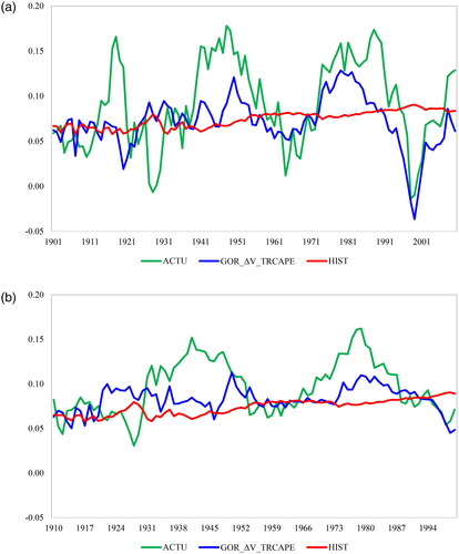
Figure 2. 10-Year and 20-Year Forecast Errors

Notes. (a) Forecast errors for 10-year forecasts based on the three-component approach with the TRCAPE proxy for ΔV, along with forecast errors for the historical mean model. (b) Forecast errors for 20-year forecasts based on the three-component approach with the TRCAPE proxy for ΔV, along with forecast errors for the historical mean model.

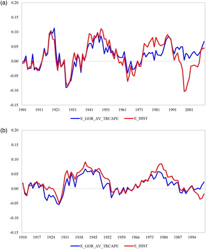
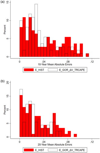
Figure 3. 10-Year and 20-Year Absolute Forecast Errors

Notes. (a) Distributions of absolute forecast errors for two models: the three-component model with the TRCAPE proxy for ΔV (depicted as transparent rectangles with black outlines) and the historical mean model (depicted in red). (b) Distributions of absolute forecast errors for two models: the three-component model with the TRCAPE proxy for ΔV (depicted as transparent rectangles with black outlines) and the historical mean model (depicted in red).

In Table 3, we report equivalent results for a 20-year forecast period. The MAEs are considerably lower for the 20-year forecast period compared to the 10-year forecast period. For instance, the average 20-year forecast period MAE for the 1988–2020 period is just 0.0155, compared to 0.0423 for the 10-year forecast. This is consistent with the results in Table 1 Panel C, which show lower standard deviations for 20-year returns. Furthermore, the gains over the historical mean approach are also generally greater for 20-year predictions than for 10-year predictions. For instance, over the entire sample period, the MAE improvement for the three-component model based on TRCAPE for 20-year intervals is 19.79% as compared to 16.35% for 10-year intervals. Moreover, the OOS-R² is generally greater. The three-component model with valuation changes determined by TRCAPE generates an OOS-R² of 37.23% for the entire period for 20-year predictions as compared to 30.51% for 10-year forecast results.

Table 3. 20-Year Forecasts

	1891–2020			1955–2020			1988–2020
	MAE	MAE Diff.	OOS-R^2	MAE	MAE Diff.	OOS-R^2	MAE	MAE Diff.	OOS-R^2
[1] Historical Mean	0.0282	0.0000	0.00%	0.0256	0.0000	0.00%	0.0129	0.0000	0.00%
Panel A: Yield Alone, YLDi
[2] YLDDiv	0.0291	−0.0014	12.00%**	0.0251	−0.0005	7.01%	0.0084	−0.0045*	56.96%*
[3] YLDTtl	0.0275	−0.0029	17.63%**	0.0246	−0.0010	9.84%*	0.0071	−0.0058*	66.45%*
[4] YLDNTtl	–	–	–	0.0182	−0.0073*	49.69%**	0.0126	−0.0003	−1.49%*
[5] YLDCATY	0.0285	−0.0019	12.06%**	0.0252	−0.0004	5.87%	0.0102	−0.0027**	38.26%*
Panel B: Gordon, GORi,j = YLDi + gj
[6] GORDiv,E = YLDDiv + gE	0.0320	0.0038	−13.79%	0.0311	0.0055	−19.79%	0.0138	0.0009	5.40%*
[7] GORDiv,Div = YLDDiv + gDiv	0.0326	0.0044	−14.89%	0.0335	0.0080	−35.78%	0.0166	0.0037	−26.05%*
[8] GORTtl,Ttl = YLDTtl + gTtl	0.0317	0.0035	−13.48%	0.0314	0.0059	−26.57%	0.0108	−0.0021	36.82%*
[9] GORNTtl,Ttl = YLDNTtl + gTtl	0.0468	0.0122	−38.06%	0.0446	0.0191	−111.64%	0.0293	0.0164	−292.82%*
[10] GORCATY,CATY = YLDCATY + gCATY	0.0338	0.0056	−27.68%	0.0335	0.0080	−45.88%	0.0118	−0.0011	25.30%*
Panel C: Valuation Alone, ΔVk
[11] ΔVTRCAPE	0.0257	−0.0048**	31.64%**	0.0213	−0.0042	40.58%**	0.0167	0.0037	−76.68%*
[12] ΔVBUF	0.0227	−0.0026	27.00%**	0.0228	−0.0028	27.39%**	0.0066	−0.0064*	73.57%*
[13] ΔVCON	–	–	–	–	–	–	0.0316	0.0154	−202.83%
Panel D: Three Components, GORDiv,Div + ΔVk
[14] GORDiv,Div + ΔVTRCAPE	0.0248	−0.0056	37.23%**	0.0183	−0.0073**	51.45%**	0.0086	−0.0043	57.05%
[15] GORDiv,Div + ΔVBUF	0.0205	−0.0048	41.91%*	0.0203	−0.0052	43.33%*	0.0076	−0.0053	66.95%*
[16] GORDiv,Div + ΔVCON	–	–	–	–	–	–	0.0302	0.0140	−179.67%

MAE = mean absolute error; OOS = out-of-sample.

Notes. This table reports results for 20-year forecasts over the entire sample period as well as half and quarter sub-periods. MAE is the mean absolute difference between the forecast and actual returns. MAE Diff. is the difference in MAEs between each prediction model and the historical mean model. We measure the statistical significance of MAE Diff. using the moving block bootstrap method, which accounts for autocorrelation in the time series. For each prediction model, we generate 1,000 bootstrap resamples and report statistical significance based on the one-sided bootstrap p value. We also use the moving block bootstrap method in determining the statistical significance of the differences in MAEs across our prediction models. MAEs in bold are MAEs of Tier 1 models with the lowest MAEs. ** and * indicate the significance levels of 1% and 5%, respectively.

As highlighted in bold in Table 3, the MAEs of several models within each framework are not statistically distinguishable from each other. However, as with 10-year interval forecasts, we concentrate on the three-component model with valuation changes determined by TRCAPE, as we consider this model the best performer across all evaluated metrics, including asset allocation. During the periods of 1891–2020, 1955–2020, and 1988–2020, the model generates $R_{\mathit{\text{OOS}}}^2$ improvements of 37.23%, 51.45%, and 57.05%, respectively. Figures 1b, 2b, and 3b depict the forecasted returns, forecast errors, and absolute forecast errors of this model and the historical mean model.

Wolf (2000) advocates a statistical method based on block bootstrapping to generate confidence intervals for regression parameters under three situations where the ordinary least squares inference is invalid. The first is in a long-horizon predictive regression in which the residuals are correlated. The second is in a regression with predetermined but endogenous independent variables, as discussed by Stambaugh (1986). The third is a situation in which there is positive skewness in the finite-sampling distribution of estimated predictive coefficients, as documented by Goetzmann and Jorion (1993). We, therefore, generate regression results based on the Wolf (2000) approach. This involves determining the optimal block bootstrap length, calibrating for the desired 95% confidence interval, and generating 1,000 bootstrap samples for each predictive regression model. As per Table 6 of Wolf (2000), we report the in-sample regression coefficient ${\widehat{\beta }}_k$ along with the 95% confidence intervals for the estimated coefficient ${\widehat{\beta }}_k.$ In Online Supplemental Appendix Table A2, Eq. (1)(1) $$r_{t:t+h}=\alpha +\beta x_t+{\epsilon }_{t:t+h} \mathrm{\text{for}}\mathrm{ }t=1,\dots ,T-h$$(1) is applied to models 1 to 7 and Eq. (2)(2) $$\Delta V_{t:t+h}=\gamma +\delta z_t+{\epsilon }_{t:t+h}\text{for}t=1,\dots ,T-h$$(2) is applied to models 8 to 10. Note that the Gordon model, based solely on the sum of yield and historical dividend growth, does not involve a predictive regression; hence, we are unable to include it in this framework.

Table A2 results indicate that each of the framework and proxy parameters, except for the valuation alone model based on CON and the three competent models including CON, are statistically significant for 10-year horizons. This is indicated by the fact that the upper and lower confidence bounds do not include zero. Furthermore, each of the framework and proxy parameters are statistically significant for 20-year horizons, except for the three-component model based on BUF. It is also important to note that long-horizon regressions face other challenges that are difficult to account for, such as surviving markets exhibiting mean reversion.

We also apply two alternative methods of determining the statistical significance of our results.⁹ First, we conduct simulations under the assumption of no return predictability where the return is simulated independently and is unrelated to the predictors. We simulate predictors based on their means, standard deviations, and correlations among the existing predictors. We then simulate monthly log returns from a normal distribution with the same mean and variance as the actual monthly log returns and calculate simulated overlapping 10- and 20-year returns. This process is repeated 1,000 times to construct 1,000 simulated samples.

We then run the exact exercise performed earlier in this paper and present the 95% confidence intervals for the MAEs and OOS-R² values among the 1,000 simulated samples. If the predictability results of a given framework hold, we would expect the MAEs of that framework in Tables 2 or 3 to be lower than the lower limit of the 95% MAE confidence interval and the OOS-R² to be above the upper limit of the 95% OOS-R² confidence interval. We find that this is the case for the best frameworks and input proxies. For instance, in Table 3, the full-sample results for the three-component model with valuation change based on TRCAPE show an MAE of 0.0248, which is below 0.0268 in Panel B of Online Supplemental Appendix Table A3. Similarly, the OOS-R² of 37.23% exceeds 2.66% in Panel B of Table A3. Therefore, the 20-year return predictability for this three-component model is robust, based on our simulation results.

Second, we conduct simulations under return predictability. We assume that the return-generating process follows the linear regression estimates between the return and its predictor. We further assume an AR(1) process for the error term: $e_t=c_1\times e_{t-1}+v_t,$ where $c_1$ represents the autocorrelation of actual predictive model residuals, calculated using real data, and $v_t$ is simulated from a normal distribution with a mean of zero and the same variance as the actual model residuals. This analysis illustrates the out-of-sample performance of the correctly specified regression analysis. We present the results in Online Supplemental Appendix Table A4.

Table 4. Mean Absolute Errors in Different Market States

	10-Year Forecasts				20-Year Forecasts
	Return	Volatility	Amihud	Recession	Return	Volatility	Amihud	Recession
Panel A: Yield Alone, YLDi
YLDDiv	0.3597**	−0.1742*	−0.128	−0.0264	0.6678**	−0.3508**	0.1513	−0.0328
YLDTtl	0.3453**	−0.1515*	−0.0523	−0.0090	0.6543**	−0.3529**	0.1362	−0.0122
YLDNTtl	0.3681**	−0.2419**	1.9298**	0.0352	0.4211**	−0.4575**	−0.3971	−0.0571
YLDCATY	0.3455**	−0.1523	−0.0512	0.0150	0.6620**	−0.3511**	0.1448	−0.0387
Panel B: Gordon, GORi,j = YLDi + gj
GORDiv,E = YLDDiv + gE	0.3418**	−0.1640	−0.0834	−0.0218	0.6437**	−0.3049**	0.1918	−0.0155
GORDiv,Div = YLDDiv + gDiv	0.3632**	−0.1739*	−0.1129	−0.0234	0.6604**	−0.3530**	0.0797	−0.0397
GORTtl,Ttl = YLDTtl + gTtl	0.3656**	−0.1695*	−0.0764	−0.0070	0.6964**	−0.4114**	0.0489	−0.0186
GORNTtl,Ttl = YLDNTtl + gTtl	0.5573**	−0.3121**	−0.2384	−0.0657	0.6105**	−0.4293**	−0.0477	−0.0434
GORCATY,CATY = YLDCATY + gCATY	0.3701**	−0.1761*	−0.0608	−0.0041	0.7309**	−0.4088**	0.0912	−0.0242
Panel C: Valuation Alone, ΔVk
ΔVTRCAPE	0.2608**	−0.0962	−0.1335	−0.0469	0.5284**	−0.2817**	0.0916	−0.0303
ΔVBUF	0.3612**	−0.3817**	−0.0165	−0.1594**	0.5898**	−0.6623**	0.0737	−0.0629
ΔVCON	0.2255	−0.192	9.2521	0.0144	0.3495	0.7750	11.9036	−1.8281**
Panel D: Three Components, GORDiv,Div + ΔVk
GORDiv,Div + ΔVTRCAPE	0.1708	−0.0071	0.0942	0.0099	0.3774**	−0.1098	0.3130**	0.0801
GORDiv,Div + ΔVBUF	0.2814**	−0.3210**	0.2089	−0.1498**	0.4500**	−0.5137**	0.3743	0.0286
GORDiv,Div + ΔVCON	0.2190	−0.1949	8.7832	0.0154	0.6304*	1.2579*	19.0762*	−1.2821*

MAE = mean absolute error; OOS = out-of-sample.

Notes. This table displays MAEs in different market states. For each prediction model, we run the following time-series regression with Newey–West (1987) standard errors: ${\mathit{\text{MAE}}}_{i,t}={\alpha }_i+{\beta }_i{\mathit{\text{MKT}}\_\mathit{\text{STATE}}}_t+{\epsilon }_{i,t},$ where MAE_i is the 10- or 20-year mean absolute errors for prediction model i and MKT_STATE is one of our four market state proxies, calculated over the same 10- or 20-year period as MAE_i. The four market state proxies include market return, market volatility, market Amihud (2002) ratio, and market recession. Market return and the Amihud (2002) ratio are the average annual market return and the average annual value-weighted stock Amihud (2002) ratio, respectively. Market volatility is the standard deviation of annual returns over the same period as MAE_i. The market recession proxy is determined by calculating the proportion of months (within a 10- or 20-year period) that fall within the recessionary phases of the National Bureau of Economic Research business cycle. ** and * indicate the significance levels of 1% and 5%, respectively.

For models 1 to 4 and 10 to 15 in Table A4 (Online Supplemental Appendix), we use historical data to run the predictive regression, obtaining the in-sample intercept and slope. With the estimated intercepts, slopes, actual predictors, and simulated $e_t$ values, we simulate 10-year and 20-year overlapping returns for each model. This process is repeated to construct 1,000 simulated samples for each model. Table A4 presents the 95% confidence intervals for the MAEs and OOS-R² values among these 1,000 simulated samples.

The results in Table A4 highlight several models with a negative OOS-R² in Tables 2 and 3 that are in the range of correctly specified models under predictability. For instance, the OOS-R² for the YLD_Div model in Table 2 is –11.54%, which is within the 95% confidence interval in Panel A of Table A4. This raises the possibility that other models in Table 2 may warrant further consideration. This highlights the challenges involved in long-term predictability research.

Moreover, we generate results for a five-year forecast horizon and present these in Online Supplemental Appendix Table A5. The five-year horizon results indicate that there is less predictability on average than for the 10-year horizon. The five-year average MAE and OOS-R² are 0.0629 and 1.54%, compared to 0.0395 and 9.16%, respectively, for 10-year horizons. The three-component models and valuation alone models perform similarly well. The single best specification is valuation alone based on TRCAPE, although this is not statistically significantly superior to several other specifications.

Table 5. Asset Allocation 10-Year Forecasts

	1891–2020			1955–2020			1988–2020
	VaR	Alpha	Sharpe	VaR	Alpha	Sharpe	VaR	Alpha	Sharpe
[1] Historical Mean	−0.1621	0.0027	0.1933	−0.1912	0.0060	0.2618	−0.1912	0.0181	0.3181
Panel A: Yield Alone, YLDi
[2] YLDDiv	−0.0695**	0.0194**	0.3543*	−0.0695**	0.0173	0.3116	−0.0552	0.0332	0.4747
[3] YLDTtl	−0.1183*	0.0073	0.2457	−0.0838**	0.0143	0.3043	−0.0397	0.0288	0.4494
[4] YLDNTtl	−0.0869	0.0096	0.3521	−0.1449	0.0128	0.2829	−0.0781	0.0273	0.3726
[5] YLDCATY	−0.1128**	0.0050	0.2357	−0.1128**	0.0125	0.3031	−0.0368*	0.0252	0.4439
Panel B: Gordon, GORi,j = YLDi + gj
[6] GORDiv,E = YLDDiv + gE	−0.0828**	0.0102*	0.2618	−0.0882**	0.0195	0.3228	−0.0373	0.0423*	0.5045
[7] GORDiv,Div = YLDDiv + gDiv	−0.0711**	0.0114	0.2691	−0.0752**	0.0227*	0.3489	−0.0477	0.0469*	0.5500
[8] GORTtl,Ttl = YLDTtl + gTtl	−0.0862**	0.0104**	0.2862*	−0.0748**	0.0152	0.3192	−0.0319*	0.0286	0.4617
[9] GORNTtl,Ttl = YLDNTtl + gTtl	−0.0826	0.0093	0.2541	−0.0781**	0.0144	0.2723	−0.0781	0.0288	0.4005
[10] GORCATY,CATY = YLDCATY + gCATY	−0.0660**	0.0104*	0.2721	−0.0698**	0.0210*	0.3630	−0.0319*	0.0411*	0.5675
Panel C: Valuation Alone, ΔVk
[11] ΔVTRCAPE	−0.0789**	0.0126	0.2751	−0.0947**	0.0150	0.2759	−0.0781	0.0358	0.4278
[12] ΔVBUF	−0.0688**	0.0332**	0.4393	−0.0688**	0.0284*	0.3368	−0.0781	0.0481*	0.4366
[13] ΔVCON	–	–	–	−0.2045	−0.0014	0.2810	−0.2045	0.0037	0.2756
Panel D: Three Components, GORDiv,Div + ΔVk
[14] GORDiv,Div + ΔVTRCAPE	−0.0781*	0.0171*	0.3108	−0.0781**	0.0182	0.3057	−0.0414	0.0449*	0.5311
[15] GORDiv,Div + ΔVBUF	−0.0624**	0.0357**	0.4549	−0.0743**	0.0300*	0.3477	−0.0781	0.0474*	0.4290
[16] GORDiv,Div + ΔVCON	–	–	–	−0.1100	0.0119	0.3701	−0.1100	0.0165	0.3639

VaR, value at risk; OOS = out-of-sample.

Notes. This table compares different models from an asset allocation perspective for 10-year forecasts. We allocate the portfolio between stocks and bonds using data on the S&P 500 Index and the US 10-year government bond total return index. We employ the mean-variance approach and consider optimal portfolio weights as the asset weights that maximize the portfolio Sharpe ratio. Following the derivation in Smith (2019), we calculate optimal weights and rebalance the portfolio annually, based on the expected Sharpe ratios of the two assets, their historical standard deviations, and the historical correlation between them. To calculate the expected Sharpe ratio, [E(R) – R_f]/σ, for the S&P 500 (which serves as one input for determining optimal portfolio weights), we use our OOS S&P 500 return forecasts from each of our prediction models, historical risk-free rates sourced from the updated Goyal and Welch (2008) dataset, and historical standard deviations of S&P 500 returns. Accordingly, optimal weights and realized portfolio returns differ across our models. We then generate three performance metrics for realized portfolio returns: 5% VaR, ex post alpha (Alpha), and ex post Sharpe ratio (Sharpe). We employ the aforementioned moving block bootstrap approach to bootstrap realized portfolio returns and determine whether the realized VaR of portfolios constructed based on each of our prediction models is significantly lower than that based on the historical mean model. Similarly, we also examine whether the realized alpha and Sharpe ratio of portfolios based on our prediction models are significantly higher than those based on the historical mean model. ** and * indicate the significance levels of 1% and 5%, respectively.

Table 6. Asset Allocation 20-Year Forecasts

	1891–2020			1955–2020			1988–2020
	VaR	Alpha	Sharpe	VaR	Alpha	Sharpe	VaR	Alpha	Sharpe
[1] Historical Mean	−0.1344	−0.0021	0.2040	−0.1053	0.0025	0.3025	−0.1053	−0.0009	0.5063
Panel A: Yield Alone, YLDi
[2] YLDDiv	−0.1046	0.0039	0.2581	−0.0867**	0.0032	0.3018	−0.0722*	0.0047	0.5353
[3] YLDTtl	−0.1087	0.0043	0.2608	−0.0846**	0.0031	0.2956	−0.0674*	0.0051	0.5337
[4] YLDNTtl	–	–	–	−0.0999	0.0101	0.3348	−0.0683	0.0372	0.6400
[5] YLDCATY	−0.1046	0.0032	0.2517	−0.0912**	0.0025	0.2980	−0.0912	0.0006	0.5121
Panel B: Gordon, GORi,j = YLDi + gj
[6] GORDiv,E = YLDDiv + gE	−0.0774**	0.0052	0.2495	−0.0774*	0.0076	0.3046	−0.0373	0.0202	0.5365
[7] GORDiv,Div = YLDDiv + gDiv	−0.0752**	0.0058	0.2504	−0.0752*	0.0102	0.3161	−0.0493	0.0252	0.5309
[8] GORTtl,Ttl = YLDTtl + gTtl	−0.0748*	0.0082*	0.2794	−0.0690**	0.0085	0.3137	−0.0319	0.0160	0.5323
[9] GORNTtl,Ttl = YLDNTtl + gTtl	−0.0826	0.0052	0.2471	−0.0656*	0.0088	0.2625	−0.0781	0.0242	0.4561
[10] GORCATY,CATY = YLDCATY + gCATY	−0.0698**	0.0061	0.2529	−0.0698**	0.0115	0.3311	−0.0319	0.0234	0.5558
Panel C: Valuation Alone, ΔVk
[11] ΔVTRCAPE	−0.1046	0.0058	0.2623	−0.0846*	0.0060	0.2957	−0.0781	0.0284	0.5233
[12] ΔVBUF	−0.1083	0.0079	0.3544	−0.1083	0.0082	0.3301	−0.0319*	0.0264	0.6211
[13] ΔVCON	–	–	–	–	–	–	−0.0257*	0.0341*	0.7264*
Panel D: Three Components, GORi,j + ΔVk
[14] GORDiv,Div + ΔVTRCAPE	−0.1046	0.0184	0.3669	−0.0920*	0.0059	0.3123	−0.0319	0.0380	0.6897
[15] GORDiv,Div + ΔVBUF	−0.0806*	0.0056	0.3460	−0.0806*	0.0052	0.3145	−0.0319	0.0259	0.6515
[16] GORDiv,Div + ΔVCON	–	–	–	–	–	–	−0.0093*	0.0405	0.7753

VaR, value at risk; OOS = out-of-sample.

Notes. This table compares different models from an asset allocation perspective for 20-year forecasts. We allocate the portfolio between stocks and bonds using data on the S&P 500 Index and the US 10-year government bond total return index. We employ the mean-variance approach and consider optimal portfolio weights as the asset weights that maximize the portfolio Sharpe ratio. Following the derivation in Smith (2019), we calculate optimal weights and rebalance the portfolio annually, based on the expected Sharpe ratios of the two assets, their historical standard deviations, and the historical correlation between them. To calculate the expected Sharpe ratio, [E(R) – R_f]/σ, for the S&P 500 (which serves as one input for determining optimal portfolio weights), we use our OOS S&P 500 return forecasts from each of our prediction models, historical risk-free rates sourced from the updated Goyal and Welch (2008) dataset, and historical standard deviations of S&P 500 returns. Accordingly, optimal weights and realized portfolio returns differ across our models. We then generate three performance metrics for realized portfolio returns: 5% VaR, ex post alpha (Alpha), and ex post Sharpe ratio (Sharpe). We employ the aforementioned moving block bootstrap approach to bootstrap realized portfolio returns and determine whether the realized VaR of portfolios constructed based on each of our prediction models is significantly lower than that based on the historical mean model. Similarly, we also examine whether the realized alpha and Sharpe ratio of portfolios based on our prediction models are significantly higher than those based on the historical mean model. ** and * indicate the significance levels of 1% and 5%, respectively.

Taken together, results for different forecasting horizons indicate that predictability is strongest for 20-year horizons, followed by 10-year horizons, and weakest for 5-year horizons. Investigating the reasons for this is beyond the scope of this research, but we conjecture that the predictors might better forecast the longer horizon return because it is less volatile and less noisy compared to the shorter horizon return. Also, shorter horizon returns may be more heavily influenced by a major and hard-to-foresee economic shock such as the Great Depression, the Oil Shock, or the global financial crisis.

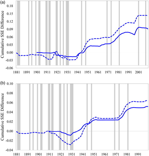
We present graphs along the lines of Goyal and Welch (2008) in Figures 4a and 4b, which plot the in-sample and out-of-sample performance for the top 10-year and 20-year forecast performers. These relate to the three-component model with valuation changes based on TRCAPE. The performance is measured based on the difference in cumulative squared prediction errors between the historical mean model and our top 10-year or 20-year forecast performers. An increase in the lines indicates better performance of the top forecast performers relative to the historical mean model. Recession periods are marked with grey bars. Figures 4a and 4b indicate that the three-component model with valuation changes based on TRCAPE began adding value to investors around 1940 and has performed well since.

Figure 4. 10-Year and 20-Year Forecast Performance Gain

Notes. (a) Following the approach of Goyal and Welch (2008), the dotted and solid lines in this figure represent the in-sample and out-of-sample 10-year forecast performance, respectively, of the three-component model with the TRCAPE proxy for ΔV. An increase in the lines indicates better performance of this three-component model relative to the historical mean model. If 75% or more of a year falls within National Bureau of Economic Research recession periods, those years are marked by grey vertical lines. (b) Following the approach of Goyal and Welch (2008), the dotted and solid lines in this figure represent the in-sample and out-of-sample 20-year forecast performance, respectively, of the three-component model with the TRCAPE proxy for ΔV. An increase in the lines indicates better performance of this three-component model relative to the historical mean model. If 75% or more of a year falls within National Bureau of Economic Research recession periods, those years are marked by grey vertical lines.

Prior studies show that return predictability is time-varying (e.g., Devpura, Narayan, and Sharma 2018; Jurdi 2022). In Table 4, we report the MAEs in different market states over time. For each prediction model, we run the following time-series regression with Newey–West (1987) standard errors: (4) $${\mathit{\text{MAE}}}_{i,t}={\alpha }_i+{\beta }_i{\mathit{\text{MKT}}\_\mathit{\text{STATE}}}_t+{\epsilon }_{i,t}$$(4) where MAE_i is the 10- or 20-year MAEs for prediction model i and MKT_STATE is one of our four market state proxies, calculated over the same 10- or 20-year period as MAE_i. The four market state proxies include market return, market volatility, the Amihud (2002) illiquidity ratio, and a market recession indicator. Market return and the Amihud (2002) ratio are the average annual market return and the average annual value-weighted stock Amihud (2002) ratio, respectively. Market volatility is the standard deviation of annual returns over the same period as MAE_i. The market recession proxy is determined by calculating the proportion of months (within a 10- or 20-year period) that fall within the recessionary phases of the National Bureau of Economic Research business cycle.

The results in Table 4 indicate that forecasts tend to be more accurate (i.e., MAEs are lower) when returns are lower. Furthermore, forecasts are more accurate when volatility is higher. There is no consistent relation between forecast accuracy and liquidity or the business cycle. The business cycle result differs from shorter horizon predictability, which is stronger in economic contractions (e.g., Henkel, Martin, and Nadari 2011). In Online Supplemental Appendix A6, we generate results using mean squared errors as the dependent variable. These are very similar to the results in Table 4.

In Tables 5 and 6, we compare the different models from an asset allocation perspective. We allocate the portfolio between stocks and bonds using data on the S&P 500 Index and the US 10-year government bond total return index. We employ the mean-variance approach and consider optimal portfolio weights as the asset weights that maximize the portfolio Sharpe ratio. Following the derivation in Smith (2019), we calculate optimal weights and rebalance the portfolio annually based on the expected Sharpe ratios of the two assets, their historical standard deviations, and the historical correlation between them. To calculate the expected Sharpe ratio, $\left[E\left(R\right)-R_f\right]/\sigma ,$ for the S&P 500 (which serves as one input for determining optimal portfolio weights), we use our OOS S&P 500 return forecasts from each of our prediction models (i.e., E(R)), historical risk-free rates sourced from the updated Goyal and Welch (2008) dataset (i.e., R_f), and historical standard deviations of S&P 500 returns (i.e., σ). Accordingly, optimal weights and realized portfolio returns differ across our models in Tables 5 and 6.

We then generate three performance metrics for realized portfolio returns: 5% value at risk (VaR), ex post alpha (alpha), and ex post Sharpe ratio (Sharpe). We employ the aforementioned moving block bootstrap approach to bootstrap realized portfolio returns and determine whether the realized VaR of portfolios constructed based on each of our prediction models is significantly improved compared to the historical mean model. Similarly, we also examine whether realized alpha values and Sharpe ratios of portfolios based on our prediction models are significantly higher than those based on the historical mean model.

The results in Table 5 indicate that there are important gains from an asset allocation perspective. For instance, for the entire period, the VaR for the three-component model with TRCAPE valuation changes is −7.81%, compared to −16.21% for the historical mean model. Furthermore, the Sharpe ratio of this model is 0.3108, compared to 0.1933 for the historical mean model. These results are not specific to the entire period. For the more recent period of 1988–2020, the VaR for the three-component model with TRCAPE valuation changes is −4.14%, compared to −19.12% for the historical mean model. The alpha for this model for the most recent period is 4.49%, compared to 1.81% for the historical mean model.

Strong gains from an asset allocation perspective are also evident in the 20-year forecast results, as shown in Table 6. The three-component model with valuation changes determined by TRCAPE generates a Sharpe ratio of 0.3669 for the entire period, compared to 0.2040 for the historical mean model. The Sharpe ratio generated by this model is also larger than that of the historical mean model in each of the two most recent periods, but the differences are not statistically significant. However, the three-component model with valuation changes determined by TRCAPE exhibits significantly superior VaRs in both recent periods when compared to the historical mean model. For instance, the VaR of this model stands at just −3.19% in the 1988–2020 period, compared to −10.53% for the historical mean model.

In Online Supplemental Appendix Figures A1a and A1b, we present the time variation in the weights allocated to stocks for the three-component model with valuation changes based on TRCAPE for both the 10-year and 20-year forecast horizons. These indicate that there is almost no allocation to stocks before 1937. From 1937 onward, there is a time-varying but consistently positive weight to stocks until 1981. This was then followed by a period of positive weights through the mid-1990s.

We present summary statistics for stock weights in Panels A and B of Table 7. For 10-year forecast horizons, the average stock weight is 47.02% across all periods. The average is higher during expansionary periods (50.63%) than during recessionary periods (30.77%). The difference in median stock weights is even more pronounced: The median stock weight in recessions is 2.50%, whereas it is 51.54% in expansions. The difference between stock weights across recessions and expansions is even greater for 20-year forecast intervals. The mean stock weight across the entire sample is 59.32%. However, this is just 29.07% in recessions compared to 65.77% in expansions. The results in Panel B indicate that the stock weight is often 0% or 100%. There is a marked difference in the frequency of a 0% weight in 20-year forecasts: 68.75% during recessions, but only 24% during expansions.

Table 7. Portfolio Stock Weights

Panel A: Summary Statistics on Stock Weights
		10-Year Forecasts			20-Year Forecasts
		Full Sample	Recession	Expansion	Full Sample		Recession	Expansion
Mean		47.02%	30.77%	50.63%	59.32%		29.07%	65.77%
Std Dev		43.39%	43.22%	42.83%	44.73%		45.25%	42.17%
Min		0.00%	0.00%	0.00%	0.00%		0.00%	0.00%
Median		39.54%	2.50%	51.54%	80.27%		0.00%	85.55%
Max		100.00%	100.00%	100.00%	100.00%		100.00%	100.00%
Panel B: Proportions of Stock Weights
		10-Year Forecasts			20-Year Forecasts
		Full Sample	Recession	Expansion	Full Sample		Recession	Expansion
Weight = 0%		33.64%	50.00%	30.00%	31.87%		68.75%	24.00%
0% < Weight < 20%		7.27%	15.00%	5.56%	2.20%		0.00%	2.67%
20% < Weight < 40%		9.09%	5.00%	10.00%	2.20%		0.00%	2.67%
40% < Weight < 60%		7.27%	5.00%	7.78%	1.10%		0.00%	1.33%
60% < Weight < 80%		7.27%	0.00%	8.89%	10.99%		6.25%	12.00%
80% < Weight < 100%		5.45%	0.00%	6.67%	13.19%		0.00%	16.00%
Weight = 100%		30.00%	25.00%	31.11%	38.46%		25.00%	41.33%
Panel C: Summary Statistics on Duration (Years)
	10-Year Forecasts				20-Year Forecasts
	< 60%	> 60%	= 0%	= 100%	< 60%	> 60%	= 0%	= 100%
Mean	7.88	6.71	7.40	4.71	8.50	19.00	14.50	5.83
Std Dev	10.62	4.46	6.47	3.04	13.08	13.45	19.09	5.19
Min	1.00	1.00	1.00	1.00	1.00	8.00	1.00	1.00
Median	2.50	7.00	6.00	4.00	2.50	15.00	14.50	4.50
Max	31.00	14.00	16.00	9.00	28.00	34.00	28.00	14.00

Notes. In Panels A and B, we present summary statistics on weights allocated to stocks for the three-component model with the TRCAPE proxy for the 10-year and 20-year forecast horizons. In Panel C, we present summary statistics for the duration in years that different weights are maintained.

In Panel C, we present summary statistics for the duration, in years, that different weights are maintained. The results indicate that the weights are strongly persistent. For instance, weights of less than 60% are maintained for more than seven years on average, while weights of greater than 60% are maintained for more than 6 years. These durations are even longer for 20-year forecast horizons: On average, weights of greater than 60% are maintained for 19 years.

Conclusions

Accurately estimating long-term expected returns of equity markets is important for both corporate entities and individual investors. We investigate the ability of different frameworks and input proxies to estimate 10- and 20-year OOS returns over long historical periods and more recent periods. We document that the best approach is the three-component model, based on dividend yield, growth, and valuation from the TRCAPE ratio. This generates meaningful improvements compared to historical mean model forecasts. OOS-R² can be as significant as 30% even in the most recent period, and asset allocation based on our model forecasts can improve a portfolio’s Sharpe ratio and VaR by more than 50%. We hope that our results are of interest to those who require accurate long-term expected return forecasts.

Acknowledgments

We thank seminar participants at Massey University, La Trobe University, ACC Investment Management, and the New Zealand Finance Colloquium; our editors William Goetzmann and Luis Garcia-Feijo, CFA, CIPM; and two anonymous referees for their valuable comments. This paper won the CFA-ARX Best Paper award at the 2024 New Zealand Finance Colloquium. All errors are our own.

Disclosure Statement

No potential conflict of interest was reported by the author(s).

Additional information

Notes on contributors

Rui Ma

Rui Ma is a lecturer in finance at La Trobe Business School, La Trobe University, Melbourne, Australia.

Ben R. Marshall

Ben R. Marshall is the MSA Charitable Trust Professor of Finance in the School of Economics and Finance, Massey Business School, Massey University, Palmerston North, New Zealand.

Nhut H. Nguyen

Nhut H. Nguyen is a professor of finance in the Department of Economics and Finance, Auckland University of Technology, Auckland, New Zealand.

Nuttawat Visaltanachoti

Nuttawat Visaltanachoti, CFA, is the dean’s chair professor of finance in the School of Economics and Finance, Massey Business School, Massey University, Auckland, New Zealand.

Notes

1 Long-term return forecasts are more relevant to a range of stakeholders, including investors, businesses, and governments. However, data limitations present econometric issues that have impacted this literature (e.g., Boudoukh, Israel, and Richardson 2022). It is therefore unsurprising that most return predictability literature has focused on monthly return predictability (e.g., Rapach, Ringgenberg, and Zhou 2016).

2 Campbell and Shiller (1998) also use the dividend-to-price ratio as a valuation ratio. We adopt the Gordon growth framework and thus classify this as “yield alone” rather than “valuation alone,” but this classification has no impact on the reported results.

3 Boudoukh, Israel, and Richardson (2022) propose an in-sample approach that is free from overlapping sample bias. However, we do not apply this, as a large focus of our work is to compare the performance of various predictive approaches, and this is more readily achieved in an OOS setting.

4 In unreported results, we also follow Damodaran (2022) and calculate growth as being equal to the risk-free rate. This method does not have a material impact on our key conclusions. Golez and Koudijs (2023) highlight the link between the market payout ratio and dividend growth. We, therefore, regress the average dividend growth rate over the next 10- and 20-year horizons on the current payout ratio, defined as dividends divided by earnings. We then use the estimated regression coefficients, along with the most recent payout ratio to forecast the future OOS dividend growth rate and use this growth estimate in the Gordon growth model. The unreported results are consistent with those based on the historical average growth rate. We thank an anonymous referee for suggesting this analysis to us.

5 We thank Robert Shiller for making these data available: http://www.econ.yale.edu/∼shiller/data.htm.

6 In an earlier version of this paper, we also included the total wealth portfolio composition (WPC), which measures the value of stock market wealth relative to the value of other assets including residential housing and government bonds. High WPC ratios predict low future stock market returns (e.g., Rintamaki 2023). However, an anonymous referee brought our attention to Eichholtz et al. (2021), who raise concerns about the Jordà-Schularick-Taylor Macrohistory real estate series upon which our WPC measure was based. We were not able to source an alternative real estate wealth series, so we remove WPC from our analysis. Given that WPC was a component of the average valuation proxies included in an earlier version, we also remove them in the current version.

7 We believe that MAEs better reflect the performance of a forecast than correlations, as they account for the magnitude of errors between forecasted and actual returns. We provide an example in Online Supplemental Appendix Table A1 of a scenario in which one forecast can have a larger correlation than another forecast (indicating outperformance) and also have a larger MAE (indicating underperformance).

8 In Tables 2 and 3, the values in bold are MAEs of Tier 1 models, which have the lowest MAEs.

9 We thank an anonymous referee for suggesting this analysis to us.

Appendix 1

Predictor Description

Table

Model	Description
Historical Mean	Historical average return on the S&P 500 Index is used as the forecast.
YLDDiv	We use the log dividend yield (e.g., Ferreira and Santa-Clara, 2011; Rapach, Ringgenberg, and Zhou, 2016) as the predictor to compute a standard predictive regression forecast. Dividend yield in year t is calculated as dividend in year t divided by the S&P 500 Index value at the end of year t − 1.
YLDTtl	We use the log total yield as the predictor to compute a standard predictive regression forecast. Total yield is the dividend yield plus the buyback yield as per Straehl and Ibbotson (2017).
YLDNTtl	We use the log net total yield as the predictor to compute a standard predictive regression forecast. Net total yield is the dividend yield less net issuance as per Straehl and Ibbotson (2017).
YLDCATY	We use the cyclically adjusted total yield (CATY) as the predictor to compute a standard predictive regression forecast. CATY is computed as per Straehl and Ibbotson (2017).
GORDiv,E = YLDDiv + gE	The Gordon growth model with log dividend yield and average historical growth in earnings is used to compute a return forecast.
GORDiv,Div = YLDDiv + gDiv	The Gordon growth model with log dividend yield and average historical growth in dividends is used to compute a return forecast.
GORTtl,Ttl = YLDTtl + gTtl	The Gordon growth model with log total yield and average historical total yield growth is used to compute a return forecast. To calculate average historical total yield growth, we first multiply yearly total yield in year t by the S&P 500 Index value at the end of year t − 1, and then we calculate the average historical growth rate in the resulting time series.
GORNTtl,Ttl = YLDNTtl + gTtl	The Gordon growth model with log net total yield and average historical total yield growth is used to compute a return forecast.
GORCATY,CATY = YLDCATY + gCATY	The Gordon growth model with CATY and average historical CATY growth is used to compute a return forecast. To calculate average historical CATY growth, we first multiply yearly CATY in year t by the S&P 500 Index value at the end of year t − 1, and then we calculate the average historical growth rate in the resulting time series.
ΔVTRCAPE	We use the total return cyclically adjusted price-to-earnings ratio (TRCAPE) as the predictor to compute a standard predictive regression forecast. The TRCAPE data are sourced from the Shiller website: http://www.econ.yale.edu/∼shiller/data.htm
ΔVBUF	We use the Buffett indicator, the equity market capitalization scaled by gross domestic product, as the predictor to compute a standard predictive regression forecast.
ΔVCON	We use the detrended cyclical consumption as the predictor to compute a standard predictive regression forecast (e.g., Atanasov, Møller, and Priestley, 2020). We detrend consumption data in quarter q as per Eq. (2) of Atanasov, Møller, and Priestley (2020), and we use only the data available up to quarter q to avoid look-forward bias from the detrending process.
GORDiv,Div + ΔVTRCAPE	The return forecast is the sum of the Gordon growth model (with dividend yield and dividend growth) forecast and expected change in valuations. We use TRCAPE as the predictor to forecast the OOS change in valuations. The TRCAPE data are sourced from the Shiller website: http://www.econ.yale.edu/∼shiller/data.htm
GORDiv,Div + ΔVBUF	The return forecast is the sum of the Gordon growth model (with dividend yield and dividend growth) and expected change in valuations. We use the Buffett indicator, the equity market capitalization scaled by gross domestic product, as the predictor to forecast the OOS change in valuations.
GORDiv,Div + ΔVCON	The return forecast is the sum of the Gordon growth model (with dividend yield and dividend growth) and expected change in valuations. We use the detrended cyclical consumption (e.g., Atanasov, Møller, and Priestley, 2020) as the predictor to forecast the OOS change in valuations. We detrend consumption data in quarter q as per Eq. (2) of Atanasov, Møller, and Priestley (2020), and we use only the data available up to quarter q to avoid look-forward bias from the detrending process.

We conduct an ordinary least squares (OLS) out-of-sample (OOS) forecasting approach (e.g., Goyal and Welch, 2008). All OOS forecasts use only the data available up to the year in which the forecast is calculated.

References

- Amihud, Yakov. 2002. “Illiquidity and Stock Returns: Cross–Section and Time–Series Effects.” Journal of Financial Markets 5 (1): 31–56. doi:10.1016/S1386-4181(01)00024-6.
- Arnott, Robert D., Denis B. Chaves, and Tzee–man Chow. 2017. “King of the Mountain: The Shiller P/E and Macroeconomic Conditions.” The Journal of Portfolio Management 44 (1): 55–68. doi:10.3905/jpm.2017.44.1.055.
- Atanasov, Victoria, Stig V. Møller, and Richard Priestley. 2020. “Consumption Fluctuations and Expected Returns.” The Journal of Finance 75 (3): 1677–713. doi:10.1111/jofi.12870.
- Bogle, John C. 1991a. “Investing in the 1990s.” Journal of Portfolio Management 17 (3): 5–14.
- Bogle, John C. 1991b. “Investing in the 1990s: Occam’s Razor Revisited.” Journal of Portfolio Management 18 (1): 88–91.
- Boudoukh, Jacob, Ronen Israel, and Matthew Richardson. 2022. “Biases in Long-Horizon Predictive Regressions.” Journal of Financial Economics 145 (3): 937–69. doi:10.1016/j.jfineco.2021.09.013.
- Boudoukh, Jacob, Matthew Richardson, and Robert F. Whitelaw. 2008. “The Myths of Long-Horizon Predictability.” Review of Financial Studies 21 (4): 1577–605. https://www.jstor.org/stable/40056862. doi:10.1093/rfs/hhl042.
- Campbell, John Y., and John H. Cochrane. 1999. “By Force of Habit: A Consumption-Based Explanation of Aggregate Stock Market Behavior.” Journal of Political Economy 107 (2): 205–51. https://www.jstor.org/stable/10.1086/250059. doi:10.1086/250059.
- Campbell, John Y., and Robert J. Shiller. 1988. “Stock Prices, Earnings, and Expected Dividends.” Journal of Finance 43 (3): 661–76. https://www.jstor.org/stable/2328190.
- Campbell, John Y., and Robert J. Shiller. 1998. “Valuation Ratios and the Long-Run Stock Market Outlook.” Journal of Portfolio Management 24 (2): 11–26.
- Chiang, I–Hsuan E., and Walker K. Hughen. 2017. “Do Oil Futures Prices Predict Stock Returns?” Journal of Banking & Finance 79:129–41. doi:10.1016/j.jbankfin.2017.02.012.
- Clark, Todd E., and Kenneth D. West. 2007. “Approximately Normal Tests for Equal Predictive Accuracy in Nested Models.” Journal of Econometrics 138 (1): 291–311. doi:10.1016/j.jeconom.2006.05.023.
- Cochrane, John H. 2008. “The Dog That Did Not Bark: A Defense of Return Predictability.” Review of Financial Studies 21 (4): 1533–75. doi:10.1093/rfs/hhm046.
- Damodaran, Aswath. 2022. “Equity Risk Premiums (ERP): Determinants, Estimation, and Implications.” SSRN Working Paper. https://ssrn.com/abstract=4066060.
- Devpura, Neluka, Pareshm K. Narayan, and Susan S. Sharma. 2018. “Is Stock Return Predictability Time-Varying?” Journal of International Financial Markets, Institutions and Money 52:152–72. doi:10.1016/j.intfin.2017.06.001.
- Diebold, Francis X., and Roberto S. Mariano. 1995. “Comparing Predictive Accuracy.” Journal of Business & Economic Statistics 13 (3): 253–63. doi:10.1198/073500102753410444.
- Eichholtz, Piet, Matthijs Korevaar, Thies Lindenthal, and Ronan Tallec. 2021. “The Total Return and Risk to Residential Real Estate.” The Review of Financial Studies 34 (8): 3608–46. doi:10.1093/rfs/hhab042.
- Engle, Robert, Sergio Focardi, and Frank Fabozzi. 2016. “Issues and Applying Financial Econometrics to Factor–Based Modeling in Investment Management.” The Journal of Portfolio Management 42 (5): 94–106. doi:10.3905/jpm.2016.42.5.094.
- Fama, Eugene F., and Kenneth R. French. 1988. “Dividend Yields and Expected Stock Returns.” Journal of Financial Economics 22 (1): 3–25. doi:10.1016/0304-405X(88)90020-7.
- Foster, F. Douglas, Tom Smith, and Robert E. Whaley. 1997. “Assessing Goodness-of-Fit of Asset Pricing Models: The Distribution of the Maximal.” Journal of Finance 52 (2): 591–607. doi:10.1111/j.1540-6261.1997.tb04814.x.
- Gao, Xin, and Federico Nardari. 2018. “Do Commodities Add Economic Value in Asset Allocation? New Evidence from Time–Varying Moments.” Journal of Financial and Quantitative Analysis 53 (1): 365–93. doi:10.1017/S002210901700103X.
- Goetzmann, William N., and Philippe Jorion. 1993. “Testing the Predictive Power of Dividend Yields.” The Journal of Finance 48 (2): 663–79. doi:10.1111/j.1540-6261.1993.tb04732.x.
- Golez, Benjamin, and Peter Koudijs. 2018. “Four Centuries of Return Predictability.” Journal of Financial Economics 127 (2): 248–63. doi:10.1016/j.jfineco.2017.12.007.
- Golez, Benjamin, and Peter Koudijs. 2023. “Equity Duration and Predictability.” SSRN Working Paper. https://ssrn.com/abstract=3519246.
- Gordon, Myron J. 1962. “The Savings, Investment, and Valuation of a Corporation.” Review of Economics and Statistics 44 (1): 37–51. doi:10.2307/1926621.
- Goyal, Amit, and Ivo Welch. 2008. “A Comprehensive Look at the Empirical Performance of Equity Premium Prediction.” Review of Financial Studies 21 (4): 1455–508. doi:10.1093/rfs/hhm014.
- Hansen, Lars P., and Robert J. Hodrick. 1980. “Forward Exchange Rates as Optimal Predictors of Future Spot Rates: An Econometric Analysis.” Journal of Political Economy 88 (5): 829–53. doi:10.1086/260910.
- Henkel, Sam James, J. Spencer Martin, and Federico Nardari. 2011. “Varying Short-Horizon Predictability.” Journal of Financial Economics 99 (3): 560–80. doi:10.1016/j.jfineco.2010.09.008.
- Hjalmarsson, Erik. 2011. “New Methods for Inference in Long-Horizon Regressions.” Journal of Financial and Quantitative Analysis 46 (3): 815–39. doi:10.1017/S0022109011000135.
- Jivraj, Farouk, and RobertJ. Shiller. 2018. “The Many Colors of CAPE.” Yale ICF Working Paper No. 2018–22. https://ssrn.com/abstract=3258404
- Jurdi, Doureige. 2022. “Predicting the Australian Equity Risk Premium.” Pacific-Basin Finance Journal 71:101683. doi:10.1016/j.pacfin.2021.101683.
- Newey, Whitney K., and Kenneth D. West. 1987. “Hypothesis Testing with Efficient Method of Moments Estimation.” International Economic Review 28 (3): 777–87. doi:10.2307/2526578.
- Patton, Andrew, Dimitris N. Politis, and Halbert White. 2009. “Automatic Block-Length Selection for the Dependent Bootstrap.” Econometric Reviews 28 (4): 372–5. doi:10.1081/ETC-120028836.
- Philips, Thomas K., and Adam Kobor. 2020. “Ultra-Simple Shiller’s CAPE: How One Year’s Data Can Predict Equity Market Returns Better than Ten.” The Journal of Portfolio Management 46 (4): 140–55. doi:10.3905/jpm.2020.1.124.
- Philips, Thomas, and Cenk Ural. 2016. “Uncloaking Campbell and Shiller’s CAPE: A Comprehensive Guide to Its Contraction and Use.” Practical Applications 4 (4): 1.13–4. doi:10.3905/pa.2017.4.4.222.
- Rapach, David E., Matthew C. Ringgenberg, and Guofu Zhou. 2016. “Short Interest and Aggregate Stock Returns.” Journal of Financial Economics 121 (1): 46–65. doi:10.1016/j.jfineco.2016.03.004.
- Rintamaki, Paul. 2023. “Equity Wealth Cycles.” SSRN Working Paper. https://ssrn.com/abstract=3924180.
- Shiller, RobertJ. 2016. Irrational Exuberance. Princeton, NJ: Princeton University Press.
- Siegel, Jeremy J. 2016. “The Shiller CAPE Ratio: A New Look.” Financial Analysts Journal 72 (3): 41–50. doi:10.2469/faj.v72.n3.1.
- Smith, Thomas. 2019. “The Sharpe Ratio.” https://riskyfinance.com/wp–content/uploads/2019/07/The_Sharpe_Ratio_Ratio_ThomasSmith–FINAL.pdf.
- Stambaugh, Robert. 1986. “Biases in Regressions with Lagged Stochastic Regressors.” Unpublished manuscript. University of Chicago, Graduate School of Business Administration.
- Straehl, Philip U., and Roger G. Ibbotson. 2017. “The Long-Run Drivers of Stock Returns: Total Payouts and the Real Economy.” Financial Analysts Journal 73 (3): 32–52. doi:10.2469/faj.v73.n3.4.
- Swinkels, Laurens, and ThomasS. Umlauft. 2022. “The Buffett Indicator: International Evidence.” SSRN Working Paper. https://ssrn.com/abstract=4071039
- Waser, Otto. 2021. “Modelling the Shiller CAPE Ratio, Mean Reversion, and Return Forecasts.” The Journal of Portfolio Management 47 (3): 155–71. doi:10.3905/jpm.2021.1.210.
- Wolf, Michael. 2000. “Stock Returns and Dividend Yields Revisited: A New Way to Look at an Old Problem.” Journal of Business & Economic Statistics 18 (1): 18–30. doi:10.1080/07350015.2000.10524844.