A Heuristic for Fat-Tailed Stock Market Returns

Abstract

Large negative stock and equity portfolio rates of return occur more frequently than they should under the Gaussian normal distribution. They tend to be kurtotic, roughly as if they were drawn from Student T-distributions with 2 to 5 degrees of freedom. A very easy adjustment to help assess the probability of losses is to work with a transformed Z score, $Z\prime =-1.25-\hspace{0.17em}\mathrm{\text{log}}\hspace{0.17em}(-Z).$ For example, one should expect a stock return that is 17 standard deviations below the mean under the empirical distribution as often as one would expect to see a draw that is $Z\prime =|–1.25-\hspace{0.17em}\mathrm{\text{log}}\hspace{0.17em}(17)\approx -4|$ standard deviations below the mean under the idealized normal distribution.

Keywords:

• fat tails
• z-values
• normal distribution
• kurtosis
• crash probabilities

PL Credits:

• 2.0

Mandelbrot and Mandelbrot (1997) and Fama (1965) first described the remarkably fat-tailed nature of stock returns. Their observations have taken on more importance in recent decades. After the 1987 stock market crash and with the popularization of the related subject of “never-seen-before events” in Taleb (2007) (with applications to option pricing and the equity premium, e.g., Welch 2016), both academics and investors are now increasingly worried about the far left tail of the distribution. Some papers have offered sophisticated analyses of univariate fat-tailed distributions—for example, as in Kon (1984) or Koning, Cassidy, and Ouyed (2018)—and papers pointing out that mixed distributions can dynamically generate fat tails—for example, in Bollerslev (1986).

It is not the purpose of this paper to provide sophisticated modeling of statistical processes, much less to distinguish among them. Instead, it is to provide a quick and easy rule of thumb to assess probabilities for the fat-tailed equity return distributions that practitioners and academics usually have to work with. It is hoped that many analysts will then no longer merely pay short lip service to the fat tails before ignoring them. With this paper’s quick heuristic rule, better assessments become much easier.

There are good reasons to work with my simpler heuristically adjusted Z score (the Z′ score), rather than with the full statistical machinery of fat-tailed distributions. The former (Z′-score approach) is easy to use but only “roughly appropriate.” The latter could be more precise but requires estimating the appropriate kurtosis and distribution values. This opens up a few new cans of worms. The data may not be available, especially when one analyst is asked only to assess the work of another.¹ When analysts publicly describe data, they often report just mean and standard deviation, rather than a deep analysis of skewness, kurtosis, and so on. There is also a disincentive to report tail estimates if one’s peers are not reporting likewise. Finally, “blissful ignorance” avoids arguments about the number of degrees of freedom and the flexibility that analysts often prefer to avoid.

Table 1 illustrates both the problem and my proposed approach in the context of daily value-weighted market rates of returns from CRSP. The data begin on 3 July 1962 and end on 31 December 2023. The lowest rate of return of −17.1% occurred on 19 October 1987. With 15,480 days, the empirical probability of such a large negative return was about 0.00646%, or once every 61 years or so.

Table 1. Daily Value-Weighted Market Rates of Return, Post 1962/07/03, 15,479 Days

Obsrvd		Empirical obsrvd		Bad inference		Corrected normal Z
RoR	Z	Emp CDF	Per Yr	Normal CDF	$\approx \mathrm{10\hspace{0.17em}}̂$	Optimal	Heuristic (Z′)
−0.1713	−17.05	0.0000646	61.2	0.00000000	−65	−3.83	−4.09
−0.0900	−8.98	0.0003230	12.2	0.00000000	−19	−3.41	−3.44
−0.0709	−7.08	0.0006459	6.1	0.00000000	−12	−3.22	−3.21
−0.0645	−6.44	0.0009689	4.1	0.00000000	−10	−3.10	−3.11
−0.0557	−5.57	0.0012919	3.1	0.00000001	−8	−3.01	−2.97
−0.0502	−5.03	0.0018087	2.2	0.00000024	−7	−2.91	−2.87
−0.0397	−3.98	0.0031006	1.3	0.00003443	−4	−2.74	−2.63

Note. Explanations: These are summary statistics for a dataset of value-weighted CRSP returns including dividends from 1962/07/03 to 2023/12/31. Columns 1 and 2 show some extreme-left tail rates of return (here, a sampling from the worst to the 48th worst) and their equivalent Z scores (net of mean, divided by standard deviation). Columns 3 and 4 describe the empirically observed cumulative distribution. Columns 5 and 6 show the incorrect inference that would be obtained by applying the Gaussian normal distribution table to the Z values in the second column. Column 7 inverts the Gaussian cumulative distribution table to a Gaussian normal Z value that would match the empirical CDF in column 3. Column 8 uses the adjustment heuristic, based on the formula $Z\prime =-1.25-\hspace{0.17em}\mathrm{\text{log}}\hspace{0.17em}(-Z),$ where Z is in the second column. Interpretation: Researchers are intuitively familiar with Z statistics and T statistics. The adjustment-heuristic fits the left tail well. It is even sufficient not to be statistically distinguishable from the empirical frequency inference, because of the limited sample data.

Source: Data/empirical.R: 2024/04/16 and CRSP.

A daily rate of return mean close to zero and a standard deviation of about 1% per day translates into a Z score of −17. Using the normal Gaussian inference machinery would incorrectly assess the probability of observing a Z score this low to be ${10}^{-65}.$ This is many orders of magnitude rarer than what one would expect to observe, not only given 60 years of data but even given the age of the universe.² Instead, if the empirical distribution were representative of the true distribution, an empiricist should have worked with an adjusted Z score that would have suggested an empirical probability of 0.00646%, once in every 15,480 draws. The normal distribution table shows that this adjusted Z score would have been −3.83.

The heuristic adjustment formula proposed here (with reasoning explained in the Appendix) offers an approximation of this best-to-use empirical Z estimate. It suggests using a corrected Z statistic of $$Z\prime =-1.25-\hspace{0.17em}\mathrm{\text{log}}\hspace{0.17em}(-Z)=-1.25-\hspace{0.17em}\mathrm{\text{log}}\hspace{0.17em}(+17)\approx -4.09$$ instead of the original $Z=-17.$ This is not as good as a perfect empirical approximation, but it is a good and reasonable one. Researchers who are familiar with Z scores would immediately assess this −4.09 to be a very rare but not an outright impossible scenario. Translated into probability space and compared to the best-to-use empirical Z estimate, the heuristic $Z\prime$ mistake amounts to an additional probability mass of 0.000042 (assessing 0.000022 instead of 0.000065). This mistake is even less than the probability mass of 1 in 15,480 days (0.0000646)—well within empirical estimation error for events so far in the tail. The mistakes for other Z scores, shown in Table 1, from about −4 to about −9, are similarly small. The heuristic $Z\prime$ score fit well.³

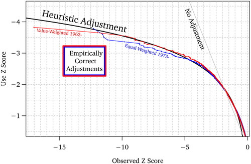
Figure 1 plots a visual illustration using two interesting example series. These are the value-weighted market rate of return from 1963 to 2023 and the equal-weighted market rate of return from 1973 to 2023. The plot shows the no-adjustment “naïve use” Z score input, which is useful if the data had come from a true normal distribution; the heuristic formula proposed Z score transform, $Z\prime ;$ and the empirically best Z-score. The plot reveals the following:

• For untransformed Z inputs between −0.2 and −1.9, the $Z\prime$ score after the heuristic-formula transform is less conservative (i.e., above the unadjusted Z score).⁴ However, (a) the differences between the untransformed Z and the transformed $Z\prime$ scores are small and (b) the heuristic $Z\prime$ scores happens to fit the empirical distribution of these market portfolio returns better than the unadjusted Z scores. It would thus have simply been the better score to use to assess the probability of negative returns in this domain.

• For untransformed Z scores more negative than −1.9, the adjusted $Z\prime$ score is both more conservative and progressively much better than the unadjusted Z score. For untransformed Z scores between −1.9 and −13, the heuristic formula $Z\prime$ fits the empirical distribution quite well per se. It is only for Z scores less than −13 that the heuristic formula fit deteriorates relative to the empirical distribution. Analysts may thus want to consider even more extreme adjustments than those proposed here. However, the rarity of such low return realizations, given only a century of stock returns, makes it is difficult also to judge how much trust one should place in the empirical distribution. This far in the tail, it may not be representative of the true distribution either.

Figure 1. Z Scores for Daily Market Rates of Return

Note. Explanations: The blue line is the Z score that best matches the empirical probability for the value-weighted market rate of return when using the normal distribution tables, beginning in 1962. It is the same case as that in Table 1. The red line is the same for the equal-weighted market rate of return, beginning in 1973. The thick black line is the quick-and-dirty adjustment-heuristic of $Z\prime =-1.25-\hspace{0.17em}\mathrm{\text{log}}\hspace{0.17em}(-Z).$ The diagonal straight line on the right is the unadjusted Z score. Interpretation: The heuristic formula can be recommended for all negative Z scores, even though it is less conservative between −0.2 and −1.9. (For these Z scores, the difference between the adjusted and unadjusted Z score is modest, and the adjusted Z’ fits the empirical return distribution better than Z.) For Z scores lower than, say, −13, an extra further adjustment could be wise—although such events are so rare, and thus difficult to assess in the empirical stock return distribution, that this may not even be the case.) Source: data/plotusethis.R: 2024/04/16 and CRSP.

Table 2 extends the analysis to other starting periods. The heuristic adjustment formula works just as well as it did from 1962 to 2023 in Table 1. The $Z\prime$ scores are again very close to what they should be given the empirical distribution. They are both empirically and visually difficult to differentiate.

Table 2. Daily Value-Weighted Market Rate of Return, Later Starts

Panel A: Post 1973/01/01, 12,861 days
Obsrvd		Empirical obsrvd		Bad inference		Corrected normal Z
RoR	Z	Emp CDF	Per Yr	Normal CDF	$\approx \mathrm{10\hspace{0.17em}}̂$	Optimal	Heuristic (Z′)
−0.1713	−16.08	0.00007774	50.8	0.00000000	−58	−3.78	−4.03
−0.0900	−8.46	0.00038871	10.2	0.00000000	−17	−3.36	−3.39
−0.0709	−6.68	0.00077742	5.1	0.00000000	−11	−3.16	−3.15
−0.0645	−6.07	0.00116614	3.4	0.00000000	−9	−3.04	−3.05
−0.0557	−5.25	0.00155485	2.5	0.00000007	−7	−2.96	−2.91
−0.0534	−5.04	0.00178807	2.2	0.00000023	−7	−2.91	−2.87
−0.0423	−4.00	0.00334292	1.2	0.00003119	−5	−2.71	−2.64
Panel B: Post 1998/01/01, 6,541 days
Obsrvd		Empirical obsrvd		Bad inference		Corrected normal Z
RoR	Z	Emp CDF	Per Yr	Normal CDF	$\approx \mathrm{10\hspace{0.17em}}̂$	Optimal	Heuristic (Z′)
−0.1201	−9.73	0.0001528	25.9	0.00000000	−22	−3.61	−3.53
−0.0829	−6.73	0.0007642	5.2	0.00000000	−11	−3.17	−3.16
−0.0662	−5.38	0.0015283	2.6	0.00000004	−7	−2.96	−2.93
−0.0589	−4.79	0.0022925	1.7	0.00000084	−6	−2.83	−2.82
−0.0507	−4.13	0.0030567	1.3	0.00001806	−5	−2.74	−2.67
−0.0493	−4.01	0.0036680	1.1	0.00002993	−5	−2.68	−2.64

Note. Explanations: See Table 1. Interpretation: For these two commonly used samples for the stock market statistical distribution, the heuristic fits well. Source: Data/empirical.R: 2024/04/16 and CRSP.

The appropriateness of the heuristic adjustment formula depends on the fat-tailedness of the distribution, which can be measured. Table 3 provides statistics for the kurtosis and maximum-likelihood degrees of freedom of the empirically observed distribution of rates of return for various market and two size (marketcap) portfolios. The two are not monotonically related, because the latter considers not just the kurtosis but also other moments in its fit. All empirical kurtoses are far above the 3.0 expected for the normal distribution. If Black Friday is excluded, the estimated degrees of freedom for Student T distributions lie between about 2.7 and 6; the exception is the small and equal-weighted market daily stock returns from 1973 on and the value-weighted market monthly stock returns from 1998 on, all of which reach above 7. The degree-of-freedom estimates for the data of Tables 1 and 2 were 3.05, 2.78, and 3.27, respectively. The heuristic formula fits well for all these cases.⁵

Table 3. Empirically Estimated Kurtosis and Student T Degrees of Freedom

			Empirically estimated
Frequency	Description	Sample	Kurtosis	df of T dist
Daily	Value-weighted stock market	–1962	19.2	2.09
		1962–	19.0	3.05	(Table 1)
		1973–	17.9	2.78	(Table 2A)
		1998–	12.0	3.27	(Table 2B)
	Log-value-weighted stock market	−1962	18.6	2.08
		1962–	21.6	3.03
		1973–	20.4	2.77
		1998–	12.3	3.32
	Equal-weighted stock market	–1962	26.8	1.91
		1962–	18.6	2.68
		1973–	18.6	7.41
		1998–	13.5	3.21
	Small decile	1973–	98.0	7.30	(Table 5A)
	Large decile		18.5	5.01	(Table 5B)
Monthly	Value-weighted stock market	–1962	10.8	2.89
		1962–	4.8	6.25
		1973–	4.9	6.11
		1998–	4.1	7.03	(Table 4)
	Log-value-weighted stock market	−1962	9.5	2.76
		1962–	5.6	5.59
		1973–	5.7	5.44
		1998–	4.6	5.74
	Equal-weighted stock market	–1962	16.5	2.28
		1962–	5.8	4.75
		1973–	6.2	4.48
		1998–	5.0	4.66
	Small decile	1973–	9.7	3.16
	Large decile		4.7	6.24

Note. Explanations: The empirical kurtosis for daily returns ranges from a low of 12 to a high of 100. For monthly returns, it ranges from a low of 4 to a high of 17. The empirically best-fitting T distributions have degrees of freedom ranging from 1.91 to 7.41. The two do not necessarily align, because the best fitting T distribution is also fit to higher moments, not just the kurtosis. Moreover, if the true degrees of freedom were as estimated, the true kurtosis would be infinite for all degrees of freedom less than 4.0. Interpretation: The overall stock market and even extreme size deciles have distributions that are similarly fat-tailed, regardless of how and when they are measured. Thus, the heuristic is likely to fit well. Source: data/empirical.R: 2024/04/16 (grep for ’Best df_T is’) and CRSP.

To assess the robustness of the adjustment formula, we can look briefly at one more extreme case in which the estimate for the degrees of freedom is higher (less kurtotic, more Gaussian normal) and in which there are far fewer observations. Table 4 examines value-weighted monthly market rates of return after 1978, with its estimate for the Student T degrees of freedom of 7.03. There are only 312 months to work with. Table 4 shows that its worst month had a rate of return equivalent to a Z score of −4.08. With 312 months, the empirical frequency suggests a monthly occurrence of about 0.3%, that is, about once every 26 years. The appropriate Z score to match the empirical distribution in a normal table would have been −2.73. The heuristic formula adjusts the more misleading $Z=-4.08$ score to a better $Z\prime =-2.77$ score.

Table 4. Monthly Value-Weighted Market Rate of Return, 1998, 312 Months

Obsrvd		Empirical obsrvd		Bad inference		Corrected normal Z
RoR	Z	Emp CDF	Per Yr	Normal CDF	$\approx \mathrm{10\hspace{0.17em}}̂$	Optimal	Heuristic (Z′)
−0.1849	−4.08	0.003185	26.2	0.00002229	−5	−2.73	−2.66
−0.1011	−2.31	0.015924	5.2	0.01056976	−2	−2.15	−2.09

Note. Explanations: See Table 1. These data are monthly and begin on 1998/01/01. Interpretation: Even for the distribution of monthly rates of return, with their higher estimated numbers of degrees of freedom (i.e., more resemblance to a Gaussian normal distribution than the dailies), the heuristic fits well. Source: Data/empirical.R: 2024/04/16 and CRSP.

In general, the formula seems to fit remarkably well for Student T distributions from about 2 to about 10 degrees of freedom. Beyond 10 degrees of freedom, the Student T distribution becomes more like the normal distribution and the use of the unadjusted Z rather than the adjusted $Z\prime$ becomes more attractive again. However, stock returns are rarely this normal.

Table 5 expands the perspective to non-market portfolios. In particular, it explores the two extreme decile marketcap portfolios on CRSP. There is not much to be said. The formula does a good job adjusting poor Z scores to better $Z\prime$ scores for both portfolios. Recall that Table 3 showed the degrees of freedom estimates for these portfolios in this sample to be about 5 and 7.

Table 5. Extreme CRSP Size Decile Rates of Return, Post 1973, 12,861 Days

Panel A: 01 Smallest capitalization decile
Obsrvd		Empirical obsrvd		Bad inference		Corrected normal Z (Z′)
RoR	Z	Emp CDF	Per Yr	Normal CDF	$\approx \mathrm{10\hspace{0.17em}}̂$	Optimal	Heuristic
−0.1375	−14.37	0.00007774	50.8	0.00000000	−46	−3.78	−3.91
−0.0805	−8.44	0.00038871	10.2	0.00000000	−17	−3.36	−3.38
−0.0687	−7.21	0.00077742	5.1	0.00000000	−13	−3.16	−3.22
−0.0561	−5.90	0.00116614	3.4	0.00000000	−9	−3.04	−3.02
−0.0485	−5.11	0.00155485	2.5	0.00000016	−7	−2.96	−2.88
−0.0476	−5.01	0.00171033	2.3	0.00000027	−7	−2.93	−2.86
−0.0378	−3.99	0.00357615	1.1	0.00003254	−4	−2.69	−2.63
Panel B: 10 largest capitalization decile
Obsrvd		Empirical obsrvd		Bad inference		Corrected normal Z
RoR	Z	Emp CDF	Per Yr	Normal CDF	$\approx \mathrm{10\hspace{0.17em}}̂$	Optimal	Heuristic (Z′)
−0.1828	−16.84	0.00007774	50.8	0.00000000	−63	−3.78	−4.07
−0.0879	−8.12	0.00038871	10.2	0.00000000	−16	−3.36	−3.34
−0.0709	−6.56	0.00077742	5.1	0.00000000	−11	−3.16	−3.13
−0.0630	−5.83	0.00116614	3.4	0.00000000	−9	−3.04	−3.01
−0.0571	−5.28	0.00155485	2.5	0.00000006	−7	−2.96	−2.91
−0.0540	−5.00	0.00163259	2.4	0.00000029	−7	−2.94	−2.86
−0.0429	−3.98	0.00318744	1.2	0.00003423	−4	−2.73	−2.63

Note. Explanations: See Table 1. These data begin on 1973/01/01. Interpretation: Even for the daily distributions of portfolios with small and big firms, the heuristic fits well. Source: Data/empirical.R: 2024/04/16 and CRSP.

Table 6 expands the perspective even further, now to the zero-investment factors developed by Fama and French (2015) (and some others posted on Ken French’s website). Again, the heuristic $Z\prime$ estimates fit just as well as they did for the overall market, not only in the United States but also in Europe and Japan.

Table 6. Fama–French Daily Factors, Post 1973

		Empirically estimated
Region	Factor	Kurtosis	df of T dist
USA	SMB	19.3	4.60
	HML	12.9	2.47
	RMW	11.3	2.70
	CMA	12.4	3.28
	MOM	21.1	2.20
	REV	9.5	3.07
	STREV	33.6	2.12
EUR	SMB	9.6	3.32
	HML	9.9	2.65
	RMW	11.5	4.16
	CMA	8.2	2.90
JPN	SMB	11.1	3.80
	HML	7.9	2.67
	RMW	10.2	3.45
	CMA	9.6	2.90

Note. Explanations: See Table 3. Factors are as named by Ken French. Interpretation: The factor portfolios have distributions that are similarly fat-tailed, regardless of how and when they are measured. The heuristic would thus fit well. Source: Data/empirical.R: 2024/04/16 and Ken French’s website.

Table 7 expands the perspective further again, this time to (thousands of) individual US stocks. And, again, the Z′ performance seem as good as before. The adjustment formula would work quite well for at least about 95% of individual stocks.

An earlier draft explored whether kurtosis also distorts regression coefficients and consequent inference, for example, in Fama–Macbeth regressions that explore whether value metrics can predict future stock returns. The answer is that such coefficient inference is barely distorted at all. Ordinary least squares coefficients and coefficient standard errors are very robust to non-normal conditional error distributions. (This extends to even more extremely different distributions, like the binomial distribution.) Note, however, that if such regressions are then used to predict stock return performance and losses, not only the coefficient estimates but also the error estimates become relevant again. In this case, the above empirical heuristic adjustment would become important again.

Table 7. Individual Stocks

	Empirically estimated
	Kurtosis	df of T
Mean	49.1	3.96
Sd	192.2	19.28
Smallest	3.1	0.48
1%	5.6	1.12
5%	7.3	1.51
25%	11.4	2.21
Median	16.9	2.67
75%	32.2	3.22
95%	140.0	4.74
99%	624.7	8.32
Biggest	8,509.x	859.8x
N = 10,585 Stocks

Note. Explanations: See Table 3. Estimated statistics are as in earlier tables, but here they are for individual stocks with at least 2,500 rates of returns from 1973/01/01. Interpretation: There are about 5% of stocks for which even the heuristic would have underestimated the left tail (though far less so than the unadjusted Z score), and there are fewer than 1% of stocks for which the heuristic would have been worse than the assumption of a plain normal distribution. Source: Data/fattailed-individual-stocks.R: 2024/04/16 and CRSP.

Conclusion

There is only one important aspect of this paper worth remembering:

• For negative Z scores, better probability assessments for stock and portfolio returns can be obtained by using the heuristic adjustment formula: $$Z\prime =-1.25-\hspace{0.17em}\mathrm{\text{log}}\hspace{0.17em}(-Z).$$

The improvement is modest for Z scores between 0 and −2, but it becomes progressively larger and more important for Z scores more negative than −2, that is, further in the left tail.

Secondarily, this paper also offered some empirical evidence about the fat-tailedness of a variety of recent stock and portfolio return distributions. If one wants to think of daily or monthly stock returns in the context of Student T distributions, empirical stock returns have resembled Student T distributions with between 2 and 7 degrees of freedom when including Black Tuesday (October 1929) and between 3 and 7 degrees of freedom when sample periods start thereafter.

Disclosure:

This research was conducted independently, without external support or conflicts of interest.

Additional information

Notes on contributors

Ivo Welch

Ivo Welch is the J. Fred Weston Distinguished Professor at the Anderson Graduate School of Management at UCLA, Los Angeles, CA.

Notes

1 Even when the data are available (which is not always the case), it is also easy to make a mistake working with the unadjusted standard deviation and the Student T distribution. Jonathan Lewellen graciously pointed out to me that my first draft had missed a $\sqrt{d{f}_T/(d{f}_T-2)}$ necessary correction.

2 A common way to diagnose (but not adjust for) this problem statistically is through maximum likelihood estimate of the power coefficient in the Pareto distribution of extreme values (Hill 1975). (This is the slope of the extreme value distribution at the tail beyond a researcher-chosen cutoff.) Not surprisingly, the Hill statistics strongly indicate that returns are not drawn from a normal distribution.

3 The illustrative Z scores in the table were chosen as the 5th, 10th, 15th, and 20th lowest realization plus, where appropriate, the realizations closest to Z scores of −6, −5, and −4.

4 There are two roots to $-1.25-\hspace{0.17em}\mathrm{\text{log}}\hspace{0.17em}(-Z)=Z.$ Due to the local curvature of the log function, the difference between the unadjusted Z and the adjusted $Z\prime$ score remains small, between 0 and −2.

5 I am not using a formal metric to judge “fitting well.” There are issues related to whether a difference from 1.1 to 1.4 is more important than a difference from 4.1 to 4.4. The probabilities are 0.136, 0.080, 0.001, and 0.0003, respectively. The first two have higher absolute probability differences (0.055 vs. 0.0006), while the latter two have higher relative probability differences (1.7 vs. 2.9 times).

Appendix A.

Chosen Formula Approximation

A good adjustment formula translates the Z statistic of the empirical distribution into an equivalent “as-if” Z statistic of a normal distribution. Ideally, an adjustment-map function $g(x )$ would satisfy, for all x (or at least for very negative x) that the resulting left-tail probabilities match: $$F(x)=F_N(g(x))\mathrm{\hspace{1em}}\hspace{1em}\iff \mathrm{\hspace{1em}}\hspace{1em}g(x)=Q_N(F(x)),$$ where F is the to-be-matched cumulative distribution function and Q is the quantile function (the inverse of F). Although this is easy to approximate numerically, there are no closed-form solutions for g even when the to-be-matched distribution is not an empirical but a well-known analytical statistical distribution (such as a Student T). Moreover, we are also not interested in a perfect adjustment formula $g(·)$ but in an approximate and more easily remembered heuristic one. The log-linear form, that is, $\widehat{g}(x)=a+b·\hspace{0.17em}\mathrm{\text{log}}\hspace{0.17em}(|x|),$ with its strong curvature in x, is indicated by a visual inspection of the empirical distribution in Figure 1. Similar log-related formulas appear commonly in extreme-value statistics.

For intuition, consider the case in which the true distribution, $F(z),$ is the (more fat-tailed) Student T distribution. Table A1 shows the best coefficients on an adjustment formula of the form $a+b·\hspace{0.17em}\mathrm{\text{log}}\hspace{0.17em}(-Z)$ for Student T distributions with various degrees of freedom (fat-tailedness). The chosen heuristic approximation of $-1.25-\hspace{0.17em}\mathrm{\text{log}}\hspace{0.17em}(-Z)$ is near a best-fit 3.2 degrees of freedom, rounded to make the formula easier to remember. Although the (a,b) coefficients look different for different degrees of freedom, they move in opposite directions and thus their fitted values are not greatly different. For example, for an empirical Z score of −5, for 2 degrees of freedom (i.e., the −2.07,−0.57 coefficients) suggests a revised Z score of −2.99. For 3 degrees of freedom, the Z score is −2.95. For 4 degrees of freedom, it is −3.06. The rounded in-text heuristic of $Z\prime =-1.25-1·\hspace{0.17em}\mathrm{\text{log}}\hspace{0.17em}(-Z)$ suggests −2.86. Compared to the unadjusted Z of −5, the disagreements among approximation formulas ranging from −2.86 to −3.06 appear trivial.

Table A1. Well-Fitting Formula on Z Scores Below −3

Used	dfT	Kurtosis		a	b	Heuristic is more conservative below Z of
		Simul	(Theory)
37,381	2.0		(∞)	−2.07	−0.57	−2.62
49,997	2.2		(∞)	−1.90	−0.64	−2.47
59,266	2.4		(∞)	−1.77	−0.70	−2.37
65,178	2.6		(∞)	−1.66	−0.76	−2.30
68,497	2.8		(∞)	−1.58	−0.82	−2.25
70,013	3.0		(∞)	−1.51	−0.88	−2.21
70,332	3.2		(∞)	−1.46	−0.93	−2.18
69,877	3.4		(∞)	−1.40	−0.98	−2.15
68,933	3.6		(∞)	−1.35	−1.02	−2.13
67,688	3.8		(∞)	−1.31	−1.07	−2.11
66,267	4.0		(∞)	−1.27	−1.11	−2.09
58,648	5.0	8.2	(9.0)	−1.09	−1.31	−1.99
52,018	6.0	5.9	(6.0)	−0.94	−1.48	−1.86
46,746	7.0	5.0	(5.0)	−0.81	−1.63
36,574	10.0	4.0	(4.0)	−0.53	−1.96
15,542	100.0	3.1	(3.1)	0.61	−3.23
13,699	1000.0	3.0	(3.0)	0.80	−3.44
	Recommended Heuristic:			−1.25	−1.00	−1.88

Note. Explanations: Based on a simulated perfect interval grid of 10 million draws from a Student T distribution with the degrees of freedom as described in the second column, this table shows the coefficients on the appropriate inference from a raw Z score to the best-as-if-Gaussian-normal Z score in the formula $Z\prime =a+b·\hspace{0.17em}\mathrm{\text{log}}\hspace{0.17em}(-Z ),$ fitting only drawn values with scaled values (Z scores) of less than −3 (the number of which is indicated in the first column). (The parenthetical value in the kurtosis is the theoretically correct one [$3+6/({\text{df}}_T-4)$ for ${\text{df}}_T>4$].). Interpretation: The adjustment-heuristic formula of $-1.25-\hspace{0.17em}\mathrm{\text{log}}\hspace{0.17em}(-Z )$ used in the paper is geared roughly toward a Student T distribution with 3 to 3.5 degrees of freedom. It is more conservative for Z values less than −1.88. (Note: There are actually two roots. The second root, in the latter case, is about −0.2, visible also in Figure 1. With lesser kurtosis, the $g(·)$ no longer intersects at all.). Source: Data/find-good-formula.R: 2024/04/16, 2024/06/19. No data.

Natural heterogeneity among different empirical return series and general robustness considerations suggest that this heuristic formula is often “good enough.” Researchers who need more accuracy are advised to work with estimates of kurtosis and/or their distributions directly rather than rely on the simple approximation used here. However, it is unclear whether such accuracy can even be meaningfully empirically obtained, given the limited number of centuries of stock return data available.

References

- Bollerslev, Tim. 1986. “Generalized Autoregressive Conditional Heteroskedasticity.” Journal of Econometrics 31 (3): 307–327. doi:10.1016/0304-4076(86)90063-1.
- Fama, Eugene F. 1965. “The Behavior of Stock-Market Prices.” The Journal of Business 38 (1): 34–105. doi:10.1086/294743.
- Fama, Eugene F., and Kenneth R. French. 2015. “A Five-Factor Asset Pricing Model.” Journal of Financial Economics 116 (1): 1–22. doi:10.1016/j.jfineco.2014.10.010.
- Hill, Bruce M. 1975. “A Simple General Approach to Inference about the Tail of a Distribution.” The Annals of Statistics 3 (5): 1163–1174. doi:10.1214/aos/1176343247.
- Kon, Stanley J. 1984. “Models of Stock Returns—A Comparison.” The Journal of Finance 39 (1): 147–165. doi:10.2307/2327673.
- Koning, Nico, Daniel T. Cassidy, and Rachid Ouyed. 2018. “Extended Model of Stock Price Behaviour.” Journal of Mathematical Finance 08 (01): 1–13. doi:10.4236/jmf.2018.81001.
- Mandelbrot, Benoit B., and Benoit B. Mandelbrot. 1997. The Variation of Certain Speculative Prices. The University of Chicago Press.
- Taleb, Nassim Nicholas. 2007. The Black Swan: The Impact of the Highly Improbable. (2nd ed) New York: Random House.
- Welch, Ivo. 2016. “The (Time-Varying) Importance of Disaster Risk.” Financial Analysts Journal 72 (5): 14–30. doi:10.2469/faj.v72.n5.3.