The COS method for option valuation under the SABR dynamics

ABSTRACT

In this paper, we consider the COS method for pricing European and Bermudan options under the stochastic alpha beta rho (SABR) model. In the COS pricing method, we make use of the characteristic function of the discrete forward process. We observe second-order convergence by using a second-order Taylor scheme in the discretization, or by using Richardson extrapolation in combination with a Euler–Maruyama discretization on the forward process. We also consider backward stochastic differential equations under the SABR model, using the discretized forward process and Fourier-cosine expansion for the occurring expectations. For this purpose, we extend the so-called BCOS method from one to two dimensions.

Keywords:

• COS method
• Euler–Maruyama scheme
• backward stochastic differential equation
• SABR
• Richardson extrapolation

2010 AMS Subject Classifications:

• 60E10
• 65C30
• 91G60

1. Introduction

Efficient valuation of financial options is an important issue in financial mathematics. In the last few decades, many pricing methods have been introduced, for example, convenient formulas [3,17,19], Monte Carlo methods [5,15,20], finite difference methods [10,18,22], quadrature methods [7] and also Fourier methods [6,12,25,26,28,33]. A variety of option pricing methods is compared in [37], including several Fourier methods. This type of methods, such as the COS method [12,33], is based on the characteristic function (ChF) of the underlying process to determine the option value. However, often no analytic expression for the ChF of the underlying process is available. The authors in [35] use the ChF of the discrete process to price options and to solve backward stochastic differential equations (BSDEs). We extend this so-called BCOS method (BSDE COS method) from one to two dimensions, see also [36], in order to solve BSDEs under the so-called stochastic alpha beta rho (SABR) SDE system. The BCOS method approximates the solutions of BSDEs by iterating backwards in time, so we do not need to simulate the forward process. The theory of BSDEs is described in detail in the literature [4,11,29,30] and relevant applications in mathematical finance are studied in for example [23,34,38]. In this paper, we pay attention especially to the valuation of options with the BCOS method. The basis is formed by using the COS method under SABR dynamics, and we will also explain this. As we will observe, the BCOS method may suffer from the curse of dimensionality, as well as quadrature methods and finite difference methods. Nevertheless, these methods are widely used for two-dimensional models. Therefore, investigation of the two-dimensional BCOS method is of value to acquire a wider diversity in methods.

To obtain rapid convergence, we will employ Richardson extrapolation in combination with the Euler–Maruyama SDE discretization (see also [21]). In particular, we price European and Bermudan options under a two-dimensional model, like the SABR model [17]. Due to the closed-form expression of the implied volatility, the Hagan formula [17], the SABR model is a widely used stochastic local volatility model in the financial world. Many pricing methods for SABR-like models have been presented in the literature, like [2,9,16,18,27], however, many of those methods are mainly accurate for valuing European options with short maturities under the SABR model. In [1] a pricing method is given, which is accurate for options with long maturities, but this method is not applicable for all parameter sets [1]. When we work on the risk neutral measure, we can simply use the COS method, for European and Bermudan options. Under the real-world measure, we encounter a BSDE, where the terminal condition is given by the payoff function.

This paper is organized as follows. In Section 2, we introduce the two-dimensional COS method for pricing European and Bermudan options. We discuss the two-dimensional BCOS method in Section 3. Furthermore, we present several numerical experiments in Section 4. Finally, we conclude in Section 5.

2. The two-dimensional COS method

In this section, we explain the two-dimensional COS method for pricing European and Bermudan options. We assume that the underlying forward stochastic differential equations (FSDEs) can be written in the following general form: (1) $\begin{array}{rl}\mathrm{d}{X}_t^1& ={\mu }_1(X_t^1,X_t^2)\mathrm{d}t+{\sigma }_1(X_t^1,X_t^2)\mathrm{d}{W}_t^1,\\ \mathrm{d}{X}_t^2& ={\mu }_2(X_t^1,X_t^2)\mathrm{d}t+\rho {\sigma }_2(X_t^1,X_t^2)\mathrm{d}{W}_t^1+\sqrt{1-{\rho }^2}{\sigma }_2(X_t^1,X_t^2)\mathrm{d}{W}_t^2,\end{array}$(1) where $t\ge 0$, $X_0^1=x_1$, $X_0^2=x_2$, the correlation $\rho \in (-1,1)$, and $W_t^1$ and $W_t^2$ are independent standard Brownian motions on a filtered probability space $\mathcal{F}$. The functions ${\sigma }_1,{\sigma }_2,{\mu }_1,{\mu }_2:{\mathbb{R}}^2\to \mathbb{R}$ are assumed to be twice differentiable with respect to $x_1$ and $x_2$. When the corresponding bivariate ChF cannot easily be derived, it is possible to approximate it by the bivariate ChF of the discretized FSDE process. For this discretization, we use the Euler–Maruyama scheme and also the 2.0-weak-Taylor scheme.

We are interested in pricing options under the SABR model [17]. The FSDEs of the SABR model are of the same form as Formula (1(1) $\begin{array}{rl}\mathrm{d}{X}_t^1& ={\mu }_1(X_t^1,X_t^2)\mathrm{d}t+{\sigma }_1(X_t^1,X_t^2)\mathrm{d}{W}_t^1,\\ \mathrm{d}{X}_t^2& ={\mu }_2(X_t^1,X_t^2)\mathrm{d}t+\rho {\sigma }_2(X_t^1,X_t^2)\mathrm{d}{W}_t^1+\sqrt{1-{\rho }^2}{\sigma }_2(X_t^1,X_t^2)\mathrm{d}{W}_t^2,\end{array}$(1) ), that is, (2) $\begin{array}{rl}\mathrm{d}{F}_t& ={\alpha }_t(F_t{)}^{\beta }\mathrm{d}{W}_t^1,F_0=f,\\ \mathrm{d}{\alpha }_t& =\rho \nu {\alpha }_t\mathrm{d}{W}_t^1+\sqrt{1-{\rho }^2}\nu {\alpha }_t\mathrm{d}{W}_t^2,{\alpha }_0=\alpha ,\end{array}$(2) where $F_t$ is the forward, for example, the forward swap rate, and ${\alpha }_t$ denotes the volatility. Furthermore, $W^1$ and $W^2$ are independent standard Brownian motions under the forward measure, exponent $0\le \beta \le 1$, the volatility of the volatility $\nu \ge 0$ and the initial forward f and volatility α are non-negative. The authors in [17] proposed a very convenient formula to calculate the Black implied volatility under the SABR model. This formula, also known as the Hagan formula, may however sometimes lead to arbitrage possibilities for low strikes, as one can observe by examining the corresponding PDF [36]. The Hagan formula is not accurate for pricing options with long maturities [1,18,36].

As no analytic expression for the bivariate ChF of the SABR model is available, it may be difficult to calculate accurate reference values for our purposes. That is why we also consider the Heston model¹ as a reference model for convergence purposes. The ChF of the Heston model is known, which ensures the availability of accurate reference prices for European and Bermudan options. The FSDEs can be written in the form of Formula (1(1) $\begin{array}{rl}\mathrm{d}{X}_t^1& ={\mu }_1(X_t^1,X_t^2)\mathrm{d}t+{\sigma }_1(X_t^1,X_t^2)\mathrm{d}{W}_t^1,\\ \mathrm{d}{X}_t^2& ={\mu }_2(X_t^1,X_t^2)\mathrm{d}t+\rho {\sigma }_2(X_t^1,X_t^2)\mathrm{d}{W}_t^1+\sqrt{1-{\rho }^2}{\sigma }_2(X_t^1,X_t^2)\mathrm{d}{W}_t^2,\end{array}$(1) ), that is, (3) $\begin{array}{rl}\mathrm{d}{X}_t& =-\frac{1}{2}{A}_t\mathrm{d}t+\sqrt{A_t}\mathrm{d}{W}_t^1,X_0=x,\\ \mathrm{d}{A}_t& =\rho \nu \sqrt{A_t}\mathrm{d}{W}_t^1+\sqrt{1-{\rho }^2}\nu \sqrt{A_t}\mathrm{d}{W}_t^2,A_0=a,\end{array}$(3) where $X_t$ denotes the log-asset process and $A_t$ is the variance. Furthermore, $W^1$ and $W^2$ are independent standard Brownian motions, the volatility of the volatility parameter ν and the initial variance a are both non-negative. FSDEs (3(3) $\begin{array}{rl}\mathrm{d}{X}_t& =-\frac{1}{2}{A}_t\mathrm{d}t+\sqrt{A_t}\mathrm{d}{W}_t^1,X_0=x,\\ \mathrm{d}{A}_t& =\rho \nu \sqrt{A_t}\mathrm{d}{W}_t^1+\sqrt{1-{\rho }^2}\nu \sqrt{A_t}\mathrm{d}{W}_t^2,A_0=a,\end{array}$(3) ) do not obey the Feller condition, so we have to make sure that we choose the computational domain, see Appendix 2, such that the variance process can attain any non-negative value. The Heston model (3(3) $\begin{array}{rl}\mathrm{d}{X}_t& =-\frac{1}{2}{A}_t\mathrm{d}t+\sqrt{A_t}\mathrm{d}{W}_t^1,X_0=x,\\ \mathrm{d}{A}_t& =\rho \nu \sqrt{A_t}\mathrm{d}{W}_t^1+\sqrt{1-{\rho }^2}\nu \sqrt{A_t}\mathrm{d}{W}_t^2,A_0=a,\end{array}$(3) ) is an affine model, so an analytic formula for its bivariate ChF is known [36]: (4) $\begin{array}{rl}& {\phi }_{(X_{t+\mathrm{\Delta }t},A_{t+\mathrm{\Delta }t})}(u_1,u_2|X_t,A_t)\\ & =\exp \left(\mathrm{i}{u}_1{X}_t+\frac{1}{{\nu }^2}\left[\zeta \tan \left(\arctan \left[\frac{\mathrm{i}{u}_2{\nu }^2+\mathrm{i}{u}_1\rho \nu }{\zeta }\right]+\frac{\mathrm{\Delta }t}{2}\zeta \right)-\mathrm{i}{u}_1\rho \nu \right]A_t\right),\end{array}$(4) where (5) $\zeta =\sqrt{-\mathrm{i}{u}_1{\nu }^2+u_1^2({\rho }^2-1){\nu }^2}.$(5)

In Section 2.1, we give the Taylor schemes and the necessary formulas to price European options with the COS method. Also, we detail the procedure for valuing Bermudan options in this section. We provide an approach to price multiple European options under the SABR model in one computation in Section 2.2. We describe the use of Richardson extrapolation in Section 2.3. The computational complexity of the proposed method is discussed in Section 2.4.

2.1. Pricing options with the COS method

Just as in [36], we define a time-grid $t_m=m\mathrm{\Delta }t$ for $m=0,1,\dots ,M$, with fixed time steps $\mathrm{\Delta }t=T/M$. We write ${\mathbf{\text{X}}}_m={\mathbf{\text{X}}}_{t_m}$, $X_m^j=X_{t_m}^j$, j=1,2. The discrete forward process is denoted by ${\mathbf{\text{X}}}_m^{\mathrm{\Delta }}={\mathbf{\text{X}}}_{t_m}^{\mathrm{\Delta }}$ and $X_m^{j,\mathrm{\Delta }}=X_{t_m}^{j,\mathrm{\Delta }}$. To determine the values of $X_{m+1}^{j,\mathrm{\Delta }}$, $m=0,\dots ,M-1$, and given ${\mathbf{\text{X}}}_m=\mathbf{\text{x}}=(x_1,x_2)$, we use the Euler–Maruyama and the 2.0-weak-Taylor schemes. We write the discrete schemes for Formula (1(1) $\begin{array}{rl}\mathrm{d}{X}_t^1& ={\mu }_1(X_t^1,X_t^2)\mathrm{d}t+{\sigma }_1(X_t^1,X_t^2)\mathrm{d}{W}_t^1,\\ \mathrm{d}{X}_t^2& ={\mu }_2(X_t^1,X_t^2)\mathrm{d}t+\rho {\sigma }_2(X_t^1,X_t^2)\mathrm{d}{W}_t^1+\sqrt{1-{\rho }^2}{\sigma }_2(X_t^1,X_t^2)\mathrm{d}{W}_t^2,\end{array}$(1) ) in general form, as follows: (6) $\begin{array}{rl}{X}_{m+1}^{j,\mathrm{\Delta }}& =x_j+m_j\left(\mathbf{\text{x}}\right)\mathrm{\Delta }t+s_j^1\left(\mathbf{\text{x}}\right)\mathrm{\Delta }{W}_{m+1}^1+s_j^2\left(\mathbf{\text{x}}\right)\mathrm{\Delta }{W}_{m+1}^2+{\kappa }_j^{1,2}\left(\mathbf{\text{x}}\right)\mathrm{\Delta }{W}_{m+1}^1\mathrm{\Delta }{W}_{m+1}^2\\ & +{\kappa }_j^1\left(\mathbf{\text{x}}\right)(\mathrm{\Delta }{W}_{m+1}^1{)}^2+{\kappa }_j^2(\mathbf{\text{x}}\left)\right(\mathrm{\Delta }{W}_{m+1}^2{)}^2+{\psi }_j\left(\mathbf{\text{x}}\right){\mathrm{\Psi }}_{m+1},\end{array}$(6) where $\mathrm{\Delta }{W}_{m+1}^1$ and $\mathrm{\Delta }{W}_{m+1}^2$ are uncorrelated and normally distributed Wiener increments with mean zero and variance $\mathrm{\Delta }t$, and ${\mathrm{\Psi }}_{m+1}$ is an independent random variable with probability $P({\mathrm{\Psi }}_{m+1}=\pm \mathrm{\Delta }t)=\frac{1}{2}$.

For the Euler–Maruyama scheme,² we have (7) $\begin{array}{rl}{m}_1\left(\mathbf{\text{x}}\right)& ={\mu }_1\left(\mathbf{\text{x}}\right),s_1^1\left(\mathbf{\text{x}}\right)={\sigma }_1\left(\mathbf{\text{x}}\right),s_1^2\left(\mathbf{\text{x}}\right)=0,{\kappa }_1^{1,2}\left(\mathbf{\text{x}}\right)=0,\\ {\kappa }_1^1\left(\mathbf{\text{x}}\right)& =0,{\kappa }_1^2\left(\mathbf{\text{x}}\right)=0,{\psi }_1\left(\mathbf{\text{x}}\right)=0,\\ m_2\left(\mathbf{\text{x}}\right)& ={\mu }_2\left(\mathbf{\text{x}}\right),s_2^1\left(\mathbf{\text{x}}\right)=\rho {\sigma }_2\left(\mathbf{\text{x}}\right),s_2^2\left(\mathbf{\text{x}}\right)=\sqrt{1-{\rho }^2}{\sigma }_2\left(\mathbf{\text{x}}\right),{\kappa }_2^{1,2}\left(\mathbf{\text{x}}\right)=0,\\ {\kappa }_2^1\left(\mathbf{\text{x}}\right)& =0,{\kappa }_2^2\left(\mathbf{\text{x}}\right)=0,{\psi }_2\left(\mathbf{\text{x}}\right)=0.\end{array}$(7)

The functions associated with the 2.0-weak-Taylor scheme are given in Appendix 1.

According to [24], the definitions of the order of strong convergence and the order of weak convergence are:

Definition 2.1.

The discrete process $X^{\mathrm{\Delta }}$ converges in the strong sense with order ${\gamma }_1\in (0,\mathrm{\infty }]$ if there exists a finite constant C and a positive constant δ such that (8) $\mathbb{E}[|X_M-X_M^{\mathrm{\Delta }}|]\le C(\mathrm{\Delta }t{)}^{{\gamma }_1},$(8) for any time discretization with maximum step size $\mathrm{\Delta }t\in (0,\delta )$.

Definition 2.2.

Discrete process $X^{\mathrm{\Delta }}$ converges in the weak sense with order ${\gamma }_2\in (0,\mathrm{\infty }]$ if for any polynomial h there exists a finite constant C and a positive constant δ such that (9) $|\mathbb{E}\left[h\right(X_M\left)\right]-\mathbb{E}\left[h\right(X_M^{\mathrm{\Delta }}\left)\right]|\le C(\mathrm{\Delta }t{)}^{{\gamma }_2},$(9) for any time discretization with maximum step size $\mathrm{\Delta }t\in (0,\delta )$.

For the Euler scheme, the order of strong convergence is ${\gamma }_1=0.5$ and the order of weak convergence is ${\gamma }_2=1$, while for the 2.0-weak-Taylor scheme ${\gamma }_2=1$ and ${\gamma }_1\ge 0.5$. The strong order of convergence of the 2.0-weak-Taylor scheme equals 1 when Equation (1(1) $\begin{array}{rl}\mathrm{d}{X}_t^1& ={\mu }_1(X_t^1,X_t^2)\mathrm{d}t+{\sigma }_1(X_t^1,X_t^2)\mathrm{d}{W}_t^1,\\ \mathrm{d}{X}_t^2& ={\mu }_2(X_t^1,X_t^2)\mathrm{d}t+\rho {\sigma }_2(X_t^1,X_t^2)\mathrm{d}{W}_t^1+\sqrt{1-{\rho }^2}{\sigma }_2(X_t^1,X_t^2)\mathrm{d}{W}_t^2,\end{array}$(1) ) satisfies the following commutativity conditions [24]: (10) $\sqrt{1-{\rho }^2}{\sigma }_2\left(\mathbf{\text{x}}\right)\frac{\mathrm{\partial }{\sigma }_1\left(\mathbf{\text{x}}\right)}{\mathrm{\partial }{x}_2}=0\mathrm{and}\sqrt{1-{\rho }^2}{\sigma }_1\left(\mathbf{\text{x}}\right)\frac{\mathrm{\partial }{\sigma }_2\left(\mathbf{\text{x}}\right)}{\mathrm{\partial }{x}_1}=0\mathrm{\forall }{x}_1,x_2\in {\mathbb{R}}^2.$(10)

As observed in [36], the convergence of the COS method for pricing European options only depends on the order of weak convergence of the discretization scheme, and not on its order of strong convergence, because European options are not path-dependent. In Example 4.2 we observe that even for Bermudan options the order of weak convergence is leading for the rate of convergence. That is why we can use a weak-Taylor scheme for the discretization. Also, this implies that for application of the COS method it does not matter whether the FSDEs in Equation (1(1) $\begin{array}{rl}\mathrm{d}{X}_t^1& ={\mu }_1(X_t^1,X_t^2)\mathrm{d}t+{\sigma }_1(X_t^1,X_t^2)\mathrm{d}{W}_t^1,\\ \mathrm{d}{X}_t^2& ={\mu }_2(X_t^1,X_t^2)\mathrm{d}t+\rho {\sigma }_2(X_t^1,X_t^2)\mathrm{d}{W}_t^1+\sqrt{1-{\rho }^2}{\sigma }_2(X_t^1,X_t^2)\mathrm{d}{W}_t^2,\end{array}$(1) ) satisfy the commutativity condition (10(10) $\sqrt{1-{\rho }^2}{\sigma }_2\left(\mathbf{\text{x}}\right)\frac{\mathrm{\partial }{\sigma }_1\left(\mathbf{\text{x}}\right)}{\mathrm{\partial }{x}_2}=0\mathrm{and}\sqrt{1-{\rho }^2}{\sigma }_1\left(\mathbf{\text{x}}\right)\frac{\mathrm{\partial }{\sigma }_2\left(\mathbf{\text{x}}\right)}{\mathrm{\partial }{x}_1}=0\mathrm{\forall }{x}_1,x_2\in {\mathbb{R}}^2.$(10) ) or not.

Theorem 2.1.

The analytic expression for the bivariate ChF of ${\mathbf{\text{X}}}_{m+1}^{\mathrm{\Delta }},$ as in Equation (6(6) $\begin{array}{rl}{X}_{m+1}^{j,\mathrm{\Delta }}& =x_j+m_j\left(\mathbf{\text{x}}\right)\mathrm{\Delta }t+s_j^1\left(\mathbf{\text{x}}\right)\mathrm{\Delta }{W}_{m+1}^1+s_j^2\left(\mathbf{\text{x}}\right)\mathrm{\Delta }{W}_{m+1}^2+{\kappa }_j^{1,2}\left(\mathbf{\text{x}}\right)\mathrm{\Delta }{W}_{m+1}^1\mathrm{\Delta }{W}_{m+1}^2\\ & +{\kappa }_j^1\left(\mathbf{\text{x}}\right)(\mathrm{\Delta }{W}_{m+1}^1{)}^2+{\kappa }_j^2(\mathbf{\text{x}}\left)\right(\mathrm{\Delta }{W}_{m+1}^2{)}^2+{\psi }_j\left(\mathbf{\text{x}}\right){\mathrm{\Psi }}_{m+1},\end{array}$(6) ), is given by (11) $\begin{array}{rl}& {\phi }_{{\mathbf{\text{X}}}_{m+1}^{\mathrm{\Delta }}}(u_1,u_2|\mathbf{\text{x}})\\ & =\frac{\cosh \left(\mathrm{i}{c}_6\mathrm{\Delta }t\right)\exp \left(\mathrm{i}{u}_1\right[x_1+m_1\left(\mathbf{\text{x}}\right)\mathrm{\Delta }t]+\mathrm{i}{u}_2[x_2+m_2\left(\mathbf{\text{x}}\right)\mathrm{\Delta }t\left]\right)}{\sqrt{(1-2\mathrm{i}{c}_4\mathrm{\Delta }t)(1-2\mathrm{i}{c}_5\mathrm{\Delta }t)+c_3^2(\mathrm{\Delta }t{)}^2}}\\ & \cdot \exp \left(-\frac{\mathrm{\Delta }t}{2}\frac{c_1^2+c_2^2+\left[4\right(c_2^2{c}_4^2+c_1^2{c}_5^2)-4c_1{c}_2{c}_3(c_4+c_5)+(c_1^2+c_2^2\left)c_3^2\right](\mathrm{\Delta }t{)}^2}{1+(2c_3^2+4c_4^2+4c_5^2)(\mathrm{\Delta }t{)}^2+(c_3^2-4c_4{c}_5{)}^2(\mathrm{\Delta }t{)}^4}\right)\\ & \cdot \exp \left(\mathrm{i}(\mathrm{\Delta }t{)}^2\left(\frac{-c_1^2{c}_4-c_2^2{c}_5-c_1{c}_2{c}_3+(c_3^2-4c_4{c}_5)(c_1^2{c}_5-c_1{c}_2{c}_3+c_2^2{c}_4)(\mathrm{\Delta }t{)}^2}{1+(2c_3^2+4c_4^2+4c_5^2)(\mathrm{\Delta }t{)}^2+(c_3^2-4c_4{c}_5{)}^2(\mathrm{\Delta }t{)}^4}\right)\right),\end{array}$(11) where ${\mathbf{\text{X}}}_m^{\mathrm{\Delta }}=\mathbf{\text{x}}=(x_1,x_2)$ and (12) $\begin{array}{rl}{c}_1& =u_1{s}_1^1\left(\mathbf{\text{x}}\right)+u_2{s}_2^1\left(\mathbf{\text{x}}\right),c_4=u_1{\kappa }_1^1\left(\mathbf{\text{x}}\right)+u_2{\kappa }_2^1\left(\mathbf{\text{x}}\right),\\ c_2& =u_1{s}_1^2\left(\mathbf{\text{x}}\right)+u_2{s}_2^2\left(\mathbf{\text{x}}\right),c_5=u_1{\kappa }_1^2\left(\mathbf{\text{x}}\right)+u_2{\kappa }_2^2\left(\mathbf{\text{x}}\right),\\ c_3& =u_1{\kappa }_1^{1,2}\left(\mathbf{\text{x}}\right)+u_2{\kappa }_2^{1,2}\left(\mathbf{\text{x}}\right),c_6=u_1{\psi }_1\left(\mathbf{\text{x}}\right)+u_2{\psi }_2\left(\mathbf{\text{x}}\right).\end{array}$(12)

Proof.

The ChF of ${\mathbf{\text{X}}}_{m+1}^{\mathrm{\Delta }}$, given ${\mathbf{\text{X}}}_m^{\mathrm{\Delta }}=\mathbf{\text{x}}$ based on Equation (6(6) $\begin{array}{rl}{X}_{m+1}^{j,\mathrm{\Delta }}& =x_j+m_j\left(\mathbf{\text{x}}\right)\mathrm{\Delta }t+s_j^1\left(\mathbf{\text{x}}\right)\mathrm{\Delta }{W}_{m+1}^1+s_j^2\left(\mathbf{\text{x}}\right)\mathrm{\Delta }{W}_{m+1}^2+{\kappa }_j^{1,2}\left(\mathbf{\text{x}}\right)\mathrm{\Delta }{W}_{m+1}^1\mathrm{\Delta }{W}_{m+1}^2\\ & +{\kappa }_j^1\left(\mathbf{\text{x}}\right)(\mathrm{\Delta }{W}_{m+1}^1{)}^2+{\kappa }_j^2(\mathbf{\text{x}}\left)\right(\mathrm{\Delta }{W}_{m+1}^2{)}^2+{\psi }_j\left(\mathbf{\text{x}}\right){\mathrm{\Psi }}_{m+1},\end{array}$(6) ), is given by (13) $\begin{array}{rl}{\phi }_{{\mathbf{\text{X}}}_{m+1}^{\mathrm{\Delta }}}(u_1,u_2|\mathbf{\text{x}})& =\mathbb{E}[\exp (\mathrm{i}{u}_1{X}_{m+1}^{1,\mathrm{\Delta }}+\mathrm{i}{u}_2{X}_{m+1}^{2,\mathrm{\Delta }})|{\mathbf{\text{X}}}_m^{\mathrm{\Delta }}=\mathbf{\text{x}}]\\ & =\exp \left(\mathrm{i}{u}_1\right[x_1+m_1\left(\mathbf{\text{x}}\right)\mathrm{\Delta }t]+\mathrm{i}{u}_2[x_2+m_2\left(\mathbf{\text{x}}\right)\mathrm{\Delta }t\left]\right)\\ & \cdot \mathbb{E}[\exp (\mathrm{i}(c_{1}v+c_{2}w+c_{3}vw+c_4{v}^2+c_5{w}^2)\left)\right]\mathbb{E}[\exp (\mathrm{i}{c}_6\mathrm{\Psi }\left)\right]\\ & =\cosh \left(\mathrm{i}{c}_6\mathrm{\Delta }t\right)\exp \left(\mathrm{i}{u}_1\right[x_1+m_1\left(\mathbf{\text{x}}\right)\mathrm{\Delta }t]+\mathrm{i}{u}_2[x_2+m_2\left(\mathbf{\text{x}}\right)\mathrm{\Delta }t\left]\right)\\ & \cdot \mathbb{E}[\exp (\mathrm{i}(c_{1}v+c_{2}w+c_{3}vw+c_4{v}^2+c_5{w}^2)\left)\right],\end{array}$(13) where we abbreviated $\mathrm{\Psi }={\mathrm{\Psi }}_{m+1}$, $v=\mathrm{\Delta }{W}_{m+1}^1$ and $w=\mathrm{\Delta }{W}_{m+1}^2$.

The ChF of the non-central chi-squared distribution with one degree of freedom and non-centrality parameter λ reads (14) ${\phi }_{{\chi }_1^{\mathrm{\prime }2}\left(\lambda \right)}\left(u\right)=\exp \left(\frac{\mathrm{i}\lambda u}{1-2\mathrm{i}u}\right)\frac{1}{\sqrt{1-2\mathrm{i}u}}.$(14)

We assume $c_4\ne 0$ and $c_5\ne 0$, which gives (15) $\begin{array}{rl}& {\phi }_{{\mathbf{\text{X}}}_{m+1}^{\mathrm{\Delta }}}(u_1,u_2|\mathbf{\text{x}})=\cosh \left(\mathrm{i}{c}_6\mathrm{\Delta }t\right)\exp \left(\mathrm{i}{u}_1\right[x_1+m_1\left(\mathbf{\text{x}}\right)\mathrm{\Delta }t]+\mathrm{i}{u}_2[x_2+m_2\left(\mathbf{\text{x}}\right)\mathrm{\Delta }t\left]\right)\\ & \cdot {\int }_{{\mathbb{R}}^2}\exp \left(\mathrm{i}\left(c_{2}w+c_5{w}^2+c_4{\left(v+\frac{c_1+c_{3}w}{2c_4}\right)}^2-\frac{(c_1+c_{3}w{)}^2}{4c_4}\right)\right)\exp \left(-\frac{v^2+w^2}{2\mathrm{\Delta }t}\right)\mathrm{d}v\mathrm{d}w\\ & =\frac{\cosh \left(\mathrm{i}{c}_6\mathrm{\Delta }t\right)}{\sqrt{2\pi \mathrm{\Delta }t}}\exp \left(\mathrm{i}{u}_1\right[x_1+m_1\left(\mathbf{\text{x}}\right)\mathrm{\Delta }t]+\mathrm{i}{u}_2[x_2+m_2\left(\mathbf{\text{x}}\right)\mathrm{\Delta }t\left]\right)\\ & \cdot {\int }_{-\mathrm{\infty }}^{\mathrm{\infty }}\exp \left(\mathrm{i}\left(c_{2}w+c_5{w}^2-\frac{(c_1+c_{3}w{)}^2}{4c_4}\right)\right)\exp \left(-\frac{w^2}{2\mathrm{\Delta }t}\right){\phi }_{{\chi }_1^{\mathrm{\prime }2}\left((c_1+c_{3}w{)}^2/4c_4^2\mathrm{\Delta }t\right)}\left(c_4\mathrm{\Delta }t\right)\mathrm{d}w\\ & =\frac{\cosh \left(\mathrm{i}{c}_6\mathrm{\Delta }t\right)\exp \left(\mathrm{i}{u}_1\left[x_1+m_1\left(\mathbf{\text{x}}\right)\mathrm{\Delta }t\right]+i{u}_2\left[x_2+m_2\left(\mathbf{\text{x}}\right)\mathrm{\Delta }t\right]\right)}{\sqrt{2\pi \mathrm{\Delta }t(1-2i{c}_4\mathrm{\Delta }t)}}\\ & \cdot \exp \left(-\frac{(\frac{1}{2}+\mathrm{i}{c}_4)c_1^2(\mathrm{\Delta }t{)}^2}{1+4c_4^2(\mathrm{\Delta }t{)}^2}+\frac{{\mu }^2}{2{\sigma }^2}\right){\int }_{-\mathrm{\infty }}^{\mathrm{\infty }}\exp \left(-\frac{(w-\mu {)}^2}{2{\sigma }^2}\right)\\ & \cdot \exp \left(\mathrm{i}\left(\left(c_2-\frac{2c_1{c}_3{c}_4(\mathrm{\Delta }t{)}^2}{1+4c_4^2(\mathrm{\Delta }t{)}^2}\right)w+\left(c_5-\frac{c_3^2{c}_4(\mathrm{\Delta }t{)}^2}{1+4c_4^2(\mathrm{\Delta }t{)}^2}\right)w^2\right)\right)\mathrm{d}w,\end{array}$(15) where (16) ${\sigma }^2=\frac{\mathrm{\Delta }t(1+4c_4^2(\mathrm{\Delta }t{)}^2)}{1+4c_4^2(\mathrm{\Delta }t{)}^2+(\mathrm{\Delta }t{)}^2{c}_3^2}\mathrm{and}\mu =-\frac{{\sigma }^2{c}_1{c}_3\mathrm{\Delta }t}{1+4c_4^2(\mathrm{\Delta }t{)}^2}.$(16) We abbreviate (17) $c_7=c_2-\frac{2c_1{c}_3{c}_4(\mathrm{\Delta }t{)}^2}{1+4c_4^2(\mathrm{\Delta }t{)}^2}\mathrm{and}{c}_8=c_5-\frac{c_3^2{c}_4(\mathrm{\Delta }t{)}^2}{1+4c_4^2(\mathrm{\Delta }t{)}^2}.$(17) So, the integral is given by (18) ${\int }_{-\mathrm{\infty }}^{\mathrm{\infty }}\exp (\mathrm{i}{c}_{7}w+\mathrm{i}{c}_8{w}^2)\exp \left(-\frac{(w-\mu {)}^2}{2{\sigma }^2}\right)\mathrm{d}w=\sigma \sqrt{2\pi }\mathbb{E}[\exp (\mathrm{i}{c}_7[\sigma W+\mu ]+\mathrm{i}{c}_8[\sigma W+\mu {]}^2)],$(18) where $W\sim \mathcal{N}(0,1)$. Rewriting gives us (19) $\begin{array}{rl}& \mathbb{E}[\exp (\mathrm{i}\left(c_7\right[\sigma W+\mu ]+c_8[\sigma W+\mu {]}^2\left)\right)]\\ & =\exp \left(\mathrm{i}\left(c_7\mu +c_8{\mu }^2-\frac{(c_7+2c_8\mu {)}^2}{4c_8}\right)\right)\mathbb{E}\left[\exp \left(\mathrm{i}{c}_8{\sigma }^2{\left(W+\frac{c_7+2c_8\mu }{2c_8\sigma }\right)}^2\right)\right]\\ & =\exp \left(\mathrm{i}\left(c_7\mu +c_8{\mu }^2-\frac{(c_7+2c_8\mu {)}^2}{4c_8}\right)\right){\phi }_{{\chi }_1^{\mathrm{\prime }2}\left(\right((c_7+2c_8\mu )/2c_8\sigma {)}^2)}\left(c_8{\sigma }^2\right)\\ & =\exp \left(\mathrm{i}\left(c_7\mu +c_8{\mu }^2-\frac{(c_7+2c_8\mu {)}^2}{4c_8}\right)\right)\exp \left(\frac{\mathrm{i}(c_7+2c_8\mu {)}^2}{4c_8(1-2\mathrm{i}{c}_8{\sigma }^2)}\right)\frac{1}{\sqrt{1-2\mathrm{i}{\sigma }^2{c}_8}}.\end{array}$(19) Substituting result (19(19) $\begin{array}{rl}& \mathbb{E}[\exp (\mathrm{i}\left(c_7\right[\sigma W+\mu ]+c_8[\sigma W+\mu {]}^2\left)\right)]\\ & =\exp \left(\mathrm{i}\left(c_7\mu +c_8{\mu }^2-\frac{(c_7+2c_8\mu {)}^2}{4c_8}\right)\right)\mathbb{E}\left[\exp \left(\mathrm{i}{c}_8{\sigma }^2{\left(W+\frac{c_7+2c_8\mu }{2c_8\sigma }\right)}^2\right)\right]\\ & =\exp \left(\mathrm{i}\left(c_7\mu +c_8{\mu }^2-\frac{(c_7+2c_8\mu {)}^2}{4c_8}\right)\right){\phi }_{{\chi }_1^{\mathrm{\prime }2}\left(\right((c_7+2c_8\mu )/2c_8\sigma {)}^2)}\left(c_8{\sigma }^2\right)\\ & =\exp \left(\mathrm{i}\left(c_7\mu +c_8{\mu }^2-\frac{(c_7+2c_8\mu {)}^2}{4c_8}\right)\right)\exp \left(\frac{\mathrm{i}(c_7+2c_8\mu {)}^2}{4c_8(1-2\mathrm{i}{c}_8{\sigma }^2)}\right)\frac{1}{\sqrt{1-2\mathrm{i}{\sigma }^2{c}_8}}.\end{array}$(19) ) in Equation (15(15) $\begin{array}{rl}& {\phi }_{{\mathbf{\text{X}}}_{m+1}^{\mathrm{\Delta }}}(u_1,u_2|\mathbf{\text{x}})=\cosh \left(\mathrm{i}{c}_6\mathrm{\Delta }t\right)\exp \left(\mathrm{i}{u}_1\right[x_1+m_1\left(\mathbf{\text{x}}\right)\mathrm{\Delta }t]+\mathrm{i}{u}_2[x_2+m_2\left(\mathbf{\text{x}}\right)\mathrm{\Delta }t\left]\right)\\ & \cdot {\int }_{{\mathbb{R}}^2}\exp \left(\mathrm{i}\left(c_{2}w+c_5{w}^2+c_4{\left(v+\frac{c_1+c_{3}w}{2c_4}\right)}^2-\frac{(c_1+c_{3}w{)}^2}{4c_4}\right)\right)\exp \left(-\frac{v^2+w^2}{2\mathrm{\Delta }t}\right)\mathrm{d}v\mathrm{d}w\\ & =\frac{\cosh \left(\mathrm{i}{c}_6\mathrm{\Delta }t\right)}{\sqrt{2\pi \mathrm{\Delta }t}}\exp \left(\mathrm{i}{u}_1\right[x_1+m_1\left(\mathbf{\text{x}}\right)\mathrm{\Delta }t]+\mathrm{i}{u}_2[x_2+m_2\left(\mathbf{\text{x}}\right)\mathrm{\Delta }t\left]\right)\\ & \cdot {\int }_{-\mathrm{\infty }}^{\mathrm{\infty }}\exp \left(\mathrm{i}\left(c_{2}w+c_5{w}^2-\frac{(c_1+c_{3}w{)}^2}{4c_4}\right)\right)\exp \left(-\frac{w^2}{2\mathrm{\Delta }t}\right){\phi }_{{\chi }_1^{\mathrm{\prime }2}\left((c_1+c_{3}w{)}^2/4c_4^2\mathrm{\Delta }t\right)}\left(c_4\mathrm{\Delta }t\right)\mathrm{d}w\\ & =\frac{\cosh \left(\mathrm{i}{c}_6\mathrm{\Delta }t\right)\exp \left(\mathrm{i}{u}_1\left[x_1+m_1\left(\mathbf{\text{x}}\right)\mathrm{\Delta }t\right]+i{u}_2\left[x_2+m_2\left(\mathbf{\text{x}}\right)\mathrm{\Delta }t\right]\right)}{\sqrt{2\pi \mathrm{\Delta }t(1-2i{c}_4\mathrm{\Delta }t)}}\\ & \cdot \exp \left(-\frac{(\frac{1}{2}+\mathrm{i}{c}_4)c_1^2(\mathrm{\Delta }t{)}^2}{1+4c_4^2(\mathrm{\Delta }t{)}^2}+\frac{{\mu }^2}{2{\sigma }^2}\right){\int }_{-\mathrm{\infty }}^{\mathrm{\infty }}\exp \left(-\frac{(w-\mu {)}^2}{2{\sigma }^2}\right)\\ & \cdot \exp \left(\mathrm{i}\left(\left(c_2-\frac{2c_1{c}_3{c}_4(\mathrm{\Delta }t{)}^2}{1+4c_4^2(\mathrm{\Delta }t{)}^2}\right)w+\left(c_5-\frac{c_3^2{c}_4(\mathrm{\Delta }t{)}^2}{1+4c_4^2(\mathrm{\Delta }t{)}^2}\right)w^2\right)\right)\mathrm{d}w,\end{array}$(15) ) gives the ChF of ${\mathbf{\text{X}}}_{m+1}^{\mathrm{\Delta }}$, given ${\mathbf{\text{X}}}_m^{\mathrm{\Delta }}=\mathbf{\text{x}}$, that is, (20) $\begin{array}{rl}{\phi }_{{\mathbf{\text{X}}}_{m+1}^{\mathrm{\Delta }}}(u_1,u_2|\mathbf{\text{x}})& =\frac{\exp \left(\mathrm{i}\right(u_1[x_1+m_1(\mathbf{\text{x}}\left)\mathrm{\Delta }t\right]+u_2[x_2+m_2(\mathbf{\text{x}}\left)\mathrm{\Delta }t\right]+c_7\mu +c_8{\mu }^2\left)\right)}{\sqrt{\mathrm{\Delta }t(1-2\mathrm{i}{c}_4\mathrm{\Delta }t)(1-2\mathrm{i}{\sigma }^2{c}_8)}}\\ & \cdot \sigma \cosh \left(\mathrm{i}{c}_6\mathrm{\Delta }t\right)\exp \left(-\frac{c_1^2\mathrm{\Delta }t}{2(1+4c_4^2(\mathrm{\Delta }t{)}^2)}+\frac{{\mu }^2}{2{\sigma }^2}-\frac{(c_7+2c_8\mu {)}^2{\sigma }^2}{2(1+4c_8^2{\sigma }^4)}\right)\\ & \cdot \exp \left(\mathrm{i}\left(-\frac{c_4{c}_1^2(\mathrm{\Delta }t{)}^2}{1+4c_4^2(\mathrm{\Delta }t{)}^2}-\frac{(c_7+2c_8\mu {)}^2{c}_8{\sigma }^4}{1+4c_8^2{\sigma }^4}\right)\right).\end{array}$(20) This results in ChF (11(11) $\begin{array}{rl}& {\phi }_{{\mathbf{\text{X}}}_{m+1}^{\mathrm{\Delta }}}(u_1,u_2|\mathbf{\text{x}})\\ & =\frac{\cosh \left(\mathrm{i}{c}_6\mathrm{\Delta }t\right)\exp \left(\mathrm{i}{u}_1\right[x_1+m_1\left(\mathbf{\text{x}}\right)\mathrm{\Delta }t]+\mathrm{i}{u}_2[x_2+m_2\left(\mathbf{\text{x}}\right)\mathrm{\Delta }t\left]\right)}{\sqrt{(1-2\mathrm{i}{c}_4\mathrm{\Delta }t)(1-2\mathrm{i}{c}_5\mathrm{\Delta }t)+c_3^2(\mathrm{\Delta }t{)}^2}}\\ & \cdot \exp \left(-\frac{\mathrm{\Delta }t}{2}\frac{c_1^2+c_2^2+\left[4\right(c_2^2{c}_4^2+c_1^2{c}_5^2)-4c_1{c}_2{c}_3(c_4+c_5)+(c_1^2+c_2^2\left)c_3^2\right](\mathrm{\Delta }t{)}^2}{1+(2c_3^2+4c_4^2+4c_5^2)(\mathrm{\Delta }t{)}^2+(c_3^2-4c_4{c}_5{)}^2(\mathrm{\Delta }t{)}^4}\right)\\ & \cdot \exp \left(\mathrm{i}(\mathrm{\Delta }t{)}^2\left(\frac{-c_1^2{c}_4-c_2^2{c}_5-c_1{c}_2{c}_3+(c_3^2-4c_4{c}_5)(c_1^2{c}_5-c_1{c}_2{c}_3+c_2^2{c}_4)(\mathrm{\Delta }t{)}^2}{1+(2c_3^2+4c_4^2+4c_5^2)(\mathrm{\Delta }t{)}^2+(c_3^2-4c_4{c}_5{)}^2(\mathrm{\Delta }t{)}^4}\right)\right),\end{array}$(11) ) when we substitute Equations (16(16) ${\sigma }^2=\frac{\mathrm{\Delta }t(1+4c_4^2(\mathrm{\Delta }t{)}^2)}{1+4c_4^2(\mathrm{\Delta }t{)}^2+(\mathrm{\Delta }t{)}^2{c}_3^2}\mathrm{and}\mu =-\frac{{\sigma }^2{c}_1{c}_3\mathrm{\Delta }t}{1+4c_4^2(\mathrm{\Delta }t{)}^2}.$(16) ) and (17(17) $c_7=c_2-\frac{2c_1{c}_3{c}_4(\mathrm{\Delta }t{)}^2}{1+4c_4^2(\mathrm{\Delta }t{)}^2}\mathrm{and}{c}_8=c_5-\frac{c_3^2{c}_4(\mathrm{\Delta }t{)}^2}{1+4c_4^2(\mathrm{\Delta }t{)}^2}.$(17) ) into Equation (20(20) $\begin{array}{rl}{\phi }_{{\mathbf{\text{X}}}_{m+1}^{\mathrm{\Delta }}}(u_1,u_2|\mathbf{\text{x}})& =\frac{\exp \left(\mathrm{i}\right(u_1[x_1+m_1(\mathbf{\text{x}}\left)\mathrm{\Delta }t\right]+u_2[x_2+m_2(\mathbf{\text{x}}\left)\mathrm{\Delta }t\right]+c_7\mu +c_8{\mu }^2\left)\right)}{\sqrt{\mathrm{\Delta }t(1-2\mathrm{i}{c}_4\mathrm{\Delta }t)(1-2\mathrm{i}{\sigma }^2{c}_8)}}\\ & \cdot \sigma \cosh \left(\mathrm{i}{c}_6\mathrm{\Delta }t\right)\exp \left(-\frac{c_1^2\mathrm{\Delta }t}{2(1+4c_4^2(\mathrm{\Delta }t{)}^2)}+\frac{{\mu }^2}{2{\sigma }^2}-\frac{(c_7+2c_8\mu {)}^2{\sigma }^2}{2(1+4c_8^2{\sigma }^4)}\right)\\ & \cdot \exp \left(\mathrm{i}\left(-\frac{c_4{c}_1^2(\mathrm{\Delta }t{)}^2}{1+4c_4^2(\mathrm{\Delta }t{)}^2}-\frac{(c_7+2c_8\mu {)}^2{c}_8{\sigma }^4}{1+4c_8^2{\sigma }^4}\right)\right).\end{array}$(20) ) and rewrite it. In a similar way, we find that Equation (11(11) $\begin{array}{rl}& {\phi }_{{\mathbf{\text{X}}}_{m+1}^{\mathrm{\Delta }}}(u_1,u_2|\mathbf{\text{x}})\\ & =\frac{\cosh \left(\mathrm{i}{c}_6\mathrm{\Delta }t\right)\exp \left(\mathrm{i}{u}_1\right[x_1+m_1\left(\mathbf{\text{x}}\right)\mathrm{\Delta }t]+\mathrm{i}{u}_2[x_2+m_2\left(\mathbf{\text{x}}\right)\mathrm{\Delta }t\left]\right)}{\sqrt{(1-2\mathrm{i}{c}_4\mathrm{\Delta }t)(1-2\mathrm{i}{c}_5\mathrm{\Delta }t)+c_3^2(\mathrm{\Delta }t{)}^2}}\\ & \cdot \exp \left(-\frac{\mathrm{\Delta }t}{2}\frac{c_1^2+c_2^2+\left[4\right(c_2^2{c}_4^2+c_1^2{c}_5^2)-4c_1{c}_2{c}_3(c_4+c_5)+(c_1^2+c_2^2\left)c_3^2\right](\mathrm{\Delta }t{)}^2}{1+(2c_3^2+4c_4^2+4c_5^2)(\mathrm{\Delta }t{)}^2+(c_3^2-4c_4{c}_5{)}^2(\mathrm{\Delta }t{)}^4}\right)\\ & \cdot \exp \left(\mathrm{i}(\mathrm{\Delta }t{)}^2\left(\frac{-c_1^2{c}_4-c_2^2{c}_5-c_1{c}_2{c}_3+(c_3^2-4c_4{c}_5)(c_1^2{c}_5-c_1{c}_2{c}_3+c_2^2{c}_4)(\mathrm{\Delta }t{)}^2}{1+(2c_3^2+4c_4^2+4c_5^2)(\mathrm{\Delta }t{)}^2+(c_3^2-4c_4{c}_5{)}^2(\mathrm{\Delta }t{)}^4}\right)\right),\end{array}$(11) ) is valid for $c_4=0$ and/or $c_5=0$ as well.

2.1.1. Pricing European and Bermudan options

We wish to derive the value $V^C(t_0=0,{\mathbf{\text{X}}}_0)$ of a European call option with as underlying ${\mathbf{\text{X}}}_t$ and exercise date T, where the FSDEs of ${\mathbf{\text{X}}}_t=(X_t^1,X_t^2)$ are given by Equation (1(1) $\begin{array}{rl}\mathrm{d}{X}_t^1& ={\mu }_1(X_t^1,X_t^2)\mathrm{d}t+{\sigma }_1(X_t^1,X_t^2)\mathrm{d}{W}_t^1,\\ \mathrm{d}{X}_t^2& ={\mu }_2(X_t^1,X_t^2)\mathrm{d}t+\rho {\sigma }_2(X_t^1,X_t^2)\mathrm{d}{W}_t^1+\sqrt{1-{\rho }^2}{\sigma }_2(X_t^1,X_t^2)\mathrm{d}{W}_t^2,\end{array}$(1) ). The payoff of the option at time T is given by $V^C(T,{\mathbf{\text{X}}}_T)=g\left(X_T^1\right)$ for some function g. The value of the option at time t is given by (21) $V^C(t,{\mathbf{\text{X}}}_t)=e^{-r(T-t)}\mathbb{E}\left[g\right(X_T^1\left)|{\mathbf{\text{X}}}_t\right],$(21) where r is the risk-free interest rate and the expectation is taken under the risk-free measure $\mathbb{Q}$. We will denote $V^C(t_m,\mathbf{\text{x}})$ by $V_m\left(\mathbf{\text{x}}\right)$ and the discretized option value by $V_m^{\mathrm{\Delta }}\left(\mathbf{\text{x}}\right)$. For $m=M-1,\dots ,0$, we find (22) $V_m^{\mathrm{\Delta }}\left(\mathbf{\text{x}}\right)=\exp (-r\mathrm{\Delta }t){\mathbb{E}}_m\left[V_{m+1}^{\mathrm{\Delta }}\right({\mathbf{\text{X}}}_{m+1}^{\mathrm{\Delta }}\left)\right],$(22) where ${\mathbf{\text{X}}}_m^{\mathrm{\Delta }}=\mathbf{\text{x}}$.

A European option can only be exercised at the expiration date T, while a Bermudan option can be exercised at several predetermined dates. There is a minor change of procedure for pricing Bermudan options. Let n be the number of early-exercise dates and let ${\tau }_j$ denotes the early-exercise dates for j=1,2,...,n, where $0\le {\tau }_1<{\tau }_2<\cdots <{\tau }_n=T$. We choose the number of time steps M such that each of the early-exercise dates corresponds to a point in our time-grid.³ We replace Formula (22(22) $V_m^{\mathrm{\Delta }}\left(\mathbf{\text{x}}\right)=\exp (-r\mathrm{\Delta }t){\mathbb{E}}_m\left[V_{m+1}^{\mathrm{\Delta }}\right({\mathbf{\text{X}}}_{m+1}^{\mathrm{\Delta }}\left)\right],$(22) ) by (23) $V_m^{\mathrm{\Delta }}\left(\mathbf{\text{x}}\right)=\left\{\begin{array}{ll}max\left\{g\right(x_1),{\tilde{V}}_m^{\mathrm{\Delta }}(\mathbf{\text{x}}\left)\right\}& \mathrm{for}{t}_m={\tau }_j,\\ {\tilde{V}}_m^{\mathrm{\Delta }}\left(\mathbf{\text{x}}\right)& \mathrm{for}{t}_m\ne {\tau }_j,\end{array}\right.$(23) where (24) ${\tilde{V}}_m^{\mathrm{\Delta }}\left(\mathbf{\text{x}}\right)=\exp (-r\mathrm{\Delta }t){\mathbb{E}}_m\left[V_{m+1}^{\mathrm{\Delta }}\right({\mathbf{\text{X}}}_{m+1}^{\mathrm{\Delta }}\left)\right]$(24) and ${\mathbf{\text{X}}}_m^{\mathrm{\Delta }}=\mathbf{\text{x}}$.

In a similar way, we can also price discretely monitored barrier options, see [13,36].

Formula (22(22) $V_m^{\mathrm{\Delta }}\left(\mathbf{\text{x}}\right)=\exp (-r\mathrm{\Delta }t){\mathbb{E}}_m\left[V_{m+1}^{\mathrm{\Delta }}\right({\mathbf{\text{X}}}_{m+1}^{\mathrm{\Delta }}\left)\right],$(22) ), or for a Bermudan option Formula (24(24) ${\tilde{V}}_m^{\mathrm{\Delta }}\left(\mathbf{\text{x}}\right)=\exp (-r\mathrm{\Delta }t){\mathbb{E}}_m\left[V_{m+1}^{\mathrm{\Delta }}\right({\mathbf{\text{X}}}_{m+1}^{\mathrm{\Delta }}\left)\right]$(24) ), can be recovered recursively, backwards in time, on a two-dimensional grid by means of the COS method⁴ [33], that is, (25) $\begin{array}{rl}{V}_m^{\mathrm{\Delta }}\left(\mathbf{\text{x}}\right)& \approx \underset{k_1=0}{\overset{N-1}{{\sum }^{\prime }}}\underset{k_2=0}{\overset{N-1}{{\sum }^{\prime }}}\frac{1}{2}\mathrm{\Re }\left\{{\phi }_{{\mathbf{\text{X}}}_{m+1}^{\mathrm{\Delta }}}\left(\left.\frac{k_1\pi }{b_1-a_1},\frac{k_2\pi }{b_2-a_2}\right|\mathbf{\text{x}}\right)\exp \left(-\mathrm{i}{k}_1\pi \frac{a_1}{b_1-a_1}-\mathrm{i}{k}_2\pi \frac{a_2}{b_2-a_2}\right)\right.\\ & +\left.{\phi }_{{\mathbf{\text{X}}}_{m+1}^{\mathrm{\Delta }}}\left(\left.\frac{k_1\pi }{b_1-a_1},-\frac{k_2\pi }{b_2-a_2}\right|\mathbf{\text{x}}\right)\exp \left(-\mathrm{i}{k}_1\pi \frac{a_1}{b_1-a_1}+i{k}_2\pi \frac{a_2}{b_2-a_2}\right)\right\}{\mathcal{V}}_{k_1,k_2},\end{array}$(25) where ${\sum }^{\prime }$ indicates that the first term in the series summation is weighted by one-half and (26) ${\mathcal{V}}_{k_1,k_2}=\frac{2}{b_1-a_1}\frac{2}{b_2-a_2}{\int }_{a_2}^{b_2}{\int }_{a_1}^{b_1}{V}_{m+1}^{\mathrm{\Delta }}\left(\mathbf{\text{X}}\right)\cos \left(k_1\pi \frac{X_1-a_1}{b_1-a_1}\right)\cos \left(k_2\pi \frac{X_2-a_2}{b_2-a_2}\right)\mathrm{d}{X}_1\mathrm{d}{X}_2.$(26)

When the above double integral cannot be computed analytically, we compute the function on an $\mathbf{\text{x}}$-grid by using the two-dimensional discrete Fourier-cosine transform. For each example in this paper, we evaluate the function $V_m^{\mathrm{\Delta }}\left(\mathbf{\text{x}}\right)$ on a regular grid with $N^2$ grid-points on the domain $[a_1,b_1]\times [a_2,b_2]$. In Appendix 2, we explain how to choose these domain boundaries. We proved first-order convergence for the Euler scheme and second-order convergence for the 2.0-weak-Taylor scheme in the error analysis given in [36]. So, we cannot price a European option in only one time step anymore when we work with the ChF of the discrete process.

2.2. Multiple strikes for the SABR model

It is possible to price European options under the SABR model for multiple strikes at once, by using a unique scaling symmetry of the SABR model [31]. The forward value of a European call option under the SABR model with strike value K>0 and time to maturity T is given by (27) $V^C(t_0=0,K,\mathbf{\text{x}})=\mathbb{E}\left[\right(\exp \left(X_T^1\right)-K{)}^{+}|\mathbf{\text{x}}],$(27) where $X_t^1$ and $X_t^2$ denote, respectively, the log forward $\log \left(F_t\right)$ and the log volatility $\log \left({\alpha }_t\right)$. In Formula (27(27) $V^C(t_0=0,K,\mathbf{\text{x}})=\mathbb{E}\left[\right(\exp \left(X_T^1\right)-K{)}^{+}|\mathbf{\text{x}}],$(27) ), we added the strike K to the notation $V^C(0,K,\mathbf{\text{x}})$, because we use a general strike $K_0$ in this analysis and it is important to have a clear distinction between those strike values. The corresponding FSDEs, written in the form of Formula (1(1) $\begin{array}{rl}\mathrm{d}{X}_t^1& ={\mu }_1(X_t^1,X_t^2)\mathrm{d}t+{\sigma }_1(X_t^1,X_t^2)\mathrm{d}{W}_t^1,\\ \mathrm{d}{X}_t^2& ={\mu }_2(X_t^1,X_t^2)\mathrm{d}t+\rho {\sigma }_2(X_t^1,X_t^2)\mathrm{d}{W}_t^1+\sqrt{1-{\rho }^2}{\sigma }_2(X_t^1,X_t^2)\mathrm{d}{W}_t^2,\end{array}$(1) ), are given by (28) $\begin{array}{rl}\mathrm{d}{X}_t^1& =-\frac{1}{2}\exp (2X_t^2+2(\beta -1\left)X_t^1\right)\mathrm{d}t+\exp (X_t^2+(\beta -1\left)X_t^1\right)\mathrm{d}{W}_t^1,X_0^1=x_1=\log \left(f\right),\\ \mathrm{d}{X}_t^2& =-\frac{1}{2}{\nu }^2\mathrm{d}t+\rho \nu \mathrm{d}{W}_t^1+\sqrt{1-{\rho }^2}\nu \mathrm{d}{W}_t^2,X_0^2=x_2=\log \left(\alpha \right),\end{array}$(28)

To observe the scaling symmetry, we use the following transformations: (29) ${\hat{X}}_t^1=\log \left(\frac{K_0}{K}\right)+X_t^1\mathrm{and}{\hat{X}}_t^2=(1-\beta )\log \left(\frac{K_0}{K}\right)+X_t^2,$(29) and for any $K_0\in {\mathbb{R}}_{>0}$, it holds that: (30) $\begin{array}{rl}{V}^C(0,K,\mathbf{\text{x}})& =\mathbb{E}\left[\right(\exp \left(X_T^1\right)-K{)}^{+}|\mathbf{\text{x}}]\\ & =\mathbb{E}\left[\left.{\left(\frac{K}{K_0}\exp \left({\hat{X}}_T^1\right)-K\right)}^{+}\right|\mathbf{\text{x}}\right]\\ & =\frac{K}{K_0}\mathbb{E}\left[\right(\exp \left({\hat{X}}_T^1\right)-K_0{)}^{+}|\mathbf{\text{x}}],\end{array}$(30) so this is the scaled price of a call option under the transformed dynamics. Also, it is easy to observe that $\mathrm{d}{\hat{X}}_t^1=\mathrm{d}{X}_t^1$ and $\mathrm{d}{\hat{X}}_t^2=\mathrm{d}{X}_t^2$. This implies that $\exp \left({\hat{X}}_t^1\right)$ and $\exp \left({\hat{X}}_t^2\right)$ form a SABR process, with the same parameters $\beta ,\nu$ and ρ as $\exp \left(X_t^1\right)$ and $\exp \left(X_t^2\right)$, but with different initial values. This observation, together with Equation (30(30) $\begin{array}{rl}{V}^C(0,K,\mathbf{\text{x}})& =\mathbb{E}\left[\right(\exp \left(X_T^1\right)-K{)}^{+}|\mathbf{\text{x}}]\\ & =\mathbb{E}\left[\left.{\left(\frac{K}{K_0}\exp \left({\hat{X}}_T^1\right)-K\right)}^{+}\right|\mathbf{\text{x}}\right]\\ & =\frac{K}{K_0}\mathbb{E}\left[\right(\exp \left({\hat{X}}_T^1\right)-K_0{)}^{+}|\mathbf{\text{x}}],\end{array}$(30) ), implies that: (31) $V^C(0,K,\mathbf{\text{x}})=\frac{K}{K_0}{V}^C\left(0,K_0,\log \left(\frac{K_0}{K}\right)+x_1,(1-\beta )\log \left(\frac{K_0}{K}\right)+x_2\right).$(31) We are thus able to price European options under the SABR model for multiple strikes in one computation by using Formula (31(31) $V^C(0,K,\mathbf{\text{x}})=\frac{K}{K_0}{V}^C\left(0,K_0,\log \left(\frac{K_0}{K}\right)+x_1,(1-\beta )\log \left(\frac{K_0}{K}\right)+x_2\right).$(31) ), that is, we price the corresponding European option for one general strike $K_0$ for different initial values. This hardly costs more CPU time, because evaluating $V_m^{\mathrm{\Delta }}\left(\mathbf{\text{x}}\right)$ backwards in time on the $\mathbf{\text{x}}$-grid is the time-consuming part of the pricing method as we will also mention in Section 2.4. Such a strike $K_0$ can be, for example, the ATM strike value. For most models such a transformation does not exist.

2.3. Richardson extrapolation

The use of the 2.0-weak-Taylor SDE scheme in combination with the COS method results in second-order convergence, whereas the Euler scheme results in only first-order convergence [36]. Using this second-order scheme is however computationally expensive in two dimensions as we will observe in Example 4.1. The number of terms to be computed grows significantly in the ChF of the 2.0-weak-Taylor scheme (11(11) $\begin{array}{rl}& {\phi }_{{\mathbf{\text{X}}}_{m+1}^{\mathrm{\Delta }}}(u_1,u_2|\mathbf{\text{x}})\\ & =\frac{\cosh \left(\mathrm{i}{c}_6\mathrm{\Delta }t\right)\exp \left(\mathrm{i}{u}_1\right[x_1+m_1\left(\mathbf{\text{x}}\right)\mathrm{\Delta }t]+\mathrm{i}{u}_2[x_2+m_2\left(\mathbf{\text{x}}\right)\mathrm{\Delta }t\left]\right)}{\sqrt{(1-2\mathrm{i}{c}_4\mathrm{\Delta }t)(1-2\mathrm{i}{c}_5\mathrm{\Delta }t)+c_3^2(\mathrm{\Delta }t{)}^2}}\\ & \cdot \exp \left(-\frac{\mathrm{\Delta }t}{2}\frac{c_1^2+c_2^2+\left[4\right(c_2^2{c}_4^2+c_1^2{c}_5^2)-4c_1{c}_2{c}_3(c_4+c_5)+(c_1^2+c_2^2\left)c_3^2\right](\mathrm{\Delta }t{)}^2}{1+(2c_3^2+4c_4^2+4c_5^2)(\mathrm{\Delta }t{)}^2+(c_3^2-4c_4{c}_5{)}^2(\mathrm{\Delta }t{)}^4}\right)\\ & \cdot \exp \left(\mathrm{i}(\mathrm{\Delta }t{)}^2\left(\frac{-c_1^2{c}_4-c_2^2{c}_5-c_1{c}_2{c}_3+(c_3^2-4c_4{c}_5)(c_1^2{c}_5-c_1{c}_2{c}_3+c_2^2{c}_4)(\mathrm{\Delta }t{)}^2}{1+(2c_3^2+4c_4^2+4c_5^2)(\mathrm{\Delta }t{)}^2+(c_3^2-4c_4{c}_5{)}^2(\mathrm{\Delta }t{)}^4}\right)\right),\end{array}$(11) ). This disadvantage of the 2.0-weak-Taylor scheme led us to the use of Richardson extrapolation on the results of the Euler scheme, just as the authors in [21] and many others did, to obtain second-order convergence.

Suppose $V_0^C=V^C(0,{\mathbf{\text{X}}}_0)$ is the exact option value and $\hat{v}\left(M_1\right)$ and $\hat{v}\left(M_2\right)$ denote the approximations by the COS method for the Euler scheme to this value, where the number of time steps is respectively given by $M_1$ and $M_2$. We choose $M_1$ and $M_2$ such that $M_1<M_2$. The Euler scheme exhibits first-order convergence. When this convergence is smooth and monotone, we obtain the following approximations: (32) $\hat{v}\left(M_1\right)=V_0^C+\epsilon \frac{1}{M_1}+\mathcal{O}\left(\frac{1}{M_1^2}\right),$(32) (33) $\hat{v}\left(M_2\right)=V_0^C+\epsilon \frac{1}{M_2}+\mathcal{O}\left(\frac{1}{M_2^2}\right).$(33) Rearranging these equations gives (34) $V_0^C=\frac{M_2\hat{v}\left(M_2\right)-M_1\hat{v}\left(M_1\right)}{M_2-M_1}+\mathcal{O}\left(\frac{1}{(M_2{)}^2}\right).$(34) Formula (34(33) $\hat{v}\left(M_2\right)=V_0^C+\epsilon \frac{1}{M_2}+\mathcal{O}\left(\frac{1}{M_2^2}\right).$(33) ) implies that combining the Euler results for $M_1$ and $M_2$ results in a second-order method if and only if the convergence is smooth and monotone⁵. In this paper, we will always use $2M_1=M_2$.

Remark 2.1.

Theoretically, we can apply Richardson extrapolation on the Euler or 2.0-weak-Taylor results to achieve a rate of convergence of three or more. In practice, we have to make a trade-off between the order of convergence and the computational costs of the method. To apply Richardson extrapolation, the spatial discretization error should be relatively small with respect to the temporal discretization error. Because of the computational complexity of the method, as we will discuss in Section 2.4, performing more time steps with second-order convergence to achieve a certain accuracy may have lower computational costs than using more grid-points to try to achieve third-order convergence.

2.4. Computational complexity

In this section, we discuss the computational complexity of our algorithm. As explained in Section 2.1, we evaluate the function $V_m^{\mathrm{\Delta }}\left(\mathbf{\text{x}}\right)$ backwards in time on a regular grid with $N^2$ grid-points on the domain $[a_1,b_1]\times [a_2,b_2]$, for $m=M-1,\dots ,0$. At each time step, we use the two-dimensional discrete Fourier-cosine transform to approximate the $N^2$ terms in Formula (26(26) ${\mathcal{V}}_{k_1,k_2}=\frac{2}{b_1-a_1}\frac{2}{b_2-a_2}{\int }_{a_2}^{b_2}{\int }_{a_1}^{b_1}{V}_{m+1}^{\mathrm{\Delta }}\left(\mathbf{\text{X}}\right)\cos \left(k_1\pi \frac{X_1-a_1}{b_1-a_1}\right)\cos \left(k_2\pi \frac{X_2-a_2}{b_2-a_2}\right)\mathrm{d}{X}_1\mathrm{d}{X}_2.$(26) ), which is of order $\mathcal{O}(N^2\log (N^2\left)\right)=\mathcal{O}(N^2\log (N\left)\right)$. Evaluating the function $V_m^{\mathrm{\Delta }}\left(\mathbf{\text{x}}\right)$ on one grid-point costs $\mathcal{O}\left(N^2\right)$ operations, which is higher than for Lévy processes, because we do not have the benefits of the decomposition into a Hankel and Toeplitz matrix [33]. $V_m^{\mathrm{\Delta }}\left(\mathbf{\text{x}}\right)$ is explicit for each grid-point, so it is possible to evaluate this function for each grid-point parallel at a certain time step. At m=0, we only have to evaluate $V_0^{\mathrm{\Delta }}\left(\mathbf{\text{x}}\right)$ on the initial value $\mathbf{\text{x}}={\mathbf{\text{X}}}_0$ which is of order $\mathcal{O}\left(N^2\right)$. So, the total number of operations is of the order: (35) $\mathcal{O}\left(\right(M-1\left)N^4\right)+\mathcal{O}\left(N^2\right)+\mathcal{O}(M{N}^2\log (N\left)\right).$(35) Despite the fact that we can compute many strike values in one computation, these computational costs are a disadvantage of the method.

3. The two-dimensional BCOS method

In Section 2, we considered the COS method for pricing European and Bermudan options under the SABR model. In this section, we generalize a method to solve BSDEs under the SABR model with the COS method on the basis of the ChF of the discrete scheme, the two-dimensional BCOS method. This method is an extension of the one-dimensional BCOS method [34,35].

In Section 3.1, we introduce the 2D BCOS method and we discuss the computational complexity of this method in Section 3.2.

3.1. The method

We wish to derive the value $V(t_0=0,{\mathbf{\text{X}}}_0)$ with as underlying asset process ${\mathbf{\text{X}}}_t=(X_t^1,X_t^2)$ and exercise date T, where the FSDEs of ${\mathbf{\text{X}}}_t$ are given by (1(1) $\begin{array}{rl}\mathrm{d}{X}_t^1& ={\mu }_1(X_t^1,X_t^2)\mathrm{d}t+{\sigma }_1(X_t^1,X_t^2)\mathrm{d}{W}_t^1,\\ \mathrm{d}{X}_t^2& ={\mu }_2(X_t^1,X_t^2)\mathrm{d}t+\rho {\sigma }_2(X_t^1,X_t^2)\mathrm{d}{W}_t^1+\sqrt{1-{\rho }^2}{\sigma }_2(X_t^1,X_t^2)\mathrm{d}{W}_t^2,\end{array}$(1) ). The payoff of the derivative at time T is given by $V(T,{\mathbf{\text{X}}}_T)=g\left({\mathbf{\text{X}}}_T\right)$ for some function g. We also assume that we are working in a complete market,⁶ that is, a replicating portfolio can be created and the market is frictionless. We make a self-financing portfolio $Y_t$ consisting of $a_t^1$ assets of $X_t^1$, $a_t^2$ assets of $X_t^2$ and bonds with risk-free return rate r, such that $Y_T=g\left({\mathbf{\text{X}}}_T\right)$, and: (36) $\begin{array}{rl}\mathrm{d}{Y}_t& =r(Y_t-a_t^1{X}_t^1-a_t^2{X}_t^2)\mathrm{d}t+a_t^1\mathrm{d}{X}_t^1+a_t^2\mathrm{d}{X}_t^2\\ & =[r{Y}_t+({\mu }_1\left({\mathbf{\text{X}}}_t\right)-r{X}_t^1)a_t^1+({\mu }_2\left({\mathbf{\text{X}}}_t\right)-r{X}_t^2\left)a_t^2\right]\mathrm{d}t\\ & +\left[{\sigma }_1\right({\mathbf{\text{X}}}_t)a_t^1+\rho {\sigma }_2({\mathbf{\text{X}}}_t\left)a_t^2\right]\mathrm{d}{W}_t^1+\sqrt{1-{\rho }^2}{\sigma }_2\left({\mathbf{\text{X}}}_t\right)a_t^2\mathrm{d}{W}_t^2,\end{array}$(36) for $0\le t\le T$. If we set $Z_t^1={\sigma }_1\left({\mathbf{\text{X}}}_t\right)a_t^1$ and $Z_t^2={\sigma }_2\left({\mathbf{\text{X}}}_t\right)a_t^2$, then $(Y,\mathbf{\text{Z}})$ solves the BSDE: (37) $\mathrm{d}{Y}_t=-f(t,{\mathbf{\text{X}}}_t,Y_t,{\mathbf{\text{Z}}}_t)\mathrm{d}t+(Z_t^1+\rho Z_t^2)\mathrm{d}{W}_t^1+\sqrt{1-{\rho }^2}{Z}_t^2\mathrm{d}{W}_t^2,$(37) (38) $f(t,\mathbf{\text{x}},y,\mathbf{\text{z}})=-ry-\frac{{\mu }_1\left(\mathbf{\text{x}}\right)-r{x}_1}{{\sigma }_1\left(\mathbf{\text{x}}\right)}{z}_1-\frac{{\mu }_2\left(\mathbf{\text{x}}\right)-r{x}_2}{{\sigma }_2\left(\mathbf{\text{x}}\right)}{z}_2,$(38) where $Y_T=g\left({\mathbf{\text{X}}}_T\right)$. $Y_t$ is a self-financing portfolio, so the value of the derivative is given by $V(0,{\mathbf{\text{X}}}_0)=Y_0$. The function $f:[0,T]\times {\mathbb{R}}^5\to \mathbb{R}$ is assumed to be uniformly continuous with respect to $x_1$ and $x_2$ and satisfies a Lipschitz condition in $(y,\mathbf{\text{z}})$, with Lipschitz constant $L_f$ and the function $g:{\mathbb{R}}^2\to \mathbb{R}$ is assumed to be uniformly continuous with respect to $x_1$ and $x_2$. Details on conditions of the existence and uniqueness of solution $(Y,\mathbf{\text{Z}})$ can be found in [29,30].

Just as in Section 2, we define a time-grid of M+1 time points. We also define ${\mathbf{\Lambda }}_t:=({\mathbf{\text{X}}}_t,Y_t,{\mathbf{\text{Z}}}_t)$, ${\mathbf{\Lambda }}_m={\mathbf{\Lambda }}_{t_m}$ and ${\mathbf{\Lambda }}_m^{\mathrm{\Delta }}=({\mathbf{\text{X}}}_m^{\mathrm{\Delta }},Y_m^{\mathrm{\Delta }},{\mathbf{\text{Z}}}_m^{\mathrm{\Delta }})$. Integrating Equation (37(36) $\begin{array}{rl}\mathrm{d}{Y}_t& =r(Y_t-a_t^1{X}_t^1-a_t^2{X}_t^2)\mathrm{d}t+a_t^1\mathrm{d}{X}_t^1+a_t^2\mathrm{d}{X}_t^2\\ & =[r{Y}_t+({\mu }_1\left({\mathbf{\text{X}}}_t\right)-r{X}_t^1)a_t^1+({\mu }_2\left({\mathbf{\text{X}}}_t\right)-r{X}_t^2\left)a_t^2\right]\mathrm{d}t\\ & +\left[{\sigma }_1\right({\mathbf{\text{X}}}_t)a_t^1+\rho {\sigma }_2({\mathbf{\text{X}}}_t\left)a_t^2\right]\mathrm{d}{W}_t^1+\sqrt{1-{\rho }^2}{\sigma }_2\left({\mathbf{\text{X}}}_t\right)a_t^2\mathrm{d}{W}_t^2,\end{array}$(36) ) gives us: (39) $Y_0=g\left({\mathbf{\text{X}}}_T\right)+{\int }_0^{T}f(t,{\mathbf{\Lambda }}_t)\mathrm{d}t-{\int }_0^T(Z_t^1+\rho Z_t^2)\mathrm{d}{W}_t^1-\sqrt{1-{\rho }^2}{\int }_0^T{Z}_t^2\mathrm{d}{W}_t^2.$(39) At time $t_m$, this gives the recursion: (40) $Y_m=Y_{m+1}+{\int }_{t_m}^{t_{m+1}}f(t,{\mathbf{\Lambda }}_t)\mathrm{d}t-{\int }_{t_m}^{t_{m+1}}(Z_t^1+\rho Z_t^2)\mathrm{d}{W}_t^1-\sqrt{1-{\rho }^2}{\int }_{t_m}^{t_{m+1}}{Z}_t^2\mathrm{d}{W}_t^2.$(40) We take conditional expectations at both sides of the equation and use numerical integration to approximate the integral, for some ${\theta }_1\in [0,1]$, we find: (41) $Y_m={\mathbb{E}}_m\left[Y_{m+1}\right]+{\mathbb{E}}_m\left[{\int }_{t_m}^{t_{m+1}}f(t,{\mathbf{\Lambda }}_t)\mathrm{d}t\right]$(41) (42) $\begin{array}{rl}& \approx {\mathbb{E}}_m\left[Y_{m+1}\right]+{\mathbb{E}}_m\left[\mathrm{\Delta }t{\theta }_{1}f\right(t_m,{\mathbf{\Lambda }}_m)+\mathrm{\Delta }t(1-{\theta }_1\left)f\right(t_{m+1},{\mathbf{\Lambda }}_{m+1}\left)\right]\\ & ={\mathbb{E}}_m\left[Y_{m+1}\right]+\mathrm{\Delta }t{\theta }_{1}f(t_m,{\mathbf{\Lambda }}_m)+\mathrm{\Delta }t(1-{\theta }_1){\mathbb{E}}_m\left[f\right(t_{m+1},{\mathbf{\Lambda }}_{m+1}\left)\right].\end{array}$(42) Multiplying Equation (40(38) $f(t,\mathbf{\text{x}},y,\mathbf{\text{z}})=-ry-\frac{{\mu }_1\left(\mathbf{\text{x}}\right)-r{x}_1}{{\sigma }_1\left(\mathbf{\text{x}}\right)}{z}_1-\frac{{\mu }_2\left(\mathbf{\text{x}}\right)-r{x}_2}{{\sigma }_2\left(\mathbf{\text{x}}\right)}{z}_2,$(38) ) with $\mathrm{\Delta }{W}_{m+1}^1$ gives (43) $\begin{array}{rl}{Y}_m\mathrm{\Delta }{W}_{m+1}^1& =Y_{m+1}\mathrm{\Delta }{W}_{m+1}^1+{\int }_{t_m}^{t_{m+1}}f(t,{\mathbf{\Lambda }}_t)\mathrm{d}t\mathrm{\Delta }{W}_{m+1}^1-{\int }_{t_m}^{t_{m+1}}(Z_t^1+\rho Z_t^2)\mathrm{d}{W}_t^1\mathrm{\Delta }{W}_{m+1}^1\\ & -\sqrt{1-{\rho }^2}{\int }_{t_m}^{t_{m+1}}{Z}_t^2\mathrm{d}{W}_t^2\mathrm{\Delta }{W}_{m+1}^1.\end{array}$(43) Again, we take conditional expectations at both sides of the equation and use numerical integration with ${\theta }_2\in [0,1]$, giving: (44) $\begin{array}{rl}0& \approx {\mathbb{E}}_m\left[Y_{m+1}\mathrm{\Delta }{W}_{m+1}^1\right]+{\mathbb{E}}_m\left[\right(\mathrm{\Delta }t{\theta }_{2}f(t_m,{\mathbf{\Lambda }}_m)+\mathrm{\Delta }t(1-{\theta }_2)f(t_{m+1},{\mathbf{\Lambda }}_{m+1})\left)\mathrm{\Delta }{W}_{m+1}^1\right]\\ & -{\mathbb{E}}_m\left[\right({\theta }_2\mathrm{\Delta }{W}_{m+1}^1(Z_m^1+\rho Z_m^2)+(1-{\theta }_2)\mathrm{\Delta }{W}_{m+1}^1(Z_{m+1}^1+\rho Z_{m+1}^2)\left)\mathrm{\Delta }{W}_{m+1}^1\right]\\ & -\sqrt{1-{\rho }^2}{\mathbb{E}}_m\left[{\theta }_2\mathrm{\Delta }{W}_{m+1}^2\right(Z_m^2+Z_{m+1}^2\left)\mathrm{\Delta }{W}_{m+1}^1\right]\\ & ={\mathbb{E}}_m\left[Y_{m+1}\mathrm{\Delta }{W}_{m+1}^1\right]+\mathrm{\Delta }t(1-{\theta }_2){\mathbb{E}}_m\left[f\right(t_{m+1},{\mathbf{\Lambda }}_{m+1}\left)\mathrm{\Delta }{W}_{m+1}^1\right]\\ & -\mathrm{\Delta }t{\theta }_2(Z_m^1+\rho Z_m^2)-\mathrm{\Delta }t(1-{\theta }_2){\mathbb{E}}_m[Z_{m+1}^1+\rho Z_{m+1}^2].\end{array}$(44)

Analogously, we find (45) $\begin{array}{rl}0& \approx {\mathbb{E}}_m\left[Y_{m+1}\mathrm{\Delta }{W}_{m+1}^2\right]+\mathrm{\Delta }t(1-{\theta }_2){\mathbb{E}}_m\left[f\right(t_{m+1},{\mathbf{\Lambda }}_{m+1}\left)\mathrm{\Delta }{W}_{m+1}^2\right]\\ & -\mathrm{\Delta }t{\theta }_2\sqrt{1-{\rho }^2}{Z}_m^2-\mathrm{\Delta }t(1-{\theta }_2)\sqrt{1-{\rho }^2}{\mathbb{E}}_m\left[Z_{m+1}^2\right].\end{array}$(45)

We use one of the approximation schemes of Section 2 in Formulas (42(42) $\begin{array}{rl}& \approx {\mathbb{E}}_m\left[Y_{m+1}\right]+{\mathbb{E}}_m\left[\mathrm{\Delta }t{\theta }_{1}f\right(t_m,{\mathbf{\Lambda }}_m)+\mathrm{\Delta }t(1-{\theta }_1\left)f\right(t_{m+1},{\mathbf{\Lambda }}_{m+1}\left)\right]\\ & ={\mathbb{E}}_m\left[Y_{m+1}\right]+\mathrm{\Delta }t{\theta }_{1}f(t_m,{\mathbf{\Lambda }}_m)+\mathrm{\Delta }t(1-{\theta }_1){\mathbb{E}}_m\left[f\right(t_{m+1},{\mathbf{\Lambda }}_{m+1}\left)\right].\end{array}$(42) ), (44(41) $Y_m={\mathbb{E}}_m\left[Y_{m+1}\right]+{\mathbb{E}}_m\left[{\int }_{t_m}^{t_{m+1}}f(t,{\mathbf{\Lambda }}_t)\mathrm{d}t\right]$(41) ) and (45(42) $\begin{array}{rl}& \approx {\mathbb{E}}_m\left[Y_{m+1}\right]+{\mathbb{E}}_m\left[\mathrm{\Delta }t{\theta }_{1}f\right(t_m,{\mathbf{\Lambda }}_m)+\mathrm{\Delta }t(1-{\theta }_1\left)f\right(t_{m+1},{\mathbf{\Lambda }}_{m+1}\left)\right]\\ & ={\mathbb{E}}_m\left[Y_{m+1}\right]+\mathrm{\Delta }t{\theta }_{1}f(t_m,{\mathbf{\Lambda }}_m)+\mathrm{\Delta }t(1-{\theta }_1){\mathbb{E}}_m\left[f\right(t_{m+1},{\mathbf{\Lambda }}_{m+1}\left)\right].\end{array}$(42) ), which results, for $m=M-1,\dots ,0$, in the following formulas: (46) $\begin{array}{rl}{Y}_m^{\mathrm{\Delta }}\left(\mathbf{\text{x}}\right)& ={\mathbb{E}}_m\left[Y_{m+1}^{\mathrm{\Delta }}\right({\mathbf{\text{X}}}_{m+1}^{\mathrm{\Delta }}\left)\right]+\mathrm{\Delta }t{\theta }_{1}f(t_m,{\mathbf{\Lambda }}_m^{\mathrm{\Delta }}(\mathbf{\text{x}}\left)\right)\\ & +\mathrm{\Delta }t(1-{\theta }_1){\mathbb{E}}_m\left[f\right(t_{m+1},{\mathbf{\Lambda }}_{m+1}^{\mathrm{\Delta }}\left({\mathbf{\text{X}}}_{m+1}^{\mathrm{\Delta }}\right)\left)\right],\end{array}$(46) (47) $\begin{array}{rl}{Z}_m^{1,\mathrm{\Delta }}\left(\mathbf{\text{x}}\right)& =\frac{1}{\mathrm{\Delta }t{\theta }_2}{\mathbb{E}}_m\left[Y_{m+1}^{\mathrm{\Delta }}\right({\mathbf{\text{X}}}_{m+1}^{\mathrm{\Delta }}\left)\mathrm{\Delta }{W}_{m+1}^1\right]-\frac{1-{\theta }_2}{{\theta }_2}{\mathbb{E}}_m\left[Z_{m+1}^{1,\mathrm{\Delta }}\right({\mathbf{\text{X}}}_{m+1}^{\mathrm{\Delta }})+\rho Z_{m+1}^{2,\mathrm{\Delta }}({\mathbf{\text{X}}}_{m+1}^{\mathrm{\Delta }}\left)\right]\\ & +\frac{1-{\theta }_2}{{\theta }_2}{\mathbb{E}}_m\left[f\right(t_{m+1},{\mathbf{\Lambda }}_{m+1}^{\mathrm{\Delta }}\left({\mathbf{\text{X}}}_{m+1}^{\mathrm{\Delta }}\right)\left)\mathrm{\Delta }{W}_{m+1}^1\right]-\rho Z_m^{2,\mathrm{\Delta }}\left(\mathbf{\text{x}}\right),\end{array}$(47) (48) $\begin{array}{rl}{Z}_m^{2,\mathrm{\Delta }}\left(\mathbf{\text{x}}\right)& =\frac{1}{\mathrm{\Delta }t{\theta }_2\sqrt{1-{\rho }^2}}{\mathbb{E}}_m\left[Y_{m+1}^{\mathrm{\Delta }}\right({\mathbf{\text{X}}}_{m+1}^{\mathrm{\Delta }}\left)\mathrm{\Delta }{W}_{m+1}^2\right]-\frac{1-{\theta }_2}{{\theta }_2}{\mathbb{E}}_m\left[Z_{m+1}^{2,\mathrm{\Delta }}\right({\mathbf{\text{X}}}_{m+1}^{\mathrm{\Delta }}\left)\right]\\ & +\frac{1-{\theta }_2}{{\theta }_2\sqrt{1-{\rho }^2}}{\mathbb{E}}_m\left[f\right(t_{m+1},{\mathbf{\Lambda }}_{m+1}^{\mathrm{\Delta }}\left({\mathbf{\text{X}}}_{m+1}^{\mathrm{\Delta }}\right)\left)\mathrm{\Delta }{W}_{m+1}^2\right],\end{array}$(48) where ${\mathbf{\text{X}}}_m^{\mathrm{\Delta }}=\mathbf{\text{x}}$. $Y_m^{\mathrm{\Delta }}\left(\mathbf{\text{x}}\right)$ is implicit for ${\theta }_1>0$ and can be determined by performing P Picard iterations, starting with initial guess ${\mathbb{E}}_m\left[Y_{m+1}^{\mathrm{\Delta }}\right({\mathbf{\text{X}}}_{m+1}^{\mathrm{\Delta }}\left)\right]$. We give the approximations of the conditional expectations in Formulas (46(43) $\begin{array}{rl}{Y}_m\mathrm{\Delta }{W}_{m+1}^1& =Y_{m+1}\mathrm{\Delta }{W}_{m+1}^1+{\int }_{t_m}^{t_{m+1}}f(t,{\mathbf{\Lambda }}_t)\mathrm{d}t\mathrm{\Delta }{W}_{m+1}^1-{\int }_{t_m}^{t_{m+1}}(Z_t^1+\rho Z_t^2)\mathrm{d}{W}_t^1\mathrm{\Delta }{W}_{m+1}^1\\ & -\sqrt{1-{\rho }^2}{\int }_{t_m}^{t_{m+1}}{Z}_t^2\mathrm{d}{W}_t^2\mathrm{\Delta }{W}_{m+1}^1.\end{array}$(43) )–(48(48) $\begin{array}{rl}{Z}_m^{2,\mathrm{\Delta }}\left(\mathbf{\text{x}}\right)& =\frac{1}{\mathrm{\Delta }t{\theta }_2\sqrt{1-{\rho }^2}}{\mathbb{E}}_m\left[Y_{m+1}^{\mathrm{\Delta }}\right({\mathbf{\text{X}}}_{m+1}^{\mathrm{\Delta }}\left)\mathrm{\Delta }{W}_{m+1}^2\right]-\frac{1-{\theta }_2}{{\theta }_2}{\mathbb{E}}_m\left[Z_{m+1}^{2,\mathrm{\Delta }}\right({\mathbf{\text{X}}}_{m+1}^{\mathrm{\Delta }}\left)\right]\\ & +\frac{1-{\theta }_2}{{\theta }_2\sqrt{1-{\rho }^2}}{\mathbb{E}}_m\left[f\right(t_{m+1},{\mathbf{\Lambda }}_{m+1}^{\mathrm{\Delta }}\left({\mathbf{\text{X}}}_{m+1}^{\mathrm{\Delta }}\right)\left)\mathrm{\Delta }{W}_{m+1}^2\right],\end{array}$(48) ) with the COS method in Appendix 3. The value of the derivative can be approximated by $V(0,X_0)=Y_0^{\mathrm{\Delta }}\left(X_0\right)$.

We expect to obtain first-order convergence for the Euler scheme, independent of the choice for ${\theta }_1$ and ${\theta }_2$. This means that we can avoid the use of Picard iterations for the Euler scheme by taking ${\theta }_1=0$. Second-order convergence can be achieved when we apply Richardson extrapolation on the results of the Euler scheme, in the way we explained in Section 2.3. This is not only possible for the Y -process, but also for both Z-processes. We obtain second-order convergence if and only if the Euler results are converging smoothly and monotonically and this holds when ${\theta }_2=1$ [21]. Also, we expect to obtain second-order convergence for the 2.0-weak-Taylor scheme, when we choose the second-order mid-point method as the numerical integration method in Formulas (42(42) $\begin{array}{rl}& \approx {\mathbb{E}}_m\left[Y_{m+1}\right]+{\mathbb{E}}_m\left[\mathrm{\Delta }t{\theta }_{1}f\right(t_m,{\mathbf{\Lambda }}_m)+\mathrm{\Delta }t(1-{\theta }_1\left)f\right(t_{m+1},{\mathbf{\Lambda }}_{m+1}\left)\right]\\ & ={\mathbb{E}}_m\left[Y_{m+1}\right]+\mathrm{\Delta }t{\theta }_{1}f(t_m,{\mathbf{\Lambda }}_m)+\mathrm{\Delta }t(1-{\theta }_1){\mathbb{E}}_m\left[f\right(t_{m+1},{\mathbf{\Lambda }}_{m+1}\left)\right].\end{array}$(42) ), (44(41) $Y_m={\mathbb{E}}_m\left[Y_{m+1}\right]+{\mathbb{E}}_m\left[{\int }_{t_m}^{t_{m+1}}f(t,{\mathbf{\Lambda }}_t)\mathrm{d}t\right]$(41) ) and (45(42) $\begin{array}{rl}& \approx {\mathbb{E}}_m\left[Y_{m+1}\right]+{\mathbb{E}}_m\left[\mathrm{\Delta }t{\theta }_{1}f\right(t_m,{\mathbf{\Lambda }}_m)+\mathrm{\Delta }t(1-{\theta }_1\left)f\right(t_{m+1},{\mathbf{\Lambda }}_{m+1}\left)\right]\\ & ={\mathbb{E}}_m\left[Y_{m+1}\right]+\mathrm{\Delta }t{\theta }_{1}f(t_m,{\mathbf{\Lambda }}_m)+\mathrm{\Delta }t(1-{\theta }_1){\mathbb{E}}_m\left[f\right(t_{m+1},{\mathbf{\Lambda }}_{m+1}\left)\right].\end{array}$(42) ), so ${\theta }_1={\theta }_2=\frac{1}{2}$.

3.2. Computational complexity

In this section, we discuss the computational complexity of the BCOS method. This method is more expensive than the COS method of Section 2. These extra costs are caused by the two additional processes $Z_t^1$ and $Z_t^2$ and also by the use of Picard iterations in the implicit formula (46(43) $\begin{array}{rl}{Y}_m\mathrm{\Delta }{W}_{m+1}^1& =Y_{m+1}\mathrm{\Delta }{W}_{m+1}^1+{\int }_{t_m}^{t_{m+1}}f(t,{\mathbf{\Lambda }}_t)\mathrm{d}t\mathrm{\Delta }{W}_{m+1}^1-{\int }_{t_m}^{t_{m+1}}(Z_t^1+\rho Z_t^2)\mathrm{d}{W}_t^1\mathrm{\Delta }{W}_{m+1}^1\\ & -\sqrt{1-{\rho }^2}{\int }_{t_m}^{t_{m+1}}{Z}_t^2\mathrm{d}{W}_t^2\mathrm{\Delta }{W}_{m+1}^1.\end{array}$(43) ). We evaluate the functions $Y_m^{\mathrm{\Delta }}\left(\mathbf{\text{x}}\right)$, $Z_m^{1,\mathrm{\Delta }}\left(\mathbf{\text{x}}\right)$ and $Z_m^{2,\mathrm{\Delta }}\left(\mathbf{\text{x}}\right)$ backwards in time on a regular grid with $N^2$ grid-points on the domain $[a_1,b_1]\times [a_2,b_2]$, for $m=M-1,\dots ,0$. At each time step, we use the two-dimensional discrete Fourier-cosine transform to approximate the $N^2$ cosine coefficients of each process. Also, we do P Picard iterations at each time step. At m=0, the costs of these iterations are of order $\mathcal{O}\left(P\right)$, and for $m=M-1,\dots ,1$ these costs are of order $\mathcal{O}\left(P{N}^2\right)$ for each time step. So, the total number of operations is of the order: (49) $\mathcal{O}\left(3\right(M-1\left)N^4\right)+\mathcal{O}\left(3N^2\right)+\mathcal{O}(3M{N}^2\log (N\left)\right)+\mathcal{O}\left(P\right((M-1)N^2+1\left)\right).$(49)

4. Numerical examples

In this section, we present some numerical experiments. We price European and Bermudan options in the examples of Section 4.1 and several BSDE examples are given in Section 4.2. We used MATLAB R2015a for the coding and the computations are performed on Intel(R) Core(TM) i5-2400 3.10 GHz processor with 16 GB RAM.

4.1. European and Bermudan examples

In the first example, we price multiple European call options under the uncorrelated SABR model. We consider the correlated Heston model in the second example, where we value not only call options, but also a Bermudan put option.

Example 4.1.

For the SABR dynamics (28(28) $\begin{array}{rl}\mathrm{d}{X}_t^1& =-\frac{1}{2}\exp (2X_t^2+2(\beta -1\left)X_t^1\right)\mathrm{d}t+\exp (X_t^2+(\beta -1\left)X_t^1\right)\mathrm{d}{W}_t^1,X_0^1=x_1=\log \left(f\right),\\ \mathrm{d}{X}_t^2& =-\frac{1}{2}{\nu }^2\mathrm{d}t+\rho \nu \mathrm{d}{W}_t^1+\sqrt{1-{\rho }^2}\nu \mathrm{d}{W}_t^2,X_0^2=x_2=\log \left(\alpha \right),\end{array}$(28) ), we consider initial log forward $x_1=\log \left(2\right)$, initial log volatility $x_2=\log \left(0.35\right)$, exponent $\beta =0.8$, volatility of volatility parameter $\nu =0.4$, correlation $\rho =0$, strikes K=2.55,2.7,2.85, time to expiration T=1 and number of grid-points and cosine coefficients in each dimension $N=2^7$. Figure 1 shows the mean of the absolute error in the Black implied volatility in basis points (BPS) for the Euler scheme (with and without Richardson extrapolation) and the 2.0-weak-Taylor scheme with the COS method, where we use Formula (31(31) $V^C(0,K,\mathbf{\text{x}})=\frac{K}{K_0}{V}^C\left(0,K_0,\log \left(\frac{K_0}{K}\right)+x_1,(1-\beta )\log \left(\frac{K_0}{K}\right)+x_2\right).$(31) ).⁷ We determined our reference values by using the method given in [1], which gives for each option a reference Black implied volatility with an error of order $\mathcal{O}\left({10}^{-1}\right)$ in BPS, for $\rho =0$.

Figure 1. SABR example.

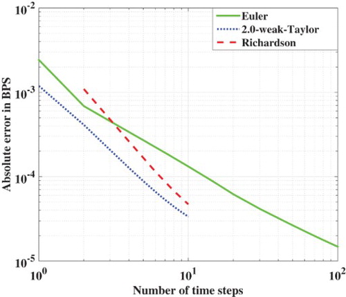
As expected, the 2.0-weak-Taylor scheme shows faster convergence than the Euler scheme, but not in terms of CPU time as we show in Table 1. This is the main disadvantage of using the 2.0-weak-Taylor scheme, and the reason why we use Richardson extrapolation on the Euler scheme which also results in a second-order method. With Richardson extrapolation, we only need two additional time steps to observe an accuracy of less than 1 BPS, compared to 2.0-weak-Taylor scheme, as is shown in Figure  1. The use of Richardson extrapolation leads to a significant reduction in CPU time.

Table 1. Number of time steps and CPU time needed to obtain an absolute error of 1 or 0.5 basis points in the Black implied volatility for the Euler (with and without Richardson extrapolation) and 2.0-weak-Taylor schemes.

	M	CPU (s)	Absolute error in BPS
Euler	28	65.41	$<1$
2.0-weak-Taylor	5	143.56	$<1$
Richardson	8	24.62	$<1$
Euler	56	134.85	$<0.5$
2.0-weak-Taylor	7	235.42	$<0.5$
Richardson	10	33.94	$<0.5$

Example 4.2.

In this example, we consider the Heston model with different values for the correlation ρ. We wish to derive the value of a European call option with initial log-asset price $x=\log \left(2\right)$, initial variance a=0.2, vol–vol $\nu =0.3$, correlations $\rho =-0.8,-0.4,0,0.4,0.8$, strike K=1.9 and time to expiration T=0.1. The reference value is obtained by using the COS method, with the ChF of the continuous process, which is given in Formula (4(4) $\begin{array}{rl}& {\phi }_{(X_{t+\mathrm{\Delta }t},A_{t+\mathrm{\Delta }t})}(u_1,u_2|X_t,A_t)\\ & =\exp \left(\mathrm{i}{u}_1{X}_t+\frac{1}{{\nu }^2}\left[\zeta \tan \left(\arctan \left[\frac{\mathrm{i}{u}_2{\nu }^2+\mathrm{i}{u}_1\rho \nu }{\zeta }\right]+\frac{\mathrm{\Delta }t}{2}\zeta \right)-\mathrm{i}{u}_1\rho \nu \right]A_t\right),\end{array}$(4) ), and with $2^{14}$ cosine coefficients. The convergence of the COS method with the Euler scheme is shown in Figure 2(a) and we observe for all values ρ first-order convergence.

Figure 2. The Heston model with different correlations: (a) the Euler–Maruyama scheme and (b) Richardson extrapolation on the Euler results.

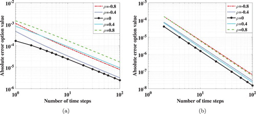
Also, we apply Richardson extrapolation on these Euler scheme results. The results are given in Figure 2(b) and we observe second-order convergence for all ρ values, confirming the accuracy of Richardson extrapolation.

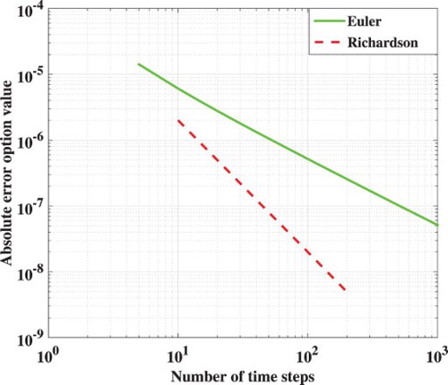
We continue by considering early-exercise dates for this problem. We take correlation $\rho =-0.2$ and we wish to derive the value of a Bermudan put option under the Heston model with strike price K=1.9 and 5 early-exercise dates: $T=0.02,0.04,0.06,0.08,0.1$. The convergence results are given in Figure 3. We observe, as expected, first-order convergence for the Euler scheme and second-order convergence with Richardson extrapolation on the Euler results. Pricing Bermudan options under the Heston model with the COS method is also considered in [14,33], and we used the method given in this last paper to obtain the reference values. The difference with our method is that we employed the ChF of the discretized process.

Figure 3. Heston Bermudan put with 5 early-exercise dates.

4.2. BSDE examples

In the first experiment, we approximate the value of a geometric basket call option and in the second example we consider a spread option. We price a European call option under the SABR model in the last experiment. All forward processes are under the $\mathbb{P}$-measure and we choose ${\theta }_1=0$ and ${\theta }_2=1$ for the Euler scheme in each example, because for these values we obtain smooth, monotonic convergence for the Euler scheme, which is a necessary condition for applying Richardson extrapolation, see also [21]. For the 2.0-weak-Taylor scheme, we take ${\theta }_1={\theta }_2=\frac{1}{2}$, because a second-order numerical integration method is required to achieve second-order convergence.

Example 4.3.

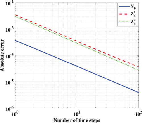
We determine the value of a geometric basket call option, where both assets follow a geometric Brownian motion (GBM): (50) $\begin{array}{r}\mathrm{d}{S}_t^1={\mu }_1{S}_t^1\mathrm{d}t+{\sigma }_1{S}_t^1\mathrm{d}{W}_t^1,S_0^1=s_1,\\ \mathrm{d}{S}_t^2={\mu }_2{S}_t^2\mathrm{d}t+\rho {\sigma }_2{S}_t^2\mathrm{d}{W}_t^1+\sqrt{1-{\rho }^2}{\sigma }_2{S}_t^2\mathrm{d}{W}_t^2,S_0^2=s_2,\end{array}$(50) and the payoff function is $g(S_T^1,S_T^2)=max(\sqrt{S_T^1}\sqrt{S_T^2}-K,0)$. For the experiment we consider the following parameter values: $\begin{array}{rl}{s}_1& =0.90,s_2=1.10,{\mu }_1=0.1,{\mu }_2=0.1,{\sigma }_1=0.2,{\sigma }_2=0.3,\rho =0.25,r=0.04,\\ K& =1,T=\mathrm{0.1.}\end{array}$

We evaluate the BSDE for pricing and hedging this basket option, such as in Formula (37(36) $\begin{array}{rl}\mathrm{d}{Y}_t& =r(Y_t-a_t^1{X}_t^1-a_t^2{X}_t^2)\mathrm{d}t+a_t^1\mathrm{d}{X}_t^1+a_t^2\mathrm{d}{X}_t^2\\ & =[r{Y}_t+({\mu }_1\left({\mathbf{\text{X}}}_t\right)-r{X}_t^1)a_t^1+({\mu }_2\left({\mathbf{\text{X}}}_t\right)-r{X}_t^2\left)a_t^2\right]\mathrm{d}t\\ & +\left[{\sigma }_1\right({\mathbf{\text{X}}}_t)a_t^1+\rho {\sigma }_2({\mathbf{\text{X}}}_t\left)a_t^2\right]\mathrm{d}{W}_t^1+\sqrt{1-{\rho }^2}{\sigma }_2\left({\mathbf{\text{X}}}_t\right)a_t^2\mathrm{d}{W}_t^2,\end{array}$(36) ), that is, (51) $\mathrm{d}{Y}_t=\left(r{Y}_t+\frac{{\mu }_1-r}{{\sigma }_1}{Z}_t^1+\frac{{\mu }_2-r}{{\sigma }_2}{Z}_t^2\right)\mathrm{d}t+(Z_t^1+\rho Z_t^2)\mathrm{d}{W}_t^1+\sqrt{1-{\rho }^2}{Z}_t^2\mathrm{d}{W}_t^2.$(51) The reference value for this option is given by the Black–Scholes price of a European call option with initial stock value $S_0=\sqrt{s_1}\sqrt{s_2}=\sqrt{0.9}\sqrt{1.1}$, constant dividend yield $q=\frac{1}{4}\left(\right({\sigma }_1{)}^2+({\sigma }_2{)}^2-2{\sigma }^2)=0.0125$, volatility $\sigma =\sqrt{\frac{1}{4}\left(\right({\sigma }_1{)}^2+({\sigma }_2{)}^2+2\rho {\sigma }_1{\sigma }_2)}=0.2$ and the same risk-free interest rate, time of maturity and strike price. This gives the reference values $Y_0=0.023982340$, $Z_0^1=0.049514739$ and $Z_0^2=0.074272109$. We observe first-order convergence of the BCOS method with the Euler scheme in Figure 4.

Figure 4. Geometric basket call option with the Euler scheme.

Example 4.4.

In this example we consider a spread option. The payoff function of such an option is given by $g(S_T^1,S_T^2)=max(S_T^1-S_T^2-K,0)$. We assume that the underlying assets both follow a constant elasticity of variance (CEV) process: (52) $\begin{array}{rl}\mathrm{d}{S}_t^1& ={\mu }_1{S}_t^1\mathrm{d}t+{\alpha }_1(S_t^1{)}^{\beta }\mathrm{d}{W}_t^1,S_0^1=s_1,\\ \mathrm{d}{S}_t^2& ={\mu }_2{S}_t^2\mathrm{d}t+\rho {\alpha }_2(S_t^2{)}^{\gamma }\mathrm{d}{W}_t^1+\sqrt{1-{\rho }^2}{\alpha }_2(S_t^2{)}^{\gamma }\mathrm{d}{W}_t^2,S_0^2=s_2,\end{array}$(52) For this example, we consider the following parameter values: $\begin{array}{rl}{s}_1& =2.1,s_2=1.9,{\mu }_1=0.1,{\mu }_2=0.1,{\alpha }_1=0.2,{\alpha }_2=0.3,\beta =0.4,\gamma =0.6,\\ \rho & =-0.2,r=0.04,K=0.2,T=\mathrm{0.1.}\end{array}$ The BSDE for pricing and hedging this spread option is given by (53) $\mathrm{d}{Y}_t=\left(r{Y}_t+\frac{{\mu }_1-r}{{\alpha }_1}(S_t^1{)}^{1-\beta }{Z}_t^1+\frac{{\mu }_2-r}{{\alpha }_2}(S_t^2{)}^{1-\gamma }{Z}_t^2\right)\mathrm{d}t+(Z_t^1+\rho Z_t^2)\mathrm{d}{W}_t^1+\sqrt{1-{\rho }^2}{Z}_t^2\mathrm{d}{W}_t^2.$(53) There is no analytic formula available for calculating the reference values. We expect to obtain similar satisfactory results for this example as for the example with GBMs in Figure 4. Therefore, we use the BCOS method with very large numbers for M and N to get the reference values $Y_0=0.0710487$, $Z_0^1=0.137419$ and $Z_0^2=-0.216524$. To double-check our results, we used Monte Carlo to obtain, respectively, the following $95\mathrm{\%}$-confidence intervals for these reference values: $[0.0698,0.0723]$, $[0.13696,0.13781]$ and $[-0.21719,-0.21573]$. The convergence of the BCOS method is shown in Figure 5, as expected we obtain first-order convergence with the Euler scheme.

Figure 5. Spread option with the Euler scheme and CEV FSDEs (52(47) $\begin{array}{rl}{Z}_m^{1,\mathrm{\Delta }}\left(\mathbf{\text{x}}\right)& =\frac{1}{\mathrm{\Delta }t{\theta }_2}{\mathbb{E}}_m\left[Y_{m+1}^{\mathrm{\Delta }}\right({\mathbf{\text{X}}}_{m+1}^{\mathrm{\Delta }}\left)\mathrm{\Delta }{W}_{m+1}^1\right]-\frac{1-{\theta }_2}{{\theta }_2}{\mathbb{E}}_m\left[Z_{m+1}^{1,\mathrm{\Delta }}\right({\mathbf{\text{X}}}_{m+1}^{\mathrm{\Delta }})+\rho Z_{m+1}^{2,\mathrm{\Delta }}({\mathbf{\text{X}}}_{m+1}^{\mathrm{\Delta }}\left)\right]\\ & +\frac{1-{\theta }_2}{{\theta }_2}{\mathbb{E}}_m\left[f\right(t_{m+1},{\mathbf{\Lambda }}_{m+1}^{\mathrm{\Delta }}\left({\mathbf{\text{X}}}_{m+1}^{\mathrm{\Delta }}\right)\left)\mathrm{\Delta }{W}_{m+1}^1\right]-\rho Z_m^{2,\mathrm{\Delta }}\left(\mathbf{\text{x}}\right),\end{array}$(47) ).

Example 4.5.

For the SABR model, we use very large numbers for M and N to get reference value $V_0$, $Z_0^1$ and $Z_0^2$, like we did in Example 4.4. In this experiment we have the following SABR FSDEs for the log-asset price $X_t^1$ and the log volatility $X_t^2$ under the $\mathbb{P}$-measure: (54) $\begin{array}{rl}\mathrm{d}{X}_t^1& =[\mu -\frac{1}{2}\exp (2X_t^2+2(\beta -1)X_t^1\left)\right]\mathrm{d}t+\exp (X_t^2+(\beta -1\left)X_t^1\right)\mathrm{d}{W}_t^1,X_0^1=x_1,\\ \mathrm{d}{X}_t^2& =-\frac{1}{2}{\nu }^2\mathrm{d}t+\rho \nu \mathrm{d}{W}_t^1+\sqrt{1-{\rho }^2}\nu \mathrm{d}{W}_t^2,X_0^2=x_2,\end{array}$(54) We make a self-financing portfolio consisting of assets $\exp \left(X_t^1\right)$, assets depending on $X_t^2$ (for example a volatility swap), and bonds and bonds.⁸ By using Formula (36(35) $\mathcal{O}\left(\right(M-1\left)N^4\right)+\mathcal{O}\left(N^2\right)+\mathcal{O}(M{N}^2\log (N\left)\right).$(35) ), we find (55) $\mathrm{d}{Y}_t=\left(r{Y}_t+\frac{\mu -r}{\exp (X_t^2+(\beta -1\left)X_t^1\right)}{Z}_t^1\right)\mathrm{d}t+(Z_t^1+\rho Z_t^2)\mathrm{d}{W}_t^1+Z_t^2\mathrm{d}{W}_t^2.$(55) For the experiment we take the following parameter values: $\begin{array}{rl}& x_1=\log \left(2\right),x_2=\log \left(0.4\right),\mu =0.2,\beta =0.8,\nu =0.4,\\ & \rho =0.25,r=0.04,K=1.9,T=\mathrm{0.1.}\end{array}$

The convergence for $Y_0$, $Z_0^1$ and $Z_0^2$ are shown in Figure 6, where we used the following reference values for the European call option: $Y_0=0.149767$, $Z_0^1=0.489597$ and $Z_0^2=0.030305$. We observe first-order convergence for the Euler scheme and second-order convergence when we use Richardson extrapolation on the Euler results. We also achieve second-order convergence with the 2.0-weak-Taylor scheme, but just as in Example 4.1, the corresponding computational costs are high. By comparing the CPU times in Tables 1 and 2, we observe that one time step with the BCOS method is around three times more expensive than one time step with the COS method. As explained in Section 3.2, these extra costs are caused by the two additional processes $Z_t^1$ and $Z_t^2$. Moreover, the 2.0-weak-Taylor scheme is also more expensive because of the use of P=10 Picard iterations per time step in the implicit Formula (46(43) $\begin{array}{rl}{Y}_m\mathrm{\Delta }{W}_{m+1}^1& =Y_{m+1}\mathrm{\Delta }{W}_{m+1}^1+{\int }_{t_m}^{t_{m+1}}f(t,{\mathbf{\Lambda }}_t)\mathrm{d}t\mathrm{\Delta }{W}_{m+1}^1-{\int }_{t_m}^{t_{m+1}}(Z_t^1+\rho Z_t^2)\mathrm{d}{W}_t^1\mathrm{\Delta }{W}_{m+1}^1\\ & -\sqrt{1-{\rho }^2}{\int }_{t_m}^{t_{m+1}}{Z}_t^2\mathrm{d}{W}_t^2\mathrm{\Delta }{W}_{m+1}^1.\end{array}$(43) ) and the additional expectations in Formulas (47(47) $\begin{array}{rl}{Z}_m^{1,\mathrm{\Delta }}\left(\mathbf{\text{x}}\right)& =\frac{1}{\mathrm{\Delta }t{\theta }_2}{\mathbb{E}}_m\left[Y_{m+1}^{\mathrm{\Delta }}\right({\mathbf{\text{X}}}_{m+1}^{\mathrm{\Delta }}\left)\mathrm{\Delta }{W}_{m+1}^1\right]-\frac{1-{\theta }_2}{{\theta }_2}{\mathbb{E}}_m\left[Z_{m+1}^{1,\mathrm{\Delta }}\right({\mathbf{\text{X}}}_{m+1}^{\mathrm{\Delta }})+\rho Z_{m+1}^{2,\mathrm{\Delta }}({\mathbf{\text{X}}}_{m+1}^{\mathrm{\Delta }}\left)\right]\\ & +\frac{1-{\theta }_2}{{\theta }_2}{\mathbb{E}}_m\left[f\right(t_{m+1},{\mathbf{\Lambda }}_{m+1}^{\mathrm{\Delta }}\left({\mathbf{\text{X}}}_{m+1}^{\mathrm{\Delta }}\right)\left)\mathrm{\Delta }{W}_{m+1}^1\right]-\rho Z_m^{2,\mathrm{\Delta }}\left(\mathbf{\text{x}}\right),\end{array}$(47) ) and (48(48) $\begin{array}{rl}{Z}_m^{2,\mathrm{\Delta }}\left(\mathbf{\text{x}}\right)& =\frac{1}{\mathrm{\Delta }t{\theta }_2\sqrt{1-{\rho }^2}}{\mathbb{E}}_m\left[Y_{m+1}^{\mathrm{\Delta }}\right({\mathbf{\text{X}}}_{m+1}^{\mathrm{\Delta }}\left)\mathrm{\Delta }{W}_{m+1}^2\right]-\frac{1-{\theta }_2}{{\theta }_2}{\mathbb{E}}_m\left[Z_{m+1}^{2,\mathrm{\Delta }}\right({\mathbf{\text{X}}}_{m+1}^{\mathrm{\Delta }}\left)\right]\\ & +\frac{1-{\theta }_2}{{\theta }_2\sqrt{1-{\rho }^2}}{\mathbb{E}}_m\left[f\right(t_{m+1},{\mathbf{\Lambda }}_{m+1}^{\mathrm{\Delta }}\left({\mathbf{\text{X}}}_{m+1}^{\mathrm{\Delta }}\right)\left)\mathrm{\Delta }{W}_{m+1}^2\right],\end{array}$(48) ) caused by ${\theta }_2=0.5$.

Figure 6. SABR example.

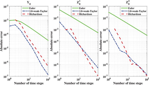
Table 2. Number of time steps and CPU time needed to obtain a certain accuracy in option price for the Euler (with and without Richardson extrapolation) and 2.0-weak-Taylor schemes.

	M	CPU (s)	Absolute error $Y_0$
Euler	12	84.95	$<3\mathrm{e}-4$
2.0-weak-Taylor	3	203.54	$<3\mathrm{e}-4$
Richardson	6	53.89	$<3\mathrm{e}-4$
Euler	36	258.43	$<1\mathrm{e}-4$
2.0-weak-Taylor	6	504.92	$<1\mathrm{e}-4$
Richardson	8	82.09	$<1\mathrm{e}-4$

5. Conclusion

In this paper, we considered the COS method for pricing European and Bermudan options and the BCOS method for solving backwards stochastic differential equations. We made use of the bivariate ChF of the discretized FSDEs in this technique, where we use the Euler-Maruyama or the 2.0-weak-Taylor scheme for the discretization. The use of these schemes in combination with the COS method results, respectively, in first-order and second-order convergence. Second-order convergence can also be observed by using Richardson extrapolation in combination with a Euler–Maruyama discretization on the forward process, which provides a significant reduction in computational costs compared to the 2.0-weak-Taylor scheme.

Disclosure statement

No potential conflict of interest was reported by the authors.

Notes

1 We omit the mean reverting term for the Heston variance.

2 From now on, we will refer to this scheme as the Euler scheme.

3 If desired, it is possible to choose $\mathrm{\Delta }t$ non-constant.

4 We left out the discount term $\exp (-r\mathrm{\Delta }t)$ for convenience.

5 For the COS method, we observe smooth, monotonic convergence for the Euler scheme, this behaviour is only observed when ${\theta }_2=1$ for the BCOS method

6 Sometimes additional assumptions are required to complete a market [8,32], such as the tradability of volatility swaps in Example 4.5.

7 In this paper, we assume a deterministic risk-free interest rate, which implies that the risk-free measure and the forward measure coincide.

8 Note that we transform $X_t^1$ and $X_t^2$, before applying the theory of Section 3.1.

Appendices

Appendix 1

In this appendix, we give the functions for Formula (6(6) $\begin{array}{rl}{X}_{m+1}^{j,\mathrm{\Delta }}& =x_j+m_j\left(\mathbf{\text{x}}\right)\mathrm{\Delta }t+s_j^1\left(\mathbf{\text{x}}\right)\mathrm{\Delta }{W}_{m+1}^1+s_j^2\left(\mathbf{\text{x}}\right)\mathrm{\Delta }{W}_{m+1}^2+{\kappa }_j^{1,2}\left(\mathbf{\text{x}}\right)\mathrm{\Delta }{W}_{m+1}^1\mathrm{\Delta }{W}_{m+1}^2\\ & +{\kappa }_j^1\left(\mathbf{\text{x}}\right)(\mathrm{\Delta }{W}_{m+1}^1{)}^2+{\kappa }_j^2(\mathbf{\text{x}}\left)\right(\mathrm{\Delta }{W}_{m+1}^2{)}^2+{\psi }_j\left(\mathbf{\text{x}}\right){\mathrm{\Psi }}_{m+1},\end{array}$(6) ) associated with the 2.0-weak-Taylor scheme. (A.1a) $\begin{array}{rl}{m}_1\left(\mathbf{\text{x}}\right)& ={\mu }_1\left(\mathbf{\text{x}}\right)-\frac{1}{2}\left({\sigma }_1\left(\mathbf{\text{x}}\right)\frac{\mathrm{\partial }{\sigma }_1\left(\mathbf{\text{x}}\right)}{\mathrm{\partial }{x}_1}+\rho {\sigma }_2\left(\mathbf{\text{x}}\right)\frac{\mathrm{\partial }{\sigma }_1\left(\mathbf{\text{x}}\right)}{\mathrm{\partial }{x}_2}\right)\\ & +\frac{1}{2}\left({\mu }_1\left(\mathbf{\text{x}}\right)\frac{\mathrm{\partial }{\mu }_1\left(\mathbf{\text{x}}\right)}{\mathrm{\partial }{x}_1}+{\mu }_2\left(\mathbf{\text{x}}\right)\frac{\mathrm{\partial }{\mu }_1\left(\mathbf{\text{x}}\right)}{\mathrm{\partial }{x}_2}+\frac{1}{2}{\sigma }_1^2\left(\mathbf{\text{x}}\right)\frac{{\mathrm{\partial }}^2{\mu }_1\left(\mathbf{\text{x}}\right)}{{\left(\mathrm{\partial }{x}_1\right)}^2}\right.\\ & +\left.\rho {\sigma }_1\left(\mathbf{\text{x}}\right){\sigma }_2\left(\mathbf{\text{x}}\right)\frac{{\mathrm{\partial }}^2{\mu }_1\left(\mathbf{\text{x}}\right)}{\mathrm{\partial }{x}_1\mathrm{\partial }{x}_2}+\frac{1}{2}{\sigma }_2^2\left(\mathbf{\text{x}}\right)\frac{{\mathrm{\partial }}^2{\mu }_1\left(\mathbf{\text{x}}\right)}{(\mathrm{\partial }{x}_2{)}^2}\right)\mathrm{\Delta }t,\end{array}$(A.1a) (A.1b) $\begin{array}{rl}{s}_1^1\left(\mathbf{\text{x}}\right)& ={\sigma }_1\left(\mathbf{\text{x}}\right)+\frac{1}{2}\left({\sigma }_1\left(\mathbf{\text{x}}\right)\frac{\mathrm{\partial }{\mu }_1\left(\mathbf{\text{x}}\right)}{\mathrm{\partial }{x}_1}+\rho {\sigma }_2\left(\mathbf{\text{x}}\right)\frac{\mathrm{\partial }{\mu }_1\left(\mathbf{\text{x}}\right)}{\mathrm{\partial }{x}_2}+{\mu }_1\left(\mathbf{\text{x}}\right)\frac{\mathrm{\partial }{\sigma }_1\left(\mathbf{\text{x}}\right)}{\mathrm{\partial }{x}_1}+{\mu }_2\left(\mathbf{\text{x}}\right)\frac{\mathrm{\partial }{\sigma }_1\left(\mathbf{\text{x}}\right)}{\mathrm{\partial }{x}_2}\right.\\ & +\left.\frac{1}{2}{\sigma }_1^2\left(\mathbf{\text{x}}\right)\frac{{\mathrm{\partial }}^2{\sigma }_1\left(\mathbf{\text{x}}\right)}{{\left(\mathrm{\partial }{x}_1\right)}^2}+\rho {\sigma }_1\left(\mathbf{\text{x}}\right){\sigma }_2\left(\mathbf{\text{x}}\right)\frac{{\mathrm{\partial }}^2{\sigma }_1\left(\mathbf{\text{x}}\right)}{\mathrm{\partial }{x}_1\mathrm{\partial }{x}_2}+\frac{1}{2}{\sigma }_2^2\left(\mathbf{\text{x}}\right)\frac{{\mathrm{\partial }}^2{\sigma }_1\left(\mathbf{\text{x}}\right)}{(\mathrm{\partial }{x}_2{)}^2}\right)\mathrm{\Delta }t,\end{array}$(A.1b) (A.1c) $s_1^2\left(\mathbf{\text{x}}\right)=\frac{\sqrt{1-{\rho }^2}}{2}{\sigma }_2\left(\mathbf{\text{x}}\right)\frac{\mathrm{\partial }{\mu }_1\left(\mathbf{\text{x}}\right)}{\mathrm{\partial }{x}_2}\mathrm{\Delta }t,{\kappa }_1^{1,2}\left(\mathbf{\text{x}}\right)=\frac{\sqrt{1-{\rho }^2}}{2}{\sigma }_2\left(\mathbf{\text{x}}\right)\frac{\mathrm{\partial }{\sigma }_1\left(\mathbf{\text{x}}\right)}{\mathrm{\partial }{x}_2},$(A.1c) (A.1d) ${\kappa }_1^1\left(\mathbf{\text{x}}\right)=\frac{1}{2}\left({\sigma }_1\left(\mathbf{\text{x}}\right)\frac{\mathrm{\partial }{\sigma }_1\left(\mathbf{\text{x}}\right)}{\mathrm{\partial }{x}_1}+\rho {\sigma }_2\left(\mathbf{\text{x}}\right)\frac{\mathrm{\partial }{\sigma }_1\left(\mathbf{\text{x}}\right)}{\mathrm{\partial }{x}_2}\right),{\kappa }_1^2\left(\mathbf{\text{x}}\right)=0,$(A.1d) (A.1e) ${\psi }_1\left(\mathbf{\text{x}}\right)=-\frac{\sqrt{1-{\rho }^2}}{2}{\sigma }_2\left(\mathbf{\text{x}}\right)\frac{\mathrm{\partial }{\sigma }_1\left(\mathbf{\text{x}}\right)}{\mathrm{\partial }{x}_2},$(A.1e) (A.1f) $\begin{array}{rl}{m}_2\left(\mathbf{\text{x}}\right)& ={\mu }_2\left(\mathbf{\text{x}}\right)-\frac{1}{2}\left(\rho {\sigma }_1\left(\mathbf{\text{x}}\right)\frac{\mathrm{\partial }{\sigma }_2\left(\mathbf{\text{x}}\right)}{\mathrm{\partial }{x}_1}+{\sigma }_2\left(\mathbf{\text{x}}\right)\frac{\mathrm{\partial }{\sigma }_2\left(\mathbf{\text{x}}\right)}{\mathrm{\partial }{x}_2}\right)\\ & +\frac{1}{2}\left({\mu }_1\left(\mathbf{\text{x}}\right)\frac{\mathrm{\partial }{\mu }_2\left(\mathbf{\text{x}}\right)}{\mathrm{\partial }{x}_1}+{\mu }_2\left(\mathbf{\text{x}}\right)\frac{\mathrm{\partial }{\mu }_2\left(\mathbf{\text{x}}\right)}{\mathrm{\partial }{x}_2}+\frac{1}{2}{\sigma }_1^2\left(\mathbf{\text{x}}\right)\frac{{\mathrm{\partial }}^2{\mu }_2\left(\mathbf{\text{x}}\right)}{{\left(\mathrm{\partial }{x}_1\right)}^2}\right.\\ & +\left.\rho {\sigma }_1\left(\mathbf{\text{x}}\right){\sigma }_2\left(\mathbf{\text{x}}\right)\frac{{\mathrm{\partial }}^2{\mu }_2\left(\mathbf{\text{x}}\right)}{\mathrm{\partial }{x}_1\mathrm{\partial }{x}_2}+\frac{1}{2}{\sigma }_2^2\left(\mathbf{\text{x}}\right)\frac{{\mathrm{\partial }}^2{\mu }_2\left(\mathbf{\text{x}}\right)}{(\mathrm{\partial }{x}_2{)}^2}\right)\mathrm{\Delta }t,\end{array}$(A.1f) (A.1g) $\begin{array}{rl}{s}_2^1\left(\mathbf{\text{x}}\right)& =\rho {\sigma }_2\left(\mathbf{\text{x}}\right)+\frac{1}{2}{\sigma }_1\left(\mathbf{\text{x}}\right)\frac{\mathrm{\partial }{\mu }_2\left(\mathbf{\text{x}}\right)}{\mathrm{\partial }{x}_1}\mathrm{\Delta }t\\ & +\frac{\rho }{2}\left({\sigma }_2\left(\mathbf{\text{x}}\right)\frac{\mathrm{\partial }{\mu }_2\left(\mathbf{\text{x}}\right)}{\mathrm{\partial }{x}_2}+{\mu }_1\left(\mathbf{\text{x}}\right)\frac{\mathrm{\partial }{\sigma }_2\left(\mathbf{\text{x}}\right)}{\mathrm{\partial }{x}_1}+{\mu }_2\left(\mathbf{\text{x}}\right)\frac{\mathrm{\partial }{\sigma }_2\left(\mathbf{\text{x}}\right)}{\mathrm{\partial }{x}_2}+\frac{1}{2}{\sigma }_1^2\left(\mathbf{\text{x}}\right)\frac{{\mathrm{\partial }}^2{\sigma }_2\left(\mathbf{\text{x}}\right)}{{\left(\mathrm{\partial }{x}_1\right)}^2}\right.\\ & +\left.\rho {\sigma }_1\left(\mathbf{\text{x}}\right){\sigma }_2\left(\mathbf{\text{x}}\right)\frac{{\mathrm{\partial }}^2{\sigma }_2\left(\mathbf{\text{x}}\right)}{\mathrm{\partial }{x}_1\mathrm{\partial }{x}_2}+\frac{1}{2}{\sigma }_2^2\left(\mathbf{\text{x}}\right)\frac{{\mathrm{\partial }}^2{\sigma }_2\left(\mathbf{\text{x}}\right)}{(\mathrm{\partial }{x}_2{)}^2}\right)\mathrm{\Delta }t,\end{array}$(A.1g) (A.1h) $\begin{array}{rl}{s}_2^2\left(\mathbf{\text{x}}\right)& =\sqrt{1-{\rho }^2}{\sigma }_2\left(\mathbf{\text{x}}\right)+\frac{\sqrt{1-{\rho }^2}}{2}\left({\sigma }_2\left(\mathbf{\text{x}}\right)\frac{\mathrm{\partial }{\mu }_2\left(\mathbf{\text{x}}\right)}{\mathrm{\partial }{x}_2}+{\mu }_1\left(\mathbf{\text{x}}\right)\frac{\mathrm{\partial }{\sigma }_2\left(\mathbf{\text{x}}\right)}{\mathrm{\partial }{x}_1}+{\mu }_2\left(\mathbf{\text{x}}\right)\frac{\mathrm{\partial }{\sigma }_2\left(\mathbf{\text{x}}\right)}{\mathrm{\partial }{x}_2}\right.\\ & +\left.\frac{1}{2}{\sigma }_1^2\left(\mathbf{\text{x}}\right)\frac{{\mathrm{\partial }}^2{\sigma }_2\left(\mathbf{\text{x}}\right)}{{\left(\mathrm{\partial }{x}_1\right)}^2}+\rho {\sigma }_1\left(\mathbf{\text{x}}\right){\sigma }_2\left(\mathbf{\text{x}}\right)\frac{{\mathrm{\partial }}^2{\sigma }_2\left(\mathbf{\text{x}}\right)}{\mathrm{\partial }{x}_1\mathrm{\partial }{x}_2}+\frac{1}{2}{\sigma }_2^2\left(\mathbf{\text{x}}\right)\frac{{\mathrm{\partial }}^2{\sigma }_2\left(\mathbf{\text{x}}\right)}{(\mathrm{\partial }{x}_2{)}^2}\right)\mathrm{\Delta }t,\end{array}$(A.1h) (A.1i) ${\kappa }_2^{1,2}\left(\mathbf{\text{x}}\right)=\frac{\sqrt{1-{\rho }^2}}{2}\left({\sigma }_1\left(\mathbf{\text{x}}\right)\frac{\mathrm{\partial }{\sigma }_2\left(\mathbf{\text{x}}\right)}{\mathrm{\partial }{x}_1}+2\rho {\sigma }_2\left(\mathbf{\text{x}}\right)\frac{\mathrm{\partial }{\sigma }_2\left(\mathbf{\text{x}}\right)}{\mathrm{\partial }{x}_2}\right),$(A.1i) (A.1j) ${\kappa }_2^1\left(\mathbf{\text{x}}\right)=\frac{\rho }{2}\left({\sigma }_1\left(\mathbf{\text{x}}\right)\frac{\mathrm{\partial }{\sigma }_2\left(\mathbf{\text{x}}\right)}{\mathrm{\partial }{x}_1}+\rho {\sigma }_2\left(\mathbf{\text{x}}\right)\frac{\mathrm{\partial }{\sigma }_2\left(\mathbf{\text{x}}\right)}{\mathrm{\partial }{x}_2}\right),$(A.1j) (A.1k) ${\kappa }_2^2\left(\mathbf{\text{x}}\right)=\frac{1-{\rho }^2}{2}{\sigma }_2\left(\mathbf{\text{x}}\right)\frac{\mathrm{\partial }{\sigma }_2\left(\mathbf{\text{x}}\right)}{\mathrm{\partial }{x}_2},{\psi }_2\left(\mathbf{\text{x}}\right)=\frac{\sqrt{1-{\rho }^2}}{2}{\sigma }_1\left(\mathbf{\text{x}}\right)\frac{\mathrm{\partial }{\sigma }_2\left(\mathbf{\text{x}}\right)}{\mathrm{\partial }{x}_1}.$(A.1k)

Appendix 2

In this appendix, we provide some information on how to choose the computational domain $[a_1,b_1]\times [a_2,b_2]$. The FSDEs are given by Formula (1(1) $\begin{array}{rl}\mathrm{d}{X}_t^1& ={\mu }_1(X_t^1,X_t^2)\mathrm{d}t+{\sigma }_1(X_t^1,X_t^2)\mathrm{d}{W}_t^1,\\ \mathrm{d}{X}_t^2& ={\mu }_2(X_t^1,X_t^2)\mathrm{d}t+\rho {\sigma }_2(X_t^1,X_t^2)\mathrm{d}{W}_t^1+\sqrt{1-{\rho }^2}{\sigma }_2(X_t^1,X_t^2)\mathrm{d}{W}_t^2,\end{array}$(1) ), that is, (A.2) $\begin{array}{rl}\mathrm{d}{X}_t^1& ={\mu }_1\left({\mathbf{\text{X}}}_t\right)\mathrm{d}t+{\sigma }_1\left({\mathbf{\text{X}}}_t\right)\mathrm{d}{W}_t^1,\\ \mathrm{d}{X}_t^2& ={\mu }_2\left({\mathbf{\text{X}}}_t\right)\mathrm{d}t+\rho {\sigma }_2\left({\mathbf{\text{X}}}_t\right)\mathrm{d}{W}_t^1+\sqrt{1-{\rho }^2}{\sigma }_2\left({\mathbf{\text{X}}}_t\right)\mathrm{d}{W}_t^2,\end{array}$(A.2) where $X_0^1=x_1$ and $X_0^2=x_2$.

When the first, second and fourth cumulants of $X_T^1$ and $X_T^2$ given $(x_1,x_2)$ are known we advise to choose the domain $[a_1,b_1]\times [a_2,b_2]$ as presented in [33], so for i=1,2: (A.3) $[a_i,b_i]=[x_i+c_{i,1}-L\sqrt{c_{i,2}+\sqrt{c_{i,4}}},x_i+c_{i,1}+L\sqrt{c_{i,2}+\sqrt{c_{i,4}}}],$(A.3) where L=10 and $c_{i,j}$ denotes the j-th cumulant of $X_T^i$ given $(x_1,x_2)$. When the first cumulant is relatively large, we suggest to use a time-dependent domain, that is, (A.4) $\left[a_i\right(t),b_i(t\left)\right]=[x_i+c_{i,1}(t)-L\sqrt{c_{i,2}\left(t\right)+\sqrt{c_{i,4}\left(t\right)}},x_i+c_{i,1}(t)+L\sqrt{c_{i,2}\left(t\right)+\sqrt{c_{i,4}\left(t\right)}}],$(A.4) where $c_{i,j}\left(t\right)$ denotes the j-th cumulant of $X_t^i$ given $(x_1,x_2)$. This time dependency is important, because otherwise, for example $x_i$ may be outside the interval $[a_i,b_i]$. The (B)COS method only needs a minor adaptation regarding the time-dependent domain: $a_i$ and $b_i$ have to be replaced by $a_i\left(t_m\right)$ and $b_i\left(t_m\right)$, respectively, in Formulas (25(25) $\begin{array}{rl}{V}_m^{\mathrm{\Delta }}\left(\mathbf{\text{x}}\right)& \approx \underset{k_1=0}{\overset{N-1}{{\sum }^{\prime }}}\underset{k_2=0}{\overset{N-1}{{\sum }^{\prime }}}\frac{1}{2}\mathrm{\Re }\left\{{\phi }_{{\mathbf{\text{X}}}_{m+1}^{\mathrm{\Delta }}}\left(\left.\frac{k_1\pi }{b_1-a_1},\frac{k_2\pi }{b_2-a_2}\right|\mathbf{\text{x}}\right)\exp \left(-\mathrm{i}{k}_1\pi \frac{a_1}{b_1-a_1}-\mathrm{i}{k}_2\pi \frac{a_2}{b_2-a_2}\right)\right.\\ & +\left.{\phi }_{{\mathbf{\text{X}}}_{m+1}^{\mathrm{\Delta }}}\left(\left.\frac{k_1\pi }{b_1-a_1},-\frac{k_2\pi }{b_2-a_2}\right|\mathbf{\text{x}}\right)\exp \left(-\mathrm{i}{k}_1\pi \frac{a_1}{b_1-a_1}+i{k}_2\pi \frac{a_2}{b_2-a_2}\right)\right\}{\mathcal{V}}_{k_1,k_2},\end{array}$(25) ), (26(26) ${\mathcal{V}}_{k_1,k_2}=\frac{2}{b_1-a_1}\frac{2}{b_2-a_2}{\int }_{a_2}^{b_2}{\int }_{a_1}^{b_1}{V}_{m+1}^{\mathrm{\Delta }}\left(\mathbf{\text{X}}\right)\cos \left(k_1\pi \frac{X_1-a_1}{b_1-a_1}\right)\cos \left(k_2\pi \frac{X_2-a_2}{b_2-a_2}\right)\mathrm{d}{X}_1\mathrm{d}{X}_2.$(26) ) and in each formula in Appendix 3.

When the cumulants of $X_T^1$ and/or $X_T^2$ given $(x_1,x_2)$ are unknown, we choose the domain as in [36]: (A.5) $[a_i,b_i]=[c_{i,1}-L\sqrt{c_{i,2}},c_{i,1}+L\sqrt{c_{i,2}}],$(A.5) where L=10, $c_{i,1}=x_i+{\mu }_i(x_1,x_2)T$ and $c_{i,2}={\sigma }_i(x_1,x_2)T$. When desired, this domain can also be time dependent. The interval $[a_i,b_i]$ can be adjusted such that it satisfies specific constraints of $X_t^i$, for example, non-negativity.

We used Equation (A.5) for all experiments for the SABR model, but not for problems in which a drift function is large compared to the associated volatility, for example, (A.6) $\begin{array}{rl}\mathrm{d}{X}_t& ={\alpha }_t\mathrm{d}t,X_0=x,\\ \mathrm{d}{\alpha }_0& =\gamma {\alpha }_t\mathrm{d}{W}_t,{\sigma }_0=\alpha ,\end{array}$(A.6) where W is a standard Brownian motion and the vol–vol parameter $\gamma \ge 0$.

If we follow Equation (A.5), we would obtain (A.7) $\left[a_1\right(t),b_1(t\left)\right]=x+\alpha t.$(A.7) This is incorrect, because $X_t$ is not deterministic.

A better domain $\left[a_1\right(t),b_1(t\left)\right]\times \left[a_2\right(t),b_2(t\left)\right]$ in this case would be based on Formula (A.5), as follows: (A.8) $\left[a_2\right(t),b_2(t\left)\right]=[max\{0,\alpha -L\gamma \alpha \sqrt{t}\},\alpha +L\gamma \alpha \sqrt{t}],$(A.8) so that we find (A.9) $X_t\ge x+{\int }_0^t{a}_2\left(t\right)\mathrm{d}t=a_1\left(t\right),$(A.9) and (A.10) $X_t\le x+{\int }_0^t{b}_2\left(t\right)\mathrm{d}t=x+\alpha t+\frac{2}{3}L\gamma \alpha t^{3/2}=b_1\left(t\right).$(A.10)

Appendix 3

In this appendix, we give approximations of ${\mathbb{E}}_m\left[h\right(t_{m+1},{\mathbf{\text{X}}}_{m+1}^{\mathrm{\Delta }}\left)\right]$, ${\mathbb{E}}_m\left[h\right(t_{m+1},{\mathbf{\text{X}}}_{m+1}^{\mathrm{\Delta }}\left)\mathrm{\Delta }{W}_{m+1}^1\right]$ and ${\mathbb{E}}_m\left[h\right(t_{m+1},{\mathbf{\text{X}}}_{m+1}^{\mathrm{\Delta }}\left)\mathrm{\Delta }{W}_{m+1}^2\right]$ with the COS method for a general sufficiently smooth function $h(t,\mathbf{\text{x}})$. We denote (A.11) ${\mathcal{H}}_{k_1,k_2}\left(t_{m+1}\right)=\frac{2}{b_1-a_1}\frac{2}{b_2-a_2}{\int }_{a_2}^{b_2}{\int }_{a_1}^{b_1}h(t_{m+1},\mathbf{\text{x}})\cos \left(k_1\pi \frac{x_1-a_1}{b_1-a_1}\right)\cos \left(k_2\pi \frac{x_2-a_2}{b_2-a_2}\right)\mathrm{d}{x}_1\mathrm{d}{x}_2.$(A.11) Using the two-dimensional COS method, we find (A.12) $\begin{array}{rl}& {\mathbb{E}}_m\left[h\right(t_{m+1},{\mathbf{\text{X}}}_{m+1}^{\mathrm{\Delta }}\left)\right]\\ & \approx \underset{k_1=0}{\overset{N_1-1}{{\sum }^{\prime }}}\underset{k_2=0}{\overset{N_2-1}{{\sum }^{\prime }}}\frac{1}{2}\mathrm{\Re }\left\{{\phi }_{{\mathbf{\text{X}}}_{m+1}^{\mathrm{\Delta }}}\left(\left.\frac{k_1\pi }{b_1-a_1},\frac{k_2\pi }{b_2-a_2}\right|{\mathbf{\text{X}}}_m^{\mathrm{\Delta }}=\mathbf{\text{x}}\right)\exp \left(-\mathrm{i}{k}_1\pi \frac{a_1}{b_1-a_1}-\mathrm{i}{k}_2\pi \frac{a_2}{b_2-a_2}\right)\right.\\ & +\left.{\phi }_{{\mathbf{\text{X}}}_{m+1}^{\mathrm{\Delta }}}\left(\left.\frac{k_1\pi }{b_1-a_1},-\frac{k_2\pi }{b_2-a_2}\right|{\mathbf{\text{X}}}_m^{\mathrm{\Delta }}=\mathbf{\text{x}}\right)\exp \left(-\mathrm{i}{k}_1\pi \frac{a_1}{b_1-a_1}+\mathrm{i}{k}_2\pi \frac{a_2}{b_2-a_2}\right)\right\}{\mathcal{H}}_{k_1,k_2}\left(t_{m+1}\right).\end{array}$(A.12) Also, we have (A.13) $\begin{array}{rl}& {\mathbb{E}}_m\left[h\right(t_{m+1},{\mathbf{\text{X}}}_{m+1}^{\mathrm{\Delta }}\left)\mathrm{\Delta }{W}_{m+1}^1\right]\\ & \approx \underset{k_1=0}{\overset{N_1-1}{{\sum }^{\prime }}}\underset{k_2=0}{\overset{N_2-1}{{\sum }^{\prime }}}\frac{1}{2}\mathrm{\Re }\left\{(i{d}_1^{+}\mathrm{\Delta }t-d_2^{+}{d}_3^{+}(\mathrm{\Delta }t{)}^2-2d_1^{+}{d}_4^{+}\left(\mathrm{\Delta }t{)}^2\right){\phi }_{{\mathbf{\text{X}}}_{m+1}^{\mathrm{\Delta }}}\left(\left.\frac{k_1\pi }{b_1-a_1},\frac{k_2\pi }{b_2-a_2}\right|{\mathbf{\text{X}}}_m^{\mathrm{\Delta }}=\mathbf{\text{x}}\right)\right.\\ & \cdot \exp \left(-i{k}_1\pi \frac{a_1}{b_1-a_1}-\mathrm{i}{k}_2\pi \frac{a_2}{b_2-a_2}\right)+(i{d}_1^{-}\mathrm{\Delta }t-d_2^{-}{d}_3^{-}(\mathrm{\Delta }t{)}^2-2d_1^{-}{d}_4^{-}\left(\mathrm{\Delta }t{)}^2\right)\\ & \cdot \left.{\phi }_{{\mathbf{\text{X}}}_{m+1}^{\mathrm{\Delta }}}\left(\left.\frac{k_1\pi }{b_1-a_1},-\frac{k_2\pi }{b_2-a_2}\right|{\mathbf{\text{X}}}_m^{\mathrm{\Delta }}=\mathbf{\text{x}}\right)\exp \left(-\mathrm{i}{k}_1\pi \frac{a_1}{b_1-a_1}+\mathrm{i}{k}_2\pi \frac{a_2}{b_2-d_2}\right)\right\}{\mathcal{H}}_{k_1,k_2}\left(t_{m+1}\right),\end{array}$(A.13) and (A.14) $\begin{array}{rl}& {\mathbb{E}}_m\left[h\right(t_{m+1},{\mathbf{\text{X}}}_{m+1}^{\mathrm{\Delta }}\left)\mathrm{\Delta }{W}_{m+1}^2\right]\\ & \approx \underset{k_1=0}{\overset{N_1-1}{{\sum }^{\prime }}}\underset{k_2=0}{\overset{N_2-1}{{\sum }^{\prime }}}\frac{1}{2}\mathrm{\Re }\left\{(i{d}_2^{+}\mathrm{\Delta }t-d_1^{+}{d}_3^{+}(\mathrm{\Delta }t{)}^2-2d_2^{+}{d}_5^{+}\left(\mathrm{\Delta }t{)}^2\right){\phi }_{{\mathbf{\text{X}}}_{m+1}^{\mathrm{\Delta }}}\left(\left.\frac{k_1\pi }{b_1-a_1},\frac{k_2\pi }{b_2-a_2}\right|{\mathbf{\text{X}}}_m^{\mathrm{\Delta }}=\mathbf{\text{x}}\right)\right.\\ & \cdot \exp \left(-\mathrm{i}{k}_1\pi \frac{a_1}{b_1-a_1}-\mathrm{i}{k}_2\pi \frac{a_2}{b_2-a_2}\right)+(i{d}_2^{-}\mathrm{\Delta }t-d_1^{-}{d}_3^{-}(\mathrm{\Delta }t{)}^2-2d_2^{-}{d}_5^{-}\left(\mathrm{\Delta }t{)}^2\right)\\ & \cdot \left.{\phi }_{{\mathbf{\text{X}}}_{m+1}^{\mathrm{\Delta }}}\left(\left.\frac{k_1\pi }{b_1-a_1},-\frac{k_2\pi }{b_2-a_2}\right|{\mathbf{\text{X}}}_m^{\mathrm{\Delta }}=\mathbf{\text{x}}\right)\exp \left(-i{k}_1\pi \frac{a_1}{b_1-a_1}+i{k}_2\pi \frac{a_2}{b_2-a_2}\right)\right\}{\mathcal{H}}_{k_1,k_2}\left(t_{m+1}\right),\end{array}$(A.14) where we abbreviated: (A.15) $\begin{array}{rl}{d}_1^{\pm }& =\frac{k_1\pi }{b_1-a_1}{s}_1^1\left(\mathbf{\text{x}}\right)\pm \frac{k_2\pi }{b_2-a_2}{s}_2^1\left(\mathbf{\text{x}}\right),d_4^{\pm }=\frac{k_1\pi }{b_1-a_1}{\kappa }_1^1\left(\mathbf{\text{x}}\right)\pm \frac{k_2\pi }{b_2-a_2}{\kappa }_2^1\left(\mathbf{\text{x}}\right),\\ d_2^{\pm }& =\frac{k_1\pi }{b_1-a_1}{s}_1^2\left(\mathbf{\text{x}}\right)\pm \frac{k_2\pi }{b_2-a_2}{s}_2^2\left(\mathbf{\text{x}}\right),d_5^{\pm }=\pm \frac{k_2\pi }{b_2-a_2}{\kappa }_2^2\left(\mathbf{\text{x}}\right),\\ d_3^{\pm }& =\frac{k_1\pi }{b_1-a_1}{\kappa }_1^{1,2}\left(\mathbf{\text{x}}\right)\pm \frac{k_2\pi }{b_2-a_2}{\kappa }_2^{1,2}\left(\mathbf{\text{x}}\right).\end{array}$(A.15) The approximations (A.13) and (A.14) have, besides the error introduced by the COS method, an error of order $\mathcal{O}\left(\right(\mathrm{\Delta }t{)}^3)$ [36].

References

- A. Antonov, M. Konikov, and M. Spector, SABR spreads its wings, Risk (2013), pp. 58–63.
- P. Balland and Q. Tran, SABR goes normal, Risk (2013), pp. 76–81.
- F. Black and M. Scholes, The pricing of options and corporate liabilities, J. Polit. Econ. 81(3) (1973), pp. 637–654.
- B. Bouchard and N. Touzi, Discrete-time approximation and Monte-Carlo simulation of backward stochastic differential equations, Stochastic Processes Appl. 11(2) (2004), pp. 175–206.
- P.P. Boyle, Options: A Monte Carlo approach, J. Financ. Econ. 4 (1977), pp. 323–338.
- P. Carr and D.B. Madan, Option valuation using the fast Fourier transform, J. Comput. Finance 2 (1999), pp. 61–73.
- D. Chen, H.J. Harkonen, and D.P. Newton, Advancing the universality of quadrature methods to any underlying process for option pricing, J. Finan. Econ. 114(3) (2014), pp. 600–612.
- M.H.A. Davis, Complete-market models of stochastic volatility, Proc. Roy. Soc. A 460(2041) (2004), pp. 11–26.
- P. Doust, No-arbitrage SABR, J. Comput. Finance 15(3) (2012), pp. 3–31.
- D.J. Duffy, Finite Difference Methods in Financial Engineering: A Partial Differential Equation Approach, Wiley, Chichester, 2006.
- N. El Karoui, S. Peng, and M.C. Quenez, Backward stochastic differential equations in finance, Math. Finance 7(1) (1997), pp. 1–71.
- F. Fang and C.W. Oosterlee, A novel pricing method for European option based on Fourier-cosine series expansions, SIAM J. Sci. Comput. 31(2) (2008), pp. 826–848.
- F. Fang and C.W. Oosterlee, Pricing early-exercise and discrete barrier options by Fourier-cosine series expansions, Numer. Math. 114(1) (2009), pp. 27–62.
- F. Fang and C.W. Oosterlee, A Fourier-based valuation method for Bermudan and barrier options under Heston's model, SIAM J. Finan. Math. 2 (2011), pp. 439–463.
- P. Glasserman, Monte Carlo Methods in Financial Engineering, Springer-Verlag, New York, 2003.
- L.A. Grzelak and C.W. Oosterlee, From arbitrage to arbitrage-free implied volatilities, J. Comput. Finance 20 (2016), pp. 1–19.
- P.S. Hagan, D. Kumar, A.S. Lesniewski, and D.E. Woodward, Managing smile risk, Wilmott Mag. (2002), pp. 84–108.
- P.S. Hagan, D. Kumar, A.S. Lesniewski, and D.E. Woodward, Arbitrage-free SABR, Wilmott Mag. (2014), pp. 60–75.
- S.L. Heston, A closed-form solution for options with stochastic volatility with applications to bond and currency options, Rev. Finan. Stud. 6(2) (1993), pp. 327–343.
- D.J. Higham, An introduction to multilevel Monte Carlo for option valuation, Int. J. Comput. Math. 92(12) (2015), pp. 2347–2360.
- T.P. Huijskens, M.J. Ruijter, and C.W. Oosterlee, Efficient numerical Fourier methods for coupled forward–backward SDEs, J. Comput. Appl. Math. 296 (2016), pp. 593–612.
- K.J. in 't Hout and S. Foulon, ADI finite difference schemes for option pricing in the Heston model with correlation, Int. J. Numer. Anal. Modeling 7(2) (2010), pp. 303–320.
- A. Khedher and M. Vanmaele, Discretisation of FBSDEs driven by cádlág martingales, J. Math. Anal. Appl. 435(1) (2016), pp. 508–531.
- P.E. Kloeden and E. Platen, Numerical Solution of Stochastic Differential Equations, Springer-Verlag, Berlin, 1992.
- A.L. Lewis, A simple option formula for general jump-diffusion and other exponential Lévy processes, SSRN Paper, 2001.
- A. Lipton, Mathematical Methods for Foreign Exchange: A Financial Engineer's Approach, World Scientific, Singapore, 2001.
- J. Obłój, Fine-Tune Your Smile: Correction to Hagan et al, Wilmott Mag. (2008), pp. 102–104.
- L. Ortiz-Gracia and C.W. Oosterlee, Robust pricing of European options with wavelets and the characteristic function, SIAM J. Sci. Comput. 35(5) (2013), pp. B1055–B1084.
- E. Pardoux and S.G. Peng, Adapted solution of a backward stochastic differential equation, Syst. Control Lett. 14(1) (1990), pp. 55–61.
- E. Pardoux and S.G. Peng, Backward stochastic differential equations and quasilinear parabolic partial differential equations, in Stochastic Partial Differential Equations and Their Applications, B.L. Rozovskii and R.B. Sowers, eds., Lecture Notes in Control and Information Sciences, Vol. 176, Springer, Berlin, 1992, pp. 200–217.
- H. Park, Efficient valuation method for the SABR model, SSRN Paper, 2013.
- C.W. Potter, Complete stochastic volatility models with variance swaps, Tech. Rep., 2004.
- M.J. Ruijter and C.W. Oosterlee, Two-dimensional Fourier cosine series expansion method for pricing financial options, SIAM J. Sci. Comput. 34(5) (2012), pp. B642–B671.
- M.J. Ruijter and C.W. Oosterlee, A Fourier-cosine method for an efficient computation of solutions to BSDEs, SIAM J. Sci. Comput. 37(2) (2015), pp. A859–A889.
- M.J. Ruijter and C.W. Oosterlee, Numerical Fourier method and second-order Taylor scheme for backward SDEs in finance, Appl. Numer. Math. 103 (2016), pp. 1–26.
- Z. van der Have, Arbitrage-free methods to price European options under the SABR model, Master's thesis, TU Delft, 2015.
- L. von Sydow, L.J. Höök, E. Larsson, E. Lindström, S. Milovanović, J. Persson, V. Shcherbakov, Y. Shpolyanskiy, S. Sirén, J. Toivanen, J. Waldén, M. Wiktorsson, M.B. Giles, J. Levesley, J. Li, C.W. Oosterlee, M.J. Ruijter, A. Toropov, and Y. Zhao, BENCHOP: The BENCHmarking project in Option Pricing, Int. J. Comput. Math. 92(12) (2015), pp. 2361–2379.
- W. Zhao, L. Chen, and S. Peng, A new kind of accurate numerical method for backward stochastic differential equations, SIAM J. Sci. Comput. 28(4) (2006), pp. 1563–1581.