A new two-sided projection technique for model reduction of quadratic-bilinear descriptor systems

ABSTRACT

We investigate the problem of projection-based interpolation for model reduction of quadratic-bilinear descriptor systems. Existing two-sided projection techniques are analysed and a modified sequence of projection matrices is proposed. It is observed that the proposed technique generates better reduced order systems. Numerical results for some benchmark examples are presented in support of our observation.

Keywords:

• Model order reduction
• quadratic-bilinear systems
• two-sided projection
• descriptor systems
• multivariable transfer function

2010 Mathematics Subject Classifications:

• 65F99
• 65L80

1. Introduction

The problem of model reduction is to compute a reduced system for a given system such that the responses to all feasible excitations of the two systems are comparable and the size of the reduced system allows the use of simulation, control and optimization in a computationally efficient way. We consider model reduction techniques for a single-input single-output quadratic-bilinear descriptor system of the form: (1) $\begin{array}{rl}E\dot{x}\left(t\right)& =Ax\left(t\right)+Nx\left(t\right)u\left(t\right)+Qx\left(t\right)\otimes x\left(t\right)+Bu\left(t\right),\\ y\left(t\right)& =Cx\left(t\right),\end{array}$(1) where $E,A,N\in {\mathbb{R}}^{n\times n}$, $Q\in {\mathbb{R}}^{n\times n^2}$, $B,C^{\mathrm{T}}\in {\mathbb{R}}^n$ are the system matrices. $x\left(t\right)\in {\mathbb{R}}^n$ is the state vector and $u\left(t\right),y\left(t\right)\in \mathbb{R}$ are the input and output of the system, respectively. In addition to systems that naturally appear in the quadratic-bilinear form such as certain discretized Burgers and Navier–Stokes equations, a large class of nonlinear systems can be written in to quadratic-bilinear form by using exact transformations [14]. Model order reduction (MOR) of such nonlinear systems constructs a reduced system of dimension $r\ll n$ with structure similar to that in (1(1) $\begin{array}{rl}E\dot{x}\left(t\right)& =Ax\left(t\right)+Nx\left(t\right)u\left(t\right)+Qx\left(t\right)\otimes x\left(t\right)+Bu\left(t\right),\\ y\left(t\right)& =Cx\left(t\right),\end{array}$(1) ). That is (2) $\begin{array}{rl}{E}_r{\dot{x}}_r\left(t\right)& =A_r{x}_r\left(t\right)+N_r{x}_r\left(t\right)u\left(t\right)+Q_r{x}_r\left(t\right)\otimes x_r\left(t\right)+B_{r}u\left(t\right),\\ y_r\left(t\right)& =C_r{x}_r\left(t\right).\end{array}$(2) The reduction approach should ensure that the output response $y_r\left(t\right)$ approximates $y\left(t\right)$ to a certain accuracy. Various techniques have been proposed in the literature to compute such reduced order models, cf., [2, 7]. Here, we discuss projection-based interpolatory techniques [3, 13] that are widely used in the linear case and are recently extended to quadratic-bilinear systems [1, 6, 14].

Projection involves the following steps:

1. Approximate the state vector: $x\left(t\right)\approx V{x}_r\left(t\right)$, where $V\in {\mathbb{R}}^{n\times r}$.

2. Ensure Petrov–Galerkin orthogonality condition on the residual:

3. $W^{\mathrm{T}}r\left(t\right)=0$, where $W\in {\mathbb{R}}^{n\times r}$ and $r\left(t\right)=EV{\dot{x}}_r\left(t\right)-\left(AV{x}_r\left(t\right)+NV{x}_r\left(t\right)u\left(t\right)+QV{x}_r\left(t\right)\otimes V{x}_r\left(t\right)+Bu\left(t\right)\right)$ is the residual.

The projection is orthogonal if W=V and is often called one-sided projection, otherwise it is oblique and called two-sided projection. The oblique projection framework leads to a set of reduced system matrices of the form: (3) $\begin{array}{rl}{E}_r=W^{\mathrm{T}}EV,A_r& =W^{\mathrm{T}}AV,Q_r=W^{\mathrm{T}}Q(V\otimes V),N_r=W^{\mathrm{T}}NV,\\ B_r& =W^{\mathrm{T}}B,C_r=CV.\end{array}$(3) The important question is how to compute the basis matrices V and W. Analogous to the linear case, the choice of the basis matrices V and W can be linked to the input–output representation of the system. However, quadratic-bilinear systems involve a series of multivariate transfer functions, each representing a subsystem of the original system. Thus the problem is how to construct V and W such that the first K multivariate transfer functions associated with the reduced system are interpolating the corresponding original multivariate transfer functions, at multiple frequency shifts. To achieve this, orthogonal projections [14] as well as oblique projections [1, 6] have been used in the literature with some simplifications. For example, the approach in [6] constructs V and W such that the reduced system ensures interpolation of the first two subsystems only. Also the choice of interpolation points for each frequency variable is assumed to be the same. The method in [1] identified a simplified structure of the generalized transfer functions, which allowed us to avoid the above simplifications. However, it can be observed that for systems with dominant quadratic part, the symmetric structure of the generalized transfer functions used in [6] is more stable. Therefore, our focus in this paper is on the moment matching of symmetric generalized transfer functions. We discuss these results further in Section 2.

Recently a new framework [9] for quadratic-bilinear systems has been proposed that is based on generalized Sylvester-type matrix equations. The approach involves truncated solution of two complex matrix equations to identify a good choice for the basis matrices V and W. The idea in [9] is motivated from the bilinear reduction techniques [4, 11] and the weighted sum of the generalized transfer functions for quadratic-bilinear systems is regarded. It is not clear how the quasi-optimal shift frequencies are interpolating the individual generalized transfer functions [6, 14]. Moreover, the construction of the ${\mathcal{H}}_2$-quasi-optimal truncation matrices is quite time-consuming, leading to large offline times for constructing the reduced order model. Our target in this paper is to interpolate, separately, the first two or three generalized transfer functions, so that multiple moment matching techniques can also be utilized for model order reduction of quadratic-bilinear systems. The involved computations will in general require much less computational resources than the technique from [9]. Therefore in what follows we will mainly focus on the two-sided moment matching technique of Benner and Breiten [6].

In this paper, we use a modified sequence of column spaces in the basis matrices V and W and prove the multi-moment matching properties of the resulting reduced order system. Besides the multi-moment matching achieved in [6], the modified sequences ensure that the derivative of the first subsystem is also matched by the reduced system. The choice of the interpolation points or shift frequencies is random or linked to the linear part of the system (using IRKA [15] on $(E,A,B,C)$).

The remaining part of the paper is organized as follows. Section 2 shows the transfer function representation for quadratic-bilinear systems and the existing multi-moment matching framework. Section 3 introduces the modified form of the multi-moment matching approach. Section 4 shows numerical results for some benchmark examples. Finally we present the conclusions and future work.

2. Background

In this section, we briefly review the concept of moment matching discussed in [1, 6] for quadratic-bilinear systems. Before going into the details of nonlinear moment matching, we begin with the structure of high-order transfer functions.

2.1. Multivariate transfer functions

The input–output representation for the system in (1(1) $\begin{array}{rl}E\dot{x}\left(t\right)& =Ax\left(t\right)+Nx\left(t\right)u\left(t\right)+Qx\left(t\right)\otimes x\left(t\right)+Bu\left(t\right),\\ y\left(t\right)& =Cx\left(t\right),\end{array}$(1) ) can be expressed by the Volterra series expansion of the output $y\left(t\right)$ with quantities analogous to the standard convolution operator. That is, (4) $y\left(t\right)=c\sum _{k=1}^{\mathrm{\infty }}{\int }_0^t{\int }_0^{t_1}\cdots {\int }_0^{t_{k-1}}{h}_k(t_1,\dots ,t_k)u(t-t_1)\cdots u(t-t_k)\mathrm{d}{t}_k\cdots \mathrm{d}{t}_1,$(4) where it is assumed that the input signal is one-sided, $u\left(t\right)=0$ for t<0. In addition, each of the generalized impulse responses, $h_k(t_1,\dots ,t_k)$, also called the k-dimensional kernel of the subsystem, is assumed to be one-sided. In terms of the multivariable Laplace transform, the k-dimensional subsystem can be represented as (5) $Y_k(s_1,\dots ,s_k)=H_k(s_1,\dots ,s_k)U\left(s_1\right)\cdots U\left(s_k\right),$(5) where $H_k(s_1,\dots ,s_k)$ is the multivariable transfer function of the k-dimensional subsystem and $s_i\in \mathbb{C}$ for $i=1,\dots ,k$. The structure of the generalized transfer functions can be identified by the growing exponential approach [19]. To this end, we assume that the matrix pencil sE−A is regular, i.e. sE−A is singular only for finitely many values of $s\in \mathbb{C}$ [12]. The first three transfer functions of the quadratic-bilinear system (1(1) $\begin{array}{rl}E\dot{x}\left(t\right)& =Ax\left(t\right)+Nx\left(t\right)u\left(t\right)+Qx\left(t\right)\otimes x\left(t\right)+Bu\left(t\right),\\ y\left(t\right)& =Cx\left(t\right),\end{array}$(1) ) can be written as (6) $\begin{array}{rl}{H}_1\left(s_1\right)& =C(s_{1}E-A{)}^{-1}B,\\ H_2(s_1,s_2)& =C\left(\right(s_1+s_2)E-A{)}^{-1}X(s_1,s_2),\\ H_3(s_1,s_2,s_3)& =C\left(\right(s_1+s_2+s_3)I-A{)}^{-1}X(s_1,s_2,s_3),\end{array}$(6) where (7) $\begin{array}{rl}X(s_1,s_2)& :=Q\left(X_1\right(s_1)\otimes X_1(s_2\left)\right)+\frac{1}{2!}N\left(X_1\right(s_1)+X_1(s_2\left)\right),\\ X(s_1,s_2,s_3)& :=\frac{1}{3!}N\left[X_2(s_1,s_2)+X_2(s_2,s_3)+X_2(s_1,s_3)\right]\\ & +\frac{1}{3}Q\left[X_1\left(s_1\right)\otimes X_2(s_2,s_3)+X_1\left(s_2\right)\otimes X_2(s_1,s_3)\right.\\ & \left.+X_1\left(s_3\right)\otimes X_2(s_1,s_2)\right],\end{array}$(7) in which $X_1\left(s\right):=(sE-A{)}^{-1}B$, $X_2(s_1,s_2):=\left(\right(s_1+s_2)E-A{)}^{-1}X(s_1,s_2)$ and Q satisfies $Q(u\otimes v)=Q(v\otimes u)$ for all $u,v\in {\mathbb{R}}^n$. Similarly, if we define $X_3(s_1,s_2,s_3):=\left(\right(s_1+s_2+s_3)E-A{)}^{-1}X(s_1,s_2,s_3)$, the first three symmetric transfer functions can be written as $\begin{array}{r}\begin{array}{rl}{H}_1\left(s_1\right)& =C{X}_1\left(s_1\right),H_2(s_1,s_2)=C{X}_2(s_1,s_2),\\ H_3(s_1,s_2,s_3)& =C{X}_3(s_1,s_2,s_3).\end{array}\end{array}$ Before going into the partial differentiation of the multivariate transfer functions, we briefly describe the concept of matricization. The process of reshaping a tensor into a matrix is called matricization. In [6], the matrix $Q\in {\mathbb{R}}^{n\times n^2}$ is considered as the mode-1 matricization of a three-dimensional tensor $\mathcal{Q}\in {\mathbb{R}}^{n\times n\times n}$. The $n\times n$ column components of Q are the frontal slices ${\mathcal{Q}}_i\in {\mathbb{R}}^{n\times n}$ of the tensor $\mathcal{Q}$, i.e. $Q=[{\mathcal{Q}}_1\cdots {\mathcal{Q}}_n]$. The mode-2 and mode-3 matricization can be defined as $\begin{array}{rl}{Q}^{\left(2\right)}& =\left[\begin{array}{ccc}{\mathcal{Q}}_1^{\mathrm{T}}& \cdots & {\mathcal{Q}}_n^{\mathrm{T}}\end{array}\right],Q^{\left(3\right)}={\left[\begin{array}{ccc}\mathrm{vec}\left({\mathcal{Q}}_1\right)& \cdots & \mathrm{vec}\left({\mathcal{Q}}_n\right)\end{array}\right]}^{\mathrm{T}}.\end{array}$ It is observed that the following property holds: (8) $w^{\mathrm{T}}Q(u\otimes v)=u^{\mathrm{T}}{Q}^{\left(2\right)}(v\otimes w),$(8) where $w,u,v\in {\mathbb{R}}^n$ are arbitrary and Q is symmetric in the sense that $Q(u\otimes v)=Q(v\otimes u)$, see [17].

Let $G\left(s\right):=sE-A$, then by using $\begin{array}{r}\frac{\mathrm{\partial }G(s{)}^{-1}}{\mathrm{\partial }s}=-G\left(s{)}^{-1}\frac{\mathrm{\partial }G\left(s\right)}{\mathrm{\partial }s}G\right(s{)}^{-1},\end{array}$ and (8(8) $w^{\mathrm{T}}Q(u\otimes v)=u^{\mathrm{T}}{Q}^{\left(2\right)}(v\otimes w),$(8) ), we have (9) $\begin{array}{rl}\frac{\mathrm{\partial }{H}_1\left(s_1\right)}{\mathrm{\partial }{s}_1}& =-Z_1\left(s_1{)}^{\mathrm{T}}E{X}_1\right(s_1),\\ \frac{\mathrm{\partial }{H}_2(s_1,s_2)}{\mathrm{\partial }{s}_1}& =-Z_1(s_1+s_2{)}^{\mathrm{T}}E{X}_2(s_1,s_2)-X_1(s_1{)}^{\mathrm{T}}{E}^{\mathrm{T}}{Z}_2(s_1,s_2),\\ \frac{\mathrm{\partial }{H}_2(s_1,s_2)}{\mathrm{\partial }{s}_2}& =-Z_1(s_1+s_2{)}^{\mathrm{T}}E{X}_2(s_1,s_2)-X_1(s_2{)}^{\mathrm{T}}{E}^{\mathrm{T}}{Z}_2(s_2,s_1),\end{array}$(9) where $Z_1\left(s\right):=(sE-A{)}^{-\mathrm{T}}{C}^{\mathrm{T}}$ and $Z_2(s_1,s_2):=(s_{1}E-A{)}^{-\mathrm{T}}Z(s_1,s_2{)}^{\mathrm{T}}$ in which $Z(s_1,s_2)=Q^{\left(2\right)}\left(X_1\left(s_2\right)\otimes Z_1(s_1+s_2)\right)+\frac{1}{2!}{N}^{\mathrm{T}}{Z}_1(s_1+s_2).$ Notice that when $s_1=s_2=\sigma$, the two partial differentiations for $H_2(s_1,s_2)$ are the same.

2.2. Moment matching in QBDAE

The goal of a moment matching based reduction approach is to ensure that the high-order transfer functions are well approximated. In case of symmetric transfer functions, we can represent it as (10) $H_k(s_1,\dots ,s_k)\approx {\hat{H}}_k(s_1,\dots ,s_k),\text{for }k=1,\dots ,K,$(10) with ${\hat{H}}_k(s_1,\dots ,s_k)$ being the multivariate transfer functions of the reduced system $\hat{\mathrm{\Sigma }}$ in (3). With the task in (10(10) $H_k(s_1,\dots ,s_k)\approx {\hat{H}}_k(s_1,\dots ,s_k),\text{for }k=1,\dots ,K,$(10) ) achieved for some K, we can expect that the output $y\left(t\right)$ is well approximated by $\hat{y}\left(t\right)$. To recycle vectors for approximation subspaces, it is assumed in [5] that $s_1=s_2=\sigma$. The following proposition summarizes the result introduced in [5].

Proposition 2.1

Let $\sigma ,2\sigma \notin \left\{\mathrm{\Lambda }\right(A,E),\mathrm{\Lambda }(A_r,E_r\left)\right\}$, where $\mathrm{\Lambda }(A,E)$ represents the generalized eigenvalues of the matrix pencil $\lambda E-A$. Also let $q_1,q_2\in \mathbb{N}$ and $q_2\le q_1$. Assume that $Er=W^{\mathrm{T}}EV$ is nonsingular and $Ar$, $Qr$, $Nr$, $Br$, $Cr$ are as in (3(3) $\begin{array}{rl}{E}_r=W^{\mathrm{T}}EV,A_r& =W^{\mathrm{T}}AV,Q_r=W^{\mathrm{T}}Q(V\otimes V),N_r=W^{\mathrm{T}}NV,\\ B_r& =W^{\mathrm{T}}B,C_r=CV.\end{array}$(3) ) with full rank matrices $V,W\in {\mathbb{R}}^{n\times r}$ such that $\begin{array}{r}\begin{array}{rl}\mathrm{span}\left(V\right)& =\mathrm{span}\{V_1,V_{2N},V_{2Q}\}\\ \mathrm{span}\left(W\right)& =\mathrm{span}\{W_1,W_{2N},W_{2Q}\},\end{array}\end{array}$ where $\begin{array}{r}\begin{array}{rl}{V}_1& =\left[X_1\right(\sigma ),G(\sigma {)}^{-1}{X}_1\left(\sigma \right),\dots ,G\left(\sigma {)}^{-q_1+1}{X}_1\right(\sigma \left)\right],\\ V_{2N}^i& =\left[G\right(\sigma {)}^{-1}N{V}_{1i},\dots ,\left(G\right(\sigma {)}^{-1}E{)}^{q_2-i}G\left(\sigma {)}^{-1}N{V}_{1i}\right],\\ V_{2Q}^{i,j}& =\left[G\right(\sigma {)}^{-1}Q{V}_{1i}\otimes V_{1j},\dots ,\left(G\right(\sigma {)}^{-1}E{)}^{q_2-i-j+1}G(\sigma {)}^{-1}Q{V}_{1i}\otimes V_{1j}],\end{array}\end{array}$ for $i=1,\dots ,q_2$, $j=1:\min (q_2-i+1,i)$ and $V_{1i}$ represents the ith column of $V_1$. Similarly $\begin{array}{r}\begin{array}{rl}{W}_1& =\left[Z_1\right(2\sigma ),\overline{G}(2\sigma \left)E^{\mathrm{T}}{Z}_1\right(2\sigma ),\dots ,(\overline{G}\left(2\sigma \right)E^{\mathrm{T}}{)}^{q_1-1}{Z}_1\left(2\sigma \right)],\\ W_{2N}^i& =\left[\overline{G}\right(2\sigma )N^{\mathrm{T}}{W}_{1i},\dots ,(\overline{G}\left(2\sigma \right)E^{\mathrm{T}}{)}^{q_2-i}\overline{G}\left(2\sigma \right)N^{\mathrm{T}}{W}_{1i}],\\ W_{2Q}^{i,j}& =\left[\overline{G}\right(2\sigma )Q^{\left(2\right)}{V}_{1i}\otimes W_{1j},\dots ,(\overline{G}\left(2\sigma \right)E^{\mathrm{T}}{)}^{q_2-i-j+1}\overline{G}\left(2\sigma \right)Q^{\left(2\right)}{V}_{1i}\otimes W_{1j}],\end{array}\end{array}$ in which $\overline{G}\left(2\sigma \right):=(2\sigma E^{\mathrm{T}}-A^{\mathrm{T}}{)}^{-1}$. Then the reduced QBDAE satisfies the following conditions: $\begin{array}{r}\begin{array}{rl}\frac{{\mathrm{\partial }}^i}{\mathrm{\partial }{s}_1^i}{H}_1\left(\sigma \right)& =\frac{{\mathrm{\partial }}^i}{\mathrm{\partial }{s}_1^i}{\hat{H}}_1\left(\sigma \right),\frac{{\mathrm{\partial }}^i}{\mathrm{\partial }{s}_1^i}{H}_1\left(2\sigma \right)=\frac{{\mathrm{\partial }}^i}{\mathrm{\partial }{s}_1^i}{\hat{H}}_1\left(2\sigma \right),i=0,\dots ,q_1-1,\\ \frac{{\mathrm{\partial }}^{i+j}}{\mathrm{\partial }{s}_1^i{s}_2^j}{H}_2(\sigma ,\sigma )& =\frac{{\mathrm{\partial }}^{i+j}}{\mathrm{\partial }{s}_1^i{s}_2^j}{\hat{H}}_2(\sigma ,\sigma ),i+j\le 2q_2-1.\end{array}\end{array}$

See [5] for a proof. The above framework of high-order interpolation is not easy to follow in case of multiple interpolation points. A simplified form of Proposition 2.1 for multiple interpolation points is proposed in [6] that ensures Hermite interpolation type conditions. These results are presented in the following proposition.

Proposition 2.2

Let ${\sigma }_i,2{\sigma }_i\notin \left\{\mathrm{\Lambda }\right(A,E),\mathrm{\Lambda }(A_r,E_r\left)\right\}$, where $\mathrm{\Lambda }(A,E)$ represents the generalized eigenvalues of the matrix pencil $\lambda E-A$. Assume that $Er=W^{\mathrm{T}}EV$ is nonsingular and $Ar$, $Qr$, $Nr$, $Br$, $Cr$ are as in (3(3) $\begin{array}{rl}{E}_r=W^{\mathrm{T}}EV,A_r& =W^{\mathrm{T}}AV,Q_r=W^{\mathrm{T}}Q(V\otimes V),N_r=W^{\mathrm{T}}NV,\\ B_r& =W^{\mathrm{T}}B,C_r=CV.\end{array}$(3) ) with full rank matrices $V,W\in {\mathbb{R}}^{n\times r}$ such that $\begin{array}{r}\begin{array}{rl}\mathrm{span}\left(V\right)& =\underset{i=1,\dots ,k}{\mathrm{span}}\left\{X_1\right({\sigma }_i),X_2({\sigma }_i,{\sigma }_i\left)\right\},\\ \mathrm{span}\left(W\right)& =\underset{i=1,\dots ,k}{\mathrm{span}}\left\{Z_1\right(2{\sigma }_i),Z_2({\sigma }_i,{\sigma }_i\left)\right\}.\end{array}\end{array}$ Then the reduced QBDAE satisfies the following (Hermite) interpolation conditions: $\begin{array}{r}\begin{array}{rl}{H}_1\left({\sigma }_i\right)& ={\hat{H}}_1\left({\sigma }_i\right),H_1\left(2{\sigma }_i\right)={\hat{H}}_1\left(2{\sigma }_i\right),\\ H_2({\sigma }_i,{\sigma }_i)& ={\hat{H}}_2({\sigma }_i,{\sigma }_i),\frac{\mathrm{\partial }}{\mathrm{\partial }{s}_j}{H}_2({\sigma }_i,{\sigma }_i)=\frac{\mathrm{\partial }}{\mathrm{\partial }{s}_j}{\hat{H}}_2({\sigma }_i,{\sigma }_i),j=1,2.\end{array}\end{array}$

The proof of this result is available in [6].

Remark 2.1

Propositions 2.1 and 2.2 are applicable to descriptor systems as long as $Er$ is nonsingular and ${\sigma }_i,2{\sigma }_i\notin \left\{\mathrm{\Lambda }\right(A,E),\mathrm{\Lambda }(A_r,E_r\left)\right\}$, that is $({\sigma }_{i}E-A)$ and $({\sigma }_{i}Er-Ar)$ are invertible. For our proposed method discussed in the following section, we do not require $\hat{E}$ to be nonsingular.

3. Modified two-sided projection

Here we show the interpolation properties of a modified projection framework for model reduction of quadratic-bilinear systems.

Theorem 3.1

Let ${\sigma }_i,2{\sigma }_i,3{\sigma }_i\notin \left\{\mathrm{\Lambda }\right(A,E),\mathrm{\Lambda }(A_r,E_r\left)\right\}$, where $\mathrm{\Lambda }(A,E)$ represents the generalized eigenvalues of the matrix pencil $\lambda E-A$. Let all variables be as defined in (6(6) $\begin{array}{rl}{H}_1\left(s_1\right)& =C(s_{1}E-A{)}^{-1}B,\\ H_2(s_1,s_2)& =C\left(\right(s_1+s_2)E-A{)}^{-1}X(s_1,s_2),\\ H_3(s_1,s_2,s_3)& =C\left(\right(s_1+s_2+s_3)I-A{)}^{-1}X(s_1,s_2,s_3),\end{array}$(6) )–(9(9) $\begin{array}{rl}\frac{\mathrm{\partial }{H}_1\left(s_1\right)}{\mathrm{\partial }{s}_1}& =-Z_1\left(s_1{)}^{\mathrm{T}}E{X}_1\right(s_1),\\ \frac{\mathrm{\partial }{H}_2(s_1,s_2)}{\mathrm{\partial }{s}_1}& =-Z_1(s_1+s_2{)}^{\mathrm{T}}E{X}_2(s_1,s_2)-X_1(s_1{)}^{\mathrm{T}}{E}^{\mathrm{T}}{Z}_2(s_1,s_2),\\ \frac{\mathrm{\partial }{H}_2(s_1,s_2)}{\mathrm{\partial }{s}_2}& =-Z_1(s_1+s_2{)}^{\mathrm{T}}E{X}_2(s_1,s_2)-X_1(s_2{)}^{\mathrm{T}}{E}^{\mathrm{T}}{Z}_2(s_2,s_1),\end{array}$(9) ) and $Er$, $Ar$, $Qr$, $Nr$, $Br$, $Cr$ are as in (3(3) $\begin{array}{rl}{E}_r=W^{\mathrm{T}}EV,A_r& =W^{\mathrm{T}}AV,Q_r=W^{\mathrm{T}}Q(V\otimes V),N_r=W^{\mathrm{T}}NV,\\ B_r& =W^{\mathrm{T}}B,C_r=CV.\end{array}$(3) ) with full rank matrices $V,W\in {\mathbb{R}}^{n\times r}$ such that (11) $\begin{array}{rl}\mathrm{span}\left(V\right)& ={\mathrm{span}}_{i=1,\dots ,k}\left\{X_1\right({\sigma }_i),X_2({\sigma }_i,{\sigma }_i),X_3({\sigma }_i,{\sigma }_i,{\sigma }_i\left)\right\},\\ \mathrm{span}\left(W\right)& ={\mathrm{span}}_{i=1,\dots ,k}\left\{Z_1\right({\sigma }_i),Z_1(2{\sigma }_i),Z_2({\sigma }_i,{\sigma }_i\left)\right\}.\end{array}$(11) Then the reduced QBDAE satisfies the following (Hermite) interpolation conditions: (12) $\begin{array}{rl}& H_1\left({\sigma }_i\right)={\hat{H}}_1\left({\sigma }_i\right),H_2({\sigma }_i,{\sigma }_i)={\hat{H}}_2({\sigma }_i,{\sigma }_i),H_3({\sigma }_i,{\sigma }_i,{\sigma }_i)={\hat{H}}_3({\sigma }_i,{\sigma }_i,{\sigma }_i),\\ & H_1\left(2{\sigma }_i\right)={\hat{H}}_1\left(2{\sigma }_i\right),\frac{\mathrm{\partial }}{\mathrm{\partial }{s}_1}{H}_1\left({\sigma }_i\right)=\frac{\mathrm{\partial }}{\mathrm{\partial }{s}_1}{\hat{H}}_1\left({\sigma }_i\right),\\ & \frac{\mathrm{\partial }}{\mathrm{\partial }{s}_j}{H}_2({\sigma }_i,{\sigma }_i)=\frac{\mathrm{\partial }}{\mathrm{\partial }{s}_j}{\hat{H}}_2({\sigma }_i,{\sigma }_i),j=1,2.\end{array}$(12)

Proof.

The statement is well known for $G_1\left(s_1\right)$ from interpolation-based MOR, however, for completeness we briefly show how to proceed. Note that for any vector $v\in \mathrm{range}V$, we have $v=V{z}_v$, and for any $w\in \mathrm{range}W$, $w=W{z}_w$. This implies that (13) $\begin{array}{rl}V{\hat{X}}_1\left({\sigma }_i\right)& =V({\sigma }_i\hat{E}-\hat{A}{)}^{-1}\hat{B}\\ & =V({\sigma }_i\hat{E}-\hat{A}{)}^{-1}{W}^{\mathrm{T}}({\sigma }_{i}E-A\left)\right({\sigma }_{i}E-A{)}^{-1}B\\ & =V({\sigma }_i\hat{E}-\hat{A}{)}^{-1}{W}^{\mathrm{T}}({\sigma }_{i}E-A\left)X_1\right({\sigma }_i)\\ & =V({\sigma }_i\hat{E}-\hat{A}{)}^{-1}{W}^{\mathrm{T}}({\sigma }_{i}E-A)V{z}_{X_1}\\ & =V({\sigma }_i\hat{E}-\hat{A}{)}^{-1}({\sigma }_i\hat{E}-\hat{A})z_{X_1}\\ & =V{z}_{X_1}=X_1\left({\sigma }_i\right),\end{array}$(13) where the equalities follow by using $X_1\left({\sigma }_i\right)=V{z}_{X_1}$, since $X_1\left({\sigma }_i\right)\in \mathrm{range}V$. Also we can show that (14) $\begin{array}{rl}V{\hat{X}}_2({\sigma }_i,{\sigma }_i)& =V(2{\sigma }_i\hat{E}-\hat{A}{)}^{-1}\left(\hat{Q}{\hat{X}}_1\left({\sigma }_i\right)\otimes {\hat{X}}_1\left({\sigma }_i\right)+\hat{N}{\hat{X}}_1\left({\sigma }_i\right)\right)\\ & =V(2{\sigma }_i\hat{E}-\hat{A}{)}^{-1}{W}^{\mathrm{T}}\left(Q{X}_1\left({\sigma }_i\right)\otimes X_1\left({\sigma }_i\right)+N{X}_1\left({\sigma }_i\right)\right)\\ & =V(2{\sigma }_i\hat{E}-\hat{A}{)}^{-1}{W}^{\mathrm{T}}(2{\sigma }_{i}E-A\left)X_2\right({\sigma }_i,{\sigma }_i)\\ & =V(2{\sigma }_i\hat{E}-\hat{A}{)}^{-1}{W}^{\mathrm{T}}(2{\sigma }_{i}E-A)V{z}_{X_2}\\ & =V(2{\sigma }_i\hat{E}-\hat{A}{)}^{-1}(2{\sigma }_i\hat{E}-\hat{A})z_{X_2}\\ & =V{z}_{X_2}=X_2({\sigma }_i,{\sigma }_i).\end{array}$(14) Here we have used $X_2({\sigma }_i,{\sigma }_i)=V{z}_{X_2}$, since $X_2({\sigma }_i,{\sigma }_i)\in \mathrm{range}V$. Similarly for the third subsystem, we can write (15) $\begin{array}{rl}V{\hat{X}}_3({\sigma }_i,{\sigma }_i,{\sigma }_i)& =V(3{\sigma }_i\hat{E}-\hat{A}{)}^{-1}\left(\hat{Q}{\hat{X}}_1\left({\sigma }_i\right)\otimes {\hat{X}}_2({\sigma }_i,{\sigma }_i)+\frac{1}{2}\hat{N}{\hat{X}}_2({\sigma }_i,{\sigma }_i)\right)\\ & =V(3{\sigma }_i\hat{E}-\hat{A}{)}^{-1}{W}^{\mathrm{T}}\left(Q{X}_1\left({\sigma }_i\right)\otimes X_2({\sigma }_i,{\sigma }_i)+\frac{1}{2}N{X}_2({\sigma }_i,{\sigma }_i)\right)\\ & =V(3{\sigma }_i\hat{E}-\hat{A}{)}^{-1}{W}^{\mathrm{T}}(3{\sigma }_{i}E-A\left)X_3\right({\sigma }_i,{\sigma }_i,{\sigma }_i)\\ & =V(3{\sigma }_i\hat{E}-\hat{A}{)}^{-1}{W}^{\mathrm{T}}(3{\sigma }_{i}E-A)V{z}_{X_3}\\ & =V(3{\sigma }_i\hat{E}-\hat{A}{)}^{-1}(3{\sigma }_i\hat{E}-\hat{A})z_{X_3}\\ & =V{z}_{X_3}=X_3({\sigma }_i,{\sigma }_i,{\sigma }_i),\end{array}$(15) where $X_3({\sigma }_i,{\sigma }_i,{\sigma }_i)=V{z}_{X_3}$, since $X_3({\sigma }_i,{\sigma }_i,{\sigma }_i)\in \mathrm{range}V$. Now we write (16) $\begin{array}{rl}W{\hat{Z}}_1\left({\sigma }_i\right)& =W({\sigma }_i\hat{E}-\hat{A}{)}^{-\mathrm{T}}{\hat{C}}^{\mathrm{T}}\\ & =W({\sigma }_i\hat{E}-\hat{A}{)}^{-\mathrm{T}}{V}^{\mathrm{T}}({\sigma }_{i}E-A{)}^{\mathrm{T}}({\sigma }_{i}E-A{)}^{-\mathrm{T}}{C}^{\mathrm{T}}\\ & =W({\sigma }_i\hat{E}-\hat{A}{)}^{-\mathrm{T}}{V}^{\mathrm{T}}({\sigma }_{i}E-A{)}^{\mathrm{T}}{Z}_1\left({\sigma }_i\right)\\ & =W({\sigma }_i\hat{E}-\hat{A}{)}^{-\mathrm{T}}{V}^{\mathrm{T}}({\sigma }_{i}E-A{)}^{\mathrm{T}}W{z}_{Z_1}\\ & =W({\sigma }_i\hat{E}-\hat{A}{)}^{-\mathrm{T}}({\sigma }_i\hat{E}-\hat{A}{)}^{\mathrm{T}}{z}_{Z_1}\\ & =W{z}_{Z_1}=Z_1\left({\sigma }_i\right),\end{array}$(16) where the equalities follow by using $Z_1\left({\sigma }_i\right)=W{z}_{Z_1}$, since $Z_1\left({\sigma }_i\right)\in \mathrm{range}W$. This also means that (17) $W{\hat{Z}}_1\left(2{\sigma }_i\right)=Z_1\left(2{\sigma }_i\right).$(17) Finally, we have (18) $\begin{array}{rl}W{\hat{Z}}_2({\sigma }_i,{\sigma }_i)& =W({\sigma }_i\hat{E}-\hat{A}{)}^{-\mathrm{T}}\left({\hat{Q}}^{\left(2\right)}\left({\hat{X}}_1\right({\sigma }_i)\otimes {\hat{Z}}_1(2{\sigma }_i\left)\right)+\frac{1}{2!}{\hat{N}}^{\mathrm{T}}{\hat{Z}}_1\left(2{\sigma }_i\right)\right)\\ & =W({\sigma }_i\hat{E}-\hat{A}{)}^{-\mathrm{T}}{V}^{\mathrm{T}}\left(Q^{\left(2\right)}\left(X_1\right({\sigma }_i)\otimes Z_1(2{\sigma }_i\left)\right)+\frac{1}{2!}{N}^{\mathrm{T}}{Z}_1\left(2{\sigma }_i\right)\right)\\ & =W({\sigma }_i\hat{E}-\hat{A}{)}^{-\mathrm{T}}{V}^{\mathrm{T}}({\sigma }_{i}E-A{)}^{\mathrm{T}}{Z}_2({\sigma }_i,{\sigma }_i)\\ & =W({\sigma }_i\hat{E}-\hat{A}{)}^{-\mathrm{T}}{V}^{\mathrm{T}}({\sigma }_{i}E-A{)}^{\mathrm{T}}W{z}_{Z_2}\\ & =W({\sigma }_i\hat{E}-\hat{A}{)}^{-\mathrm{T}}({\sigma }_i\hat{E}-\hat{A}{)}^{\mathrm{T}}{z}_{Z_2}\\ & =W{z}_{Z_2}=Z_2({\sigma }_i,{\sigma }_i).\end{array}$(18) Here, $Z_2({\sigma }_i,{\sigma }_i)=W{z}_{Z_2}$, since $Z_2({\sigma }_i,{\sigma }_i)\in \mathrm{range}W$. The first three conditions in (12(12) $\begin{array}{rl}& H_1\left({\sigma }_i\right)={\hat{H}}_1\left({\sigma }_i\right),H_2({\sigma }_i,{\sigma }_i)={\hat{H}}_2({\sigma }_i,{\sigma }_i),H_3({\sigma }_i,{\sigma }_i,{\sigma }_i)={\hat{H}}_3({\sigma }_i,{\sigma }_i,{\sigma }_i),\\ & H_1\left(2{\sigma }_i\right)={\hat{H}}_1\left(2{\sigma }_i\right),\frac{\mathrm{\partial }}{\mathrm{\partial }{s}_1}{H}_1\left({\sigma }_i\right)=\frac{\mathrm{\partial }}{\mathrm{\partial }{s}_1}{\hat{H}}_1\left({\sigma }_i\right),\\ & \frac{\mathrm{\partial }}{\mathrm{\partial }{s}_j}{H}_2({\sigma }_i,{\sigma }_i)=\frac{\mathrm{\partial }}{\mathrm{\partial }{s}_j}{\hat{H}}_2({\sigma }_i,{\sigma }_i),j=1,2.\end{array}$(12) ) follow from (13(13) $\begin{array}{rl}V{\hat{X}}_1\left({\sigma }_i\right)& =V({\sigma }_i\hat{E}-\hat{A}{)}^{-1}\hat{B}\\ & =V({\sigma }_i\hat{E}-\hat{A}{)}^{-1}{W}^{\mathrm{T}}({\sigma }_{i}E-A\left)\right({\sigma }_{i}E-A{)}^{-1}B\\ & =V({\sigma }_i\hat{E}-\hat{A}{)}^{-1}{W}^{\mathrm{T}}({\sigma }_{i}E-A\left)X_1\right({\sigma }_i)\\ & =V({\sigma }_i\hat{E}-\hat{A}{)}^{-1}{W}^{\mathrm{T}}({\sigma }_{i}E-A)V{z}_{X_1}\\ & =V({\sigma }_i\hat{E}-\hat{A}{)}^{-1}({\sigma }_i\hat{E}-\hat{A})z_{X_1}\\ & =V{z}_{X_1}=X_1\left({\sigma }_i\right),\end{array}$(13) ), (14(14) $\begin{array}{rl}V{\hat{X}}_2({\sigma }_i,{\sigma }_i)& =V(2{\sigma }_i\hat{E}-\hat{A}{)}^{-1}\left(\hat{Q}{\hat{X}}_1\left({\sigma }_i\right)\otimes {\hat{X}}_1\left({\sigma }_i\right)+\hat{N}{\hat{X}}_1\left({\sigma }_i\right)\right)\\ & =V(2{\sigma }_i\hat{E}-\hat{A}{)}^{-1}{W}^{\mathrm{T}}\left(Q{X}_1\left({\sigma }_i\right)\otimes X_1\left({\sigma }_i\right)+N{X}_1\left({\sigma }_i\right)\right)\\ & =V(2{\sigma }_i\hat{E}-\hat{A}{)}^{-1}{W}^{\mathrm{T}}(2{\sigma }_{i}E-A\left)X_2\right({\sigma }_i,{\sigma }_i)\\ & =V(2{\sigma }_i\hat{E}-\hat{A}{)}^{-1}{W}^{\mathrm{T}}(2{\sigma }_{i}E-A)V{z}_{X_2}\\ & =V(2{\sigma }_i\hat{E}-\hat{A}{)}^{-1}(2{\sigma }_i\hat{E}-\hat{A})z_{X_2}\\ & =V{z}_{X_2}=X_2({\sigma }_i,{\sigma }_i).\end{array}$(14) ) and (15(15) $\begin{array}{rl}V{\hat{X}}_3({\sigma }_i,{\sigma }_i,{\sigma }_i)& =V(3{\sigma }_i\hat{E}-\hat{A}{)}^{-1}\left(\hat{Q}{\hat{X}}_1\left({\sigma }_i\right)\otimes {\hat{X}}_2({\sigma }_i,{\sigma }_i)+\frac{1}{2}\hat{N}{\hat{X}}_2({\sigma }_i,{\sigma }_i)\right)\\ & =V(3{\sigma }_i\hat{E}-\hat{A}{)}^{-1}{W}^{\mathrm{T}}\left(Q{X}_1\left({\sigma }_i\right)\otimes X_2({\sigma }_i,{\sigma }_i)+\frac{1}{2}N{X}_2({\sigma }_i,{\sigma }_i)\right)\\ & =V(3{\sigma }_i\hat{E}-\hat{A}{)}^{-1}{W}^{\mathrm{T}}(3{\sigma }_{i}E-A\left)X_3\right({\sigma }_i,{\sigma }_i,{\sigma }_i)\\ & =V(3{\sigma }_i\hat{E}-\hat{A}{)}^{-1}{W}^{\mathrm{T}}(3{\sigma }_{i}E-A)V{z}_{X_3}\\ & =V(3{\sigma }_i\hat{E}-\hat{A}{)}^{-1}(3{\sigma }_i\hat{E}-\hat{A})z_{X_3}\\ & =V{z}_{X_3}=X_3({\sigma }_i,{\sigma }_i,{\sigma }_i),\end{array}$(15) ) by multiplying C from the left on both sides and the fourth condition is due to (17(17) $W{\hat{Z}}_1\left(2{\sigma }_i\right)=Z_1\left(2{\sigma }_i\right).$(17) ). The first partial differentiation in (12(12) $\begin{array}{rl}& H_1\left({\sigma }_i\right)={\hat{H}}_1\left({\sigma }_i\right),H_2({\sigma }_i,{\sigma }_i)={\hat{H}}_2({\sigma }_i,{\sigma }_i),H_3({\sigma }_i,{\sigma }_i,{\sigma }_i)={\hat{H}}_3({\sigma }_i,{\sigma }_i,{\sigma }_i),\\ & H_1\left(2{\sigma }_i\right)={\hat{H}}_1\left(2{\sigma }_i\right),\frac{\mathrm{\partial }}{\mathrm{\partial }{s}_1}{H}_1\left({\sigma }_i\right)=\frac{\mathrm{\partial }}{\mathrm{\partial }{s}_1}{\hat{H}}_1\left({\sigma }_i\right),\\ & \frac{\mathrm{\partial }}{\mathrm{\partial }{s}_j}{H}_2({\sigma }_i,{\sigma }_i)=\frac{\mathrm{\partial }}{\mathrm{\partial }{s}_j}{\hat{H}}_2({\sigma }_i,{\sigma }_i),j=1,2.\end{array}$(12) ) holds by taking the transpose of (16(16) $\begin{array}{rl}W{\hat{Z}}_1\left({\sigma }_i\right)& =W({\sigma }_i\hat{E}-\hat{A}{)}^{-\mathrm{T}}{\hat{C}}^{\mathrm{T}}\\ & =W({\sigma }_i\hat{E}-\hat{A}{)}^{-\mathrm{T}}{V}^{\mathrm{T}}({\sigma }_{i}E-A{)}^{\mathrm{T}}({\sigma }_{i}E-A{)}^{-\mathrm{T}}{C}^{\mathrm{T}}\\ & =W({\sigma }_i\hat{E}-\hat{A}{)}^{-\mathrm{T}}{V}^{\mathrm{T}}({\sigma }_{i}E-A{)}^{\mathrm{T}}{Z}_1\left({\sigma }_i\right)\\ & =W({\sigma }_i\hat{E}-\hat{A}{)}^{-\mathrm{T}}{V}^{\mathrm{T}}({\sigma }_{i}E-A{)}^{\mathrm{T}}W{z}_{Z_1}\\ & =W({\sigma }_i\hat{E}-\hat{A}{)}^{-\mathrm{T}}({\sigma }_i\hat{E}-\hat{A}{)}^{\mathrm{T}}{z}_{Z_1}\\ & =W{z}_{Z_1}=Z_1\left({\sigma }_i\right),\end{array}$(16) ) and multiplying E times (13(13) $\begin{array}{rl}V{\hat{X}}_1\left({\sigma }_i\right)& =V({\sigma }_i\hat{E}-\hat{A}{)}^{-1}\hat{B}\\ & =V({\sigma }_i\hat{E}-\hat{A}{)}^{-1}{W}^{\mathrm{T}}({\sigma }_{i}E-A\left)\right({\sigma }_{i}E-A{)}^{-1}B\\ & =V({\sigma }_i\hat{E}-\hat{A}{)}^{-1}{W}^{\mathrm{T}}({\sigma }_{i}E-A\left)X_1\right({\sigma }_i)\\ & =V({\sigma }_i\hat{E}-\hat{A}{)}^{-1}{W}^{\mathrm{T}}({\sigma }_{i}E-A)V{z}_{X_1}\\ & =V({\sigma }_i\hat{E}-\hat{A}{)}^{-1}({\sigma }_i\hat{E}-\hat{A})z_{X_1}\\ & =V{z}_{X_1}=X_1\left({\sigma }_i\right),\end{array}$(13) ) from the right. Similarly the final condition in (12(12) $\begin{array}{rl}& H_1\left({\sigma }_i\right)={\hat{H}}_1\left({\sigma }_i\right),H_2({\sigma }_i,{\sigma }_i)={\hat{H}}_2({\sigma }_i,{\sigma }_i),H_3({\sigma }_i,{\sigma }_i,{\sigma }_i)={\hat{H}}_3({\sigma }_i,{\sigma }_i,{\sigma }_i),\\ & H_1\left(2{\sigma }_i\right)={\hat{H}}_1\left(2{\sigma }_i\right),\frac{\mathrm{\partial }}{\mathrm{\partial }{s}_1}{H}_1\left({\sigma }_i\right)=\frac{\mathrm{\partial }}{\mathrm{\partial }{s}_1}{\hat{H}}_1\left({\sigma }_i\right),\\ & \frac{\mathrm{\partial }}{\mathrm{\partial }{s}_j}{H}_2({\sigma }_i,{\sigma }_i)=\frac{\mathrm{\partial }}{\mathrm{\partial }{s}_j}{\hat{H}}_2({\sigma }_i,{\sigma }_i),j=1,2.\end{array}$(12) ) holds by using (13(13) $\begin{array}{rl}V{\hat{X}}_1\left({\sigma }_i\right)& =V({\sigma }_i\hat{E}-\hat{A}{)}^{-1}\hat{B}\\ & =V({\sigma }_i\hat{E}-\hat{A}{)}^{-1}{W}^{\mathrm{T}}({\sigma }_{i}E-A\left)\right({\sigma }_{i}E-A{)}^{-1}B\\ & =V({\sigma }_i\hat{E}-\hat{A}{)}^{-1}{W}^{\mathrm{T}}({\sigma }_{i}E-A\left)X_1\right({\sigma }_i)\\ & =V({\sigma }_i\hat{E}-\hat{A}{)}^{-1}{W}^{\mathrm{T}}({\sigma }_{i}E-A)V{z}_{X_1}\\ & =V({\sigma }_i\hat{E}-\hat{A}{)}^{-1}({\sigma }_i\hat{E}-\hat{A})z_{X_1}\\ & =V{z}_{X_1}=X_1\left({\sigma }_i\right),\end{array}$(13) ), (14(14) $\begin{array}{rl}V{\hat{X}}_2({\sigma }_i,{\sigma }_i)& =V(2{\sigma }_i\hat{E}-\hat{A}{)}^{-1}\left(\hat{Q}{\hat{X}}_1\left({\sigma }_i\right)\otimes {\hat{X}}_1\left({\sigma }_i\right)+\hat{N}{\hat{X}}_1\left({\sigma }_i\right)\right)\\ & =V(2{\sigma }_i\hat{E}-\hat{A}{)}^{-1}{W}^{\mathrm{T}}\left(Q{X}_1\left({\sigma }_i\right)\otimes X_1\left({\sigma }_i\right)+N{X}_1\left({\sigma }_i\right)\right)\\ & =V(2{\sigma }_i\hat{E}-\hat{A}{)}^{-1}{W}^{\mathrm{T}}(2{\sigma }_{i}E-A\left)X_2\right({\sigma }_i,{\sigma }_i)\\ & =V(2{\sigma }_i\hat{E}-\hat{A}{)}^{-1}{W}^{\mathrm{T}}(2{\sigma }_{i}E-A)V{z}_{X_2}\\ & =V(2{\sigma }_i\hat{E}-\hat{A}{)}^{-1}(2{\sigma }_i\hat{E}-\hat{A})z_{X_2}\\ & =V{z}_{X_2}=X_2({\sigma }_i,{\sigma }_i).\end{array}$(14) ), (17(17) $W{\hat{Z}}_1\left(2{\sigma }_i\right)=Z_1\left(2{\sigma }_i\right).$(17) ) and (18(18) $\begin{array}{rl}W{\hat{Z}}_2({\sigma }_i,{\sigma }_i)& =W({\sigma }_i\hat{E}-\hat{A}{)}^{-\mathrm{T}}\left({\hat{Q}}^{\left(2\right)}\left({\hat{X}}_1\right({\sigma }_i)\otimes {\hat{Z}}_1(2{\sigma }_i\left)\right)+\frac{1}{2!}{\hat{N}}^{\mathrm{T}}{\hat{Z}}_1\left(2{\sigma }_i\right)\right)\\ & =W({\sigma }_i\hat{E}-\hat{A}{)}^{-\mathrm{T}}{V}^{\mathrm{T}}\left(Q^{\left(2\right)}\left(X_1\right({\sigma }_i)\otimes Z_1(2{\sigma }_i\left)\right)+\frac{1}{2!}{N}^{\mathrm{T}}{Z}_1\left(2{\sigma }_i\right)\right)\\ & =W({\sigma }_i\hat{E}-\hat{A}{)}^{-\mathrm{T}}{V}^{\mathrm{T}}({\sigma }_{i}E-A{)}^{\mathrm{T}}{Z}_2({\sigma }_i,{\sigma }_i)\\ & =W({\sigma }_i\hat{E}-\hat{A}{)}^{-\mathrm{T}}{V}^{\mathrm{T}}({\sigma }_{i}E-A{)}^{\mathrm{T}}W{z}_{Z_2}\\ & =W({\sigma }_i\hat{E}-\hat{A}{)}^{-\mathrm{T}}({\sigma }_i\hat{E}-\hat{A}{)}^{\mathrm{T}}{z}_{Z_2}\\ & =W{z}_{Z_2}=Z_2({\sigma }_i,{\sigma }_i).\end{array}$(18) ).

Remark 3.1

The result in Theorem 3.1 is similar to Proposition 2.2 but with a different sequence of column vectors in V and W and therefore different interpolation conditions. Unlike the result in Proposition 2.1 (and Proposition 2.2), the idea here is to ensure Hermite interpolation for $H_1\left(s_1\right)$ before proceeding to $H_2(s_1,s_2)$.

Remark 3.2

There are different possible options for the third column vector of V in (11(11) $\begin{array}{rl}\mathrm{span}\left(V\right)& ={\mathrm{span}}_{i=1,\dots ,k}\left\{X_1\right({\sigma }_i),X_2({\sigma }_i,{\sigma }_i),X_3({\sigma }_i,{\sigma }_i,{\sigma }_i\left)\right\},\\ \mathrm{span}\left(W\right)& ={\mathrm{span}}_{i=1,\dots ,k}\left\{Z_1\right({\sigma }_i),Z_1(2{\sigma }_i),Z_2({\sigma }_i,{\sigma }_i\left)\right\}.\end{array}$(11) ). These include $X_1\left(2{\sigma }_i\right)$, $X_2(2{\sigma }_i,2{\sigma }_i)$ and $X_3({\sigma }_i,{\sigma }_i,{\sigma }_i)$ ensuring $H_1\left(2{\sigma }_i\right)={\hat{H}}_1\left(2{\sigma }_i\right)$, $H_2(2{\sigma }_i,2{\sigma }_i)={\hat{H}}_2(2{\sigma }_i,2{\sigma }_i)$ and $H_3({\sigma }_i,{\sigma }_i,{\sigma }_i)={\hat{H}}_3({\sigma }_i,{\sigma }_i,{\sigma }_i)$, respectively. It is observed that the choice of $X_3({\sigma }_i,{\sigma }_i,{\sigma }_i)$ gives better results as compared to other options in terms of relative ${\mathcal{H}}_2$ errors.

4. Numerical results

In this section, we compare the results of the existing two-sided projection method given in Proposition 2.2 (called 2s-qbmor in the following) with the proposed modified two-sided projection method given in Theorem 3.1 (and represented by m2s-qbmor) for model reduction of two benchmark examples. In each case, the interpolation points are computed by using IRKA applied to the linear part of the quadratic-bilinear system.

4.1. Nonlinear RC circuit

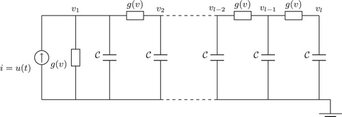
The first example is a nonlinear RC circuit [10] as shown in Figure 1. The nonlinearity is due to the nonlinear resistor with I–V characteristics given as $g\left(v\right)={\mathrm{e}}^{40v}+v-1$, where $g\left(v\right)$ is the current function and v is the voltage across the resistor. All the capacitances are fixed to $\mathcal{C}=1$. The nonlinearity in the RC circuit example can be transformed [14] to quadratic-bilinear form as in (1(1) $\begin{array}{rl}E\dot{x}\left(t\right)& =Ax\left(t\right)+Nx\left(t\right)u\left(t\right)+Qx\left(t\right)\otimes x\left(t\right)+Bu\left(t\right),\\ y\left(t\right)& =Cx\left(t\right),\end{array}$(1) ) by introducing some auxiliary variables. The transformation is exact, but the dimension of the system increases to $n=2\cdot l$, where l is the number of nodes in Figure 1, and is also the dimension of the original nonlinear system.

Figure 1. Nonlinear RC circuit.

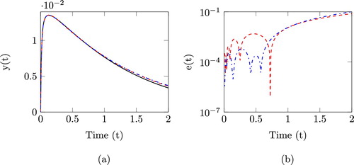
We fixed the number of nodes to l=500, so that the size of the quadratic-bilinear model (full order model (FOM)) is n=1000. We consider two cases for reduction of the FOM. In the first case, the size of the reduced quadratic-bilinear model is fixed to $r_1=r_2=6$ for both 2s-qbmor and m2s-qbmor. This means that for 2s-qbmor we compute three interpolation points using linear IRKA while for m2s-qbmor we use two interpolation points. Using an input $u\left(t\right)={\mathrm{e}}^{-t}$, where e represents the exponential function, the transient response of FOM and the two ROMs along with relative errors are shown in Figure 2. Notice that the reduced system obtained from the proposed m2s-qbmor has better transient response as compared to the one obtained from 2s-qbmor. The higher relative errors for larger t is because $y\left(t\right)\to 0$ as $t\to \mathrm{\infty }$.

Figure 2. Results for nonlinear RC circuit with $u\left(t\right)={\mathrm{e}}^{-t}$ and $s_1=3$, $s_2=2\text{ IRKA points}$; FOM of size n=1000 (

); ROM via 2s-qbmor of size $r_1=6$ (

) and ROM via m2s-qbmor of size $r_2=6$ (

): (a) transient response and (b) relative error $e\left(t\right)=\left(y\left(t\right)-\hat{y}\left(t\right)\right)/y\left(t\right)$.

The second case involves fixed interpolation points for both 2s-qbmor and m2s-qbmor. We used five interpolation points to obtain reduced systems of size $r_1=10$ via 2s-qbmor and $r_2=15$ using m2s-qbmor. Again with $u\left(t\right)={\mathrm{e}}^{-t}$, the transient responses and the relative errors for the same interpolation points are shown in Figure 3.

Figure 3. Results for nonlinear RC circuit with $u\left(t\right)={\mathrm{e}}^{-t}$ and $s_1=s_2=5\text{ IRKA points}$; FOM of size n=1000 (

); ROM via 2s-qbmor of size $r_1=10$ (

) and ROM via m2s-qbmor of size $r_2=15$ (

): (a) transient response and (b) relative error $e\left(t\right)=\left(y\left(t\right)-\hat{y}\left(t\right)\right)/y\left(t\right)$.

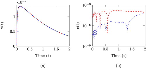
Although the two reduced systems are of different sizes, they are using the same interpolation points. The same number of interpolation points means the same number of sparse linear systems need to be solved, so the cost for constructing the reduced model is essentially the same. In that regard, it is a fair comparison regarding the efficiency of the offline phase. Clearly, for a given set of interpolation points, the proposed method computes more accurate reduced order models.

4.2. Burgers equation

As a second example, we consider the two-dimensional Burgers equation [6, 18]. The Burgers equation with domain, $\mathrm{\Gamma }=(0,1)\times (0,T)$ along with boundary conditions can be written as $\begin{array}{rl}& v_t+v{v}_x=\nu \cdot v_{xx},\text{in }\mathrm{\Gamma },\\ & \alpha v(0,t)+\beta x(0,t)=u\left(t\right),v_x(1,t)=0,t\in (0,T),\\ & v(x,0)=v_0\left(x\right),v_0\left(x\right)=0,x\in (0,1),\end{array}$ where ν is the viscosity and $v_0\left(x\right)$ is the initial condition. Semi-discretization of such partial differential equations naturally leads to a quadratic-bilinear system as given in (1(1) $\begin{array}{rl}E\dot{x}\left(t\right)& =Ax\left(t\right)+Nx\left(t\right)u\left(t\right)+Qx\left(t\right)\otimes x\left(t\right)+Bu\left(t\right),\\ y\left(t\right)& =Cx\left(t\right),\end{array}$(1) ). We set the state dimensions to n=1000 and compute reduced systems with both 2s-qbmor and m2s-qbmor having the same size, i.e. $r_1=r_2=6$, but different interpolation points (both using linear IRKA for interpolation points). The results are shown in Figure 4, for an input $u\left(t\right)=\cos \left(\pi t\right)$. 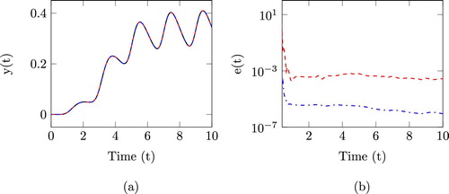Notice that even though the proposed method m2s-qbmor utilizes only two interpolation points, it still computes a reduced system with better accuracy as compared to 2s-qbmor where three interpolation points are used.

Figure 4. Results for Burgers equation with $u\left(t\right)=\cos \left(\pi t\right)$ and $s_1=3$, $s_2=2\text{ IRKA points}$; FOM of size n=1000 (

); ROM via 2s-qbmor of size $r_1=10$ (

) and ROM via m2s-qbmor of size $r_2=15$ (

): (a) transient response and (b) relative error  $e\left(t\right)=\left(y\left(t\right)-\hat{y}\left(t\right)\right)/y\left(t\right)$.

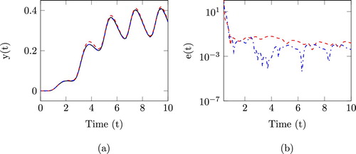
Next, we show the results for the same interpolation points. We compute five interpolation points using Linear IRKA and use these interpolation points to compute reduced systems of size 10 (via 2s-qbmor) and 15 (via m2s-qbmor). The transient responses of the actual and reduced systems along with their relative errors are shown in Figure 5. Clearly, the proposed method outperforms the standard two-sided projection method for a given set of interpolation points and as discussed in the first example, this comparison is fair because the cost for constructing the reduced model is essentially the same.

Figure 5. Nonlinear RC circuit with $u\left(t\right)=\cos \left(\pi t\right)$ and $s_1=s_2=5\text{ IRKA points}$; FOM of size n=1000 (

); ROM via 2s-qbmor of size $r_1=10$ (

) and ROM via m2s-qbmor of size $r_2=15$ (

): (a) transient response and (b) relative error  $e\left(t\right)=\left(y\left(t\right)-\hat{y}\left(t\right)\right)/y\left(t\right)$.

5. Conclusion

A modified sequence of projection matrices is identified in the two-sided projection technique for model reduction of quadratic-bilinear descriptor systems. The modified approach computes better reduced order models as compared to the existing two-sided projection techniques for a given set of interpolation points. An important future work would be to identify a sequence of projection matrices that can easily be extended to multi-input multi-output systems. Also, we would like to point out that despite the applicability of the proposed technique to descriptor systems (i.e. systems of the form (1) with E singular), we expect that some modifications of the method are necessary to achieve good approximation properties as in the linear [16] and bilinear [8] cases.

Disclosure statement

No potential conflict of interest was reported by the authors.

ORCID

Peter Benner http://orcid.org/0000-0003-3362-4103

Lihong Feng http://orcid.org/0000-0002-1885-3269

Additional information

Funding

Peter Benner is supported by the Deutsche Forschungsgemeinschaft (DFG, German Research Foundation) – 314838170, GRK 2297 MathCoRe.

References

- M. Ahmad, P. Benner and I. Jaimoukha, Krylov subspace methods for model reduction of quadratic-bilinear systems, IET Control Theory Appl. 10 (2016), pp. 2010–2018. doi: 10.1049/iet-cta.2016.0415
- A.C. Antoulas, Approximation of Large-Scale Dynamical Systems, SIAM Publications, Philadelphia, PA, 2005.
- A.C. Antoulas, D.C. Sorensen and S. Gugercin, A survey of model reduction methods for large-scale systems, Contemp. Math. 280 (2001), pp. 193–219. doi: 10.1090/conm/280/04630
- P. Benner and T. Breiten, Interpolation-based H2-model reduction of bilinear control systems, SIAM J. Matrix Anal. Appl. 33(3) (2012), pp. 859–885. doi: 10.1137/110836742
- P. Benner and T. Breiten, Two-sided moment matching methods for nonlinear model reduction, Tech. Rep. MPIMD/12-12, Max Planck Institute Magdeburg Preprints, Available at http://www.mpi-magdeburg.mpg.de/preprints/ (2012).
- P. Benner and T. Breiten, Two-sided projection methods for nonlinear model order reduction, SIAM J. Sci. Comput. 37(2) (2015), pp. B239–B260. doi: 10.1137/14097255X
- P. Benner, A. Cohen, M. Ohlberger and K. Willcox (Eds.), Model Reduction and Approximation: Theory and Algorithms, SIAM Publications, Philadelphia, PA, 2017.
- P. Benner and P. Goyal, Multipoint interpolation of Volterra series and H2-model reduction for a family of bilinear descriptor systems, Sys. Control Lett. 97 (2016), pp. 1–11. doi:10.1016/j.sysconle.2016.08.008.
- P. Benner, P. Goyal and S. Gugercin, H2-quasi-optimal model order reduction for quadratic-bilinear control systems, SIAM J. Matrix Anal. Appl. 39(2) (2018), pp. 983–1032. doi: 10.1137/16M1098280
- Y. Chen, Model reduction for nonlinear systems, Master's thesis, Massachusetts Institute of Technology (1999).
- G. Flagg and S. Gugercin, Multipoint Volterra series interpolation and H2 optimal model reduction of bilinear systems, SIAM J. Numer. Anal. 36(2) (2015), pp. 549–579. doi: 10.1137/130947830
- R.W. Freund, Model reduction methods based on Krylov subspaces, Acta Numer. 12 (2003), pp. 267–319. doi: 10.1017/S0962492902000120
- E.J. Grimme, Krylov projection methods for model reduction, PhD thesis, University of Illinois at Urbana-Champaign, USA (1997).
- C. Gu, QLMOR: a projection-based nonlinear model order reduction approach using quadratic-linear representation of nonlinear systems, IEEE Trans. Comput. Aided Des. Integr. Circuits Syst. 30(9) (2011), pp. 1307–1320. doi: 10.1109/TCAD.2011.2142184
- S. Gugercin, A.C. Antoulas and C. Beattie, H2 model reduction for large-scale dynamical systems, SIAM J. Matrix Anal. Appl. 30(2) (2008), pp. 609–638. doi: 10.1137/060666123
- S. Gugercin, T. Stykel and S. Wyatt, Model reduction of descriptor systems by interpolatory projection methods, SIAM J. Sci. Comput. 35(5) (2013), pp. B1010–B1033. doi:10.1137/130906635.
- T.G. Kolda and B.W. Bader, Tensor decompositions and applications, SIAM Rev. 51(3) (2009), pp. 455–475. doi: 10.1137/07070111X
- K. Kunisch and S. Volkwein, Proper orthogonal decomposition for optimality systems, ESAIM Math. Model. Numer. Anal. 42(1) (2008), pp. 1–23. doi: 10.1051/m2an:2007054
- R.J. Rugh, Nonlinear System Theory, Johns Hopkins University Press, Baltimore, MD, 1981.