
 ?Mathematical formulae have been encoded as MathML and are displayed in this HTML version using MathJax in order to improve their display. Uncheck the box to turn MathJax off. This feature requires Javascript. Click on a formula to zoom.
ABSTRACT
In the recent project BENCHOP – the BENCHmarking project in Option Pricing we found that Stochastic and Local Volatility problems were particularly challenging. Here we continue the effort by introducing a set of benchmark problems for this type of problems. Eight different methods targeted for the Stochastic Differential Equation (SDE) formulation and the Partial Differential Equation (PDE) formulation of the problem, as well as Fourier methods making use of the characteristic function, were implemented to solve these problems. Comparisons are made with respect to time to reach a certain error level in the computed solution for the different methods. The implemented Fourier method was superior to all others for the two problems where it was implemented. Generally, methods targeting the PDE formulation of the problem outperformed the methods for the SDE formulation. Among the methods for the PDE formulation the ADI method stood out as the best performing one.
1. Introduction
The aim of the original BENCHOP project described in [Citation34] was to provide researchers and practitioners in finance with a set of common benchmark problems for comparisons between methods and for evaluation of new methods. A wide range of existing numerical methods for each benchmark problem was implemented and the relative performance of the methods was compared. The problems were selected with respect to features that may be numerically challenging such as early exercise properties, barriers, discrete dividends, local volatility, stochastic volatility, jump diffusion, and two underlying assets.
In [Citation34] we found that stochastic and local volatility problems were particularly challenging. Hence, we here continue the effort to provide benchmark problems and performance comparisons between numerical methods at the research frontier for this type of problems. Stochastic and local volatility models provide an alternative approach to jump-diffusion models, and have proven effective in matching the rich asset price structure observed in derivatives markets. As is the case for jump-diffusion models, the market is typically incomplete in stochastic volatility models (in absence of assets that are directly traded on volatility risk), so additional assumptions are needed to uniquely determine asset prices. In [Citation19], for example, it is assumed that the volatility risk-premium is proportional to the volatility level.
We present the benchmark problems with sufficient detail so that others can solve them in the future. We also provide analytical solutions where such are available. Each problem is solved using MATLAB implementations of a number of numerical methods, and error plots as a function of computational time are provided. For details of the methods, we refer to the original papers, listed in Table . The codes are not fully optimized, and the numerical results should not be interpreted as competition scores. We rather see it as a general indication of their performance in terms of obtained accuracy versus computational time that could be expected in the computing environment under consideration. In order to facilitate future comparisons, MATLAB p-codes of the here presented methods for each benchmark problem will be made available through the BENCHOP web site http://www.it.uu.se/research/scientific_computing/project/compfin/benchop.
Table 1. List of methods used with abbreviations, marker symbol used in figures, references, and whether the MATLAB-implementation makes use of parallellism.
The paper is outlined as follows. In Section 2 we state the benchmark problems while the numerical methods are briefly presented in Section 3. Section 4 is dedicated to the presentation of the numerical results and finally in Section 5 we discuss the results. In Appendix 1 we present how the reference values are computed for the different problems. Finally, in Appendix 2 we specify the contributions from the authors of the paper.
2. Benchmark problems
2.1. Problem 1 – SABR stochastic-local volatility model
The Stochastic Alpha Beta Rho (SABR) model [Citation18] is an established Stochastic Differential Equation (SDE) system which is often used for interest rates and FX modelling in practice. A key feature of the model is that it matches the observed dynamic behaviour of the volatility smile, namely that when the price of the underlying decreases, the volatility smile shifts to lower prices, and vice versa. The SABR model is based on a parametric local volatility component in terms of a model parameter, β. The formal definition of the SABR model reads
where
denotes the forward value of the underlying asset
, with r the interest rate,
the spot price and T the contract's final time. The quantity
denotes the stochastic volatility,
and
are two correlated Brownian motions with constant correlation coefficient ρ (i.e.
). The free model parameters are
(the volatility of the volatility),
(the elasticity) and ρ (the correlation coefficient). The corresponding Partial Differential Equation (PDE) for the valuation of options is given by
for s>0,
and
.
Deliverables: The problem should be solved for a European call option with payoff at t=T, with three strikes
Parameter and problem specifications:
Set I ([Citation16]): T=2, r=0,
,
Set II ([Citation7]): T=10, r=0,
2.2. Problem 2 – quadratic local stochastic volatility model
The Quadratic Local Stochastic Volatility (QLSV) model, can be viewed as a generalization of Heston's stochastic volatility model [Citation19]. In the QLSV model, the square root term is multiplied by a quadratic function in the underlying asset. When the function is a constant, Heston's original model is obtained. The additional degrees of freedom provided by the quadratic function allows for improved volatility surface calibration.
We use the formulation in, e.g. [Citation26] and define the following SDE:
with
. The PDE for the valuation of options is then given by
for s>0, v>0 and
.
We consider a case when the Feller condition, is not satisfied (as is often the case in practice). The Feller condition [Citation9] ensures that the volatility process,
, remains strictly positive. If the condition is violated, the process may reach the boundary
. In this case, additional specification of the behaviour at the boundary is needed to ensure (weak) positivity, and the problem is also numerically more challenging (see [Citation8,Citation27]).
Deliverables: The problem should be solved for
a European call option with payoff
a Double-no-touch option paying 1 if
Parameter and problem specifications: We consider
a Heston model with
a QLSV model with
2.3. Problem 3 – Heston–Hull–White model
The Heston–Hull–White (HHW) model is a hybrid asset price model combining the Heston stochastic volatility model, and Hull–White stochastic interest rate model, see e.g. [Citation15,Citation17]. With such an approach the skew pattern for equity can be matched, while still allowing for stochastic interest rates. We define the HHW SDE:
and the corresponding HHW PDE:
for s>0, v>0, and
. Again, we will consider a case when the Feller condition is violated, see Section 2.2.
Deliverables: The problem should be solved for a European call option with payoff , K=100, and three spot values:
for
.
Parameter and problem specifications: We use the parameter set (cf. [Citation2,Citation17]):
3. Numerical methods
In Table we display all the methods that we have used. The methods are developed from the SDE or PDE formulation of the problem respectively, or make use of the characteristic function for the Fourier method. The methods are organized according to this in the table. To have a uniform presentation in Section 4 we use the same abbreviation and marker symbol for a given method in all figures in this section. Finally, Table provides references to the original papers describing the methods and also indicates whether the implementation is employing parallel constructions provided in Matlab Parallel Computing Toolbox or not. From the references in the table it should be clear which flavour of a method is actually used, when there are several similar approaches available.
It should be noted that even if a method is not parallelized here, it may still be parallelizable with good scalability.
4. Numerical results
In this section, we present the results using the different methods presented in Section 3 for the problems defined in Section 2. For all problems, we display errors in the computed solution as a function of wall clock time. The implementations were made in MATLAB and encrypted into p-code. The experiments were carried out at the Rackham Cluster at Uppsala Multidisciplinary Center for Advanced Computational Science at Uppsala University http://www.uppmax.uu.se/resources/systems/the-rackham-cluster/. The Rackham Cluster consists of 334 nodes where each node has two 10-core Intel Xeon V4 CPUs and at least 128 GB RAM memory. The experiments were performed on a dedicated node, i.e. using up to 20 MATLAB-workers. For the methods based on the SDE formulation of the problems, i.e. a Monte Carlo based solution method, the code was run three times and the mean of the results was reported. Finally, note that the axes in the figures are different for the different problems.
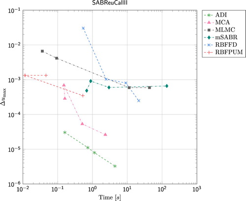
4.1. Results for SABR model
In Figures and we display the error
for the set of parameters (including
and
) defined in Section 2.1. Here u denotes the computed solution and
the reference solution, as a function of wall clock time for the SABR stochastic-local volatility model. Figure shows the results for Parameter Set I, and Figure the results for Parameter Set II. For both parameter sets, the ADI method is the most favourable one to use – for a given computational time the error is always smallest for this method. Among the Monte Carlo based methods, mSABR is the least favourable one to use for Parameter Set I while it is quite favourable to use for Parameter Set II if the required error in the solution is not too small (slightly less than
). For Parameter Set I MCA and MLMC behave similarly while MCA performs better than MLMC for Parameter Set II. For the RBF methods, RBFPUM performs better than RBFFD for relatively large errors (
). However, especially for Parameter Set I, RBFFD can provide smaller errors than RBFPUM does. For the SABR model, FGL was not implemented.
Figure 1. Results for the European call option under the SABR model, Parameter Set I. The reference values for ,
are given by 0.221383196830866, 0.193836689413803, and 0.166240814653231.
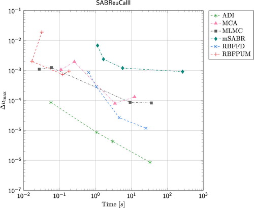
Figure 2. Results for the European call option under the SABR model, Parameter Set II. The reference values for ,
are given by 0.052450313614407, 0.046585753491306, and 0.039291470612989.
4.2. Results for QLSV model
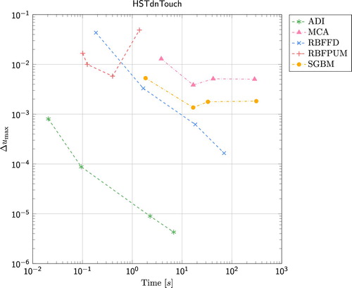
The error
(1)
(1) as a function of wall clock time for the European call option under the Heston model is presented in Figure , and the Double-no-touch option under the same model in Figure . Here we have used the set of parameters (including
and
) defined in Section 2.2. For the European call option, FGL outperforms all other methods. Already in less than 0.1 s, the error is below
for this method. The second best method is ADI which is also the method that is performing best for the Double-no-touch option. When it comes to the two RBF methods, RBFFD is the method of choice for this problem. For the European call option, the error for RBFPUM stays slightly below
and for the Double-no-touch option it stays around
. RBFFD on the other provides an error that is slightly larger than
in less than 100 s. The SGBM method is the best performing Monte Carlo type method for the Heston model. Both for the European option and the Double-no-touch option the time to reach a certain accuracy for SGBM is well below the time for MCA. Finally, for the European option, the performance of RBFFD and SGBM is similar, while RBFFD gives better results than SGBM for the Double-no-touch option.
Figure 3. Results for the European call option under the Heston model. The reference values for , 100, and 125 are given by 0.908502728459621, 9.046650119220969, and 28.514786399298796.
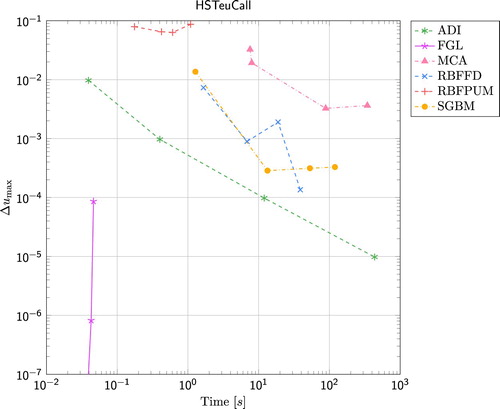
Figure 4. Results for the Double-no-touch option under the Heston model. The reference values for , 100, and 125 are given by 0.834539127387590, 0.899829293208866, and 0.668399975738358.
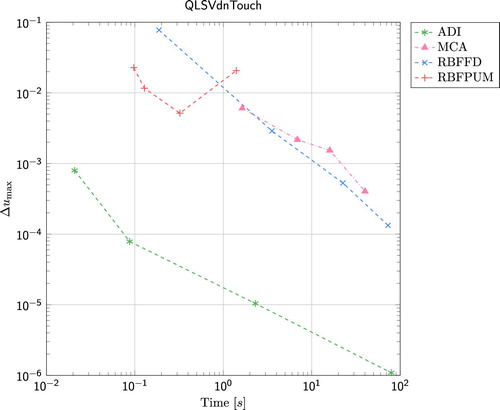
In Figures and the results for the European and Double-no-touch options under the QLSV model are presented. The Fourier method was not implemented for this model and the ADI method performed best for both types of options this time. To obtain low accuracy ( and
for European and Double-no-touch options respectively) the RBFPUM is the second best method that reaches these accuracies in less than 1 s. To obtain higher accuracy (
and
respectively) RBFFD is preferable between the two RBF methods. For the Double-no-touch option, MCA performs similarly as RBFFD while RBFFD outperforms MCA for the European call option.
Figure 5. Results for the European call option under the QLSV model. The reference values for , 100, and 125 are given by 0.527472759419533, 8.902347915743665, and 29.159828965633729.
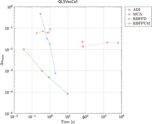
Figure 6. Results for the Double-no-touch option under the QLSV model. The reference values for , 100, and 125 are given by 0.933800903110254, 0.914799140676374, and 0.592983062889906.
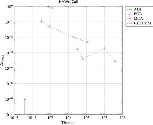
4.3. Results for HHW model
In Figure we present the results from the Heston–Hull–White model which is the only three-dimensional model among our benchmark problems. The error
(2)
(2) as a function of wall clock time is presented for the set of parameters (including
,
, and
) defined in Section 2.3. Again, FGL outperforms all other methods and reaches
in less than 0.1 s. ADI shows the same robust convergence behaviour as in the previous cases but this time MCA seems to perform equally well when considering accuracy versus computational time. It should be noted that the ADI code is a serial code while MCA is parallelized. Further, for MCA confidence intervals are not given. Finally, RBFPUM gives a fairly large error in this experiment.
Figure 7. Results for the European call option under the HHW model. The reference values for , 100, and 125 are given by 35.437896876285350, 54.728065308229503, and 75.397596834993621.
5. Discussion
In this paper, we have defined a set of benchmarking problems in option pricing for stochastic and local volatility problems. Eight different numerical methods have been implemented and compared with respect to error versus computational time.
The Fourier method FGL was implemented only for the European call option with the Heston model and the Heston–Hull–White model. In both cases, this method was superior to all others and reached extremely high accuracy with an error less than in less than 0.1 s. However, Fourier methods rely on the availability of the characteristic function of the underlying stochastic process or efficient approximations of the same.
For the problems when FGL was not implemented, the most efficient method was the ADI method. This was also together with RBFPUM and MCA the only method that was implemented for all problems. For the RBF methods, RBFPUM often reached a reasonable accuracy in a short time but had troubles with convergence with increasing computational time. RBFFD however, was in many cases the method that reached the smallest error after ADI (and FGL where applicable). The main challenge for the RBF methods was to apply appropriate boundary conditions in the volatility and interest rate dimensions. Some commonly used conditions introduced bias, while the option of leaving the boundary open in some cases lead to instability or inaccuracy.
For the methods based on the SDE formulation of the problems, it is difficult to draw any far-reaching conclusions. MLMC performed reasonably well for the SABR problems while mSABR gave reasonably small errors for Parameter Set II in a fairly short time. The mSABR method requires a smart application of a stochastic collocation-based method (see [Citation16]) to make the algorithm affordable in terms of computational time. Once the so-called integrated variance and volatility processes are simulated, the SABR forward asset process has been simulated by an extended Log-Euler discretization scheme, called Log-Euler+. MCA also gave quite accurate results in a reasonable time, especially for the SABR problems. For the Heston model (the special case of QLSV), SGBM was the best performing Monte Carlo type method. For the 3D problem Heston–Hull–White, MCA and ADI showed comparable results in this setting. This indicates as expected that Monte Carlo methods probably will be more competitive in higher dimensions.
Disclosure statement
No potential conflict of interest was reported by the authors.
Additional information
Funding
References
- M. Abramowitz and I.A. Stegun, Bessel functions J and Y, § 9.1 in Handbook of Mathematical Functions with Formulas, Graphs, and Mathematical Tables, Dover Publications, New York, NY, 10th printing, 1972.
- L. Andersen, Simple and efficient simulation of the Heston stochastic volatility model, J. Comput. Finance 11 (2008), pp. 1–42. doi: 10.21314/JCF.2008.189
- V. Bayona, N. Flyer, B. Fornberg, and G.A. Barnett, On the role of polynomials in RBF-FD approximations: II. numerical solution of elliptic PDEs, J. Comput. Phys. 332 (2017), pp. 257–273. doi: 10.1016/j.jcp.2016.12.008
- M. Broadie and Ö. Kaya, Exact simulation of stochastic volatility and other affine jump diffusion processes, Oper. Res. 54(2) (2006), pp. 217–231. doi: 10.1287/opre.1050.0247
- M. Brodén, J. Holst, E. Lindström, J. Ströjby, and M. Wiktorsson, Sequential calibration of options, Technical Report, Centre for Mathematical Sciences, Mathematical Statistics, Lund University, 2006. Contains additional material not included in the CSDA paper.
- P. Carr, H. Geman, D. Madan, L. Wu, and M. Yor, Option pricing using integral transforms, 2003. A slideshow presentation available at: http://www.math.nyu.edu/research/carrp/papers/pdf/integtransform.pdf.
- B. Chen, C.W. Oosterlee, and H. van der Weide, A low-bias simulation scheme for the SABR stochastic volatility model, Int. J. Theor. Appl. Finance 15(2) (2012), pp. 1250016-1–1250016-37. doi: 10.1142/S0219024912500161
- E. Ekström and J. Tysk, Boundary conditions for the single-factor term structure equation, Ann. Appl. Probab. 21(1) (2011), pp. 332–350. doi: 10.1214/10-AAP698
- W. Feller, Two singular diffusion problems, Ann. Math. 54 (1951), pp. 173–182. doi: 10.2307/1969318
- Q. Feng and C. Oosterlee, Monte Carlo calculation of exposure profiles and Greeks for Bermudan and barrier options under the Heston Hull–White model, in Recent Progress and Modern Challenges in Applied Mathematics, R. Melnik, R. Makarov, and J. Belair, eds., Springer Fields Institute Communications, 2017, pp. 265–301.
- N. Flyer, B. Fornberg, V. Bayona, and G.A. Barnett, On the role of polynomials in RBF–FD approximations: I. Interpolation and accuracy, J. Comput. Phys. 321 (2016), pp. 21–38. doi: 10.1016/j.jcp.2016.05.026
- M.B. Giles, Multilevel Monte Carlo path simulation, Oper. Res. 56(3) (2008), pp. 607–617. doi: 10.1287/opre.1070.0496
- G.H. Givens and J.A. Hoeting, Computational Statistics, Vol. 710. John Wiley & Sons, Hoboken, NJ, 2012.
- G.H. Golub and J.H. Welsch, Calculation of Gauss quadrature rules, Math. Comput. 23(106) (1969), pp. 221–230. doi: 10.1090/S0025-5718-69-99647-1
- L.A. Grzelak and C.W. Oosterlee, On the Heston model with stochastic interest rates, SIAM J. Financial Math. 2 (2011), pp. 255–286. doi: 10.1137/090756119
- L.A. Grzelak, J.A.S. Witteveen, M. Suárez-Taboada, and C.W. Oosterlee, The stochastic collocation Monte Carlo sampler: Highly efficient sampling from “expensive” distributions, Quant. Finance (2018). doi:10.1080/14697688.2018.1459807.
- T. Haentjens and K.J. In 't Hout, Alternating direction implicit finite difference schemes for the Heston–Hull–White partial differential equation, J. Comput. Finance 16 (2012), pp. 83–110. doi: 10.21314/JCF.2012.244
- P.S. Hagan, D. Kumar, A.S. Lesniewski, and D.E. Woodward, Managing smile risk, Wilmott Mag. 1 (2002), pp. 84–108.
- S.L. Heston, A closed-form solution for options with stochastic volatility with applications to bond and currency options, Rev. Financial Stud. 11 (1993), pp. 327–343. doi: 10.1093/rfs/6.2.327
- K.J. In 't Hout and S. Foulon, ADI finite difference schemes for option pricing in the Heston model with correlation, Int. J. Numer. Anal. Model. 7(2) (2010), pp. 303–320.
- K.J. In 't Hout and B.D. Welfert, Unconditional stability of second-order ADI schemes applied to multi-dimensional diffusion equations with mixed derivative terms, Appl. Numer. Math. 59(3–4) (2009), pp. 677–692. doi: 10.1016/j.apnum.2008.03.016
- S. Jain and C.W. Oosterlee, The stochastic grid bundling method: Efficient pricing of Bermudan options and their Greeks, Appl. Math. Comput. 269 (2015), pp. 412–431.
- R.W. Lee, Option pricing by transform methods: Extensions, unification and error control, J. Comput. Finance 7(3) (2004), pp. 51–86. doi: 10.21314/JCF.2004.121
- A. Leitao, L.A. Grzelak, and C.W. Oosterlee, On an efficient multiple time step Monte Carlo simulation of the SABR model, Quant. Finance 17(10) (2017), pp. 1549–1565. URL https://doi.org/10.1080/14697688.2017.1301676.
- E. Lindström, J. Ströjby, M. Brodén, M. Wiktorsson, and J. Holst, Sequential calibration of options, Comput. Stat. Data Anal. 52(6) (2008), pp. 2877–2891. doi: 10.1016/j.csda.2007.08.009
- A. Lipton, A. Gal, and A. Lasis, Pricing of vanilla and first-generation exotic options in the local stochastic volatility framework: Survey and new results, Quant. Finance 14 (2014), pp. 1899–1922. doi: 10.1080/14697688.2014.930965
- V. Lucic, Boundary conditions for computing densities in hybrid models via PDE methods, Stoch. Int. J. Probab. Stoch. Process. 84(5–6) (2012), pp. 705–718. doi: 10.1080/17442508.2012.656270
- S. Milovanović and V. Shcherbakov, Pricing derivatives under multiple stochastic factors by localized radial basis function methods. arXiv:1711.09852 [q-fin.CP], 2017.
- S. Milovanović and L. von Sydow, Radial basis function generated finite differences for option pricing problems, Comput. Math. Appl. 75(4) (2018), pp. 1462–1481. doi: 10.1016/j.camwa.2017.11.015
- K.-S. Moon, Efficient Monte Carlo algorithm for pricing barrier options, Commun. Korean Math. Soc. 23(2) (2008), pp. 285–294. doi: 10.4134/CKMS.2008.23.2.285
- A. Safdari-Vaighani, A. Heryudono, and E. Larsson, A radial basis function partition of unity collocation method for convection–diffusion equations arising in financial applications, J. Sci. Comput. 64 (2014), pp. 1–27.
- V. Shcherbakov, Radial basis function partition of unity operator splitting method for pricing multi-asset American options, BIT Numer. Math. 56 (2016), pp. 1401–1423. doi: 10.1007/s10543-016-0616-y
- V. Shcherbakov and E. Larsson, Radial basis function partition of unity methods for pricing vanilla basket options, Comput. Math. Appl. 71 (2016), pp. 185–200. doi: 10.1016/j.camwa.2015.11.007
- L. von Sydow, L.J. Höök, E. Larsson, E. Lindström, S. Milovanović, J. Persson, V. Shcherbakov, Y. Shpolyanskiy, S. Sirén, J. Toivanen, and J. Waldén, BENCHOP – the BENCHmarking project in Option Pricing, Int. J. Comput. Math. 92(12) (2015), pp. 2361–2379. doi: 10.1080/00207160.2015.1072172
- M. Wiktorsson, Pricing using Fourier based methods applied to the SABR model in the case of zero correlation, 2018. Working paper available at: http://www.maths.lth.se/matstat/staff/magnusw/papers/SABR_notes.pdf.
- M. Wyns and K.J. In 't Hout, An adjoint method for the exact calibration of stochastic local volatility models, J. Comput. Sci. 24 (2018), pp. 182–194. doi: 10.1016/j.jocs.2017.02.004
Appendices
Appendix 1. The methods used for computing the reference values used in the comparisons
When there is no analytical formula available we have used the ADI method with a very small tolerance to compute the reference values. The estimated error in these values is computed as the absolute difference between two subsequent solutions in a refinement sequence of ADI solutions. As with all numerical methods, there could be some bias in this.
A.1. Methods for problem 1 – SABR
Case I: To our knowledge, no analytical formula allowing for highly accurate evaluation of the European call option under the SABR model was previously available in the literature. For the parameters we use in Case I, with uncorrelated Brownian motions for the stock and
for the volatility, a new price formula has been derived. The full details of the derivations are found in [Citation35]. If we denote the European call option price at time t for the SABR model with strike K and maturity T by
, we have that
where the probabilities
and
are expressed through the following integrals:
where
and the variable
, which is associated with the integration path of an inverse Laplace transform, should be chosen such that
where
We calculate these integrals using Gauss–Hermite quadrature points for x and Gauss–Laguerre quadrature points for Using 2000 points in the x and
direction, i.e. a total of 4 million points we get the values.
Table A1. SABR European call prices using the parameters from case I. Error .
Case II: The solution was obtained by an ADI method since the analytical method only works in the zero correlation case. The ADI method employed spatial grid points and 445 time steps.
Table A2. SABR European call prices using the parameters from case II. Error .
A.2. Methods for problem 2 – QSLV
Heston European call: The solution was obtained using a Fourier–Gauss–Laguerre implementation with 1000 quadrature points.
Table A3. Heston European call prices. Error .
Heston Double-no-touch: The solution was obtained by an ADI method since analytical methods only work in the European case. The ADI method employed spatial grid points and 757 time steps.
Table A4. Heston Double-no-touch prices with lower barrier L=50 and upper barrier U=150. Error .
QSLV European call: The solution was obtained by an ADI method since analytical methods only work in the zero correlation case. The ADI method employed spatial gridpoints and 743 time steps.
Table A5. Case quadratic stochastic-Local-Volatility European call prices. Error .
QSLV Double-no-touch: The solution was obtained by an ADI method using spatial grid points and 1060 time steps.
Table A6. quadratic stochastic-Local-Volatility Double-no-touch prices with lower barrier L=50 and upper barrier U=150. Error .
A.3. Methods for problem 3 – HHW
The solution was computed using a Fourier–Gauss–Laguerre implementation with 1000 quadrature points.
Table A7. Heston European call prices. Error .
Appendix 2. The contribution from the authors
Apart from what is listed in Table all authors took part in reading and correcting of the final version of the paper.
Table A8. Name and contribution of authors.
During the time for the project, three meetings were held:
A kick-off meeting in Uppsala in August 2016, dedicated for the set-up of the project.
An intermediate planning meeting in Austin in connection with the SIAM Conference on Financial Mathematics & Engineering in November 2016.
A final planning meeting in Leiden in connection with the Lorentz center workshop in Applied Mathematics Techniques for Energy Markets in Transition in September 2017.
In Table it is presented at what meetings the authors took part.