Numerical simulations in 3-dimensions of reaction–diffusion models for brain tumour growth

ABSTRACT

We work with a well-known model of reaction–diffusion type for brain tumour growth and accomplish full 3-dimensional (3d) simulations of the tumour in time on two types of imaging data, the 3d Shepp–Logan head phantom image and an MRI T1-weighted brain scan from the Internet Brain Segmentation Repository. The source term is such that we have logistic growth. These simulations are obtained using standard finite difference approximations with novel calculations to increase speed and accuracy. Moreover, biological background to the model, its well-posedness together with a variational formulation are given. The variational formulation enable the feasibility of different derivations and modifications of the model.

KEYWORDS:

• Nonlinear parabolic equations
• reaction–diffusion equations
• 3-dimensional simulations of brain tumour growth
• mathematical biology
• medical imaging

2010 MATHEMATICS SUBJECT CLASSIFICATIONS:

• 35Q92
• 35Kxx
• 65N06

1. Introduction

Brain cancer is a common cancer worldwide; in 2012 it was the 17th one with nearly 256 thousand new cases contributing to about $1.83\mathrm{\%}$ of the total number of new cancer cases diagnosed [14]. Typical treatment involves surgery, radiotherapy and chemotherapy but even with all the therapeutic progress, brain tumours are still rarely completely curable. A helpful tool for comprehending cancer progression is to apply mathematical models and simulations to predict the evolution of the disease. Standard models for brain tumour growth are built on partial differential equations of reaction–diffusion type. These models describe the evolution of the tumour cell density and its interaction with the underlying visible tissue structures like the grey matter, white matter and bones. An important advantage of these models is that they can be validated in time using real patient data such as a sequence of MRI images.

Cancer research is extending rapidly and constantly more complex models are designed for better determining the growth of tumours. For beginners in the field it can be helpful to see simulations of standard basic models to understand their performance and drawbacks. To the authors knowledge, only two-dimensional simulations seem presented in the literature for the basic reaction–diffusion models for tumour growth. Since the models are inevitably nonlinear the simplification to 2-dimensions could render different and spurious behaviour. Thus, in the present work, we undertake the laborious task of doing full 3-dimensional simulations for two cases: The standard 3-dimensional Shepp–Logan phantom [42] and an MRI T1-weighted brain scan [40] from the Internet Brain Segmentation Repository (IBSR) (see [20]) describing a more complex geometry. We aim to not use any commercial solvers for partial differential equations but show instead how a rather straightforward finite difference scheme can be employed combined with recent imaging techniques [1] to render the simulations. We also show how existence and uniqueness of a solution to the reaction–diffusion model can be obtained using basic concepts of weak formulations. It is then natural to also present a variational formulation that can aid in deriving and modifying the reaction–diffusion model.

The presented numerical simulations building on [1] with biological and mathematical background to the model are the main novelties of the present work. Since modelling of tumours involves both medical and mathematical insights it is believed that collecting such in one work with full simulations will be useful for interdisciplinary teams where participants typically have either a strong medical or mathematical background but not both. Thus, having a brief overview containing both medical and mathematical aspects can help in quickly bridging the gap between clinicians and mathematicians.

For the outline, in Section 2, we present some background on the biological context and imaging for brain tumours. In Section 3, we expound highlighted studies on various types of brain tumour growth models based on reaction–diffusion equations according to brain structure using data imaging. Sections 2 and 3 are extracted from our work presented in [21]. Section 4 is devoted to mathematical analysis of reaction–diffusion equations and their well-posedness. In Section 5, we introduce a variational formulation of the problem. In Section 6, for completeness, we give details of the numerical implementation; the similar scheme is presented in our paper [23] for an inverse problem. Additionally, we show in this section results of numerical simulations of the growth of two types of tumours using full 3-dimensional imaging data. Finally, some conclusions are given in Section 7.

2. Background on brain tumours

2.1. Biological context

A tumour is an abnormal growth of normal tissue cells due to genetic and epigenetic events. After the tumour grows to a certain size, it starts to actively infiltrate healthy tissue. This invasion is one of the hallmarks of cancer, as described by Hanahan and Weinberg [18]. It is often the final step of a malignant tumour and leads to metastasis and to eventual death of the patient.

Brain tumour cells are widely known to be highly diffusive and infiltrating compared with other types of tumours. They consist of motile cells and are not nearly as dense as others. These cells go out of the original tumour mass, move extremely quickly and wander far away from the tumour centre via natural pathways of higher diffusivity, such as brain white matter fiber tracts. Consequently, the tumour mass has no well-defined edges and it fills up space within the cranial cavity. It can compress, shift, invade and damage healthy brain tissue thereby interfering with normal brain functions causing clinical symptoms such as headache, seizures, neurological and cognitive deficits.

Brain tumours are classified based on their origin into primary brain tumours that start in the brain and remain there, and metastatic brain tumours that have spread to the brain from another location in the body. Gliomas are a type of brain tumour that make up about $30\mathrm{\%}$ of all primary and metastatic brain tumours and about $80\mathrm{\%}$ of all malignant brain tumours [17]. The classification is as Grade I through Grade IV according to the World Health Organization (WHO) grading system [32] based on how aggressive the tumour cells of the biopsied tissue appear under a microscope.

Low-Grade Gliomas (LGG) include grade I (astroglial variants that can be cured with complete surgical resection) and grade II (diffusively infiltrating LGG that make surgery difficult with high probability of recurrences: astrocytomas, oligodendrogliomas and mixed gliomas). They are slow growing tumours that look almost normal and infiltrate into normal brain ground tissue. Their progression to a high-grade glioma is almost inevitable [27].

High-Grade Gliomas (HGG) include grade III (Anaplastic astrocytomas) and grade IV (Glioblastomas Multiforma GBM). They look abnormal and are characterized by rapid proliferation, infiltration into large areas. They might also have a necrotic core, form new vascularization to support growth and push the surrounding tissue causing a mass-effect [11].

The median survival time is 7.5 years for LGG (grade II) and 18 months for astrocytomas (grade III) with treatments. For GBM, it is 17 weeks without treatment, 30 weeks with radiotherapy and 37 weeks with both surgical resection and radiotherapy.

Besides grading, staging is used to communicate whether and where a tumour has spread in the brain. Staging is typically inferred based on morphological assessment using imaging techniques like Computed Tomography (CT) and Magnetic Resonance Imaging (MRI) [13].

2.2. Imaging

The most common MRI sequences include T1 and T2 weighted images. Gadolinium contrast agent can be administered to the patient in order to acquire T1 with contrast agent weighted images (T1Gd). T2 weighted FLAIR images (T2-FLAIR) stands for Fluid Attenuation Inversion Recovery T2 images. It is similar to T2 images but with a better contrast due to the attenuation of the signal coming from the cerebro-spinal fluid (CSF). These sequences are preferably performed in at least 2-orthogonal planes or obtained with a 3-dimensional (3D) sequence that is reformatted into orthogonal planes (i.e. 3D-T2 FLAIR) [33].

The usual delineated structures of the tumour are the necrotic core, the proliferative rim and the edema. The necrotic core and the proliferative rim are visible on the T1Gd MRI. On the T2 FLAIR, one can delineate the edema of the tumour.

Diffusion Weighted Imaging (DWI) uses the diffusion of water molecules in tissues to generate contrast in MR images and can be used to calculate the Average Diffusion Coefficient (ADC). A special kind of DWI, Diffusion-tensor imaging (DTI), has been used extensively to map white matter tractography in the brain. It involves more directions of interrogation than standard DWI but provides additional parameters and abilities over DWI. DTI provides information on anisotropic diffusion characterized by eigenvectors (direction) and eigenvalues (magnitude), which can be used to derive numerous parameters. The Fractional Anisotropy (FA) derived from DTI is a measure of the directional nature of water diffusivity. It is often anti-correlated to the ADC: high ADC values result in low FA values.

Although MR is the main diagnostic tool for diseases of the central nervous system, Computational Tomography (CT) is still a valuable modality in the imaging of brain tumours (CT involves X-rays which MR does not). CT is superior in detecting calcification, hemorrhage, and in evaluating bone changes related to a tumour [12].

Finally, advanced imaging techniques can also be used such as perfusion images which reveal tumour and tissue vascularity and MR spectroscopy which reveals the tumour metabolic profile.

3. Background on brain tumour growth models

The choice of a model is largely guided by the available data. In fact, observations at the microscopic (histological) scale are used to design very detailed mathematical tumour growth models [34]. These proposed theoretical models take the form of ordinary differential equations (ODEs) involving only the density of cells in the tumour: $\frac{\mathrm{d}u}{\mathrm{d}t}=f\left(u\right),$ where $u\left(t\right)>0$ is the tumour cells density at time t and $f\in C^1$ is a function describing the cells proliferation rate through general frameworks for tumour growth kinetics. Its expression is given by the generalized logistic equation: $f\left(u\right)=\rho u^{\alpha }\beta (1-u^{1/\beta }{)}^{\gamma },$ where α, β, γ are non-negative real numbers and $\beta >0$.

Standard models for the growth of brain tumours are classified according to the function f and include: (1) $f\left(u\right)=\left\{\begin{array}{ll}\rho u& \alpha =1,\beta =1,\gamma =0\mathrm{Exponential},\\ \rho u(1-u)& \alpha =1,\beta =1,\gamma =1\mathrm{Logistic},\\ -\rho u\ln \left(u\right)& \alpha =1,\beta \to +\mathrm{\infty },\gamma =1\mathrm{Gompertz},\end{array}\right.$(1) where $\rho >0$ is the proliferation rate.

The simplest growth assumes a linear relationship of the tumour cell density, resulting in exponential growth stating that cellular division obeys a cycle, with doubling time $\ln \left(2\right)/\rho$. This renders a biologically accurate description of tumour growth on time scales that are short in comparison to the life expectancy after the initial tumour development [4]. The logistic and gompertz type growth functions are considered to encapsulate the effect of a maximal capacity of tumour cells incorporating cell population decay with respect to a given carrying capacity.

Such models give a better understanding of cancer initiation and progression by describing the tumour growth process at the cellular level and its interaction with the micro-environment (e.g. in [2] Basanta et al. used evolutionary game theory to build a model that allows to understand certain specific aspects of glioma progression such as the emergence of diffusive tumour cell invasion in Low-Grade tumours and in [26] Kansal et al. developed a three-dimensional cellular automaton model of brain tumour Gompertzian growth). However, these models do not take into account the spatial arrangement of the cells at a specific location or the spatial spread of the cancerous cells.

Partial differential equations (PDEs) are suited to describe the space and time evolution of cell densities. They are in fact the tool of choice when studying tumour growth and diffusion into surrounding tissue. An early study by Cruywagen et al. [10] proposed to use a reaction–diffusion framework for modelling the dynamics of a human brain tumour (HGG). In that study they consider the evolution of the brain tumour cell population to be largely governed by proliferation and diffusion. This basic model was formulated by Murray in [36] as a conservation equation. Letting $u(x,t)$ be the cells density at a position x (pixel or voxel location in the brain) and at a time t, the governing model is: $\frac{\mathrm{\partial }u}{\mathrm{\partial }t}=\text{div}\left(\mathbf{J}\right)+f\left(u\right),$ where $\text{div}$ is the divergence operator and $\mathbf{J}$ is the diffusional flux of cells taken according to Fick's law as proportional to the gradient of the cell density, that is $\mathbf{J}=D\mathrm{\nabla }u$, with ∇ the gradient operator and D the diffusion coefficient of cells in the brain tissue.

Boundary conditions are imposed to prevent cells from leaving the finite space domain (the skull), with a point-source initial condition of the cell density $\varphi \left(x\right)=u(x,0)$ simulating the start of a tumour. The general form of the model is then given by: (2) $\begin{array}{rl}{\mathrm{\partial }}_{t}u-\text{div}\left(D\mathrm{\nabla }u\right)-f\left(u\right)& =0\text{in}\mathrm{\Omega }\times (0,T)\\ u\left(0\right)& =\varphi \text{in}\mathrm{\Omega }\\ D\mathrm{\nabla }u\cdot n& =0\text{on}\mathrm{\partial \Omega }\times (0,T),\end{array}$(2) where Ω is the brain region inside the skull and n the outward unit normal vector to the boundary $\mathrm{\partial \Omega }$.

In early works, the proliferation of tumour cells was assumed to be exponential $f\left(u\right)=\rho u$ and the diffusion tensor D isotropic in a homogeneous brain structure Ω: $D=dI,$ where I is the identity matrix and d>0 a constant value for the diffusion coefficient. This kind of tensor allow tumour cells to diffuse equally in all directions and all across the brain.

Murray [35], related the velocity v of the tumour growth to the proliferation rate ρ and the diffusion coefficient d such that $v=2\sqrt{\rho d}$. This work lead the way to studies by Tracqui [45] that gave rise to the first approximations of model parameters d and ρ using CT scans for HGG.

The effect of therapy has been included in this model using an additional term describing the death of tumour cells due to therapy (e.g. Cruywagen et al. modelled the effects of chemotherapy on two subpopulations of HGG cells resistent and sensitive [10] and Woodward et al. focused on the resection effect on LGG and HGG in [46]).

An extension of the model to 3-dimensions has been done by Burgess et al. in [5] for LGG and HGG.

In later studies, reaction–diffusion models have been used to describe HGG growth in the heterogeneous environment of the brain. In [43], Swanson et al. take into account the brain tissue heterogeneity assuming that the tumour cells proliferation was also exponential and the diffusion tensor D of equation (1) was isotropic but spatially dependent: $D=d\left(x\right)I,$ where I is the identity matrix and the diffusion coefficient is $d\left(x\right)=\left\{\begin{array}{ll}{d}_g& \text{in grey brain tissue},\\ d_w& \text{in white brain tissue},\end{array}\right.$ where $d_w>>d_g>0$ corresponding to the observation that tumour cells move faster on white matter [16].

Swanson et al. [44] extended the model to 3-dimensions taking advantage of the information about white and grey matter areas extracted from the BrainWeb anatomical atlas [8,9]. They showed how the model parameters could be estimated using only in vivo post-contrast T1 weighted and T2 weighted MRI data.

While the grey matter is mostly homogeneous, tumour cells are known to use the fibrous structures of the white matter to invade new areas. Moreover, observations showed that tumour cells tend to follow the preferred directions of water diffusion, which can be measured using magnetic resonance diffusion tensor imaging (MR-DTI). In this context, refining on the differential motility of tumour cells in different tissues, many authors constructed inhomogeneous diffusion tensors D to model the diffusion of tumour cells from the Diffusion Tensor Images (DTI): $D=\mathbf{\text{D(x)}}.$ The tensor construction method consisted of using isotropic (spherical) tensors in grey matter and anisotropic (ellipsoid) diffusion in white matter.

Using a 3d segmented MRI atlas, Clatz et al. [7] proposed a model coupling between reaction diffusion and the mechanical constitutive equations to simulate the mass effect (brain deformation induced by the tumour invasion) during GBMs growth. In the reaction diffusion equations, they used exponential growth for the tumour cells proliferation to simplify the model and assumed that in white matter the anisotropic diffusion ratio is the same for water molecules and tumour cells: $\mathbf{\text{D(x)}}=\left\{\begin{array}{ll}{d}_g\mathbf{\text{I}}& \text{in grey matter},\\ d_w{\mathbf{\text{D}}}_{\mathbf{\text{water}}}& \text{in white matter},\end{array}\right.$ where ${\mathbf{D}}_{\mathbf{w}\mathbf{a}\mathbf{t}\mathbf{e}\mathbf{r}}$ is the water diffusion tensor in the brain measured by the DTI, i.e. the spatial diffusion of water molecules by MRI per voxel. It contains the full diffusion information along six directions.

To increase the tensor anisotropy in white matter without changing its orientation and also favouring the appropriate orientations when fiber crossing occurs, in their proposed LGG growth model [24] Jbabdi et al. have introduced a formulation which takes into account the possible equality of the two largest eigenvalues corresponding to a possible fiber crossing keeping exponential growth for proliferation and isotropic diffusion in grey matter: $\mathbf{\text{D(x)}}=\left\{\begin{array}{ll}{d}_g\mathbf{\text{I}}& \text{in grey matter},\\ \mathbf{\text{V(x)}}\left[\mathrm{diag}\right(\alpha e_1\left(x\right)d_w,d_g,d_g\left)\right]{\mathbf{\text{V(x)}}}^T& \text{in white matter},\end{array}\right.$ where $\mathbf{V}\mathbf{\left(}\mathbf{x}\mathbf{\right)}$ represents the matrix of sorted eigenvectors obtained by decomposing ${\mathbf{D}}_{\mathbf{w}\mathbf{a}\mathbf{t}\mathbf{e}\mathbf{r}}\mathbf{\left(}\mathbf{x}\mathbf{\right)}$; $e_1\left(x\right)$ is the normalized largest eigenvalue (between 0 and 1) of ${\mathbf{D}}_{\mathbf{w}\mathbf{a}\mathbf{t}\mathbf{e}\mathbf{r}}\mathbf{\left(}\mathbf{x}\mathbf{\right)}$ and α is a normalization factor such that the highest $e_1$ value in the brain becomes 1. In this framework, the LGG growth model is directly applied to the extracted tensors without any additional registration.

Finally, let us mention that besides the prediction of brain tumour growth some authors [15,19,22,28,39] have recently used these image-based reaction–diffusion models for source localization.

4. Reaction–diffusion models

In the remaining part of this work, we denote for simplicity $D\left(x\right)$ by D. We shall investigate existence and uniqueness of a solution to (3) $\begin{array}{rl}{\mathrm{\partial }}_{t}u-\text{div}\left(D\mathrm{\nabla }u\right)-f\left(u\right)& =0\text{ in }\mathrm{\Omega }\times (0,T)\\ D\mathrm{\nabla }u\cdot n& =0\text{on}\mathrm{\partial \Omega }\times (0,T)\\ u(x,0)& =\varphi \text{ in }\mathrm{\Omega }.\end{array}$(3) We first introduce some function spaces. The space $L^2(0,T;X)$, where X is a Hilbert space, consists of those measurable functions $u(\cdot ,t):(0,T)\to X$, with ${\int }_0^T\parallel u(\cdot ,t){\parallel }_X^2\mathrm{d}t<\mathrm{\infty }.$ By $C^k\left(\right[0,T];X)$, we denote the functions u for which the mapping $u(\cdot ,t):[0,T]\to X$ have continuous and bounded (in the usual norm) derivatives of order up to $k\ge 0$. The space $H^k\left(\mathrm{\Omega }\right)$, k>0, is the standard Sobolev space of functions with weak and square integrable derivatives up to order k, with trace space $H^{k-1/2}\left(\mathrm{\Gamma }\right)$.

Concerning the existence and uniqueness of a solution to (3(3) $\begin{array}{rl}{\mathrm{\partial }}_{t}u-\text{div}\left(D\mathrm{\nabla }u\right)-f\left(u\right)& =0\text{ in }\mathrm{\Omega }\times (0,T)\\ D\mathrm{\nabla }u\cdot n& =0\text{on}\mathrm{\partial \Omega }\times (0,T)\\ u(x,0)& =\varphi \text{ in }\mathrm{\Omega }.\end{array}$(3) ), there are several different options to prove this. On an abstract level, the problem can be recast as $\begin{array}{rl}{u}_t^{\prime }+Bu& =f\left(u\right(t\left)\right)\\ u\left(0\right)& =\varphi \end{array}$ making it essentially an ODE in the time-variable but with values in a function space. Here, B corresponds to the divergence term, and generates a semi-group S, see [38, Theorem 7.2.5]. Existence and uniqueness of what is known as a mild solution, $u\left(t\right)=S\left(t\right)\varphi +{\int }_0^{t}S(t-s)f\left(u\right(s\left)\right)\mathrm{d}s$ is given by [38, Theorem 6.1.2] (in the space $C(0,T;H^1(\mathrm{\Omega }\left)\right)$). However, this abstract machinery takes some effort to get into and since we have tumour growth in mind, we also outline a second route to show existence and uniqueness which is more direct and can be useful from a computational side.

Multiplying (3(3) $\begin{array}{rl}{\mathrm{\partial }}_{t}u-\text{div}\left(D\mathrm{\nabla }u\right)-f\left(u\right)& =0\text{ in }\mathrm{\Omega }\times (0,T)\\ D\mathrm{\nabla }u\cdot n& =0\text{on}\mathrm{\partial \Omega }\times (0,T)\\ u(x,0)& =\varphi \text{ in }\mathrm{\Omega }.\end{array}$(3) ) by an element $v\in H^1\left(\mathrm{\Omega }\right)$ and using integration by parts in the space variables (a Green formula), incorporating the zero flux condition on the boundary, give (4) ${\int }_{\mathrm{\Omega }}{u}_t^{\prime }(x,\cdot )v\left(x\right)\mathrm{d}x+{\int }_{\mathrm{\Omega }}D\mathrm{\nabla }u(x,\cdot )\cdot \mathrm{\nabla }v\left(x\right)\mathrm{d}x={\int }_{\mathrm{\Omega }}f\left(u\right(x,\cdot \left)\right)v\left(x\right)\mathrm{d}x.$(4) An element u is termed a weak solution to (3(3) $\begin{array}{rl}{\mathrm{\partial }}_{t}u-\text{div}\left(D\mathrm{\nabla }u\right)-f\left(u\right)& =0\text{ in }\mathrm{\Omega }\times (0,T)\\ D\mathrm{\nabla }u\cdot n& =0\text{on}\mathrm{\partial \Omega }\times (0,T)\\ u(x,0)& =\varphi \text{ in }\mathrm{\Omega }.\end{array}$(3) ) provided that (4(4) ${\int }_{\mathrm{\Omega }}{u}_t^{\prime }(x,\cdot )v\left(x\right)\mathrm{d}x+{\int }_{\mathrm{\Omega }}D\mathrm{\nabla }u(x,\cdot )\cdot \mathrm{\nabla }v\left(x\right)\mathrm{d}x={\int }_{\mathrm{\Omega }}f\left(u\right(x,\cdot \left)\right)v\left(x\right)\mathrm{d}x.$(4) ) holds and $u(x,0)=\varphi$.

To approximate the time-derivative in (3(3) $\begin{array}{rl}{\mathrm{\partial }}_{t}u-\text{div}\left(D\mathrm{\nabla }u\right)-f\left(u\right)& =0\text{ in }\mathrm{\Omega }\times (0,T)\\ D\mathrm{\nabla }u\cdot n& =0\text{on}\mathrm{\partial \Omega }\times (0,T)\\ u(x,0)& =\varphi \text{ in }\mathrm{\Omega }.\end{array}$(3) ), we apply the backward difference $u_t^{\prime }(x,t_k)=\frac{u_k\left(x\right)-u_{k-1}\left(x\right)}{\tau },$ where $t_k=\left(T/N\right)k$, $k=0,1,\dots ,N$, is a uniform mesh on the time interval $[0,T]$ with step size $\tau =T/N$, and $u_k\left(x\right)=u(x,t_k)$.

Employing this time-discretization in (4(4) ${\int }_{\mathrm{\Omega }}{u}_t^{\prime }(x,\cdot )v\left(x\right)\mathrm{d}x+{\int }_{\mathrm{\Omega }}D\mathrm{\nabla }u(x,\cdot )\cdot \mathrm{\nabla }v\left(x\right)\mathrm{d}x={\int }_{\mathrm{\Omega }}f\left(u\right(x,\cdot \left)\right)v\left(x\right)\mathrm{d}x.$(4) ) together with evaluating the nonlinear term at the previous mesh point, we derive the identity (5) ${\int }_{\mathrm{\Omega }}\frac{u_k\left(x\right)-u_{k-1}\left(x\right)}{\tau }v\left(x\right)\mathrm{d}x+{\int }_{\mathrm{\Omega }}D\mathrm{\nabla }{u}_k\left(x\right)\cdot \mathrm{\nabla }v\left(x\right)\mathrm{d}x={\int }_{\mathrm{\Omega }}f\left(u_{k-1}\right(x\left)\right)v\left(x\right)\mathrm{d}x,$(5) or by rewriting this, (6) $\frac{1}{\tau }{\int }_{\mathrm{\Omega }}{u}_k\left(x\right)v\left(x\right)\mathrm{d}x+{\int }_{\mathrm{\Omega }}D\mathrm{\nabla }{u}_k\left(x\right)\cdot \mathrm{\nabla }v\left(x\right)\mathrm{d}x={\int }_{\mathrm{\Omega }}\left(f\left(u_{k-1}\right(x\left)\right)+\frac{u_{k-1}\left(x\right)}{\tau }\right)v\left(x\right)\mathrm{d}x.$(6) This is then a standard linear elliptic problem for $u_k$ (for k=0 the condition $u(x,0)=\varphi$ is used). Existence and uniqueness of $u_k\in H^1\left(\mathrm{\Omega }\right)$ is settled via the Lax–Milgram lemma, see [6, Chapter 1]. Note that this holds for any of the different tensors D described in the previous sections, in fact a piecewise continuous tensor can be used.

The sequence of functions $\left\{u_k\right\}$ can then be interpolated into a time-dependent approximation simplest by defining this to be piecewise constant at each interval $[t_{k-1},t_k)$, alternatively to be linear at each such interval. This is known as the Rothe approximation. It is then possible to show that, as the step size τ decreases, the interpolated function tends to a solution of (4(4) ${\int }_{\mathrm{\Omega }}{u}_t^{\prime }(x,\cdot )v\left(x\right)\mathrm{d}x+{\int }_{\mathrm{\Omega }}D\mathrm{\nabla }u(x,\cdot )\cdot \mathrm{\nabla }v\left(x\right)\mathrm{d}x={\int }_{\mathrm{\Omega }}f\left(u\right(x,\cdot \left)\right)v\left(x\right)\mathrm{d}x.$(4) ) in the appropriate norms. In this way, existence of a weak solution can be shown. For the linear case, an introduction to the method of Rothe is given in [25, Chapter 1].

For the uniqueness, assume that there are two weak solutions u and $\tilde{u}$ to (3(3) $\begin{array}{rl}{\mathrm{\partial }}_{t}u-\text{div}\left(D\mathrm{\nabla }u\right)-f\left(u\right)& =0\text{ in }\mathrm{\Omega }\times (0,T)\\ D\mathrm{\nabla }u\cdot n& =0\text{on}\mathrm{\partial \Omega }\times (0,T)\\ u(x,0)& =\varphi \text{ in }\mathrm{\Omega }.\end{array}$(3) ). Put $w=u-\tilde{u}$, then w satisfies a relation of the form (4(4) ${\int }_{\mathrm{\Omega }}{u}_t^{\prime }(x,\cdot )v\left(x\right)\mathrm{d}x+{\int }_{\mathrm{\Omega }}D\mathrm{\nabla }u(x,\cdot )\cdot \mathrm{\nabla }v\left(x\right)\mathrm{d}x={\int }_{\mathrm{\Omega }}f\left(u\right(x,\cdot \left)\right)v\left(x\right)\mathrm{d}x.$(4) ) with $f\left(u\right)$ in the right-hand side replaced by $f\left(u\right)-f\left(\tilde{u}\right)$ and $\varphi =0$. Note that (4(4) ${\int }_{\mathrm{\Omega }}{u}_t^{\prime }(x,\cdot )v\left(x\right)\mathrm{d}x+{\int }_{\mathrm{\Omega }}D\mathrm{\nabla }u(x,\cdot )\cdot \mathrm{\nabla }v\left(x\right)\mathrm{d}x={\int }_{\mathrm{\Omega }}f\left(u\right(x,\cdot \left)\right)v\left(x\right)\mathrm{d}x.$(4) ) can be extended to hold for v, which are piecewise constant in time, and by a limiting argument this relation holds for all $v(x,t)\in L^2(0,T;H^1(\mathrm{\Omega }\left)\right)$. Hence, choosing v=w in the weak relation for w, we have (7) ${\int }_{\mathrm{\Omega }}{w}_t^{\prime }(x,\cdot )w(x,\cdot )\mathrm{d}x+{\int }_{\mathrm{\Omega }}D\mathrm{\nabla }w(x,\cdot )\cdot \mathrm{\nabla }w(x,\cdot )\mathrm{d}x={\int }_{\mathrm{\Omega }}\left(f\right(u(x,\cdot ))-f(\tilde{u}(x,\cdot )\left)\right)w\left(x\right)\mathrm{d}x.$(7) Integrating in time over $[0,t]$ in the first term noting that ${\mathrm{\partial }}_t{w}^2=2w^{\prime }w$ and estimating the second term in the left-hand side of (7(7) ${\int }_{\mathrm{\Omega }}{w}_t^{\prime }(x,\cdot )w(x,\cdot )\mathrm{d}x+{\int }_{\mathrm{\Omega }}D\mathrm{\nabla }w(x,\cdot )\cdot \mathrm{\nabla }w(x,\cdot )\mathrm{d}x={\int }_{\mathrm{\Omega }}\left(f\right(u(x,\cdot ))-f(\tilde{u}(x,\cdot )\left)\right)w\left(x\right)\mathrm{d}x.$(7) ) from below, we obtain (8) $\parallel w(x,t){\parallel }_{L^2\left(\mathrm{\Omega }\right)}^2+\parallel \mathrm{\nabla }w{\parallel }_{L^2\left(Q_t\right)}^2\le C{\int }_0^t{\int }_{\mathrm{\Omega }}\left(f\right(u(x,\cdot ))-f(\tilde{u}(x,\cdot )\left)\right)w\left(x\right)\mathrm{d}x\mathrm{d}t.$(8) The function f is assumed to be Lipschitz continuous, hence we can further estimate using this and Cauchy's inequality, (9) $\parallel w(x,\cdot ){\parallel }_{L^2\left(\mathrm{\Omega }\right)}^2+\parallel \mathrm{\nabla }w{\parallel }_{L^2\left(Q_t\right)}^2\le C\parallel w{\parallel }_{L^2\left(Q_t\right)}^2.$(9) According to a version of Grönwall's lemma, see [41, p. 25], this implies that the left-hand side is zero, which in turn, since t with 0<t<T was arbitrary, forces w=0 in $Q_T$ and we have uniqueness.

The above steps albeit on a more general level is performed in [41, Chapter 8], where the reader can find full details on the above arguments, which renders the following result ([41, Theorem 8.33 and Proposition 8.37]).

Theorem 4.1

Let $\varphi \in L^2\left(\mathrm{\Omega }\right)$. Then there exists a unique weak solution $u\in L^2(0,T;H^1(\mathrm{\Omega }\left)\right)$ with $u_t^{\prime }\in L^2(0,T;L^2(\mathrm{\Omega }\left)\right)$ to the reaction–diffusion problem (3(3) $\begin{array}{rl}{\mathrm{\partial }}_{t}u-\text{div}\left(D\mathrm{\nabla }u\right)-f\left(u\right)& =0\text{ in }\mathrm{\Omega }\times (0,T)\\ D\mathrm{\nabla }u\cdot n& =0\text{on}\mathrm{\partial \Omega }\times (0,T)\\ u(x,0)& =\varphi \text{ in }\mathrm{\Omega }.\end{array}$(3) ), and this element u depends continuously on the data.

It is possible to give an interpretation of the Neumann condition for a weak solution, see [30, Chapter 4.7.2, Example 2], and one can prove a similar result for a weak solution with a non-homogeneous Neumann condition. Regularity of the weak solution can also be shown, in fact, existence and uniqueness for classical solutions in spaces of Hölder continuous and differentiable functions have been derived, see [29, p. 491, Theorem 7.4].

There is also another concept of a solution to (3(3) $\begin{array}{rl}{\mathrm{\partial }}_{t}u-\text{div}\left(D\mathrm{\nabla }u\right)-f\left(u\right)& =0\text{ in }\mathrm{\Omega }\times (0,T)\\ D\mathrm{\nabla }u\cdot n& =0\text{on}\mathrm{\partial \Omega }\times (0,T)\\ u(x,0)& =\varphi \text{ in }\mathrm{\Omega }.\end{array}$(3) ), which is usually termed a very weak solution. In this formulation, one multiplies $\left(1\right)$3(3) $\begin{array}{rl}{\mathrm{\partial }}_{t}u-\text{div}\left(D\mathrm{\nabla }u\right)-f\left(u\right)& =0\text{ in }\mathrm{\Omega }\times (0,T)\\ D\mathrm{\nabla }u\cdot n& =0\text{on}\mathrm{\partial \Omega }\times (0,T)\\ u(x,0)& =\varphi \text{ in }\mathrm{\Omega }.\end{array}$(3) with a function $v(x,t)$ and integrates over both time and space to have a relation ${\int }_{Q_T}u{v}_t^{\prime }\mathrm{d}x\mathrm{d}t+{\int }_{Q_T}D\mathrm{\nabla }u\cdot \mathrm{\nabla }u=-{\int }_{Q_T}f\left(u\right)v\mathrm{d}x\mathrm{d}t+{\int }_{\mathrm{\Omega }}\varphi v(x,0)\mathrm{d}x,$ for $v\in L^2(0,T;H^1(\mathrm{\Omega }\left)\right)\cap H^1(0,T;L^2(\mathrm{\Omega }\left)\right)$ with $v(T,x)=0$. Thus, no derivative in time is directly imposed on u in this formulation. One can show existence and uniqueness of a very weak solution as well [41, Chapter 8.7] (for an application, the concept of a very weak solution was used in [3] to reconstruct boundary data for the heat equation). The reader can verify that a mild solution is a very weak solution as is a weak solution. We also point out that spaces of the form $L^2(0,T;H^k(\mathrm{\Omega }\left)\right)\cap H^s(0,T;L^2(\mathrm{\Omega }\left)\right)$ is sometimes denoted $H^{k,s}\left(Q_T\right)$; for properties and trace theorems, see [31, Chapter 2].

5. Variational formulation

Variational formulations can be useful in designing mathematical models. Moreover, variational formulations have been pivotal for image enhancement methods. In this section, we briefly show how to generate a more general brain tumour growth model by finding a functional E such that the stationary form of the reaction–diffusion equation (2(2) $\begin{array}{rl}{\mathrm{\partial }}_{t}u-\text{div}\left(D\mathrm{\nabla }u\right)-f\left(u\right)& =0\text{in}\mathrm{\Omega }\times (0,T)\\ u\left(0\right)& =\varphi \text{in}\mathrm{\Omega }\\ D\mathrm{\nabla }u\cdot n& =0\text{on}\mathrm{\partial \Omega }\times (0,T),\end{array}$(2) ) is the Euler–Lagrange (E–L) equation corresponding to E. This means that the stationary points of the functional satisfies Equation (2(2) $\begin{array}{rl}{\mathrm{\partial }}_{t}u-\text{div}\left(D\mathrm{\nabla }u\right)-f\left(u\right)& =0\text{in}\mathrm{\Omega }\times (0,T)\\ u\left(0\right)& =\varphi \text{in}\mathrm{\Omega }\\ D\mathrm{\nabla }u\cdot n& =0\text{on}\mathrm{\partial \Omega }\times (0,T),\end{array}$(2) ). Mathematically, we have the following result, where F is convex and D is positive definite:

If $f\left(u\right)$ is the Gâteaux derivative of $F\left(u\right)$ with respect to u, then $E\left(u\right)=\frac{1}{2}{\int }_{\mathrm{\Omega }}(u-u^0{)}^2\mathrm{d}x+\frac{\lambda }{2}{\int }_{\mathrm{\Omega }}|D\mathrm{\nabla }u{|}^2\mathrm{d}x+\lambda {\int }_{\mathrm{\Omega }}F(u)\mathrm{d}x$ is the functional which corresponds to the E–L equation (2(2) $\begin{array}{rl}{\mathrm{\partial }}_{t}u-\text{div}\left(D\mathrm{\nabla }u\right)-f\left(u\right)& =0\text{in}\mathrm{\Omega }\times (0,T)\\ u\left(0\right)& =\varphi \text{in}\mathrm{\Omega }\\ D\mathrm{\nabla }u\cdot n& =0\text{on}\mathrm{\partial \Omega }\times (0,T),\end{array}$(2) ).

To verify this, we have to calculate the (Gâteaux) derivative of $E\left(u\right)$ to find its stationary points. We start by finding the derivative of the second term of E.

Let $R\left(u\right)=\frac{1}{2}{\int }_{\mathrm{\Omega }}|D\mathrm{\nabla }u{|}^2\mathrm{d}x.$ Let then $v\in C^1\left(\mathrm{\Omega }\right)$ be an arbitrary function not equal to zero ($v\ne 0$), we compute the Gâteaux derivative as follows: $\begin{array}{rl}{\mathrm{\partial }}_{u}R\left(u\right)v& =\underset{ϵ\to 0}{lim}\frac{1}{2ϵ}{\int }_{\mathrm{\Omega }}\left(|D\mathrm{\nabla }\right(u+ϵv){|}^2-|D\mathrm{\nabla }u{|}^2)\mathrm{d}x\\ & =\underset{ϵ\to 0}{lim}\frac{1}{2ϵ}{\int }_{\mathrm{\Omega }}(|D\mathrm{\nabla }u{|}^2+2ϵ(D\mathrm{\nabla }u{)}^{t}D\mathrm{\nabla }v+{ϵ}^2|D\mathrm{\nabla }v{|}^2-|D\mathrm{\nabla }u{|}^2)\mathrm{d}x\\ & ={\int }_{\mathrm{\Omega }}(D\mathrm{\nabla }u{)}^{t}D\mathrm{\nabla }v\mathrm{d}x\end{array}$ and by applying Green's first identity, the above expression results in ${\int }_{\mathrm{\Omega }}(D\mathrm{\nabla }u{)}^{t}D\mathrm{\nabla }v\mathrm{d}x={\int }_{\mathrm{\partial \Omega }}Dv(D\mathrm{\nabla }u\cdot n)dS-{\int }_{\mathrm{\Omega }}Dv\text{div}(D\mathrm{\nabla }u)\mathrm{d}x.$ Using the Neumann boundary condition $D\mathrm{\nabla }u\cdot n=0$, the previous equation reads ${\mathrm{\partial }}_{u}R\left(u\right)v=-{\int }_{\mathrm{\Omega }}Dv\text{div}\left(D\mathrm{\nabla }u\right)\mathrm{d}x.$ For the derivation of the Gâteaux derivative of the first and second term of E, let $S\left(u\right)=-{\int }_{\mathrm{\Omega }}F\left(u\right)\mathrm{d}x.$ Then let $v\in C^1\left(\mathrm{\Omega }\right)$ be an arbitrary function not equal to zero ($v\ne 0$), we compute the Gâteaux derivative as follows: $\begin{array}{rl}{\mathrm{\partial }}_{u}S\left(u\right)v& =\underset{ϵ\to 0}{lim}-{\int }_{\mathrm{\Omega }}\frac{F(u+ϵv)-F\left(u\right)}{ϵ}\mathrm{d}x\\ & =-{\int }_{\mathrm{\Omega }}\frac{\mathrm{\partial }}{\mathrm{\partial }ϵ}F(u+ϵv){|}_{ϵ=0}\mathrm{d}x\\ & =-{\int }_{\mathrm{\Omega }}{F}^{\prime }(u+ϵv)v{|}_{ϵ=0}\mathrm{d}x.\end{array}$ It follows that ${\mathrm{\partial }}_{u}S\left(u\right)v=-{\int }_{\mathrm{\Omega }}{F}^{\prime }\left(u\right)v\mathrm{d}x.$ Thus, with this expression we can find the derivative of both the first and second term of E (by choosing F appropriately).

Since $v\ne 0$ and D has non-zero elements $d_{ii}\ne 0$, the E–L equation is therefore (10) $\begin{array}{rl}u-u^0-\text{div}\left(D\mathrm{\nabla }u\right)-f\left(u\right)& =0\text{in }\mathrm{\Omega }\times (0,T)\\ u\left(0\right)& =\varphi \text{in }\mathrm{\Omega }\\ D\mathrm{\nabla }u\cdot n& =0\text{on }\mathrm{\partial \Omega }\times (0,T),\end{array}$(10) where (11) $F^{\prime }\left(u\right)=f\left(u\right).$(11) One can then introduce what is known as artificial time marching, where a problem of the form (2(2) $\begin{array}{rl}{\mathrm{\partial }}_{t}u-\text{div}\left(D\mathrm{\nabla }u\right)-f\left(u\right)& =0\text{in}\mathrm{\Omega }\times (0,T)\\ u\left(0\right)& =\varphi \text{in}\mathrm{\Omega }\\ D\mathrm{\nabla }u\cdot n& =0\text{on}\mathrm{\partial \Omega }\times (0,T),\end{array}$(2) ) is solved to steady-state using explicit time-stepping, the steady state then being (10(10) $\begin{array}{rl}u-u^0-\text{div}\left(D\mathrm{\nabla }u\right)-f\left(u\right)& =0\text{in }\mathrm{\Omega }\times (0,T)\\ u\left(0\right)& =\varphi \text{in }\mathrm{\Omega }\\ D\mathrm{\nabla }u\cdot n& =0\text{on }\mathrm{\partial \Omega }\times (0,T),\end{array}$(10) ).

For the sake of completeness, we give the corresponding functions F for the standard terms f of (11(11) $F^{\prime }\left(u\right)=f\left(u\right).$(11) ):

• $f\left(u\right)=\rho u$⇒$F\left(u\right)=\rho u^2/2+C$

• $f\left(u\right)=\rho u(1-u)$⇒$F\left(u\right)=\rho (u^2/2-u^3/3)+C$

• $f\left(u\right)=-\rho u\ln \left(u\right)$⇒$F\left(u\right)=-\rho (u^2/2\ln (u)-u^2/4)+C$.

The constant C should be chosen such that F is non-negative. In this general context, f and F model respectively a local and a total proliferation of the tumour cells. Let us mention that, if we define F as the entropy of the system $F\left(u\right)=-\rho \ln \left(u\right)$, then a better choice of the local proliferation function f will be a mixed model of exponential and gompertz models: $f\left(u\right)=\rho u-\rho u\ln \left(u\right)$.

6. Numerical simulations

In the numerical experiments, we consider the test case of isotropic diffusion with logistic growth in a heterogeneous domain: (12) $\begin{array}{rl}{\mathrm{\partial }}_{t}u-\text{div}\left(D\mathrm{\nabla }u\right)-\rho u(1-u)& =0\text{ in }\mathrm{\Omega }\times (0,T)\\ D\mathrm{\nabla }u\cdot n& =0\text{ on }\mathrm{\partial \Omega }\times (0,T)\\ u(x,0)& =\varphi \text{ in }\mathrm{\Omega },\end{array}$(12) where $0\le u(x,t)\le 1$ is the normalized tumour cell density, Ω is the domain representing the brain and $\begin{array}{r}D\left(x\right)=\left\{\begin{array}{c}{d}_{w}I,\text{ in white matter},\\ d_{g}I,\text{ in gray matter},\end{array}\right.\end{array}$ where I is the $3\times 3$ identity matrix and ρ, $d_w$ and $d_g$ are positive constants. Letting ${\mathrm{\Omega }}_w$ and ${\mathrm{\Omega }}_g$ be the regions of white matter and the grey matter in the brain, respectively, we can write the tensor $D\left(x\right)$ as (13) $D\left(x\right)=a\left(x\right)d_{w}I+b\left(x\right)d_{g}I,$(13) where $\begin{array}{r}a\left(x\right)=\left\{\begin{array}{c}1,x\in {\mathrm{\Omega }}_w\\ 0,x\notin {\mathrm{\Omega }}_w\end{array}\right.\text{and}b\left(x\right)=\left\{\begin{array}{c}1,x\in {\mathrm{\Omega }}_g,\\ 0,x\notin {\mathrm{\Omega }}_g.\end{array}\right.\end{array}$ 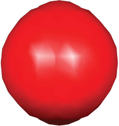The initial tumour cell density, shown in Figure 1, is assumed to be a three-dimensional Gaussian distribution: $u(x,0)=\varphi =\frac{1}{\sqrt{\left|\mathrm{\Sigma }\right|(2\pi {)}^3}}\exp \left(-\frac{1}{2}{x}^{\prime }{\mathrm{\Sigma }}^{-1}x\right)$ with a diagonal covariance matrix $\mathrm{\Sigma }=1.3I$ (leading to a product of three independent Gaussian distributions), where the mean is zero and $|\cdot |$ is the determinant. In the code developed for the simulations, one can replace this initial distribution with another function, however, we only present result for this ϕ since it is standard in tumour modelling to have Gaussian initial distributions.

Figure 1. Initial tumour cell density $u(x,0)=\varphi$.

6.1. Data

We use two types of three-dimensional ($3d$) imaging data. The first setting is the standard 3d Shepp–Logan phantom [42] describing a simple geometry, and the second setting is an MRI T1-weighted brain scan [40] from the IBSR [20] describing a more complex geometry.

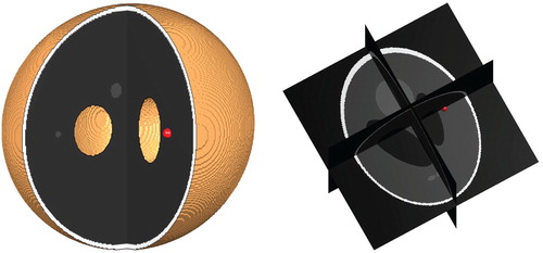
In the synthetic setting of the 3d Shepp–Logan phantom, we manually selected hypothetical white and gray matter regions as shown in Figure 2. Unlike in the 3d Shepp–Logan image, the MRI data image has ground truth segmentation of white and gray matter regions provided by experts, see Figure 3 for illustration of these regions. In these two figures, the regions are shown on three different and orthogonal planes (slices) through the brain; the planes used are as is illustrated for example in the last image in Figure 4.

Figure 2. Hypothetical segmentation of Ω in the $3d$ Shepp–Logan image.

Figure 3. Ground truth segmentation of Ω in the MRI T1 image.

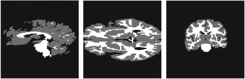
Figure 4. Position of the initial tumour cell density in the 3d Shepp–Logan image and its corresponding 3d planes.

The domain Ω represents the brain region (the union of the grey and white matter). In the computations this corresponds to the 3-dimensional images representing the brain: In the Shepp–Logan image, the total number of voxels is $256\times 256\times 256$, thus Ω is a cube. For the MR1 T1-weighted brain scan, the total number of voxels is $256\times 256\times 46$, hence Ω is here a cuboid. The region outside the skull is empty and only introduced for convenience as is common in finite difference methods.

6.2. Parameters

Table 1 shows the values chosen for the model parameters, that is values for the proliferation rate ρ and diffusion rates $d_w$ and $d_g$ for Low Grade Glioma (LGG) and High Grade Glioma (HGG). The variation of the parameter ρ influences the degree of the nonlinearity for the logistic source term, see (1(1) $f\left(u\right)=\left\{\begin{array}{ll}\rho u& \alpha =1,\beta =1,\gamma =0\mathrm{Exponential},\\ \rho u(1-u)& \alpha =1,\beta =1,\gamma =1\mathrm{Logistic},\\ -\rho u\ln \left(u\right)& \alpha =1,\beta \to +\mathrm{\infty },\gamma =1\mathrm{Gompertz},\end{array}\right.$(1) ), in the PDE model (12(12) $\begin{array}{rl}{\mathrm{\partial }}_{t}u-\text{div}\left(D\mathrm{\nabla }u\right)-\rho u(1-u)& =0\text{ in }\mathrm{\Omega }\times (0,T)\\ D\mathrm{\nabla }u\cdot n& =0\text{ on }\mathrm{\partial \Omega }\times (0,T)\\ u(x,0)& =\varphi \text{ in }\mathrm{\Omega },\end{array}$(12) ).

Table 1. Parameters values for Low Grade Glioma (LGG) and High Grade Glioma (HGG).

	LGG	HGG
ρ	0.012	0.009
$d_w$	0.25	0.5
$d_g$	0.01	0.25

6.3. Discretization

For numerical implementation of the reaction–diffusion model, we consider an evolution equation of the form: ${\mathrm{\partial }}_{t}u=Au+f\left(u\right),$ where A is a spatially dependent linear differential operator containing derivatives on its diagonal. The following explicit iterative discretization scheme is used in time due to its simplicity: $u^{i+1}=u^i+hA{u}^i+hf\left(u^i\right),$ where $i=0,1,\dots$, is the current iteration, h>0 is the stepsize and the matrix A, also known as the stencil, can be expressed via a sparse representation making memory requirements less demanding.

We then also need to approximate the spatial derivatives present in A. We adopt a generic forward Euler discretization strategy using finite differences approximating derivatives in parabolic PDEs [37]. Expanding the divergence term, we have: (14) $\text{div}\left(D\mathrm{\nabla }u\right)=\text{div}\left[\begin{array}{c}\left(\begin{array}{c}{d}_{11}00\\ 0d_{22}0\\ 00d_{33}\end{array}\right)\left(\begin{array}{c}{\mathrm{\partial }}_{x}u\\ {\mathrm{\partial }}_{y}u\\ {\mathrm{\partial }}_{z}u\end{array}\right)\end{array}\right]={\mathrm{\partial }}_x\left(d_{11}{\mathrm{\partial }}_{x}u\right)+{\mathrm{\partial }}_y\left(d_{22}{\mathrm{\partial }}_{y}u\right)+{\mathrm{\partial }}_z\left(d_{33}{\mathrm{\partial }}_{z}u\right),$(14) where the indices of d are the corresponding components in terms of rows and columns of D. We point out that the elements of D are dependent on space as given in (13(13) $D\left(x\right)=a\left(x\right)d_{w}I+b\left(x\right)d_{g}I,$(13) ).

The terms in (14(14) $\text{div}\left(D\mathrm{\nabla }u\right)=\text{div}\left[\begin{array}{c}\left(\begin{array}{c}{d}_{11}00\\ 0d_{22}0\\ 00d_{33}\end{array}\right)\left(\begin{array}{c}{\mathrm{\partial }}_{x}u\\ {\mathrm{\partial }}_{y}u\\ {\mathrm{\partial }}_{z}u\end{array}\right)\end{array}\right]={\mathrm{\partial }}_x\left(d_{11}{\mathrm{\partial }}_{x}u\right)+{\mathrm{\partial }}_y\left(d_{22}{\mathrm{\partial }}_{y}u\right)+{\mathrm{\partial }}_z\left(d_{33}{\mathrm{\partial }}_{z}u\right),$(14) ) involve derivatives up to second order. We approximate these derivatives by averaging the forward, ${\mathrm{\partial }}^{+}$, and backward, ${\mathrm{\partial }}^{-}$, finite difference operators using the following alternating scheme of forward and backward differences for the x -, y- and z -directions: (15) $\begin{array}{r}{\mathrm{\partial }}_x\left(d_{11}{\mathrm{\partial }}_{x}u\right)\approx \frac{1}{2}\left({\mathrm{\partial }}_x^{+}\right(d_{11}{\mathrm{\partial }}_x^{-}u)+{\mathrm{\partial }}_x^{-}(d_{11}{\mathrm{\partial }}_x^{+}u\left)\right)\\ {\mathrm{\partial }}_y\left(d_{22}{\mathrm{\partial }}_{y}u\right)\approx \frac{1}{2}\left({\mathrm{\partial }}_y^{+}\right(d_{22}{\mathrm{\partial }}_y^{-}u)+{\mathrm{\partial }}_y^{-}(d_{22}{\mathrm{\partial }}_y^{+}u\left)\right)\\ {\mathrm{\partial }}_z\left(d_{11}{\mathrm{\partial }}_{z}u\right)\approx \frac{1}{2}\left({\mathrm{\partial }}_z^{+}\right(d_{33}{\mathrm{\partial }}_z^{-}u)+{\mathrm{\partial }}_z^{-}(d_{33}{\mathrm{\partial }}_z^{+}u\left)\right).\end{array}$(15) Letting the size of one voxel be 1 (other sizes can easily be adjusted for) given in each of the three directions, we derive the forward ${\mathrm{\partial }}^{+}$ and backward ${\mathrm{\partial }}^{-}$ finite difference operators as second-order approximations from a third-order Taylor series expansion in the respective direction: $\begin{array}{r}\begin{array}{c}{\mathrm{\partial }}_x^{+}u=u(x+1,y,z)-u(x,y,z)\\ {\mathrm{\partial }}_x^{-}u=u(x,y,z)-u(x-1,y,z)\end{array}\begin{array}{c}{\mathrm{\partial }}_y^{+}u=u(x,y+1,z)-u(x,y,z)\\ {\mathrm{\partial }}_y^{-}u=u(x,y,z)-u(x,y-1,z)\end{array}\end{array}$ $\begin{array}{r}\begin{array}{c}{\mathrm{\partial }}_z^{+}u=u(x,y,z+1)-u(x,y,z)\\ {\mathrm{\partial }}_z^{-}u=u(x,y,z)-u(x,y,z-1)\end{array}\end{array}$ From this, we get the approximations: (16) $\begin{array}{r}{\mathrm{\partial }}_x\left(d_{11}{\mathrm{\partial }}_{x}u\right)\approx \frac{1}{2}\left[\right(d_{11}(x+1,y,z)+d_{11}(x,y,z)\left)\right(u(x+1,y,z)-u(x,y,z))-\\ \left(d_{11}\right(x-1,y,z)+d_{11}(x,y,z\left)\right)\left(u\right(x,y,z)-u(x-1,y,z\left)\right)]\\ {\mathrm{\partial }}_y\left(d_{22}{\mathrm{\partial }}_{y}u\right)\approx \frac{1}{2}\left[\right(d_{22}(x,y+1,z)+d_{22}(x,y,z)\left)\right(u(x,y+1,z)-u(x,y,z))-\\ \left(d_{22}\right(x,y-1,z)+d_{22}(x,y,z\left)\right)\left(u\right(x,y,z)-u(x,y-1,z\left)\right)]\\ {\mathrm{\partial }}_z\left(d_{33}{\mathrm{\partial }}_{z}u\right)\approx \frac{1}{2}\left[\right(d_{33}(x,y,z+1)+d_{33}(x,y,z)\left)\right(u(x,y,z+1)-u(x,y,z))-\\ \left(d_{33}\right(x,y,z-1)+d_{33}(x,y,z\left)\right)\left(u\right(x,y,z)-u(x,y,z-1\left)\right)].\end{array}$(16) Since the boundary of Ω is the (curved) boundary of the brain (union of white and gray matter segments), special care is needed when computing the Neumann boundary condition on irregular grids. We approach this problem by sequentially replicating the boundary voxels in the outward normal direction of Ω. Any inconsistency for diagonal flow vectors have not been observed in the simulations, in fact this straightforward strategy performs remarkably well.

6.4. Setup

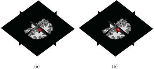
We run the model to obtain a synthetic tumour at a time T>0 for the two different parameter configurations (LGG, respectively, HGG) given in Table  1. Figures 4 and 5 show the initial setup of the tumour cell density for the Shepp–Logan image and the MRI T1 data, respectively.

Figure 5. Position of the initial tumour cell density in the MRI T1 image and its corresponding 3d planes.

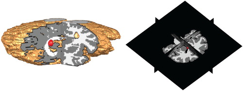
To aid the visualization, we created a numerical routine to render the corresponding 3d planes. In those illustrations, it is in general easier to see the position and growth of the tumour.

In all the presented experiments, the time-step in the Euler scheme is 0.1. Other time-steps have been tested and the approach seem stable with respect to this parameter. The problem is iterated over time to illustrate the growth of LGG and HGG tumour types as well as to illustrate the behaviour of the tumour near the boundaries of the brain.

6.5. Results

Figures 6 and 7 illustrate the simulation of the three-dimensional growth of both LGG and HGG tumour types on respectively the 3d Shepp–Logan image and the MRI T1 image.

Figure 6. Low and High Grade Glioma in the 3d Shepp–Logan data for T=40. (a) Low Grade Glioma and (b) High Grade Glioma.

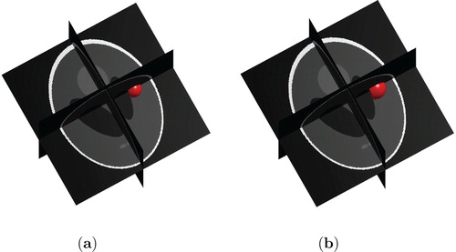
Figure 7. Low and High Grade Glioma in MRI T1 data for T=40. (a) Low Grade Glioma and (b) High Grade Glioma.

Comparing the two grown tumours obtained both after 400 iterations (corresponding to T=40), we can see that the size of the HGG tumour is larger than the LGG tumour in both the 3d Shepp–Logan set-up and in the MRI T1 model.

To further illustrate the growth in time, Figures 8–11 show, respectively, the progression in time ((a) T=20, (b) T=60 and (c) T=80) of LGG and HGG tumours for the two types of data set-ups.

Figure 8. Growth of LGG in the 3d Shepp–Logan image. (a) T=20. (b) T=60. (c) T=80.

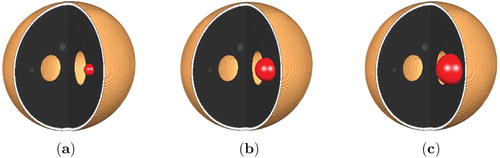
Figure 9. Growth of LGG in the MRI T1 data.(a) T=20. (b) T=60. (c) T=80.

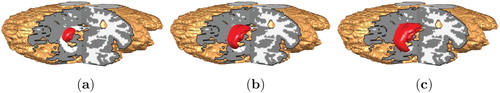
Figure 10. Growth of HGG in the 3d Shepp–Logan image. (a) T=20, (b) T=60 and (c) T=80.

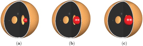
Figure 11. Growth of HGG in the MRI T1 data. (a) T=20, (b) T=60 and (c) T=80.

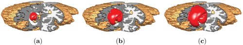
We observe that the tumour grows almost smoothly and uniformly in the simple geometric structure (shown in Figure 2) of the 3d Shepp–Logan image, see Figures 8 and 10. On the other hand, within the more complex geometric structure (shown in Figure 3) of the MRI T1 image, the tumour grows to become irregular in shape, see Figures 9 and 11.

Figures 12 and 13 show the shape that an advanced stage HGG tumour have grown to at time T=100 in respectively the 3d Shepp–Logan set-up and the MRI T1 data. From these figures, we see that the model automatically takes into account the boundaries of the tumour progression. The ring-shaped formation on the tumour in Figure 12 is due to the fact that the tumour has grown to reach the boundary of the brain and is is pushing towards the skull. The irregularities on the surface of the tumour in Figure 13 is explained likewise.

Figure 12. Grown advanced HGG shown in the 3d Shepp–Logan image.

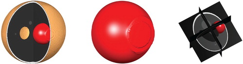
Figure 13. Grown advanced HGG shown in the T1 MRI data.

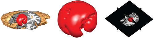
Moreover, we note that the tumour does not grow outside the skull as shown in the 3d Shepp–Logan image (Figure 12) nor in the ventricles as shown the MRI T1 data (Figure 13).

We have also generated the similar Figures 12 and 13 for the exponential and Gompertz models (see (1(1) $f\left(u\right)=\left\{\begin{array}{ll}\rho u& \alpha =1,\beta =1,\gamma =0\mathrm{Exponential},\\ \rho u(1-u)& \alpha =1,\beta =1,\gamma =1\mathrm{Logistic},\\ -\rho u\ln \left(u\right)& \alpha =1,\beta \to +\mathrm{\infty },\gamma =1\mathrm{Gompertz},\end{array}\right.$(1) ) for parameters). Rather than overloading the presentation with figures, we report the following leaving out the figures. We observed similar growth patterns for the exponential and the Gompertz models in both the Shepp–Logan model and the T1 MR1 image.

We end this section with some information about the computations. The numerical simulations presented are done in MATLAB R2016a version 9.0 and executed on an ordinary workstation having an Intel(R) Core(TM) i5-5200U CPU at 2.20 GHz. The total number of voxels in the Shepp–Logan model is $256\times 256\times 256$ and for the MRI T1-weighted brain scan it is $256\times 256\times 54$ (we have not taking into account any differences of resolutions in the x -, y- and z -directions). The total simulation time to generate Figures 12 and 13 are about 3 hours 30 minutes, respectively, 29 minutes. No optimization of the code has been done and it is believed that computational time can be further improved.

7. Conclusion

Reaction–diffusion equations have been surveyed and used in studying the growth of brain tumours. Clinical and mathematical properties of the model have been discussed, as well as a variational formulation. Full three-dimensional numerical simulations have been performed for two different set-ups, the 3d Shepp–Logan phantom and T1 MRI data from IBSR, and for both low and high grade glioma. Standard finite difference discretization of the space and time-derivatives are employed, generating a simplistic approach that performs well. Already this basic model has the realistic properties seen in the simulations such as automatic control that the tumour does not grow outside the skull. In fact, simulations show how the tumour deforms when it reaches regions into which it cannot grow further.

Disclosure statement

No potential conflict of interest was reported by the authors.

Additional information

Funding

The first author is grateful for support by the EU funding under the program ALYSSA (ERASMUS MUNDUS Action 2, Lot 6).

References

- F. Åström, Variational tensor-based models for image diffusion in non-linear domains, Ph.D. diss., Linköping University Electronic Press, 2015.
- D. Basanta, M. Simon, H. Hatzikirou, and A. Deutsch, Evolutionary game theory elucidates the role of glycolysis in glioma progression and invasion, Cell. Prolif. 41 (2008), pp. 980–987. doi: 10.1111/j.1365-2184.2008.00563.x
- G. Bastay, V.A. Kozlov, and B.O. Turesson, Iterative methods for an inverse heat conduction problem, J. Inverse Ill-posed Probl. 9 (2001), pp. 375–388. doi: 10.1515/jiip.2001.9.4.375
- S. Benzekry, C. Lamont, A. Beheshti, A. Tracz, J.M. Ebos, L. Hlatky, and P. Hahnfeldt, Classical mathematical models for description and prediction of experimental tumor growth, PLoS. Comput. Biol. 10 (2014), pp. e1003800. doi: 10.1371/journal.pcbi.1003800
- P.K. Burgess, P.M. Kulesa, J.D. Murray, and E.C. Alvord, The interaction of growth rates and diffusion coefficients in a three-dimensional mathematical model of gliomas, J. Neuropath. Exp. Neur. 56 (1997), pp. 704–713. doi: 10.1097/00005072-199706000-00008
- P.G. Ciarlet, The Finite Element Method for Elliptic Problems, North Holland, Amsterdam, 1978.
- O. Clatz, M. Sermesant, P.Y. Bondiau, H. Delingette, S.K. Warfield, G. Malandain, and N. Ayache, Realistic simulation of the 3-D growth of brain tumors in MR images coupling diffusion with biomechanical deformation, Med. Imag. IEEE T. 24 (2005), pp. 1334–1346. doi: 10.1109/TMI.2005.857217
- C. Cocosco, V. Kollokian, R. Kwan, and A. Evans, Brainweb: Online interface to a 3d simulated brain database, Neuroimage 5 (1997), p. S425.
- D.L. Collins, A.P. Zijdenbos, V. Kollokian, J.G. Sled, N.J. Kabani, C.J. Holmes, and A.C. Evans, Design and construction of a realistic digital brain phantom, IEEE Trans. Med. Imag. 17 (1998), pp. 463–468. doi: 10.1109/42.712135
- G.C. Cruywagen, D.E. Woodward, P. Tracqui, G.T. Bartoo, J. Murray, and E.C. Alvord, The modelling of diffusive tumours, J. Biol. Syst. 3 (1995), pp. 937–945. doi: 10.1142/S0218339095000836
- L.M. DeAngelis, Brain tumors, New Engl. J. Med. 344 (2001), pp. 114–123. doi: 10.1056/NEJM200101113440207
- A. Drevelegas and N. Papanikolaou, Imaging Modalities in Brain Tumors, Springer, Berlin, Heidelberg, 2011.
- L. Fass, Imaging and cancer: A review, Mol. Oncol. 2 (2008), pp. 115–152. doi: 10.1016/j.molonc.2008.04.001
- J. Ferlay, I. Soerjomataram, R. Dikshit, S. Eser, C. Mathers, M. Rebelo, D.M. Parkin, D. Forman, and F. Bray, Cancer incidence and mortality worldwide: Sources, methods and major patterns in globocan 2012, Int. J. Cancer 136 (2015), pp. E359–E386. doi: 10.1002/ijc.29210
- A. Gholami, A. Mang, and G. Biros, An inverse problem formulation for parameter estimation of a reaction–diffusion model of low grade gliomas, J. Math. Biol. 72 (2016), pp. 409–433. doi: 10.1007/s00285-015-0888-x
- A. Giese, L. Kluwe, B. Laube, H. Meissner, M.E. Berens, and M. Westphal, Migration of human glioma cells on myelin, Neurosurgery 38 (1996), pp. 755–764. doi: 10.1227/00006123-199604000-00026
- M.L. Goodenberger and R.B. Jenkins, Genetics of adult glioma, Cancer Genet. 205 (2012), pp. 613–621. doi: 10.1016/j.cancergen.2012.10.009
- D. Hanahan and R.A. Weinberg, Hallmarks of cancer: The next generation, Cell 144 (2011), pp. 646–674. doi: 10.1016/j.cell.2011.02.013
- C. Hogea, C. Davatzikos, and G. Biros, An image-driven parameter estimation problem for a reaction–diffusion glioma growth model with mass effects, J. Math. Biol. 56 (2008), pp. 793–825. doi: 10.1007/s00285-007-0139-x
- Ibsr, Internet Brain Segmentation Repository. Available at www.nitrc.org/projects/ibsr/ (accessed March 2016).
- R. Jaroudi, Inverse mathematical models for brain tumour growth, Licentiate thesis, Linköping University Electronic Press, 2017.
- R. Jaroudi, G. Baravdish, F. Åström, and B.T. Johansson, Source localization of reaction–diffusion models for brain tumors, German Conference on Pattern Recognition, Springer, 2016, pp. 414–425.
- R. Jaroudi, G. Baravdish, B.T. Johansson, and F. Åström, Numerical reconstruction of brain tumours, Inverse Probl. Sci. Eng. 27 (2019), pp. 278–298. doi: 10.1080/17415977.2018.1456537
- S. Jbabdi, E. Mandonnet, H. Duffau, L. Capelle, K.R. Swanson, M. Pélégrini-Issac, R. Guillevin, and H. Benali, Simulation of anisotropic growth of low-grade gliomas using diffusion tensor imaging, Magn. Reson. Med. 54 (2005), pp. 616–624. doi: 10.1002/mrm.20625
- J. Kačur, Method of Rothe in Evolution Equations, B. G. Teubner, Leipzig, 1985.
- A. Kansal, S. Torquato, G. Harsh, E. Chiocca, and T. Deisboeck, Simulated brain tumor growth dynamics using a three-dimensional cellular automaton, J. Theoret. Biol. 203 (2000), pp. 367–382. doi: 10.1006/jtbi.2000.2000
- P. Kleihues, P.C. Burger, and B.W. Scheithauer, The new who classification of brain tumours, Brain Pathol. 3 (1993), pp. 255–268. doi: 10.1111/j.1750-3639.1993.tb00752.x
- E. Konukoglu, O. Clatz, B.H. Menze, B. Stieltjes, M.A. Weber, E. Mandonnet, H. Delingette, and N. Ayache, Image guided personalization of reaction–diffusion type tumor growth models using modified anisotropic eikonal equations, IEEE. Trans. Med. Imaging 29 (2010), pp. 77–95. doi: 10.1109/TMI.2009.2026413
- O.A. Ladyženskaja, V.A. Solonnikov, and N.N. Ural'ceva, Linear and quasilinear equations of parabolic type, Translated from the Russian by S. Smith, Translations of Mathematical Monographs, Vol. 23, American Mathematical Society, Providence, R.I., 1968.
- J.L. Lions and E. Magenes, Non-homogeneous Boundary Value Problems and Applications, Vol. I, Springer-Verlag, New York-Heidelberg, 1972, Translated from the French by P. Kenneth, Die Grundlehren der mathematischen Wissenschaften, Band 182.
- J.L. Lions and E. Magenes, Non-homogeneous Boundary Value Problems and Applications, Vol. II, Springer-Verlag, New York-Heidelberg, 1972, Translated from the French by P. Kenneth, Die Grundlehren der mathematischen Wissenschaften, Band 182.
- D.N. Louis, A. Perry, G. Reifenberger, A. von Deimling, D. Figarella-Branger, W.K. Cavenee, H. Ohgaki, O.D. Wiestler, P. Kleihues, and D.W. Ellison, The 2016 world health organization classification of tumors of the central nervous system: A summary, Acta. Neuropathol. 131 (2016), pp. 803–820. doi: 10.1007/s00401-016-1545-1
- M.C. Mabray, R.F. Barajas, and S. Cha, Modern brain tumor imaging, Brain Tumor Res. Treat. 3 (2015), pp. 8–23. doi: 10.14791/btrt.2015.3.1.8
- M. Marušić, Ž. Bajzer, J. Freyer, and S. Vuk-Pavlović, Analysis of growth of multicellular tumour spheroids by mathematical models, Cell. Prolif. 27 (1994), pp. 73–94. doi: 10.1111/j.1365-2184.1994.tb01407.x
- J.D. Murray, Mathematical Biology. I An Introduction Interdisciplinary Applied Mathematics V. 17, Springer-Verlag, New York, 2001.
- J.D. Murray, Mathematical Biology. II Spatial Models and Biomedical Applications Interdisciplinary Applied Mathematics V. 18, Springer-Verlag, New York, 2002.
- J. Nocedal and S. Wright, Numerical Optimization, Springer Series in Operations Research and Financial Engineering, Springer New York, 2006.
- A. Pazy, Semigroups of Linear Operators and Applications to Partial Differential Equations, Springer-Verlag, New York, 1983.
- I. Rekik, S. Allassonnière, O. Clatz, E. Geremia, E. Stretton, H. Delingette, and N. Ayache, Tumor growth parameters estimation and source localization from a unique time point: Application to low-grade gliomas, Comput. Vis. Image Underst. 117 (2013), pp. 238–249. doi: 10.1016/j.cviu.2012.11.001
- Release name, Male subject, t1-weighted brain scan: 788_6. Available at www.nitrc.org/frs/shownotes.php?release_id=2305 (accessed March 2016).
- T. Roubíček, Nonlinear Partial Differential Equations with Applications, International Series of Numerical Mathematics, Vol. 153, Birkhäuser Verlag, Basel, 2005.
- L.A. Shepp and B.F. Logan, The Fourier reconstruction of a head section, IEEE. Trans. Nucl. Sci. 21 (1974), pp. 21–43. doi: 10.1109/TNS.1974.6499235
- K.R. Swanson, E. Alvord, and J. Murray, A quantitative model for differential motility of gliomas in grey and white matter, Cell. Prolif. 33 (2000), pp. 317–329. doi: 10.1046/j.1365-2184.2000.00177.x
- K.R. Swanson, E. Alvord, and J. Murray, Virtual brain tumours (gliomas) enhance the reality of medical imaging and highlight inadequacies of current therapy, Br. J. Cancer 86 (2002), pp. 14–18. doi: 10.1038/sj.bjc.6600021
- P. Tracqui, From passive diffusion to active cellular migration in mathematical models of tumour invasion, Acta. Biotheor. 43 (1995), pp. 443–464. doi: 10.1007/BF00713564
- D. Woodward, J. Cook, P. Tracqui, G. Cruywagen, J. Murray, and E. Alvord, A mathematical model of glioma growth: The effect of extent of surgical resection, Cell Prolif. 29 (1996), pp. 269–288. doi: 10.1111/j.1365-2184.1996.tb01580.x