Discontinuous Galerkin for the wave equation: a simplified a priori error analysis

Abstract

Standard discontinuous Galerkin methods, based on piecewise polynomials of degree $\mathrm{q}=0,1$, are considered for temporal semi-discretization for second-order hyperbolic equations. The main goal of this paper is to present a simple and straightforward a priori error analysis of optimal order with minimal regularity requirement on the solution. Uniform norm in time error estimates are also proved. To this end, energy identities and stability estimates of the discrete problem are proved for a slightly more general problem. These are used to prove optimal order a priori error estimates with minimal regularity requirement on the solution. The combination with the classic continuous Galerkin finite element discretization in space variable is used to formulate a full-discrete scheme. The a priori error analysis is presented. Numerical experiments are performed to verify the theoretical results.

Keywords:

• Second-order hyperbolic problems
• wave equation
• discontinuous Galerkin method
• stability estimate
• a priori error estimate

2010 AMS SUBJECT CLASSIFICATIONS:

• 65M60
• 35L05

1. Introduction

We study a priori error analysis of the discontinuous Galerkin methods of order $\mathrm{q}=0,1$, dG($\mathrm{q}$), for temporal semi-discretization of the second-order hyperbolic problems (1) $\ddot{u}+Au=f,t\in (0,T),\mathrm{w}\mathrm{i}\mathrm{t}\mathrm{h}u\left(0\right)=u_0,\dot{u}\left(0\right)=v_0,$(1) where A is a self-adjoint, positive definite, uniformly elliptic second-order operator on a Hilbert space H. We then combine the dG($\mathrm{q}$) method with a standard continuous Galerkin of order $\mathrm{r}\ge 1$, cG($\mathrm{r}$), for spatial discretization to formulate a full discrete scheme, to be called dG($\mathrm{q}$)-cG($\mathrm{r}$).

We may consider, as a prototype equation for such second-order hyperbolic equations, $A=-\mathrm{\Delta }$ with homogeneous Dirichlet boundary conditions. That is, the classical wave equation, (2) $\begin{array}{ll}\ddot{u}(x,t)-\mathrm{\Delta }u(x,t)=f(x,t)& \mathrm{i}\mathrm{n}\mathrm{\Omega }\times (0,T),\\ u(x,t)=0& \mathrm{o}\mathrm{n}\mathrm{\Gamma }\times (0,T),\\ u(x,0)=u_0\left(x\right),\dot{u}(x,0)=v_0\left(x\right)& \mathrm{i}\mathrm{n}\mathrm{\Omega },\end{array}$(2) where Ω is a bounded and convex polygonal domain in ${\mathbb{R}}^d$, $d\in \{1,2,3\}$, with boundary Γ. We denote $\dot{u}=\frac{\mathrm{\partial }u}{\mathrm{\partial }t}$ and $\ddot{u}=\frac{{\mathrm{\partial }}^{2}u}{\mathrm{\partial }{t}^2}$. The present work also applies to wave phenomena with vector-valued solution $u:\mathrm{\Omega }\times (0,T)\to {\mathbb{R}}^d$, such as wave elasticity.

We may also consider more general equations (3) $\ddot{u}+\tilde{A}u=f,t\in (0,T),\mathrm{w}\mathrm{i}\mathrm{t}\mathrm{h}u\left(0\right)=u_0,\dot{u}\left(0\right)=v_0,$(3) where $\tilde{A}=-\mathrm{\nabla }\cdot \kappa \mathrm{\nabla }$. That is, (4) $\begin{array}{ll}\ddot{u}(x,t)-\mathrm{\nabla }\cdot \kappa \mathrm{\nabla }u(x,t)=f(x,t)& \mathrm{i}\mathrm{n}\mathrm{\Omega }\times (0,T),\\ u(x,t)=0& \mathrm{o}\mathrm{n}\mathrm{\Gamma }\times (0,T),\\ u(x,0)=u_0\left(x\right),\dot{u}(x,0)=v_0\left(x\right)& \mathrm{i}\mathrm{n}\mathrm{\Omega }.\end{array}$(4) Here $\kappa \left(x\right)$ is a smooth function and for two positive constants ${\kappa }_{min}$ and ${\kappa }_{max}$, ${\kappa }_{min}\le \kappa \left(x\right)\le {\kappa }_{max},x\in \mathrm{\Omega }.$We note that $\kappa \left(x\right)$ can also be a uniformly symmetric positive definite matrix.

Throughout this paper, for simplicity, we consider (2(2) $\begin{array}{ll}\ddot{u}(x,t)-\mathrm{\Delta }u(x,t)=f(x,t)& \mathrm{i}\mathrm{n}\mathrm{\Omega }\times (0,T),\\ u(x,t)=0& \mathrm{o}\mathrm{n}\mathrm{\Gamma }\times (0,T),\\ u(x,0)=u_0\left(x\right),\dot{u}(x,0)=v_0\left(x\right)& \mathrm{i}\mathrm{n}\mathrm{\Omega },\end{array}$(2) ), and we remark on how the approach is applied to (4(4) $\begin{array}{ll}\ddot{u}(x,t)-\mathrm{\nabla }\cdot \kappa \mathrm{\nabla }u(x,t)=f(x,t)& \mathrm{i}\mathrm{n}\mathrm{\Omega }\times (0,T),\\ u(x,t)=0& \mathrm{o}\mathrm{n}\mathrm{\Gamma }\times (0,T),\\ u(x,0)=u_0\left(x\right),\dot{u}(x,0)=v_0\left(x\right)& \mathrm{i}\mathrm{n}\mathrm{\Omega }.\end{array}$(4) ), too. The results and the corresponding proofs for $\tilde{A}$ are very similar to case A, and, therefore, we will omit the proofs.

The discontinuous Galerkin-type methods for time or space discretization have been studied extensively in the literature for ordinary differential equations and parabolic/hyperbolic partial differential equations; see, for example, Refs. [1,3–6,8,10,13,16,18,19,21,24,27,28] and the references therein. In particular, several discontinuous and continuous Galerkin finite element methods, both in time and space variables, for solving second-order hyperbolic equations have appeared in the literature, see, e.g. Refs. [1,11,12,14,25] and the references therein.

A dG(1)-cG(1) methods was studied in Ref. [14]. This was extended by the study in Ref. [1], where dG time-stepping methods were applied directly to the second-order ode system that arise from spatial semi-discretization by standard cG methods. Discontinuous spatial discretization of wave problems were studied in Refs. [12,20,25].

Uniform in time stability analysis, also so-called strong stability or $L_{\mathrm{\infty }}$-stability, has been studied for parabolic problems, [9,18,27], but not for second-order hyperbolic problems. An important tool for such analysis of parabolic problems is the smoothing property of the solution operator, thanks to analytic semigroup. For parabolic problems, in Ref. [9], uniform in time stability and error estimates for dG($\mathrm{q}$), $\mathrm{q}\ge 0$, have been proved using the Dunford-Taylor formula based on smoothing properties of the analytic semigroups. For parabolic problems which are perturbed by a memory term, such analysis has been done for dG(0) and dG(1), using the linearity of the basis functions in time [18]. Another way to analyse uniform in time stability is using a lifting operator technique to write the dG($\mathrm{q}$) formulation in a strong (pointwise) form [27].

Second-order hyperbolic problems, unfortunately, do not enjoy such smoothing properties, due to the fact that the solution operator generates a $C_0$-semigroup only, but not an analytic semigroup. However, one can use the linearity of the basis function in time in case of dG(0) and dG(1) to prove such a priori error estimates, which is a part of this work.

Optimal order $L_{\mathrm{\infty }}\left(\right[0,\mathrm{\infty }),L_2(\mathrm{\Omega }\left)\right)$ estimates for Galerkin finite element approximation of the wave equation were first obtained by the study in Ref. [7], and the regularity requirement for the initial displacement was not minimal. This was improved in Ref. [2], and in Ref. [23], it was shown that the resulting regularity requirement is optimal; see [15, Lemma 4.4] for more details. A new approach was introduced for a priori error analysis of the second-order hyperbolic problems in the context of continuous Galerkin methods, spatial semi-discretization cG(1) in Ref. [15] and cG(1)-cG(1) in Ref. [17].

Here, we extend such a priori error analysis to dG($\mathrm{q}$) time-stepping for $\mathrm{q}=0,1$, for (2(2) $\begin{array}{ll}\ddot{u}(x,t)-\mathrm{\Delta }u(x,t)=f(x,t)& \mathrm{i}\mathrm{n}\mathrm{\Omega }\times (0,T),\\ u(x,t)=0& \mathrm{o}\mathrm{n}\mathrm{\Gamma }\times (0,T),\\ u(x,0)=u_0\left(x\right),\dot{u}(x,0)=v_0\left(x\right)& \mathrm{i}\mathrm{n}\mathrm{\Omega },\end{array}$(2) ), as the chief example for (1(1) $\ddot{u}+Au=f,t\in (0,T),\mathrm{w}\mathrm{i}\mathrm{t}\mathrm{h}u\left(0\right)=u_0,\dot{u}\left(0\right)=v_0,$(1) ). We also present the a priori error analysis for a full discrete scheme by combining dG($\mathrm{q}$) with a standard cG($\mathrm{r}$), $\mathrm{r}\ge 1$, method for spatial discretization (see also Remark 3.1). The regularity requirements on the solution are minimal, which is important, in particular, for stochastic model problems and for second-order hyperbolic partial differential equations perturbed by a memory term, see Refs. [15,17,26]. The approach presented here is simple and straightforward such that we can prove error estimates in several space-time norms. We also show how the same approach is used to prove uniform in time error estimates. We note that the error analysis in Ref. [17] is based on energy arguments, while in Ref. [26], it is via duality arguments. That is, we can use the presented approach of error analysis of dG methods via duality arguments, too.

To prove a priori error estimates at the time-mesh points and also uniform in time, we prove stability estimates and energy identity, respectively, for the discrete problem of a more general form, by considering an extra (artificial) load term in the so-called displacement-velocity formulation (see Remark 4.1). This gives the flexibility to obtain optimal order a priori error estimates with minimal regularity requirement on the solution. See Remark 4.2, too. For dG methods, long-time integration without error accumulation is possible since the stability constants are independent of the length of the time interval; see also Remark 6.1.

The outline of this paper is as follows. We provide some preliminaries and the weak formulation of the model problem, in § 2. In Section 3, we formulate the dG($\mathrm{q}$) method, and we obtain energy identity and stability estimates for the discrete problem of a slightly more general form. Then, in § 4, we prove optimal order a priori error estimates in $L_2$ and $H^1$ norms for the displacement and $L_2$-norm of the velocity, with minimal regularity requirement on the solution. We also prove uniform in time a priori error estimates. In § 5, we formulate the dG($\mathrm{q}$)-cG($\mathrm{r}$) scheme and study the stability of the discrete problem, to be used to prove a priori error estimates in Section 6. Finally, numerical experiments are presented in Section 7 in order to illustrate the theory.

2. Preliminaries

We let $H=L_2\left(\mathrm{\Omega }\right)$ with the inner product $(\cdot ,\cdot )$ and the induced norm $\Vert \cdot \Vert$. Denote $\mathcal{V}=H_0^1\left(\mathrm{\Omega }\right)=\{u\in H^1(\mathrm{\Omega }):u{|}_{\mathrm{\Gamma }}=0\}$ with the energy inner product $a(\cdot ,\cdot )=(\mathrm{\nabla }\cdot ,\mathrm{\nabla }\cdot )$ and the induced norm $\Vert \cdot {\Vert }_{\mathcal{V}}$. Let $A=-\mathrm{\Delta }$ be defined with homogeneous Dirichlet boundary conditions on $\mathrm{d}\mathrm{o}\mathrm{m}\left(A\right)=H^2\left(\mathrm{\Omega }\right)\cap \mathcal{V}$, and $\left\{\right({\lambda }_k,{\phi }_k){\}}_{k=1}^{\mathrm{\infty }}$ be the eigenpairs of A, i.e. $A{\phi }_k={\lambda }_k{\phi }_k,k\in \mathbb{N}.$It is known that $0<{\lambda }_1\le {\lambda }_2\le \cdots \le {\lambda }_k\le \cdots$ with $\underset{k\to \mathrm{\infty }}{lim}{\lambda }_k=\mathrm{\infty }$ and the eigenvectors $\{{\phi }_k{\}}_{k=1}^{\mathrm{\infty }}$ form an orthonormal basis for H. Then $(A^{l}u,v)=\sum _{k=1}^{\mathrm{\infty }}{\lambda }_k^l(u,{\phi }_k)(v,{\phi }_k),$and we introduce the fractional-order spaces [28], ${\dot{H}}^{\alpha }=\mathrm{d}\mathrm{o}\mathrm{m}\left(A^{\frac{\alpha }{2}}\right),\Vert v{\Vert }_{\alpha }^2:=\Vert A^{\frac{\alpha }{2}}v{\Vert }^2=\sum _{k=1}^{\mathrm{\infty }}{\lambda }_k^{\alpha }(v,{\phi }_k{)}^2,\alpha \in \mathbb{R},v\in \dot{\phantom{a}}{H}^{\alpha }.$We note that $H={\dot{H}}^0$ and $\mathcal{V}={\dot{H}}^1$. Defining the new variables $u_1=u$ and $u_2=\dot{u}$, we can write the velocity-displacement form of (2(2) $\begin{array}{ll}\ddot{u}(x,t)-\mathrm{\Delta }u(x,t)=f(x,t)& \mathrm{i}\mathrm{n}\mathrm{\Omega }\times (0,T),\\ u(x,t)=0& \mathrm{o}\mathrm{n}\mathrm{\Gamma }\times (0,T),\\ u(x,0)=u_0\left(x\right),\dot{u}(x,0)=v_0\left(x\right)& \mathrm{i}\mathrm{n}\mathrm{\Omega },\end{array}$(2) ) as $\begin{array}{ll}-\mathrm{\Delta }{\dot{u}}_1+\mathrm{\Delta }{u}_2=0& \mathrm{i}\mathrm{n}\mathrm{\Omega }\times (0,T),\\ {\dot{u}}_2-\mathrm{\Delta }{u}_1=f& \mathrm{i}\mathrm{n}\mathrm{\Omega }\times (0,T),\\ u_1=u_2=0& \mathrm{o}\mathrm{n}\mathrm{\Gamma }\times (0,T),\\ u_1(\cdot ,0)=u_0,u_2(\cdot ,0)=v_0& \mathrm{i}\mathrm{n}\mathrm{\Omega },\end{array}$for which the weak form is to find $u_1\left(t\right)$ and $u_2\left(t\right)\in \mathcal{V}$ such that (5) $\begin{array}{l}a\left({\dot{u}}_1\right(t),v_1)-a\left(u_2\right(t),v_1)=0,\\ \left({\dot{u}}_2\right(t),v_2)+a\left(u_1\right(t),v_2)=\left(f\right(t),v_2),\mathrm{\forall }{v}_1,v_2\in \mathcal{V},t\in (0,T),\\ u_1\left(0\right)=u_0,u_2\left(0\right)=v_0.\end{array}$(5) This equation is used for dG($\mathrm{q}$) formulation.

Remark 2.1

For $\tilde{A}=-\mathrm{\nabla }\cdot \kappa \mathrm{\nabla }$ in (4(4) $\begin{array}{ll}\ddot{u}(x,t)-\mathrm{\nabla }\cdot \kappa \mathrm{\nabla }u(x,t)=f(x,t)& \mathrm{i}\mathrm{n}\mathrm{\Omega }\times (0,T),\\ u(x,t)=0& \mathrm{o}\mathrm{n}\mathrm{\Gamma }\times (0,T),\\ u(x,0)=u_0\left(x\right),\dot{u}(x,0)=v_0\left(x\right)& \mathrm{i}\mathrm{n}\mathrm{\Omega }.\end{array}$(4) ), with homogeneous Dirichlet boundary conditions on $\mathrm{d}\mathrm{o}\mathrm{m}\left(\tilde{A}\right)=H^2\left(\mathrm{\Omega }\right)\cap \mathcal{V}$, we denote by $\left\{\right({\tilde{\lambda }}_k,{\tilde{\phi }}_k){\}}_{k=1}^{\mathrm{\infty }}$ the eigenpairs of $\tilde{A}$, i.e. $\tilde{A}{\tilde{\phi }}_k={\tilde{\lambda }}_k{\tilde{\phi }}_k,k\in \mathbb{N}.$Then $0<{\tilde{\lambda }}_1\le {\tilde{\lambda }}_2\le \cdots \le {\tilde{\lambda }}_k\le \cdots$ with $\underset{k\to \mathrm{\infty }}{lim}{\tilde{\lambda }}_k=\mathrm{\infty }$ and the eigenvectors $\{{\tilde{\phi }}_k{\}}_{k=1}^{\mathrm{\infty }}$ form an orthonormal basis for H. Having $({\tilde{A}}^{l}u,v)=\sum _{k=1}^{\mathrm{\infty }}{\tilde{\lambda }}_k^l(u,{\tilde{\phi }}_k)(v,{\tilde{\phi }}_k),$we can introduce the fractional-order spaces ${\dot{\tilde{H}}}^{\alpha }=\mathrm{d}\mathrm{o}\mathrm{m}\left({\tilde{A}}^{\frac{\alpha }{2}}\right),|||v||{|}_{\alpha }^2:=\Vert {\tilde{A}}^{\frac{\alpha }{2}}v{\Vert }^2=\sum _{k=1}^{\mathrm{\infty }}{\tilde{\lambda }}_k^{\alpha }(v,{\tilde{\phi }}_k{)}^2,\alpha \in \mathbb{R},v\in {\dot{\tilde{H}}}^{\alpha }.$We note that $H={\dot{\tilde{H}}}^0$ and $\mathcal{V}={\dot{\tilde{H}}}^1$. If we define an energy inner product $\tilde{a}(\cdot ,\cdot )=(\kappa \mathrm{\nabla }\cdot ,\mathrm{\nabla }\cdot )$ with the induced norm $|||\cdot ||{|}_{\mathcal{V}}$, then the norms $|||\cdot ||{|}_{\mathcal{V}}$ and $\Vert \cdot {\Vert }_{\mathcal{V}}$ are equivalent on $\mathcal{V}$, that is ${\kappa }_{min}\Vert v{\Vert }_{\mathcal{V}}\le |||v||{|}_{\mathcal{V}}\le {\kappa }_{max}\Vert v{\Vert }_{\mathcal{V}},v\in \mathcal{V}.$We also note that the norms $\Vert \cdot {\Vert }_{\alpha }$ and $|||\cdot ||{|}_{\alpha }$ are equivalent on ${\dot{H}}^{\alpha }$.

Then, the weak form of (4(4) $\begin{array}{ll}\ddot{u}(x,t)-\mathrm{\nabla }\cdot \kappa \mathrm{\nabla }u(x,t)=f(x,t)& \mathrm{i}\mathrm{n}\mathrm{\Omega }\times (0,T),\\ u(x,t)=0& \mathrm{o}\mathrm{n}\mathrm{\Gamma }\times (0,T),\\ u(x,0)=u_0\left(x\right),\dot{u}(x,0)=v_0\left(x\right)& \mathrm{i}\mathrm{n}\mathrm{\Omega }.\end{array}$(4) ) is to find $u_1\left(t\right)$ and $u_2\left(t\right)\in \mathcal{V}$ such that (6) $\begin{array}{rl}& \tilde{a}\left({\dot{u}}_1\right(t),v_1)-\tilde{a}\left(u_2\right(t),v_1)=0,\\ & \left({\dot{u}}_2\right(t),v_2)+\tilde{a}\left(u_1\right(t),v_2)=\left(f\right(t),v_2),\mathrm{\forall }{v}_1,v_2\in \mathcal{V},t\in (0,T),\\ & u_1\left(0\right)=u_0,u_2\left(0\right)=v_0.\end{array}$(6) This equation then can be used for the dG($\mathrm{q}$) formulation.

3. The discontinuous Galerkin time discretization

In this section, we apply the standard dG method in time variable using piecewise polynomials of degree $\mathrm{q}=0,1$, and we investigate the stability.

3.1. dG($\mathrm{q}$) formulation

Let $0=t_0<t_1<\cdots <t_N=T$ be a temporal mesh with time subintervals $I_n=(t_{n-1},t_n)$ and steps $k_n=t_n-t_{n-1}$, and the maximum step-size by $k=\underset{1\le n\le N}{max}{k}_n$. Let ${\mathbb{P}}_{\mathrm{q}}={\mathbb{P}}_{\mathrm{q}}\left(\mathcal{V}\right)=\{v:v(t)=\sum _{j=0}^{\mathrm{q}}{v}_j{t}^j,v_j\in \mathcal{V}\}$ and define the finite element space ${\mathcal{V}}_{\mathrm{q}}=\{v:v{|}_{S_n}\in {\mathbb{P}}_{\mathrm{q}}(\mathcal{V}),n=1,\dots ,N\}$ for each space-time 'Slab' $S^n=\mathrm{\Omega }\times I_n$.

We follow the usual convention that a function $U=(U_1,U_2)\in {\mathcal{V}}_{\mathrm{q}}\times {\mathcal{V}}_{\mathrm{q}}$ is left-continuous at each time level $t_n$ and we define $U_{i,n}^{\pm }=\underset{s\to 0^{\pm }}{lim}{U}_i(t_n+s)$, writing $U_{i,n}^{-}=U_i\left(t_n^{-}\right),U_{i,n}^{+}=U_i\left(t_n^{+}\right),{\left[U_i\right]}_n=U_{i,n}^{+}-U_{i,n}^{-}\mathrm{f}\mathrm{o}\mathrm{r}i=1,2.$The dG method determines $U=(U_1,U_2)\in {\mathcal{V}}_{\mathrm{q}}\times {\mathcal{V}}_{\mathrm{q}}$ on $S^n\times S^n$ for $n=1,\dots ,N$ by setting $U_0^{-}=(U_{1,0}^{-},U_{2,0}^{-})$, and then (7) $\begin{array}{rl}& {\int }_{I_n}(a({\dot{U}}_1,V_1)-a(U_2,V_1))\mathrm{d}t+a(U_{1,n-1}^{+},V_{1,n-1}^{+})=a(U_{1,n-1}^{-},V_{1,n-1}^{+}),\\ & {\int }_{I_n}(({\dot{U}}_2,V_2)+a(U_1,V_2))\mathrm{d}t+(U_{2,n-1}^{+},V_{2,n-1}^{+})\\ & =(U_{2,n-1}^{-},V_{2,n-1}^{+})+{\int }_{I_n}(f,V_2)\mathrm{d}t,\mathrm{\forall }V=(V_1,V_2)\in {\mathbb{P}}_{\mathrm{q}}\times {\mathbb{P}}_{\mathrm{q}}.\end{array}$(7) Now, we define the function space $\mathcal{W}$ consisting of functions that are piecewise smooth with respect to the temporal mesh with values in $\mathrm{d}\mathrm{o}\mathrm{m}\left(A\right)$. We note that ${\mathcal{V}}_{\mathrm{q}}\subset \mathcal{W}$. Then we define the bilinear form B and the linear form L on $\mathcal{W}\times \mathcal{W}$ by (8) $\begin{array}{rl}B\left(\right(u_1,u_2),(v_1,v_2\left)\right)& =\sum _{n=1}^N{\int }_{I_n}\{a({\dot{u}}_1,v_1)-a(u_2,v_1)+({\dot{u}}_2,v_2)+a(u_1,v_2)\}\mathrm{d}t\\ & +\sum _{n=1}^{N-1}\left\{a\right({\left[u_1\right]}_n,v_{1,n}^{+})+({\left[u_2\right]}_n,v_{2,n}^{+}\left)\right\}+a(u_{1,0}^{+},v_{1,0}^{+})+(u_{2,0}^{+},v_{2,0}^{+}),\\ L((v_1,v_2))& =\sum _{n=1}^N{\int }_{I_n}(f,v_2)\mathrm{d}t+a(u_0,v_{1,0}^{+})+(v_0,v_{2,0}^{+}).\end{array}$(8) Then $U=(U_1,U_2)\in {\mathcal{V}}_{\mathrm{q}}\times {\mathcal{V}}_{\mathrm{q}}$, the solution of discrete problem (7(7) $\begin{array}{rl}& {\int }_{I_n}(a({\dot{U}}_1,V_1)-a(U_2,V_1))\mathrm{d}t+a(U_{1,n-1}^{+},V_{1,n-1}^{+})=a(U_{1,n-1}^{-},V_{1,n-1}^{+}),\\ & {\int }_{I_n}(({\dot{U}}_2,V_2)+a(U_1,V_2))\mathrm{d}t+(U_{2,n-1}^{+},V_{2,n-1}^{+})\\ & =(U_{2,n-1}^{-},V_{2,n-1}^{+})+{\int }_{I_n}(f,V_2)\mathrm{d}t,\mathrm{\forall }V=(V_1,V_2)\in {\mathbb{P}}_{\mathrm{q}}\times {\mathbb{P}}_{\mathrm{q}}.\end{array}$(7) ), satisfies (9) $B(U,V)=L\left(V\right),\mathrm{\forall }V=(V_1,V_2)\in {\mathcal{V}}_{\mathrm{q}}\times {\mathcal{V}}_{\mathrm{q}},U_0^{-}=(U_{1,0}^{-},U_{2,0}^{-})=(u_0,v_0).$(9) We note that the solution $u=(u_1,u_2)$ of (5(5) $\begin{array}{l}a\left({\dot{u}}_1\right(t),v_1)-a\left(u_2\right(t),v_1)=0,\\ \left({\dot{u}}_2\right(t),v_2)+a\left(u_1\right(t),v_2)=\left(f\right(t),v_2),\mathrm{\forall }{v}_1,v_2\in \mathcal{V},t\in (0,T),\\ u_1\left(0\right)=u_0,u_2\left(0\right)=v_0.\end{array}$(5) ) also satisfies (10) $B(u,v)=L\left(v\right),\mathrm{\forall }v=(v_1,v_2)\in \mathcal{W}\times \mathcal{W},\left(u_1\right(0),u_2(0\left)\right)=(u_0,v_0).$(10) These imply the Galerkin orthogonality for the error $e=(e_1,e_2)=(U_1,U_2)-(u_1,u_2)$, that is, (11) $B(e,V)=0,\mathrm{\forall }V=(V_1,V_2)\in {\mathcal{V}}_{\mathrm{q}}\times {\mathcal{V}}_{\mathrm{q}}.$(11) Integration by parts yields an alternative expression for the bilinear form (8(8) $\begin{array}{rl}B\left(\right(u_1,u_2),(v_1,v_2\left)\right)& =\sum _{n=1}^N{\int }_{I_n}\{a({\dot{u}}_1,v_1)-a(u_2,v_1)+({\dot{u}}_2,v_2)+a(u_1,v_2)\}\mathrm{d}t\\ & +\sum _{n=1}^{N-1}\left\{a\right({\left[u_1\right]}_n,v_{1,n}^{+})+({\left[u_2\right]}_n,v_{2,n}^{+}\left)\right\}+a(u_{1,0}^{+},v_{1,0}^{+})+(u_{2,0}^{+},v_{2,0}^{+}),\\ L((v_1,v_2))& =\sum _{n=1}^N{\int }_{I_n}(f,v_2)\mathrm{d}t+a(u_0,v_{1,0}^{+})+(v_0,v_{2,0}^{+}).\end{array}$(8) ), as (12) $\begin{array}{rl}{B}^{\ast }(u,v)& =\sum _{n=1}^N{\int }_{I_n}\{-a(u_1,{\dot{v}}_1)-a(u_2,v_1)-(u_2,{\dot{v}}_2)+a(u_1,v_2)\}\mathrm{d}t\\ & -\sum _{n=1}^{N-1}\{a(u_{1,n}^{-},[v_1{]}_n)+(u_{2,n}^{-},\left[v_2{]}_n\right)\}+a(u_{1,N}^{-},v_{1,N}^{-})+(u_{2,N}^{-},v_{2,N}^{-}).\end{array}$(12)

Remark 3.1

We note that the framework also applies to spatial finite-dimensional function spaces ${\mathcal{V}}_{\mathrm{q},\mathrm{r}}\subset {\mathcal{V}}_{\mathrm{q}}$, such as, a continuous Galerkin finite element method of order r for discretization in space variable. One can combine a continuous Galerkin finite element method in spatial variable to get a full discrete scheme. That is the subject of Section 5.

3.2. Stability

Here, we present a stability (energy) identity and stability estimate, which are used in a priori error analysis. In our error analysis, we need a stability identity for a slightly more general problem, that is $U=(U_1,U_2)\in {\mathcal{V}}_{\mathrm{q}}\times {\mathcal{V}}_{\mathrm{q}}$ such that (13) $B(U,V)=\hat{L}\left(V\right),\mathrm{\forall }V=(V_1,V_2)\in {\mathcal{V}}_{\mathrm{q}}\times {\mathcal{V}}_{\mathrm{q}},$(13) where the linear form $\hat{L}$ is defined on $\mathcal{W}\times \mathcal{W}$ by $\hat{L}\left(\right(v_1,v_2\left)\right)=\sum _{n=1}^N{\int }_{I_n}\{a(f_1,v_1)+(f_2,v_2)\}\mathrm{d}t+a(u_0,v_{1,0}^{+})+(v_0,v_{2,0}^{+}).$That is, instead of (5(5) $\begin{array}{l}a\left({\dot{u}}_1\right(t),v_1)-a\left(u_2\right(t),v_1)=0,\\ \left({\dot{u}}_2\right(t),v_2)+a\left(u_1\right(t),v_2)=\left(f\right(t),v_2),\mathrm{\forall }{v}_1,v_2\in \mathcal{V},t\in (0,T),\\ u_1\left(0\right)=u_0,u_2\left(0\right)=v_0.\end{array}$(5) ), we study the stability of the dG($\mathrm{q}$) discretization of a more general problem $\begin{array}{l}a\left({\dot{u}}_1\right(t),v_1)-a\left(u_2\right(t),v_1)=a\left(f_1\right(t),v_1),\\ \left({\dot{u}}_2\right(t),v_2)+a\left(u_1\right(t),v_2)=\left(f_2\right(t),v_2),\mathrm{\forall }{v}_1,v_2\in \mathcal{V},t\in (0,T),\\ u_1\left(0\right)=u_0,u_2\left(0\right)=v_0.\end{array}$See Remark 4.1.

We define the following norms $\Vert u{\Vert }_{I_n}=\underset{t\in I_n}{sup}\Vert u\left(t\right)\Vert ,\mathrm{a}\mathrm{n}\mathrm{d}\Vert u{\Vert }_{s,I_n}=\underset{t\in I_n}{sup}\Vert u\left(t\right){\Vert }_s,$and $\Vert u{\Vert }_{J_N}=\underset{t\in J_N}{sup}\Vert u\left(t\right)\Vert ,\mathrm{a}\mathrm{n}\mathrm{d}\Vert u{\Vert }_{s,J_N}=\underset{t\in J_N}{sup}\Vert u\left(t\right){\Vert }_s,$where $J_N=(0,t_N)$.

Theorem 3.1

Let $U=(U_1,U_2)$ be a solution of (13(13) $B(U,V)=\hat{L}\left(V\right),\mathrm{\forall }V=(V_1,V_2)\in {\mathcal{V}}_{\mathrm{q}}\times {\mathcal{V}}_{\mathrm{q}},$(13) ). Then for any $T>0$ and $l\in \mathbb{R}$, we have the energy identity (14) $\begin{array}{rl}& \Vert U_{1,N}^{-}{\Vert }_{l+1}^2+\Vert U_{2,N}^{-}{\Vert }_l^2+\sum _{n=0}^{N-1}\{\Vert [U_1{]}_n{\Vert }_{l+1}^2+\Vert \left[U_2{]}_n{\Vert }_l^2\right\}\\ & =\Vert u_0{\Vert }_{l+1}^2+\Vert v_0{\Vert }_l^2+2{\int }_0^T\{a(f_1,A^l{U}_1)+(f_2,A^l{U}_2)\}\mathrm{d}t.\end{array}$(14) Moreover, for some constant $C>0$ (independent of T), we have the stability estimate (15) $\Vert U_{1,N}^{-}{\Vert }_{l+1}+\Vert U_{2,N}^{-}{\Vert }_l\le C(\Vert u_0{\Vert }_{l+1}+\Vert v_0{\Vert }_l+{\int }_0^T\{\Vert f_1{\Vert }_{l+1}+\Vert f_2{\Vert }_l\}\mathrm{d}t).$(15)

Proof.

We set $V_i=A^l{U}_i$ for  $i=1,2$ in (13(13) $B(U,V)=\hat{L}\left(V\right),\mathrm{\forall }V=(V_1,V_2)\in {\mathcal{V}}_{\mathrm{q}}\times {\mathcal{V}}_{\mathrm{q}},$(13) ) to obtain $\begin{array}{rl}& \frac{1}{2}\sum _{n=1}^N{\int }_{I_n}\frac{\mathrm{\partial }}{\mathrm{\partial }t}\Vert U_1{\Vert }_{l+1}^2\mathrm{d}t+\frac{1}{2}\sum _{n=1}^N{\int }_{I_n}\frac{\mathrm{\partial }}{\mathrm{\partial }t}\Vert U_2{\Vert }_l^2\mathrm{d}t\\ & +\sum _{n=1}^{N-1}\{a\left(\right[U_1{]}_n,A^l{U}_{1,n}^{+})+([U_2{]}_n,A^l{U}_{2,n}^{+})\}+a(U_{1,0}^{+},A^l{U}_{1,0}^{+})+(U_{2,0}^{+},A^l{U}_{2,0}^{+})\\ & ={\int }_0^T\{a(f_1,A^l{U}_1)+(f_2,A^l{U}_2)\}\mathrm{d}t+a(u_0,A^l{U}_{1,0}^{+})+(v_0,A^l{U}_{2,0}^{+}).\end{array}$Now writing the first two terms at the left side as $\begin{array}{rl}& \frac{1}{2}\sum _{n=1}^N{\int }_{I_n}\frac{\mathrm{\partial }}{\mathrm{\partial }t}\Vert U_1{\Vert }_{l+1}^2\mathrm{d}t+\frac{1}{2}\sum _{n=1}^N{\int }_{I_n}\frac{\mathrm{\partial }}{\mathrm{\partial }t}\Vert U_2{\Vert }_l^2\mathrm{d}t\\ & =\sum _{n=1}^{N-1}\{\frac{1}{2}\Vert U_{1,n}^{-}{\Vert }_{l+1}^2-\frac{1}{2}\Vert U_{1,n}^{+}{\Vert }_{l+1}^2\}+\frac{1}{2}\Vert U_{1,N}^{-}{\Vert }_{l+1}^2-\frac{1}{2}\Vert U_{1,0}^{+}{\Vert }_{l+1}^2\\ & +\sum _{n=1}^{N-1}\{\frac{1}{2}\Vert U_{2,n}^{-}{\Vert }_l^2-\frac{1}{2}\Vert U_{2,n}^{+}{\Vert }_l^2\}+\frac{1}{2}\Vert U_{2,N}^{-}{\Vert }_l^2-\frac{1}{2}\Vert U_{2,0}^{+}{\Vert }_l^2,\end{array}$we have $\begin{array}{rl}& \sum _{n=1}^{N-1}\{\frac{1}{2}\Vert U_{1,n}^{-}{\Vert }_{l+1}^2-\frac{1}{2}\Vert U_{1,n}^{+}{\Vert }_{l+1}^2+a([U_1{]}_n,A^l{U}_{1,n}^{+})\}+\frac{1}{2}\Vert U_{1,N}^{-}{\Vert }_{l+1}^2+\frac{1}{2}\Vert U_{1,0}^{+}{\Vert }_{l+1}^2\\ & +\sum _{n=1}^{N-1}\{\frac{1}{2}\Vert U_{2,n}^{-}{\Vert }_l^2-\frac{1}{2}\Vert U_{2,n}^{+}{\Vert }_l^2+([U_2{]}_n,A^l{U}_{2,n}^{+})\}+\frac{1}{2}\Vert U_{2,N}^{-}{\Vert }_l^2+\frac{1}{2}\Vert U_{2,0}^{+}{\Vert }_l^2\\ & =\sum _{n=1}^N{\int }_{I_n}\left\{a\right(f_1,A^l{U}_1)+(f_2,A^l{U}_2\left)\right\}\mathrm{d}t+a(U_{1,0}^{-},A^l{U}_{1,0}^{+})+(U_{2,0}^{-},A^l{U}_{2,0}^{+}).\end{array}$Then, using (for $n=1,\dots ,N-1$) $\begin{array}{rl}& \frac{1}{2}\Vert U_{1,n}^{-}{\Vert }_{l+1}^2-\frac{1}{2}\Vert U_{1,n}^{+}{\Vert }_{l+1}^2+a\left(\right[U_1{]}_n,A^l{U}_{1,n}^{+})=\frac{1}{2}\Vert [U_1{]}_n{\Vert }_{l+1}^2,\\ & \frac{1}{2}\Vert U_{2,n}^{-}{\Vert }_l^2-\frac{1}{2}\Vert U_{2,n}^{+}{\Vert }_l^2+\left(\right[U_2{]}_n,A^l{U}_{2,n}^{+})=\frac{1}{2}\Vert [U_2{]}_n{\Vert }_l^2,\end{array}$we conclude $\begin{array}{rl}& \frac{1}{2}\sum _{n=1}^{N-1}\Vert [U_1{]}_n{\Vert }_{l+1}^2+\frac{1}{2}\Vert U_{1,N}{\Vert }_{l+1}^2+\frac{1}{2}\Vert U_{1,0}^{+}{\Vert }_{l+1}^2-a(U_{1,0}^{-},A^l{U}_{1,0}^{+})\\ & +\frac{1}{2}\sum _{n=1}^{N-1}\Vert [U_2{]}_n{\Vert }_l^2+\frac{1}{2}\Vert U_{2,N}{\Vert }_l^2+\frac{1}{2}\Vert U_{2,0}^{+}{\Vert }_l^2-(U_{2,0}^{-},A^l{U}_{2,0}^{+})\\ & ={\int }_0^T\left\{a\right(f_1,A^l{U}_1)+(f_2,A^l{U}_2\left)\right\}\mathrm{d}t.\end{array}$Hence, having $\begin{array}{rl}& \frac{1}{2}\Vert U_{1,0}^{+}{\Vert }_{l+1}^2-a(A^{\frac{l}{2}}{U}_{1,0}^{-},A^{\frac{l}{2}}{U}_{1,0}^{+})=\frac{1}{2}\Vert [U_1{]}_0{\Vert }_{l+1}^2-\frac{1}{2}\Vert U_{1,0}^{-}{\Vert }_{l+1}^2,\\ & \frac{1}{2}\Vert U_{2,0}^{+}{\Vert }_l^2-(A^{\frac{l}{2}}{U}_{2,0}^{-},A^{\frac{l}{2}}{U}_{2,0}^{+})=\frac{1}{2}\Vert [U_2{]}_0{\Vert }_l^2-\frac{1}{2}\Vert U_{2,0}^{-}{\Vert }_l^2,\end{array}$we conclude the identity $\begin{array}{rl}& \frac{1}{2}\Vert U_{1,N}^{-}{\Vert }_{l+1}^2+\frac{1}{2}\Vert U_{2,N}^{-}{\Vert }_l^2+\frac{1}{2}\sum _{n=0}^{N-1}\Vert [U_1{]}_n{\Vert }_{l+1}^2+\frac{1}{2}\sum _{n=0}^{N-1}\Vert [U_2{]}_n{\Vert }_l^2\\ & =\frac{1}{2}\Vert u_0{\Vert }_{l+1}^2+\frac{1}{2}\Vert v_0{\Vert }_l^2+{\int }_0^T\{a(f_1,A^l{U}_1)+(f_2,A^l{U}_2)\}\mathrm{d}t.\end{array}$Finally, to prove the stability estimate (15(15) $\Vert U_{1,N}^{-}{\Vert }_{l+1}+\Vert U_{2,N}^{-}{\Vert }_l\le C(\Vert u_0{\Vert }_{l+1}+\Vert v_0{\Vert }_l+{\int }_0^T\{\Vert f_1{\Vert }_{l+1}+\Vert f_2{\Vert }_l\}\mathrm{d}t).$(15) ), recalling that all terms on the left side of the stability identity (14(14) $\begin{array}{rl}& \Vert U_{1,N}^{-}{\Vert }_{l+1}^2+\Vert U_{2,N}^{-}{\Vert }_l^2+\sum _{n=0}^{N-1}\{\Vert [U_1{]}_n{\Vert }_{l+1}^2+\Vert \left[U_2{]}_n{\Vert }_l^2\right\}\\ & =\Vert u_0{\Vert }_{l+1}^2+\Vert v_0{\Vert }_l^2+2{\int }_0^T\{a(f_1,A^l{U}_1)+(f_2,A^l{U}_2)\}\mathrm{d}t.\end{array}$(14) ) are non-negative, we have $\Vert U_{1,N}^{-}{\Vert }_{l+1}^2+\Vert U_{2,N}^{-}{\Vert }_l^2\le \Vert u_0{\Vert }_{l+1}^2+\Vert v_0{\Vert }_l^2+2\sum _{n=1}^N{\int }_{I_n}\{a(f_1,A^l{U}_1)+(f_2,A^l{U}_2)\}\mathrm{d}t.$Using Cauchy-Schwarz inequality, we obtain $\begin{array}{rl}& \Vert U_{1,N}^{-}{\Vert }_{l+1}^2+\Vert U_{2,N}^{-}{\Vert }_l^2\le \Vert u_0{\Vert }_{l+1}^2+\Vert v_0{\Vert }_l^2\\ & +2\sum _{n=1}^N{\int }_{I_n}\{\Vert f_1{\Vert }_{l+1}\Vert U_1{\Vert }_{l+1}+\Vert f_2{\Vert }_l\Vert U_2{\Vert }_l\}\mathrm{d}t\\ & \le \Vert u_0{\Vert }_{l+1}^2+\Vert v_0{\Vert }_l^2+2(\Vert U_1{\Vert }_{l+1,J_N}\sum _{n=1}^N{\int }_{I_n}\Vert f_1{\Vert }_{l+1}\mathrm{d}t)\\ & +2(\Vert U_2{\Vert }_{l,J_N}\sum _{n=1}^N{\int }_{I_n}\Vert f_2{\Vert }_l\mathrm{d}t),\end{array}$that, having $2ab\le ϵa^2+\frac{1}{ϵ}{b}^2$, implies (16) $\begin{array}{rl}& \Vert U_{1,N}^{-}{\Vert }_{l+1}^2+\Vert U_{2,N}^{-}{\Vert }_l^2\le \Vert u_0{\Vert }_{l+1}^2+\Vert v_0{\Vert }_l^2\\ & +{ϵ}_1\Vert U_1{\Vert }_{l+1,J_N}^2+\frac{1}{{ϵ}_1}{(\sum _{n=1}^N{\int }_{I_n}\Vert f_1{\Vert }_{l+1}\mathrm{d}t)}^2\\ & +{ϵ}_2\Vert U_2{\Vert }_{l,J_N}^2+\frac{1}{{ϵ}_2}{(\sum _{n=1}^N{\int }_{I_n}\Vert f_2{\Vert }_l\mathrm{d}t)}^2.\end{array}$(16) Now, using the fact that for piecewise constant and piecewise linear functions, i.e. for $(U_1,U_2)\in {\mathcal{V}}_{\mathrm{q}}\times {\mathcal{V}}_{\mathrm{q}},\mathrm{q}=0,1$, we have $\Vert U_i{\Vert }_{s,J_N}=\underset{n}{max}\Vert U_i{\Vert }_{s,I_n}\le \underset{n}{max}\Vert U_{i,n}{\Vert }_s,\mathrm{a}\mathrm{n}\mathrm{d}\Vert U_i{\Vert }_{s,J_N}^2\le \underset{n}{max}\Vert U_{i,n}{\Vert }_s^2,$and that the inequality (16(16) $\begin{array}{rl}& \Vert U_{1,N}^{-}{\Vert }_{l+1}^2+\Vert U_{2,N}^{-}{\Vert }_l^2\le \Vert u_0{\Vert }_{l+1}^2+\Vert v_0{\Vert }_l^2\\ & +{ϵ}_1\Vert U_1{\Vert }_{l+1,J_N}^2+\frac{1}{{ϵ}_1}{(\sum _{n=1}^N{\int }_{I_n}\Vert f_1{\Vert }_{l+1}\mathrm{d}t)}^2\\ & +{ϵ}_2\Vert U_2{\Vert }_{l,J_N}^2+\frac{1}{{ϵ}_2}{(\sum _{n=1}^N{\int }_{I_n}\Vert f_2{\Vert }_l\mathrm{d}t)}^2.\end{array}$(16) ) holds for arbitrary N, we conclude in a standard way $\Vert U_{1,N}^{-}{\Vert }_{l+1}^2+\Vert U_{2,N}^{-}{\Vert }_l^2\le C(\Vert u_0{\Vert }_{l+1}^2+\Vert v_0{\Vert }_l^2+{({\int }_0^T\Vert f_1{\Vert }_{l+1}\mathrm{d}t)}^2+{({\int }_0^T\Vert f_2{\Vert }_l\mathrm{d}t)}^2).$This concludes the stability estimate (15(15) $\Vert U_{1,N}^{-}{\Vert }_{l+1}+\Vert U_{2,N}^{-}{\Vert }_l\le C(\Vert u_0{\Vert }_{l+1}+\Vert v_0{\Vert }_l+{\int }_0^T\{\Vert f_1{\Vert }_{l+1}+\Vert f_2{\Vert }_l\}\mathrm{d}t).$(15) ), and the proof is now complete.

Remark 3.2

The dG($\mathrm{q}$) can be applied to (4(4) $\begin{array}{ll}\ddot{u}(x,t)-\mathrm{\nabla }\cdot \kappa \mathrm{\nabla }u(x,t)=f(x,t)& \mathrm{i}\mathrm{n}\mathrm{\Omega }\times (0,T),\\ u(x,t)=0& \mathrm{o}\mathrm{n}\mathrm{\Gamma }\times (0,T),\\ u(x,0)=u_0\left(x\right),\dot{u}(x,0)=v_0\left(x\right)& \mathrm{i}\mathrm{n}\mathrm{\Omega }.\end{array}$(4) ), using the weak form (6(6) $\begin{array}{rl}& \tilde{a}\left({\dot{u}}_1\right(t),v_1)-\tilde{a}\left(u_2\right(t),v_1)=0,\\ & \left({\dot{u}}_2\right(t),v_2)+\tilde{a}\left(u_1\right(t),v_2)=\left(f\right(t),v_2),\mathrm{\forall }{v}_1,v_2\in \mathcal{V},t\in (0,T),\\ & u_1\left(0\right)=u_0,u_2\left(0\right)=v_0.\end{array}$(6) ). Then stability identity and estimates, similar to (14(14) $\begin{array}{rl}& \Vert U_{1,N}^{-}{\Vert }_{l+1}^2+\Vert U_{2,N}^{-}{\Vert }_l^2+\sum _{n=0}^{N-1}\{\Vert [U_1{]}_n{\Vert }_{l+1}^2+\Vert \left[U_2{]}_n{\Vert }_l^2\right\}\\ & =\Vert u_0{\Vert }_{l+1}^2+\Vert v_0{\Vert }_l^2+2{\int }_0^T\{a(f_1,A^l{U}_1)+(f_2,A^l{U}_2)\}\mathrm{d}t.\end{array}$(14) ) and (15(15) $\Vert U_{1,N}^{-}{\Vert }_{l+1}+\Vert U_{2,N}^{-}{\Vert }_l\le C(\Vert u_0{\Vert }_{l+1}+\Vert v_0{\Vert }_l+{\int }_0^T\{\Vert f_1{\Vert }_{l+1}+\Vert f_2{\Vert }_l\}\mathrm{d}t).$(15) ), are obtained with norms $|||\cdot ||{|}_s$, the energy inner product $\tilde{a}(\cdot ,\cdot )$ and the operator $\tilde{A}$, instead of $\Vert \cdot {\Vert }_s,a(\cdot ,\cdot )$ and A, respectively.

4. A priori error estimates for temporal discretization

For a given function $u\in \mathcal{C}\left(\right[0,T];\mathcal{V}),$ we define the interpolation ${\mathrm{\Pi }}_{k}u\in {\mathcal{V}}_{\mathrm{q}}$ by (17) $\begin{array}{rl}& {\mathrm{\Pi }}_{k}u\left(t_n^{-}\right)=u\left(t_n^{-}\right),\mathrm{f}\mathrm{o}\mathrm{r}n\ge 0,\\ & {\int }_{I_n}({\mathrm{\Pi }}_{k}u\left(t\right)-u\left(t\right))\chi \mathrm{d}t=0,\mathrm{f}\mathrm{o}\mathrm{r}\chi \in {\mathbb{P}}_{\mathrm{q}-1},n\ge 1,\end{array}$(17) where the latter condition is not used for $\mathrm{q}=0$. By standard arguments, we then have (18) ${\int }_{I_n}\Vert {\mathrm{\Pi }}_{k}u-u{\Vert }_j\mathrm{d}t\le C{k}_n^{\mathrm{q}+1}{\int }_{I_n}\Vert u^{(\mathrm{q}+1)}{\Vert }_j\mathrm{d}t,\mathrm{f}\mathrm{o}\mathrm{r}j=0,1,$(18) where $u^{\left(\mathrm{q}\right)}=\frac{{\mathrm{\partial }}^{\mathrm{q}}u}{\mathrm{\partial }{t}^{\mathrm{q}}}$, see [22].

First we prove a priori error estimates for the dG($\mathrm{q}$) approximation solution at the nodal points, for which it is enough to use the stability estimate (15(15) $\Vert U_{1,N}^{-}{\Vert }_{l+1}+\Vert U_{2,N}^{-}{\Vert }_l\le C(\Vert u_0{\Vert }_{l+1}+\Vert v_0{\Vert }_l+{\int }_0^T\{\Vert f_1{\Vert }_{l+1}+\Vert f_2{\Vert }_l\}\mathrm{d}t).$(15) ). Then, for uniform in time a priori error estimates, we need to use all information about the energy in the system, that is we need to use the energy identity (14(14) $\begin{array}{rl}& \Vert U_{1,N}^{-}{\Vert }_{l+1}^2+\Vert U_{2,N}^{-}{\Vert }_l^2+\sum _{n=0}^{N-1}\{\Vert [U_1{]}_n{\Vert }_{l+1}^2+\Vert \left[U_2{]}_n{\Vert }_l^2\right\}\\ & =\Vert u_0{\Vert }_{l+1}^2+\Vert v_0{\Vert }_l^2+2{\int }_0^T\{a(f_1,A^l{U}_1)+(f_2,A^l{U}_2)\}\mathrm{d}t.\end{array}$(14) ). We note that our analysis is limited to $\mathrm{q}=0,1$ to use the linearity property of the basis function to be able to prove uniform in time error estimates, since the semigroup is not analytic.

4.1. Estimates at the nodes

Theorem 4.1

Let $(U_1,U_2)$ and $(u_1,u_2)$ be the solutions of (9(9) $B(U,V)=L\left(V\right),\mathrm{\forall }V=(V_1,V_2)\in {\mathcal{V}}_{\mathrm{q}}\times {\mathcal{V}}_{\mathrm{q}},U_0^{-}=(U_{1,0}^{-},U_{2,0}^{-})=(u_0,v_0).$(9) ) and (10(10) $B(u,v)=L\left(v\right),\mathrm{\forall }v=(v_1,v_2)\in \mathcal{W}\times \mathcal{W},\left(u_1\right(0),u_2(0\left)\right)=(u_0,v_0).$(10) ), respectively. Then with $e=(e_1,e_2)=(U_1,U_2)-(u_1,u_2)$ and for some constant $C>0$ (independent of T), we have (19) $\begin{array}{rl}& \Vert e_{1,N}^{-}{\Vert }_1+\Vert e_{2,N}^{-}\Vert \le C\sum _{n=1}^N{k}_n^{\mathrm{q}+1}{\int }_{I_n}\{\Vert u_2^{(\mathrm{q}+1)}{\Vert }_1+\Vert u_1^{(\mathrm{q}+1)}{\Vert }_2\}\mathrm{d}t,\end{array}$(19) (20) $\begin{array}{rl}& \Vert e_{1,N}^{-}\Vert \le C\sum _{n=1}^N{k}_n^{\mathrm{q}+1}{\int }_{I_n}\{\Vert u_2^{(\mathrm{q}+1)}\Vert +\Vert u_1^{(\mathrm{q}+1)}{\Vert }_1\}\mathrm{d}t.\end{array}$(20)

Proof.

1. We split the error into two terms, recalling the interpolation operator ${\mathrm{\Pi }}_k$ in (17(17) $\begin{array}{rl}& {\mathrm{\Pi }}_{k}u\left(t_n^{-}\right)=u\left(t_n^{-}\right),\mathrm{f}\mathrm{o}\mathrm{r}n\ge 0,\\ & {\int }_{I_n}({\mathrm{\Pi }}_{k}u\left(t\right)-u\left(t\right))\chi \mathrm{d}t=0,\mathrm{f}\mathrm{o}\mathrm{r}\chi \in {\mathbb{P}}_{\mathrm{q}-1},n\ge 1,\end{array}$(17) ), $\begin{array}{rl}e& =(e_1,e_2)=(U_1,U_2)-(u_1,u_2)\\ & =((U_1,U_2)-({\mathrm{\Pi }}_k{u}_1,{\mathrm{\Pi }}_k{u}_2))+(({\mathrm{\Pi }}_k{u}_1,{\mathrm{\Pi }}_k{u}_2)-(u_1,u_2))\\ & =({\theta }_1,{\theta }_2)+({\eta }_1,{\eta }_2)=\theta +\eta .\end{array}$We can estimate the interpolation error η by (18(18) ${\int }_{I_n}\Vert {\mathrm{\Pi }}_{k}u-u{\Vert }_j\mathrm{d}t\le C{k}_n^{\mathrm{q}+1}{\int }_{I_n}\Vert u^{(\mathrm{q}+1)}{\Vert }_j\mathrm{d}t,\mathrm{f}\mathrm{o}\mathrm{r}j=0,1,$(18) ), so we need to find estimates for θ. Recalling Galerkin orthogonality (11(11) $B(e,V)=0,\mathrm{\forall }V=(V_1,V_2)\in {\mathcal{V}}_{\mathrm{q}}\times {\mathcal{V}}_{\mathrm{q}}.$(11) ), we have $B(\theta ,V)=-B(\eta ,V),\mathrm{\forall }V=(V_1,V_2)\in {\mathcal{V}}_{\mathrm{q}}\times {\mathcal{V}}_{\mathrm{q}}.$Then, using the alternative expression (12(12) $\begin{array}{rl}{B}^{\ast }(u,v)& =\sum _{n=1}^N{\int }_{I_n}\{-a(u_1,{\dot{v}}_1)-a(u_2,v_1)-(u_2,{\dot{v}}_2)+a(u_1,v_2)\}\mathrm{d}t\\ & -\sum _{n=1}^{N-1}\{a(u_{1,n}^{-},[v_1{]}_n)+(u_{2,n}^{-},\left[v_2{]}_n\right)\}+a(u_{1,N}^{-},v_{1,N}^{-})+(u_{2,N}^{-},v_{2,N}^{-}).\end{array}$(12) ), we have $\begin{array}{rl}B(\theta ,V)& =-B(\eta ,V)=-B^{\ast }(\eta ,V)\\ & =\sum _{n=1}^N{\int }_{I_n}\{({\eta }_1,{\dot{V}}_1)+a({\eta }_2,V_1)+({\eta }_2,{\dot{V}}_2)-a({\eta }_1,V_2)\}\mathrm{d}t\\ & +\sum _{n=1}^{N-1}\{a({\eta }_{1,n}^{-},{\left[V_1\right]}_n)+({\eta }_{2,n}^{-},{\left[V_2\right]}_n)\}-a({\eta }_{1,N}^{-},V_{1,N}^{-})-({\eta }_{2,N}^{-},V_{2,N}^{-}).\end{array}$Now, by the fact that ${\eta }_i$ $(i=1,2)$ vanishes at the time nodes and using the definition of ${\mathrm{\Pi }}_k$, it follows that ${\dot{V}}_1$ and ${\dot{V}}_2$ are zero or constants on $I_n$ and hence they are orthogonal to the interpolation error. We conclude that $\theta =({\theta }_1,{\theta }_2)\in {\mathcal{V}}_{\mathrm{q}}\times {\mathcal{V}}_{\mathrm{q}}$ satisfies the equation (21) $B(\theta ,V)={\int }_0^{t_N}\{a({\eta }_2,V_1)-(A{\eta }_1,V_2)\}\mathrm{d}t.$(21) That is, θ satisfies (13(13) $B(U,V)=\hat{L}\left(V\right),\mathrm{\forall }V=(V_1,V_2)\in {\mathcal{V}}_{\mathrm{q}}\times {\mathcal{V}}_{\mathrm{q}},$(13) ) with $f_1={\eta }_2$ and $f_2=-A{\eta }_1$.

2. Then applying the stability estimate (15(15) $\Vert U_{1,N}^{-}{\Vert }_{l+1}+\Vert U_{2,N}^{-}{\Vert }_l\le C(\Vert u_0{\Vert }_{l+1}+\Vert v_0{\Vert }_l+{\int }_0^T\{\Vert f_1{\Vert }_{l+1}+\Vert f_2{\Vert }_l\}\mathrm{d}t).$(15) ) and recalling ${\theta }_{i,0}={\theta }_i\left(0\right)=0$, we have (22) $\begin{array}{rl}\Vert {\theta }_{1,N}^{-}{\Vert }_{l+1}+\Vert {\theta }_{2,N}^{-}{\Vert }_l& \le C(\Vert {\theta }_{1,0}{\Vert }_{l+1}+\Vert {\theta }_{2,0}{\Vert }_l+{\int }_0^T\{\Vert {\eta }_2{\Vert }_{l+1}+\Vert A{\eta }_1{\Vert }_l\left\}\mathrm{d}t\right)\\ & =C{\int }_0^T\{\Vert {\eta }_2{\Vert }_{l+1}+\Vert A{\eta }_1{\Vert }_l\}\mathrm{d}t.\end{array}$(22) To prove the first a priori error estimate (19(19) $\begin{array}{rl}& \Vert e_{1,N}^{-}{\Vert }_1+\Vert e_{2,N}^{-}\Vert \le C\sum _{n=1}^N{k}_n^{\mathrm{q}+1}{\int }_{I_n}\{\Vert u_2^{(\mathrm{q}+1)}{\Vert }_1+\Vert u_1^{(\mathrm{q}+1)}{\Vert }_2\}\mathrm{d}t,\end{array}$(19) ), we set $l=0$. In view of $e=\theta +\eta$ and ${\eta }_{i,N}^{-}=0$, we have $\Vert e_{1,N}^{-}{\Vert }_1+\Vert e_{2,N}^{-}\Vert \le C{\int }_0^T\{\Vert {\eta }_2{\Vert }_1+\Vert A{\eta }_1\Vert \}\mathrm{d}t.$Now, using (18(18) ${\int }_{I_n}\Vert {\mathrm{\Pi }}_{k}u-u{\Vert }_j\mathrm{d}t\le C{k}_n^{\mathrm{q}+1}{\int }_{I_n}\Vert u^{(\mathrm{q}+1)}{\Vert }_j\mathrm{d}t,\mathrm{f}\mathrm{o}\mathrm{r}j=0,1,$(18) ) and $\Vert Au\Vert =\Vert u{\Vert }_2$, the first a priori error estimate (19(19) $\begin{array}{rl}& \Vert e_{1,N}^{-}{\Vert }_1+\Vert e_{2,N}^{-}\Vert \le C\sum _{n=1}^N{k}_n^{\mathrm{q}+1}{\int }_{I_n}\{\Vert u_2^{(\mathrm{q}+1)}{\Vert }_1+\Vert u_1^{(\mathrm{q}+1)}{\Vert }_2\}\mathrm{d}t,\end{array}$(19) ) is obtained.

For the second error estimate, we choose $l=-1$ in (22(22) $\begin{array}{rl}\Vert {\theta }_{1,N}^{-}{\Vert }_{l+1}+\Vert {\theta }_{2,N}^{-}{\Vert }_l& \le C(\Vert {\theta }_{1,0}{\Vert }_{l+1}+\Vert {\theta }_{2,0}{\Vert }_l+{\int }_0^T\{\Vert {\eta }_2{\Vert }_{l+1}+\Vert A{\eta }_1{\Vert }_l\left\}\mathrm{d}t\right)\\ & =C{\int }_0^T\{\Vert {\eta }_2{\Vert }_{l+1}+\Vert A{\eta }_1{\Vert }_l\}\mathrm{d}t.\end{array}$(22) ). In view of $e=\theta +\eta$ and ${\eta }_{i,N}^{-}=0$, we have $\Vert e_{1,N}^{-}\Vert +\Vert e_{2,N}^{-}{\Vert }_{-1}\le C{\int }_0^T\{\Vert {\eta }_2\Vert +\Vert A{\eta }_1{\Vert }_{-1}\}\mathrm{d}t.$Now, using (18(18) ${\int }_{I_n}\Vert {\mathrm{\Pi }}_{k}u-u{\Vert }_j\mathrm{d}t\le C{k}_n^{\mathrm{q}+1}{\int }_{I_n}\Vert u^{(\mathrm{q}+1)}{\Vert }_j\mathrm{d}t,\mathrm{f}\mathrm{o}\mathrm{r}j=0,1,$(18) ) and by the fact that $\Vert Au{\Vert }_{-1}=\Vert u{\Vert }_1$, implies the second a priori error estimate (20(20) $\begin{array}{rl}& \Vert e_{1,N}^{-}\Vert \le C\sum _{n=1}^N{k}_n^{\mathrm{q}+1}{\int }_{I_n}\{\Vert u_2^{(\mathrm{q}+1)}\Vert +\Vert u_1^{(\mathrm{q}+1)}{\Vert }_1\}\mathrm{d}t.\end{array}$(20) ).

Remark 4.1

We note that (21(21) $B(\theta ,V)={\int }_0^{t_N}\{a({\eta }_2,V_1)-(A{\eta }_1,V_2)\}\mathrm{d}t.$(21) ), means that $f_1={\eta }_2$ and $f_2=-A{\eta }_1$ in (13(13) $B(U,V)=\hat{L}\left(V\right),\mathrm{\forall }V=(V_1,V_2)\in {\mathcal{V}}_{\mathrm{q}}\times {\mathcal{V}}_{\mathrm{q}},$(13) ), which is the reason for considering an extra load term in the first equation of (5(5) $\begin{array}{l}a\left({\dot{u}}_1\right(t),v_1)-a\left(u_2\right(t),v_1)=0,\\ \left({\dot{u}}_2\right(t),v_2)+a\left(u_1\right(t),v_2)=\left(f\right(t),v_2),\mathrm{\forall }{v}_1,v_2\in \mathcal{V},t\in (0,T),\\ u_1\left(0\right)=u_0,u_2\left(0\right)=v_0.\end{array}$(5) ). This way, we can balance between the right operators and suitable norms to get optimal order of convergence with minimal regularity requirement on the solution. Indeed, in Ref. [23], it has been proved that the minimal regularity that is required for optimal order convergence for finite element discretization of the wave equation is one extra derivative compared to the optimal order of convergence, and it cannot be relaxed. This means that the regularity requirement on the solution in our error estimates is minimal. This is in agreement with the error estimates for continuous Galerkin finite element approximation of second-order hyperbolic problems, see, e.g. Refs. [15,17,26].

4.2. Interior estimates

Now, we prove uniform in time a priori error estimates for dG($\mathrm{q}$), $\mathrm{q}=0,1$, based on the linearity of the basis functions.

Theorem 4.2

Let $(U_1,U_2)$ and $(u_1,u_2)$ be the solutions of (9(9) $B(U,V)=L\left(V\right),\mathrm{\forall }V=(V_1,V_2)\in {\mathcal{V}}_{\mathrm{q}}\times {\mathcal{V}}_{\mathrm{q}},U_0^{-}=(U_{1,0}^{-},U_{2,0}^{-})=(u_0,v_0).$(9) ) and (10(10) $B(u,v)=L\left(v\right),\mathrm{\forall }v=(v_1,v_2)\in \mathcal{W}\times \mathcal{W},\left(u_1\right(0),u_2(0\left)\right)=(u_0,v_0).$(10) ), respectively. Then with $e=(e_1,e_2)=(U_1,U_2)-(u_1,u_2)$ and for some constant $C>0$ (independent of T), we have (23) $\begin{array}{rl}\Vert e_1{\Vert }_{1,J_N}+\Vert e_2{\Vert }_{J_N}& \le C(k^{\mathrm{q}+1}\Vert u_1^{(\mathrm{q}+1)}{\Vert }_{1,J_N}+k^{\mathrm{q}+1}\Vert u_2^{(\mathrm{q}+1)}{\Vert }_{J_N}\\ & +\sum _{n=1}^N{k}_n^{\mathrm{q}+2}\Vert u_2^{(\mathrm{q}+1)}{\Vert }_{1,I_n}+\sum _{n=1}^N{k}_n^{\mathrm{q}+2}\Vert u_1^{(\mathrm{q}+1)}{\Vert }_{2,I_n}),\end{array}$(23) (24) $\begin{array}{rl}& \Vert e_1{\Vert }_{J_N}\le C(k^{\mathrm{q}+1}\Vert u_1^{(\mathrm{q}+1)}{\Vert }_{J_N}+\sum _{n=1}^N{k}_n^{\mathrm{q}+2}\Vert u_2^{(\mathrm{q}+1)}{\Vert }_{I_n}+\sum _{n=1}^N{k}_n^{\mathrm{q}+2}\Vert u_1^{(\mathrm{q}+1)}{\Vert }_{1,I_n}).\end{array}$(24)

Proof.

1. We split the error into two terms, recalling the interpolation operator ${\mathrm{\Pi }}_k$ in (17(17) $\begin{array}{rl}& {\mathrm{\Pi }}_{k}u\left(t_n^{-}\right)=u\left(t_n^{-}\right),\mathrm{f}\mathrm{o}\mathrm{r}n\ge 0,\\ & {\int }_{I_n}({\mathrm{\Pi }}_{k}u\left(t\right)-u\left(t\right))\chi \mathrm{d}t=0,\mathrm{f}\mathrm{o}\mathrm{r}\chi \in {\mathbb{P}}_{\mathrm{q}-1},n\ge 1,\end{array}$(17) ), $\begin{array}{rl}e& =(e_1,e_2)=(U_1,U_2)-(u_1,u_2)\\ & =((U_1,U_2)-({\mathrm{\Pi }}_k{u}_1,{\mathrm{\Pi }}_k{u}_2))+(({\mathrm{\Pi }}_k{u}_1,{\mathrm{\Pi }}_k{u}_2)-(u_1,u_2))\\ & =({\theta }_1,{\theta }_2)+({\eta }_1,{\eta }_2)=\theta +\eta .\end{array}$We can estimate η by (18(18) ${\int }_{I_n}\Vert {\mathrm{\Pi }}_{k}u-u{\Vert }_j\mathrm{d}t\le C{k}_n^{\mathrm{q}+1}{\int }_{I_n}\Vert u^{(\mathrm{q}+1)}{\Vert }_j\mathrm{d}t,\mathrm{f}\mathrm{o}\mathrm{r}j=0,1,$(18) ), so we need to find estimates for θ. Then, similar to the first part of the proof of Theorem 4.1, we obtain the equation (21(21) $B(\theta ,V)={\int }_0^{t_N}\{a({\eta }_2,V_1)-(A{\eta }_1,V_2)\}\mathrm{d}t.$(21) ). That is, θ satisfies (13(13) $B(U,V)=\hat{L}\left(V\right),\mathrm{\forall }V=(V_1,V_2)\in {\mathcal{V}}_{\mathrm{q}}\times {\mathcal{V}}_{\mathrm{q}},$(13) ) with $f_1={\eta }_2$ and $f_2=-A{\eta }_1$.

2. Then, using the energy identity (14(14) $\begin{array}{rl}& \Vert U_{1,N}^{-}{\Vert }_{l+1}^2+\Vert U_{2,N}^{-}{\Vert }_l^2+\sum _{n=0}^{N-1}\{\Vert [U_1{]}_n{\Vert }_{l+1}^2+\Vert \left[U_2{]}_n{\Vert }_l^2\right\}\\ & =\Vert u_0{\Vert }_{l+1}^2+\Vert v_0{\Vert }_l^2+2{\int }_0^T\{a(f_1,A^l{U}_1)+(f_2,A^l{U}_2)\}\mathrm{d}t.\end{array}$(14) ) and recalling ${\theta }_{i,0}={\theta }_i\left(0\right)=0$, we can write, for $1\le M\le N$, $\begin{array}{rl}& \Vert {\theta }_{1,M}^{-}{\Vert }_{l+1}^2+\Vert {\theta }_{1,0}^{+}{\Vert }_{l+1}^2+\Vert {\theta }_{2,M}^{-}{\Vert }_l^2+\Vert {\theta }_{2,0}^{+}{\Vert }_l^2+\sum _{n=1}^{M-1}\{\Vert [{\theta }_1{]}_n{\Vert }_{l+1}^2+\Vert [{\theta }_2{]}_n{\Vert }_l^2\}\\ & =2{\int }_0^{t_M}\{a({\eta }_2,A^l{\theta }_1)-(A{\eta }_1,A^l{\theta }_2)\}\\ & \le C\{{\int }_0^{t_M}\Vert {\eta }_2{\Vert }_{l+1}\Vert {\theta }_1{\Vert }_{l+1}\mathrm{d}t+{\int }_0^{t_M}\Vert A{\eta }_1{\Vert }_l\Vert {\theta }_2{\Vert }_l\mathrm{d}t\}\\ & \le C\{{\int }_0^{t_M}\Vert {\eta }_2{\Vert }_{l+1}\mathrm{d}t\Vert {\theta }_1{\Vert }_{l+1,J_M}+{\int }_0^{t_M}\Vert A{\eta }_1{\Vert }_l\mathrm{d}t\Vert {\theta }_2{\Vert }_{l,J_M}\},\end{array}$where, Cauchy-Schwarz inequality was used. This implies (25) $\begin{array}{rl}\Vert {\theta }_{1,M}^{-}{\Vert }_{l+1}^2& +\Vert {\theta }_{1,0}^{+}{\Vert }_{l+1}^2+\Vert {\theta }_{2,M}^{-}{\Vert }_l^2+\Vert {\theta }_{2,0}^{+}{\Vert }_l^2+\sum _{n=1}^{M-1}\{\Vert [{\theta }_1{]}_n{\Vert }_{l+1}^2+\Vert [{\theta }_2{]}_n{\Vert }_l^2\}\\ & \le C\{{\int }_0^{t_N}\Vert {\eta }_2{\Vert }_{l+1}\mathrm{d}t\Vert {\theta }_1{\Vert }_{l+1,J_N}+{\int }_0^{t_N}\Vert A{\eta }_1{\Vert }_l\mathrm{d}t\Vert {\theta }_2{\Vert }_{l,J_N}\}.\end{array}$(25) Since $\mathrm{q}=0,1$, we have $\begin{array}{rl}\Vert {\theta }_1{\Vert }_{l+1,J_N}& \le \underset{1\le n\le N}{max}(\Vert {\theta }_{1,n}^{-}{\Vert }_{l+1}+\Vert {\theta }_{1,n-1}^{+}{\Vert }_{l+1})\\ & \le \underset{1\le n\le N}{max}\Vert {\theta }_{1,n}^{-}{\Vert }_{l+1}+\underset{1\le n\le N}{max}\Vert {\theta }_{1,n-1}^{+}{\Vert }_{l+1}\\ & \le \underset{1\le n\le N}{max}\Vert {\theta }_{1,n}^{-}{\Vert }_{l+1}+\underset{1\le n\le N}{max}(\Vert [{\theta }_1{]}_{n-1}{\Vert }_{l+1}+\Vert {\theta }_{1,n-1}^{-}{\Vert }_{l+1})\\ & \le \underset{1\le n\le N}{max}\Vert {\theta }_{1,n}^{-}{\Vert }_{l+1}+\underset{1\le n\le N-1}{max}(\Vert [{\theta }_1{]}_n{\Vert }_{l+1}+\Vert {\theta }_{1,n}^{-}{\Vert }_{l+1})+\Vert {\theta }_{1,0}^{+}{\Vert }_{l+1}\\ & \le 2\underset{1\le n\le N}{max}\Vert {\theta }_{1,n}^{-}{\Vert }_{l+1}+\underset{1\le n\le N-1}{max}\Vert [{\theta }_1{]}_n{\Vert }_{l+1}+\Vert {\theta }_{1,0}^{+}{\Vert }_{l+1}.\end{array}$Note that $\Vert {\theta }_{1,0}^{-}{\Vert }_{l+1}=\Vert U_{1,0}^{-}-{\mathrm{\Pi }}_k{u}_{1,0}{\Vert }_{l+1}=0$ and hence (26) $\Vert {\theta }_1{\Vert }_{l+1,J_N}^2\le C\underset{1\le n\le N}{max}(\Vert {\theta }_{1,n}^{-}{\Vert }_{l+1}^2+\sum _{n=1}^{N-1}\Vert [{\theta }_1{]}_n{\Vert }_{l+1}^2+\Vert {\theta }_{1,0}^{+}{\Vert }_{l+1}^2),$(26) and in a similar way for $\Vert {\theta }_2{\Vert }_{l,J_N}$, we have (27) $\Vert {\theta }_2{\Vert }_{l,J_N}^2\le C\underset{1\le n\le N}{max}(\Vert {\theta }_{2,n}^{-}{\Vert }_l^2+\sum _{n=1}^{N-1}\Vert [{\theta }_2{]}_n{\Vert }_l^2+\Vert {\theta }_{2,0}^{+}{\Vert }_l^2).$(27) Now, using (26(26) $\Vert {\theta }_1{\Vert }_{l+1,J_N}^2\le C\underset{1\le n\le N}{max}(\Vert {\theta }_{1,n}^{-}{\Vert }_{l+1}^2+\sum _{n=1}^{N-1}\Vert [{\theta }_1{]}_n{\Vert }_{l+1}^2+\Vert {\theta }_{1,0}^{+}{\Vert }_{l+1}^2),$(26) ) and (27(27) $\Vert {\theta }_2{\Vert }_{l,J_N}^2\le C\underset{1\le n\le N}{max}(\Vert {\theta }_{2,n}^{-}{\Vert }_l^2+\sum _{n=1}^{N-1}\Vert [{\theta }_2{]}_n{\Vert }_l^2+\Vert {\theta }_{2,0}^{+}{\Vert }_l^2).$(27) ) in (25(25) $\begin{array}{rl}\Vert {\theta }_{1,M}^{-}{\Vert }_{l+1}^2& +\Vert {\theta }_{1,0}^{+}{\Vert }_{l+1}^2+\Vert {\theta }_{2,M}^{-}{\Vert }_l^2+\Vert {\theta }_{2,0}^{+}{\Vert }_l^2+\sum _{n=1}^{M-1}\{\Vert [{\theta }_1{]}_n{\Vert }_{l+1}^2+\Vert [{\theta }_2{]}_n{\Vert }_l^2\}\\ & \le C\{{\int }_0^{t_N}\Vert {\eta }_2{\Vert }_{l+1}\mathrm{d}t\Vert {\theta }_1{\Vert }_{l+1,J_N}+{\int }_0^{t_N}\Vert A{\eta }_1{\Vert }_l\mathrm{d}t\Vert {\theta }_2{\Vert }_{l,J_N}\}.\end{array}$(25) ) and the fact that $ab\le \frac{1}{4ϵ}{a}^2+ϵb^2$ for some $ϵ>0$, we have $\begin{array}{rl}\Vert {\theta }_1{\Vert }_{l+1,J_N}^2+\Vert {\theta }_2{\Vert }_{l,J_N}^2& \le C\{{\int }_0^{t_N}\Vert {\eta }_2{\Vert }_{l+1}\mathrm{d}t\Vert {\theta }_1{\Vert }_{l+1,J_N}+{\int }_0^{t_N}\Vert A{\eta }_1{\Vert }_l\mathrm{d}t\Vert {\theta }_2{\Vert }_{l,J_N}\}\\ & \le C\{\frac{1}{4ϵ}{({\int }_0^{t_N}\Vert {\eta }_2{\Vert }_{l+1}\mathrm{d}t)}^2+ϵ\Vert {\theta }_1{\Vert }_{l+1,J_N}^2\\ & +\frac{1}{4ϵ}{({\int }_0^{t_N}\Vert A{\eta }_1{\Vert }_l\mathrm{d}t)}^2+ϵ\Vert {\theta }_2{\Vert }_{l,J_N}^2\},\end{array}$and as a result, we obtain $\Vert {\theta }_1{\Vert }_{l+1,J_N}^2+\Vert {\theta }_2{\Vert }_{l,J_N}^2\le C{\{{\int }_0^{t_N}\Vert {\eta }_2{\Vert }_{l+1}\mathrm{d}t+{\int }_0^{t_N}\Vert A{\eta }_1{\Vert }_l\mathrm{d}t\}}^2,$that implies (28) $\Vert {\theta }_1{\Vert }_{l+1,J_N}+\Vert {\theta }_2{\Vert }_{l,J_N}\le C\{{\int }_0^{t_N}\Vert {\eta }_2{\Vert }_{l+1}\mathrm{d}t+{\int }_0^{t_N}\Vert A{\eta }_1{\Vert }_l\mathrm{d}t\}.$(28) To prove the first a priori error estimate (23(23) $\begin{array}{rl}\Vert e_1{\Vert }_{1,J_N}+\Vert e_2{\Vert }_{J_N}& \le C(k^{\mathrm{q}+1}\Vert u_1^{(\mathrm{q}+1)}{\Vert }_{1,J_N}+k^{\mathrm{q}+1}\Vert u_2^{(\mathrm{q}+1)}{\Vert }_{J_N}\\ & +\sum _{n=1}^N{k}_n^{\mathrm{q}+2}\Vert u_2^{(\mathrm{q}+1)}{\Vert }_{1,I_n}+\sum _{n=1}^N{k}_n^{\mathrm{q}+2}\Vert u_1^{(\mathrm{q}+1)}{\Vert }_{2,I_n}),\end{array}$(23) ), we set l = 0. In view of $e=\theta +\eta$, we have $\Vert e_1{\Vert }_{1,J_N}+\Vert e_2{\Vert }_{J_N}\le \Vert {\eta }_1{\Vert }_{1,J_N}+\Vert {\eta }_2{\Vert }_{J_N}+C\{{\int }_0^{t_N}\Vert {\eta }_2{\Vert }_1\mathrm{d}t+{\int }_0^{t_N}\Vert A{\eta }_1\Vert \mathrm{d}t\}.$Now, using (18(18) ${\int }_{I_n}\Vert {\mathrm{\Pi }}_{k}u-u{\Vert }_j\mathrm{d}t\le C{k}_n^{\mathrm{q}+1}{\int }_{I_n}\Vert u^{(\mathrm{q}+1)}{\Vert }_j\mathrm{d}t,\mathrm{f}\mathrm{o}\mathrm{r}j=0,1,$(18) ), we have $\begin{array}{rl}& {\int }_0^{t_N}\Vert {\eta }_2{\Vert }_1\mathrm{d}t=\sum _{n=1}^N{\int }_{I_n}\Vert {\eta }_2{\Vert }_1\mathrm{d}t\le \sum _{n=1}^N{k}_n^{\mathrm{q}+2}\Vert u_2^{(\mathrm{q}+1)}{\Vert }_{1,I_n},\\ & {\int }_0^{t_N}\Vert A{\eta }_1\Vert \mathrm{d}t=\sum _{n=1}^N{\int }_{I_n}\Vert A{\eta }_1\Vert \mathrm{d}t\le \sum _{n=1}^N{k}_n^{\mathrm{q}+2}\Vert A{u}_1^{(\mathrm{q}+1)}{\Vert }_{I_n},\end{array}$that, having $\Vert Au\Vert =\Vert u{\Vert }_2$, the first a priori error estimate (23(23) $\begin{array}{rl}\Vert e_1{\Vert }_{1,J_N}+\Vert e_2{\Vert }_{J_N}& \le C(k^{\mathrm{q}+1}\Vert u_1^{(\mathrm{q}+1)}{\Vert }_{1,J_N}+k^{\mathrm{q}+1}\Vert u_2^{(\mathrm{q}+1)}{\Vert }_{J_N}\\ & +\sum _{n=1}^N{k}_n^{\mathrm{q}+2}\Vert u_2^{(\mathrm{q}+1)}{\Vert }_{1,I_n}+\sum _{n=1}^N{k}_n^{\mathrm{q}+2}\Vert u_1^{(\mathrm{q}+1)}{\Vert }_{2,I_n}),\end{array}$(23) ) is obtained.

For the second error estimate, we choose $l=-1$ in (28(28) $\Vert {\theta }_1{\Vert }_{l+1,J_N}+\Vert {\theta }_2{\Vert }_{l,J_N}\le C\{{\int }_0^{t_N}\Vert {\eta }_2{\Vert }_{l+1}\mathrm{d}t+{\int }_0^{t_N}\Vert A{\eta }_1{\Vert }_l\mathrm{d}t\}.$(28) ). In view of $e=\theta +\eta$, we have $\Vert e_1{\Vert }_{J_N}\le \Vert {\eta }_1{\Vert }_{J_N}+C\{{\int }_0^{t_N}\Vert {\eta }_2\Vert \mathrm{d}t+{\int }_0^{t_N}\Vert A{\eta }_1{\Vert }_{-1}\mathrm{d}t\}.$Now, using (18(18) ${\int }_{I_n}\Vert {\mathrm{\Pi }}_{k}u-u{\Vert }_j\mathrm{d}t\le C{k}_n^{\mathrm{q}+1}{\int }_{I_n}\Vert u^{(\mathrm{q}+1)}{\Vert }_j\mathrm{d}t,\mathrm{f}\mathrm{o}\mathrm{r}j=0,1,$(18) ) and by the fact that $\Vert Au{\Vert }_{-1}=\Vert u{\Vert }_1$, it implies the second a priori error estimate (24(24) $\begin{array}{rl}& \Vert e_1{\Vert }_{J_N}\le C(k^{\mathrm{q}+1}\Vert u_1^{(\mathrm{q}+1)}{\Vert }_{J_N}+\sum _{n=1}^N{k}_n^{\mathrm{q}+2}\Vert u_2^{(\mathrm{q}+1)}{\Vert }_{I_n}+\sum _{n=1}^N{k}_n^{\mathrm{q}+2}\Vert u_1^{(\mathrm{q}+1)}{\Vert }_{1,I_n}).\end{array}$(24) ).

Remark 4.2

We note that in the second step of the proof of Theorem 4.1 it was enough to use the stability estimate (15(15) $\Vert U_{1,N}^{-}{\Vert }_{l+1}+\Vert U_{2,N}^{-}{\Vert }_l\le C(\Vert u_0{\Vert }_{l+1}+\Vert v_0{\Vert }_l+{\int }_0^T\{\Vert f_1{\Vert }_{l+1}+\Vert f_2{\Vert }_l\}\mathrm{d}t).$(15) ). But for uniform in time a priori error estimates (23(23) $\begin{array}{rl}\Vert e_1{\Vert }_{1,J_N}+\Vert e_2{\Vert }_{J_N}& \le C(k^{\mathrm{q}+1}\Vert u_1^{(\mathrm{q}+1)}{\Vert }_{1,J_N}+k^{\mathrm{q}+1}\Vert u_2^{(\mathrm{q}+1)}{\Vert }_{J_N}\\ & +\sum _{n=1}^N{k}_n^{\mathrm{q}+2}\Vert u_2^{(\mathrm{q}+1)}{\Vert }_{1,I_n}+\sum _{n=1}^N{k}_n^{\mathrm{q}+2}\Vert u_1^{(\mathrm{q}+1)}{\Vert }_{2,I_n}),\end{array}$(23) )–(24(24) $\begin{array}{rl}& \Vert e_1{\Vert }_{J_N}\le C(k^{\mathrm{q}+1}\Vert u_1^{(\mathrm{q}+1)}{\Vert }_{J_N}+\sum _{n=1}^N{k}_n^{\mathrm{q}+2}\Vert u_2^{(\mathrm{q}+1)}{\Vert }_{I_n}+\sum _{n=1}^N{k}_n^{\mathrm{q}+2}\Vert u_1^{(\mathrm{q}+1)}{\Vert }_{1,I_n}).\end{array}$(24) ), we need to use all information about the jump terms, and therefore we used the energy identity (14(14) $\begin{array}{rl}& \Vert U_{1,N}^{-}{\Vert }_{l+1}^2+\Vert U_{2,N}^{-}{\Vert }_l^2+\sum _{n=0}^{N-1}\{\Vert [U_1{]}_n{\Vert }_{l+1}^2+\Vert \left[U_2{]}_n{\Vert }_l^2\right\}\\ & =\Vert u_0{\Vert }_{l+1}^2+\Vert v_0{\Vert }_l^2+2{\int }_0^T\{a(f_1,A^l{U}_1)+(f_2,A^l{U}_2)\}\mathrm{d}t.\end{array}$(14) ) in the second step of Theorem 4.2.

Remark 4.3

Theorem 4.1 and Theorem 4.2, recalling Remark 3.2, hold true for the dG($\mathrm{q}$) approximation of (4(4) $\begin{array}{ll}\ddot{u}(x,t)-\mathrm{\nabla }\cdot \kappa \mathrm{\nabla }u(x,t)=f(x,t)& \mathrm{i}\mathrm{n}\mathrm{\Omega }\times (0,T),\\ u(x,t)=0& \mathrm{o}\mathrm{n}\mathrm{\Gamma }\times (0,T),\\ u(x,0)=u_0\left(x\right),\dot{u}(x,0)=v_0\left(x\right)& \mathrm{i}\mathrm{n}\mathrm{\Omega }.\end{array}$(4) ), using the corresponding norms $|||\cdot ||{|}_s$ and $|||\cdot ||{|}_{s,J_N}$, instead of $\Vert \cdot {\Vert }_s$ and $\Vert \cdot {\Vert }_{s,J_N}$, respectively.

5. Full discretization

In this section, we study full discretization of (2(2) $\begin{array}{ll}\ddot{u}(x,t)-\mathrm{\Delta }u(x,t)=f(x,t)& \mathrm{i}\mathrm{n}\mathrm{\Omega }\times (0,T),\\ u(x,t)=0& \mathrm{o}\mathrm{n}\mathrm{\Gamma }\times (0,T),\\ u(x,0)=u_0\left(x\right),\dot{u}(x,0)=v_0\left(x\right)& \mathrm{i}\mathrm{n}\mathrm{\Omega },\end{array}$(2) ) by combining dG($\mathrm{q}$), $\mathrm{q}=0,1$ in time and continuous Galerkin method of order $\mathrm{r}\ge 1$, cG($\mathrm{r}$) in space, to be called dG($\mathrm{q}$)-cG($\mathrm{r}$). Then, we prove a stability identity and a stability estimate of the full discrete method. We use a combination of the idea in Section 4 with a priori error analysis for continuous Galerkin finite element approximation in Ref. [15]. This idea was used in the context of continuous Galerkin approximation (only cG(1)-cG(1) in time and space) of some second-order hyperbolic integro-differential equations, with applications in linear/fractional-order viscoelasticity, see [17,26].

5.1. dG($\mathrm{q}$)-cG($\mathrm{r}$) formulation

Let $S_h\subset \mathcal{V}={\dot{H}}^1\left(\mathrm{\Omega }\right)$ be a family of finite element spaces of continuous piecewise polynomials of degree at most $\mathrm{r}\ge 1$, with h denoting the maximum diameter of the elements.

To apply dG($\mathrm{q}$) method to formulate the full discrete dG($\mathrm{q}$)-cG($\mathrm{r}$), recalling the notation in Section 3, we let ${\mathbb{P}}_{\mathrm{q}}={\mathbb{P}}_{\mathrm{q}}\left(S_h\right)=\{v:v(t)=\sum _{j=0}^{\mathrm{q}}{v}_j{t}^j,v_j\in S_h\}$. For each time subinterval $I_n$ we denote $S_h^n$, and define the finite element spaces ${\mathcal{V}}_{h,\mathrm{q}}={\mathcal{V}}_{\mathrm{q}}\left(S_h\right)=\{v:v{|}_{S_n}\in {\mathbb{P}}_{\mathrm{q}}(S_h^n),n=1,\dots ,N\}$. We note that ${\mathcal{V}}_{h,\mathrm{q}}\subset {\mathcal{V}}_{\mathrm{q}}\subset \mathcal{W}$ and therefore we use the framework in Section 3. We denote the full discrete approximate solution by $U=(U_1,U_2)$, too.

Then $U=(U_1,U_2)\in {\mathcal{V}}_{h,\mathrm{q}}\times {\mathcal{V}}_{h,\mathrm{q}}$, the solution of dG($\mathrm{q}$)-cG($\mathrm{r}$), satisfies (29) $B(U,V)=L\left(V\right),\mathrm{\forall }V=(V_1,V_2)\in {\mathcal{V}}_{h,\mathrm{q}}\times {\mathcal{V}}_{h,\mathrm{q}},U_0^{-}=U_{h,0},$(29) where $U_{h,0}=(U_{1,0}^{-},U_{2,0}^{-})=(u_{h,0},v_{h,0})$, and $u_{h,0}$ and $v_{h,0}$ are suitable approximations (to be chosen) of the initial data $u_0$ and $v_0$ in $S_h$, respectively. Here, the linear form L is defined on $\mathcal{W}\times \mathcal{W}$ by (30) $L((v_1,v_2))=\sum _{n=1}^N{\int }_{I_n}(f,v_2)\mathrm{d}t+a(u_{h,0},v_{1,0}^{+})+(v_{h,0},v_{2,0}^{+}).$(30) This and (10(10) $B(u,v)=L\left(v\right),\mathrm{\forall }v=(v_1,v_2)\in \mathcal{W}\times \mathcal{W},\left(u_1\right(0),u_2(0\left)\right)=(u_0,v_0).$(10) ) imply, for the error $e=(e_1,e_2)=(U_1,U_2)-(u_1,u_2)$, $B(e,V)=a((u_{h,0}-u_0),v_{1,0}^{+}))+((v_{h,0}-v_0),v_{2,0}^{+}),\mathrm{\forall }V=(V_1,V_2)\in {\mathcal{V}}_{h,\mathrm{q}}\times {\mathcal{V}}_{h,\mathrm{q}}.$Therefore, using the natural choice (31) $U_{1,0}^{-}=u_h^0={\mathcal{R}}_h{u}_0,U_{2,0}^{-}=v_h^0={\mathcal{P}}_h{v}_0,$(31) we have the Galerkin orthogonality (32) $B(e,V)=0,\mathrm{\forall }V=(V_1,V_2)\in {\mathcal{V}}_{h,\mathrm{q}}\times {\mathcal{V}}_{h,\mathrm{q}}.$(32) Here, the orthogonal projections ${\mathcal{R}}_{h,n}:\mathcal{V}\to S_h^n$ and ${\mathcal{P}}_{h,n}:H\to S_h^n$ are defined, respectively, by (33) $\begin{array}{rl}a& ({\mathcal{R}}_{h,n}v-v,\chi )=0,\mathrm{\forall }v\in \mathcal{V},\chi \in S_h^n,\\ & ({\mathcal{P}}_{h,n}v-v,\chi )=0,\mathrm{\forall }v\in H,\chi \in S_h^n.\end{array}$(33) We define ${\mathcal{R}}_{h}v$ and ${\mathcal{P}}_{h}v$, such that $\left({\mathcal{R}}_{h}v\right)\left(t\right)={\mathcal{R}}_{h,n}v\left(t\right)$ and $\left({\mathcal{P}}_{h}v\right)\left(t\right)={\mathcal{P}}_{h,n}v\left(t\right)$, for $t\in I_n(n=1,\dots ,N)$. We have the following error estimates: (34) $\begin{array}{rl}& \Vert ({\mathcal{R}}_h-I)v\Vert +h\Vert ({\mathcal{R}}_h-I)v{\Vert }_1\le C{h}^s\Vert v{\Vert }_s,\mathrm{f}\mathrm{o}\mathrm{r}v\in H^s\cap \mathcal{V},0\le s\le r,\end{array}$(34) (35) $\begin{array}{rl}& h^{-1}\Vert ({\mathcal{P}}_h-I)v{\Vert }_{-1}+\Vert ({\mathcal{P}}_h-I)v\Vert \le C{h}^s\Vert v{\Vert }_s,\mathrm{f}\mathrm{o}\mathrm{r}v\in H^s\cap \mathcal{V},0\le s\le r.\end{array}$(35) We define the discrete linear operator $A_{n,m}:S_h^m\to S_h^n$ by $a(v_m,w_n)=(A_{n,m}{v}_m,w_m)\mathrm{\forall }{v}_m\in S_h^m,w_n\in S_h^n,$and $A_n=A_{n,n}$, with discrete norms $\Vert v_n{\Vert }_{h,l}=\Vert A_n^{l/2}{v}_n\Vert =\sqrt{(v_n,A_n^l{v}_n)},v_n\in S_h^n,l\in \mathbb{R}.$We introduce $A_h$ such that $A_{h}v=A_{n}v$ for $v\in S_h^n$. We note that ${\mathcal{P}}_{h}A=A_h{\mathcal{R}}_h$.

5.2. Stability

In this section, we present a stability (energy) identity and stability estimate, that is used in a priori error analysis. Therefore, similar to §3, we need a stability identity for a slightly more general problem, that is $U=(U_1,U_2)\in {\mathcal{V}}_{h,\mathrm{q}}\times {\mathcal{V}}_{h,\mathrm{q}}$ such that (36) $B(U,V)=\hat{L}\left(V\right),\mathrm{\forall }V=(V_1,V_2)\in {\mathcal{V}}_{h,\mathrm{q}}\times {\mathcal{V}}_{h,\mathrm{q}},$(36) where the linear form $\hat{L}$ is defined on $\mathcal{W}\times \mathcal{W}$ by $\hat{L}\left(\right(v_1,v_2\left)\right)=\sum _{n=1}^N{\int }_{I_n}\{a(f_1,v_1)+(f_2,v_2)\}\mathrm{d}t+a(u_{h,0},v_{1,0}^{+})+(v_{h,0},v_{2,0}^{+}).$

Theorem 5.1

Let $U=(U_1,U_2)$ be a solution of (36(36) $B(U,V)=\hat{L}\left(V\right),\mathrm{\forall }V=(V_1,V_2)\in {\mathcal{V}}_{h,\mathrm{q}}\times {\mathcal{V}}_{h,\mathrm{q}},$(36) ). Then for any $T>0$ and $l\in \mathbb{R}$, we have the energy identity (37) $\begin{array}{rl}\Vert & U_{1,N}^{-}{\Vert }_{h,l+1}^2+\Vert U_{2,N}^{-}{\Vert }_{h,l}^2+\sum _{n=0}^{N-1}\{\Vert [U_1{]}_n{\Vert }_{h,l+1}^2+\Vert \left[U_2{]}_n{\Vert }_{h,l}^2\right\}\\ & =\Vert u_{h,0}{\Vert }_{h,l+1}^2+\Vert v_{h,0}{\Vert }_{h,l}^2+2{\int }_0^T\{a({\mathcal{R}}_h{f}_1,A_h^l{U}_1)+({\mathcal{P}}_h{f}_2,A_h^l{U}_2)\}\mathrm{d}t.\end{array}$(37) Moreover, for some constant $C>0$ (independent of T), we have the stability estimate (38) $\Vert U_{1,N}^{-}{\Vert }_{h,l+1}+\Vert U_{2,N}^{-}{\Vert }_{h,l}\le C(\Vert u_{h,0}{\Vert }_{h,l+1}+\Vert v_{h,0}{\Vert }_{h,l}+{\int }_0^T\{\Vert {\mathcal{R}}_h{f}_1{\Vert }_{h,l+1}+\Vert {\mathcal{P}}_h{f}_2{\Vert }_{h,l}\}\mathrm{d}t).$(38)

Proof.

We set $V_i=A_h^l{U}_i$ for  $i=1,2$ in (36(36) $B(U,V)=\hat{L}\left(V\right),\mathrm{\forall }V=(V_1,V_2)\in {\mathcal{V}}_{h,\mathrm{q}}\times {\mathcal{V}}_{h,\mathrm{q}},$(36) ) to obtain $\begin{array}{rl}& \frac{1}{2}\sum _{n=1}^N{\int }_{I_n}\frac{\mathrm{\partial }}{\mathrm{\partial }t}\Vert U_1{\Vert }_{h,l+1}^2\mathrm{d}t+\frac{1}{2}\sum _{n=1}^N{\int }_{I_n}\frac{\mathrm{\partial }}{\mathrm{\partial }t}\Vert U_2{\Vert }_{h,l}^2\mathrm{d}t\\ & +\sum _{n=1}^{N-1}\{a\left(\right[U_1{]}_n,A_h^l{U}_{1,n}^{+})+([U_2{]}_n,A_h^l{U}_{2,n}^{+})\}+a(U_{1,0}^{+},A_h^l{U}_{1,0}^{+})+(U_{2,0}^{+},A_h^l{U}_{2,0}^{+})\\ & ={\int }_0^T\{a({\mathcal{R}}_h{f}_1,A_h^l{U}_1)+({\mathcal{P}}_h{f}_2,A_h^l{U}_2)\}\mathrm{d}t+a(u_{h,0},A_h^l{U}_{1,0}^{+})+(v_{h,0},A_h^l{U}_{2,0}^{+}).\end{array}$Now, similar to the proof Theorem 3.1, the stability identity (37(37) $\begin{array}{rl}\Vert & U_{1,N}^{-}{\Vert }_{h,l+1}^2+\Vert U_{2,N}^{-}{\Vert }_{h,l}^2+\sum _{n=0}^{N-1}\{\Vert [U_1{]}_n{\Vert }_{h,l+1}^2+\Vert \left[U_2{]}_n{\Vert }_{h,l}^2\right\}\\ & =\Vert u_{h,0}{\Vert }_{h,l+1}^2+\Vert v_{h,0}{\Vert }_{h,l}^2+2{\int }_0^T\{a({\mathcal{R}}_h{f}_1,A_h^l{U}_1)+({\mathcal{P}}_h{f}_2,A_h^l{U}_2)\}\mathrm{d}t.\end{array}$(37) ) and stability estimate (38(38) $\Vert U_{1,N}^{-}{\Vert }_{h,l+1}+\Vert U_{2,N}^{-}{\Vert }_{h,l}\le C(\Vert u_{h,0}{\Vert }_{h,l+1}+\Vert v_{h,0}{\Vert }_{h,l}+{\int }_0^T\{\Vert {\mathcal{R}}_h{f}_1{\Vert }_{h,l+1}+\Vert {\mathcal{P}}_h{f}_2{\Vert }_{h,l}\}\mathrm{d}t).$(38) ) are proved.

Remark 5.1

For the model problem (4(4) $\begin{array}{ll}\ddot{u}(x,t)-\mathrm{\nabla }\cdot \kappa \mathrm{\nabla }u(x,t)=f(x,t)& \mathrm{i}\mathrm{n}\mathrm{\Omega }\times (0,T),\\ u(x,t)=0& \mathrm{o}\mathrm{n}\mathrm{\Gamma }\times (0,T),\\ u(x,0)=u_0\left(x\right),\dot{u}(x,0)=v_0\left(x\right)& \mathrm{i}\mathrm{n}\mathrm{\Omega }.\end{array}$(4) ), we recall Remark 2.1, and we define the orthogonal projection ${\tilde{\mathcal{R}}}_{h,n}:\mathcal{V}\to S_h^n$ by $\tilde{a}({\tilde{\mathcal{R}}}_{h,n}v-v,\chi )=0,\mathrm{\forall }v\in \mathcal{V},\chi \in S_h^n.$We define ${\tilde{\mathcal{R}}}_{h}v$, such that $\left({\tilde{\mathcal{R}}}_{h}v\right)\left(t\right)={\tilde{\mathcal{R}}}_{h,n}v\left(t\right)$, for $t\in I_n(n=1,\dots ,N)$, and we have the following error estimates: $\Vert ({\tilde{\mathcal{R}}}_h-I)v\Vert +h|||({\tilde{\mathcal{R}}}_h-I)v||{|}_1\le C{h}^s\Vert v{\Vert }_s,\mathrm{f}\mathrm{o}\mathrm{r}v\in H^s\cap \mathcal{V},0\le s\le r,$We also define the discrete linear operator ${\tilde{A}}_{n,m}:S_h^m\to S_h^n$ by $\tilde{a}(v_m,w_n)=({\tilde{A}}_{n,m}{v}_m,w_m)\mathrm{\forall }{v}_m\in S_h^m,w_n\in S_h^n,$and ${\tilde{A}}_n={\tilde{A}}_{n,n}$, with discrete norms $|||v_n||{|}_{h,l}=\Vert {\tilde{A}}_n^{l/2}{v}_n\Vert =\sqrt{(v_n,{\tilde{A}}_n^l{v}_n)},v_n\in S_h^n,l\in \mathbb{R}.$We introduce ${\tilde{A}}_h$ such that ${\tilde{A}}_{h}v={\tilde{A}}_{n}v$ for $v\in S_h^n$.

Now, Theorem 5.1, recalling Remark 3.2, holds true for the dG($\mathrm{q}$) approximation of (4(4) $\begin{array}{ll}\ddot{u}(x,t)-\mathrm{\nabla }\cdot \kappa \mathrm{\nabla }u(x,t)=f(x,t)& \mathrm{i}\mathrm{n}\mathrm{\Omega }\times (0,T),\\ u(x,t)=0& \mathrm{o}\mathrm{n}\mathrm{\Gamma }\times (0,T),\\ u(x,0)=u_0\left(x\right),\dot{u}(x,0)=v_0\left(x\right)& \mathrm{i}\mathrm{n}\mathrm{\Omega }.\end{array}$(4) ), with norms $|||\cdot ||{|}_{h,s}$, the energy inner product $\tilde{a}(\cdot ,\cdot )$ and the operators ${\tilde{A}}_h$ and ${\tilde{\mathcal{R}}}_h$, instead of $\Vert \cdot {\Vert }_{h,s},a(\cdot ,\cdot )$, $A_h$ and ${\mathcal{R}}_h$, respectively.

6. A priori error estimates for full dicretization

Here we combine the idea in Section 4 with the approach that was used for continuous Galerkin finite element approximation for second-order hyperbolic problems in Refs. [15,17,26]. This is an extension of a priori error analysis to dG($\mathrm{q}$)-cG($\mathrm{r}$) methods.

Similar to the temporal discretization in Section 4, first , we prove a priori error estimates for a general dG($\mathrm{q}$)-cG($\mathrm{r}$) approximation solution at the temporal nodal points, for which it is enough to use the stability estimate (38(38) $\Vert U_{1,N}^{-}{\Vert }_{h,l+1}+\Vert U_{2,N}^{-}{\Vert }_{h,l}\le C(\Vert u_{h,0}{\Vert }_{h,l+1}+\Vert v_{h,0}{\Vert }_{h,l}+{\int }_0^T\{\Vert {\mathcal{R}}_h{f}_1{\Vert }_{h,l+1}+\Vert {\mathcal{P}}_h{f}_2{\Vert }_{h,l}\}\mathrm{d}t).$(38) ). Then, for uniform in time a priori error estimates, we use the energy identity (37(37) $\begin{array}{rl}\Vert & U_{1,N}^{-}{\Vert }_{h,l+1}^2+\Vert U_{2,N}^{-}{\Vert }_{h,l}^2+\sum _{n=0}^{N-1}\{\Vert [U_1{]}_n{\Vert }_{h,l+1}^2+\Vert \left[U_2{]}_n{\Vert }_{h,l}^2\right\}\\ & =\Vert u_{h,0}{\Vert }_{h,l+1}^2+\Vert v_{h,0}{\Vert }_{h,l}^2+2{\int }_0^T\{a({\mathcal{R}}_h{f}_1,A_h^l{U}_1)+({\mathcal{P}}_h{f}_2,A_h^l{U}_2)\}\mathrm{d}t.\end{array}$(37) ). Our analysis is limited to $\mathrm{q}=0,1$, such that we can use the linearity property of the basis function to prove uniform in time error estimates.

Remark 6.1

For the error analysis of continuous Galerkin time-space discretization of second-order hyperbolic problems, see, e.g. [26, Remark 3.2], we need to assume that $S_h^{n-1}\subset S_h^n,n=1,\dots ,N$, that is, we do not change the spatial mesh or just refine the spatial mesh from one-time level to the next one. This limitation on the spatial mesh is not needed for discontinuous Galerkin approximation in time, i.e. dG($\mathrm{q}$)-cG($\mathrm{r}$).

6.1. Estimates at the nodes

Theorem 6.1

Let $(U_1,U_2)$ and $(u_1,u_2)$ be the solutions of (36(36) $B(U,V)=\hat{L}\left(V\right),\mathrm{\forall }V=(V_1,V_2)\in {\mathcal{V}}_{h,\mathrm{q}}\times {\mathcal{V}}_{h,\mathrm{q}},$(36) ) and (10(10) $B(u,v)=L\left(v\right),\mathrm{\forall }v=(v_1,v_2)\in \mathcal{W}\times \mathcal{W},\left(u_1\right(0),u_2(0\left)\right)=(u_0,v_0).$(10) ), respectively. Then with $e=(e_1,e_2)=(U_1,U_2)-(u_1,u_2)$ and for some constant $C>0$ (independent of T), we have (39) $\begin{array}{rl}& \Vert e_{1,N}^{-}{\Vert }_1+\Vert e_{2,N}^{-}\Vert \le C(\sum _{n=1}^N{k}_n^{\mathrm{q}+1}{\int }_{I_n}\{\Vert u_2^{(\mathrm{q}+1)}{\Vert }_1+\Vert u_1^{(\mathrm{q}+1)}{\Vert }_2\}\mathrm{d}t\\ & +h^{\mathrm{r}}\{\Vert v_0{\Vert }_{\mathrm{r}}+{\int }_0^T\Vert {\dot{u}}_2{\Vert }_{\mathrm{r}}\mathrm{d}t+\Vert u_{1,N}{\Vert }_{\mathrm{r}+1}+\Vert u_{2,N}{\Vert }_{\mathrm{r}}\}),\end{array}$(39) (40) $\begin{array}{rl}& \Vert e_{1,N}^{-}\Vert \le C(\sum _{n=1}^N{k}_n^{\mathrm{q}+1}{\int }_{I_n}\{\Vert u_2^{(\mathrm{q}+1)}\Vert +\Vert u_1^{(\mathrm{q}+1)}{\Vert }_1\}\mathrm{d}t\\ & +h^{\mathrm{r}+1}\{{\int }_0^T\Vert u_2{\Vert }_{\mathrm{r}+1}\mathrm{d}t+\Vert u_{1,N}{\Vert }_{\mathrm{r}+1}\}).\end{array}$(40)

Proof.

1. We split the error as: $e=U-u=(U-{\mathrm{\Pi }}_k{\mathrm{\Pi }}_{h}u)+({\mathrm{\Pi }}_k{\mathrm{\Pi }}_{h}u-{\mathrm{\Pi }}_{h}u)+({\mathrm{\Pi }}_{h}u-u)=\theta +\eta +\omega ,$where ${\mathrm{\Pi }}_k$ is the linear interpolation operator defined by (17(17) $\begin{array}{rl}& {\mathrm{\Pi }}_{k}u\left(t_n^{-}\right)=u\left(t_n^{-}\right),\mathrm{f}\mathrm{o}\mathrm{r}n\ge 0,\\ & {\int }_{I_n}({\mathrm{\Pi }}_{k}u\left(t\right)-u\left(t\right))\chi \mathrm{d}t=0,\mathrm{f}\mathrm{o}\mathrm{r}\chi \in {\mathbb{P}}_{\mathrm{q}-1},n\ge 1,\end{array}$(17) ), and ${\mathrm{\Pi }}_h$ (to be specified) is in terms of the projectors ${\mathcal{R}}_h$ or ${\mathcal{P}}_h$ in (33(33) $\begin{array}{rl}a& ({\mathcal{R}}_{h,n}v-v,\chi )=0,\mathrm{\forall }v\in \mathcal{V},\chi \in S_h^n,\\ & ({\mathcal{P}}_{h,n}v-v,\chi )=0,\mathrm{\forall }v\in H,\chi \in S_h^n.\end{array}$(33) ).

2. To prove the first error estimate, we choose ${\theta }_i=U_i-{\mathrm{\Pi }}_k{\mathcal{R}}_h{u}_i,{\eta }_i=({\mathrm{\Pi }}_k-I){\mathcal{R}}_h{u}_i,{\omega }_i=({\mathcal{R}}_h-I)u_i,i=1,2.$Therefore, using $\theta =e-\eta -\omega$ and the Galerkin orthogonality (32(32) $B(e,V)=0,\mathrm{\forall }V=(V_1,V_2)\in {\mathcal{V}}_{h,\mathrm{q}}\times {\mathcal{V}}_{h,\mathrm{q}}.$(32) ), we get $B(\theta ,V)=-B(\eta ,V)-B(\omega ,V),\mathrm{\forall }V=(V_1,V_2)\in {\mathcal{V}}_{h,\mathrm{q}}\times {\mathcal{V}}_{h,\mathrm{q}}.$Then, recalling the alternative expression (12(12) $\begin{array}{rl}{B}^{\ast }(u,v)& =\sum _{n=1}^N{\int }_{I_n}\{-a(u_1,{\dot{v}}_1)-a(u_2,v_1)-(u_2,{\dot{v}}_2)+a(u_1,v_2)\}\mathrm{d}t\\ & -\sum _{n=1}^{N-1}\{a(u_{1,n}^{-},[v_1{]}_n)+(u_{2,n}^{-},\left[v_2{]}_n\right)\}+a(u_{1,N}^{-},v_{1,N}^{-})+(u_{2,N}^{-},v_{2,N}^{-}).\end{array}$(12) ), we have $\begin{array}{rl}B(\theta ,V)& =-B(\eta ,V)-B(\omega ,V)=-B^{\ast }(\eta ,V)-B^{\ast }(\omega ,V)\\ & =\sum _{n=1}^N{\int }_{I_n}\{a({\eta }_1,{\dot{V}}_1)+a({\eta }_2,V_1)+({\eta }_2,{\dot{V}}_2)-a({\eta }_1,V_2)\}\mathrm{d}t\\ & +\sum _{n=1}^{N-1}\{a({\eta }_{1,n}^{-},{\left[V_1\right]}_n)+({\eta }_{2,n}^{-},{\left[V_2\right]}_n)\}\\ & -a({\eta }_{1,N}^{-},V_{1,N}^{-})-({\eta }_{2,N}^{-},V_{2,N}^{-})\\ & +\sum _{n=1}^N{\int }_{I_n}\{a({\omega }_1,{\dot{V}}_1)+a({\omega }_2,V_1)+({\omega }_2,{\dot{V}}_2)-a({\omega }_1,V_2)\}\mathrm{d}t\\ & +\sum _{n=1}^{N-1}\{a({\omega }_{1,n}^{-},{\left[V_1\right]}_n)+({\omega }_{2,n}^{-},{\left[V_2\right]}_n)\}\\ & -a({\omega }_{1,N}^{-},V_{1,N}^{-})-({\omega }_{2,N}^{-},V_{2,N}^{-}).\end{array}$Now, using the definition of ${\mathrm{\Pi }}_k$, in (17(17) $\begin{array}{rl}& {\mathrm{\Pi }}_{k}u\left(t_n^{-}\right)=u\left(t_n^{-}\right),\mathrm{f}\mathrm{o}\mathrm{r}n\ge 0,\\ & {\int }_{I_n}({\mathrm{\Pi }}_{k}u\left(t\right)-u\left(t\right))\chi \mathrm{d}t=0,\mathrm{f}\mathrm{o}\mathrm{r}\chi \in {\mathbb{P}}_{\mathrm{q}-1},n\ge 1,\end{array}$(17) ) and the definition of ω in (33(33) $\begin{array}{rl}a& ({\mathcal{R}}_{h,n}v-v,\chi )=0,\mathrm{\forall }v\in \mathcal{V},\chi \in S_h^n,\\ & ({\mathcal{P}}_{h,n}v-v,\chi )=0,\mathrm{\forall }v\in H,\chi \in S_h^n.\end{array}$(33) ), we conclude that $\theta =({\theta }_1,{\theta }_2)\in {\mathcal{V}}_{h,\mathrm{q}}\times {\mathcal{V}}_{h,\mathrm{q}}$ satisfies the equation $\begin{array}{rl}B(\theta ,V)& =\sum _{n=1}^N{\int }_{I_n}\left\{a\right({\eta }_2,V_1)-a({\eta }_1,V_2\left)\right\}\mathrm{d}t+\sum _{n=1}^N{\int }_{I_n}({\omega }_2,{\dot{V}}_2)\mathrm{d}t\\ & +\sum _{n=1}^{N-1}({\omega }_{2,n}^{-},{\left[V_2\right]}_n)-({\omega }_{2,N}^{-},V_{2,N}^{-}).\end{array}$Consequently, we have (41) $B(\theta ,V)=\sum _{n=1}^N{\int }_{I_n}\{a({\eta }_2,V_1)-a({\eta }_1,V_2)\}\mathrm{d}t-\sum _{n=1}^N{\int }_{I_n}({\dot{\omega }}_2,V_2)\mathrm{d}t-({\omega }_{2,0}^{-},V_{2,0}^{+}),$(41) that is, θ satisfies (36(36) $B(U,V)=\hat{L}\left(V\right),\mathrm{\forall }V=(V_1,V_2)\in {\mathcal{V}}_{h,\mathrm{q}}\times {\mathcal{V}}_{h,\mathrm{q}},$(36) ) with $f_1={\eta }_2$ and $f_2=-A{\eta }_1-{\dot{\omega }}_2$.

Applying the stability estimate (38(38) $\Vert U_{1,N}^{-}{\Vert }_{h,l+1}+\Vert U_{2,N}^{-}{\Vert }_{h,l}\le C(\Vert u_{h,0}{\Vert }_{h,l+1}+\Vert v_{h,0}{\Vert }_{h,l}+{\int }_0^T\{\Vert {\mathcal{R}}_h{f}_1{\Vert }_{h,l+1}+\Vert {\mathcal{P}}_h{f}_2{\Vert }_{h,l}\}\mathrm{d}t).$(38) ), and recalling (31(31) $U_{1,0}^{-}=u_h^0={\mathcal{R}}_h{u}_0,U_{2,0}^{-}=v_h^0={\mathcal{P}}_h{v}_0,$(31) ) such that $\begin{array}{rl}& {\theta }_{1,0}={\theta }_1\left(0\right)=U_1\left(0\right)-{\mathrm{\Pi }}_k{\mathcal{R}}_h{u}_1\left(0\right)={\mathcal{R}}_h{u}_0-{\mathcal{R}}_h{u}_0=0,\\ & {\theta }_{2,0}={\theta }_2\left(0\right)=U_2\left(0\right)-{\mathrm{\Pi }}_k{\mathcal{R}}_h{u}_2\left(0\right)={\mathcal{P}}_h{v}_0-{\mathcal{R}}_h{v}_0=({\mathcal{P}}_h-{\mathcal{R}}_h)v_0,\end{array}$we have $\begin{array}{rl}\Vert & {\theta }_{1,N}^{-}{\Vert }_{h,l+1}+\Vert {\theta }_{2,N}^{-}{\Vert }_{h,l}\\ & \le C(\Vert {\theta }_{1,0}{\Vert }_{h,l+1}+\Vert {\theta }_{2,0}{\Vert }_{h,l}+{\int }_0^T\{\Vert {\mathcal{R}}_h{\eta }_2{\Vert }_{h,l+1}+\Vert {\mathcal{P}}_h{\dot{\omega }}_2{\Vert }_{h,l}+\Vert {\mathcal{P}}_{h}A{\eta }_1{\Vert }_{h,l}\}\mathrm{d}t)\\ & =C(\Vert ({\mathcal{P}}_h-{\mathcal{R}}_h)v_0{\Vert }_{h,l}+{\int }_0^T\{\Vert {\mathcal{R}}_h{\eta }_2{\Vert }_{h,l+1}+\Vert {\mathcal{P}}_h{\dot{\omega }}_2{\Vert }_{h,l}+\Vert {\mathcal{P}}_{h}A{\eta }_1{\Vert }_{h,l}\}\mathrm{d}t).\end{array}$Now, setting $l=0$ and having $\Vert \cdot {\Vert }_{h,0}=\Vert \cdot \Vert$ and $\Vert \cdot {\Vert }_{h,1}=\Vert \cdot {\Vert }_1$, we obtain $\Vert {\theta }_{1,N}^{-}{\Vert }_1+\Vert {\theta }_{2,N}^{-}\Vert \le C(\Vert ({\mathcal{P}}_h-{\mathcal{R}}_h)v_0\Vert +{\int }_0^T\{\Vert {\mathcal{R}}_h{\eta }_2{\Vert }_1+\Vert {\mathcal{P}}_h{\dot{\omega }}_2\Vert +\Vert {\mathcal{P}}_{h}A{\eta }_1\Vert \}\mathrm{d}t).$Using the fact $\Vert {\mathcal{P}}_{h}v\Vert \le \Vert v\Vert$ and $\Vert {\mathcal{R}}_{h}v{\Vert }_1\le C\Vert v{\Vert }_1$ for all $v\in \mathcal{V}$, and $A_h{\mathcal{R}}_h={\mathcal{P}}_{h}A$, we have $\begin{array}{rl}\Vert ({\mathcal{P}}_h-{\mathcal{R}}_h)v_0\Vert & =\Vert ({\mathcal{P}}_h-{\mathcal{P}}_h{\mathcal{R}}_h)v_0\Vert \le \Vert ({\mathcal{R}}_h-I)v_0\Vert ,\\ \Vert {\mathcal{R}}_h{\eta }_2{\Vert }_1& \le C\Vert ({\mathrm{\Pi }}_k-I)u_2{\Vert }_1,\\ \Vert {\mathcal{P}}_{h}A{\eta }_1\Vert & =\Vert A_h{\mathcal{R}}_h{\eta }_1\Vert =\Vert ({\mathrm{\Pi }}_k-I)A_h{\mathcal{R}}_h{u}_1\Vert =\Vert ({\mathrm{\Pi }}_k-I){\mathcal{P}}_{h}A{u}_1\Vert \\ & \le C\Vert ({\mathrm{\Pi }}_k-I)u_1{\Vert }_2.\end{array}$In view of $e=\theta +\eta +\omega$ and ${\eta }_{i,N}^{-}=0$, we get $\begin{array}{rl}\Vert e_{1,N}^{-}{\Vert }_1+\Vert e_{2,N}^{-}\Vert & \le C(\Vert ({\mathcal{R}}_h-I)v_0\Vert +{\int }_0^T\{\Vert ({\mathrm{\Pi }}_k-I)u_2{\Vert }_1+\Vert ({\mathcal{R}}_h-I){\dot{u}}_2\Vert +\Vert ({\mathrm{\Pi }}_k-I)u_1{\Vert }_2\}\mathrm{d}t\\ & \phantom{(\Vert ({\mathcal{R}}_h-I)v_0\Vert +{\int }_0^T\{\Vert ({\mathrm{\Pi }}_k-I)u_2{\Vert }_1+\Vert ({\mathcal{R}}_h-I){\dot{u}}_2\Vert +\Vert ({\mathrm{\Pi }}_k-I)u_1{\Vert }_2\}\mathrm{d}t}+\Vert {\omega }_{1,N}^{-}{\Vert }_1+\Vert {\omega }_{2,N}^{-}\Vert ),\end{array}$that, using (18(18) ${\int }_{I_n}\Vert {\mathrm{\Pi }}_{k}u-u{\Vert }_j\mathrm{d}t\le C{k}_n^{\mathrm{q}+1}{\int }_{I_n}\Vert u^{(\mathrm{q}+1)}{\Vert }_j\mathrm{d}t,\mathrm{f}\mathrm{o}\mathrm{r}j=0,1,$(18) ) and (34(34) $\begin{array}{rl}& \Vert ({\mathcal{R}}_h-I)v\Vert +h\Vert ({\mathcal{R}}_h-I)v{\Vert }_1\le C{h}^s\Vert v{\Vert }_s,\mathrm{f}\mathrm{o}\mathrm{r}v\in H^s\cap \mathcal{V},0\le s\le r,\end{array}$(34) ), we imply a priori error estimate (39(39) $\begin{array}{rl}& \Vert e_{1,N}^{-}{\Vert }_1+\Vert e_{2,N}^{-}\Vert \le C(\sum _{n=1}^N{k}_n^{\mathrm{q}+1}{\int }_{I_n}\{\Vert u_2^{(\mathrm{q}+1)}{\Vert }_1+\Vert u_1^{(\mathrm{q}+1)}{\Vert }_2\}\mathrm{d}t\\ & +h^{\mathrm{r}}\{\Vert v_0{\Vert }_{\mathrm{r}}+{\int }_0^T\Vert {\dot{u}}_2{\Vert }_{\mathrm{r}}\mathrm{d}t+\Vert u_{1,N}{\Vert }_{\mathrm{r}+1}+\Vert u_{2,N}{\Vert }_{\mathrm{r}}\}),\end{array}$(39) ).

3. Finally, to prove the error estimate (40(40) $\begin{array}{rl}& \Vert e_{1,N}^{-}\Vert \le C(\sum _{n=1}^N{k}_n^{\mathrm{q}+1}{\int }_{I_n}\{\Vert u_2^{(\mathrm{q}+1)}\Vert +\Vert u_1^{(\mathrm{q}+1)}{\Vert }_1\}\mathrm{d}t\\ & +h^{\mathrm{r}+1}\{{\int }_0^T\Vert u_2{\Vert }_{\mathrm{r}+1}\mathrm{d}t+\Vert u_{1,N}{\Vert }_{\mathrm{r}+1}\}).\end{array}$(40) ), we alter the choice as $\begin{array}{rl}& {\theta }_1=U_1-{\mathrm{\Pi }}_k{\mathcal{R}}_h{u}_1,{\eta }_1=({\mathrm{\Pi }}_k-I){\mathcal{R}}_h{u}_1,{\omega }_1=({\mathcal{R}}_h-I)u_1,\\ & {\theta }_2=U_2-{\mathrm{\Pi }}_k{\mathcal{P}}_h{u}_2,{\eta }_2=({\mathrm{\Pi }}_k-I){\mathcal{P}}_h{u}_2,{\omega }_2=({\mathcal{P}}_h-I)u_2.\end{array}$Now, using $\theta =e-\eta -\omega$ and the Galerkin orthogonality (32(32) $B(e,V)=0,\mathrm{\forall }V=(V_1,V_2)\in {\mathcal{V}}_{h,\mathrm{q}}\times {\mathcal{V}}_{h,\mathrm{q}}.$(32) ), we have $B(\theta ,V)=-B(\eta ,V)-B(\omega ,V),\mathrm{\forall }V=(V_1,V_2)\in {\mathcal{V}}_{h,\mathrm{q}}\times {\mathcal{V}}_{h,\mathrm{q}}.$Then, similar to the previous case, using the alternative expression (12(12) $\begin{array}{rl}{B}^{\ast }(u,v)& =\sum _{n=1}^N{\int }_{I_n}\{-a(u_1,{\dot{v}}_1)-a(u_2,v_1)-(u_2,{\dot{v}}_2)+a(u_1,v_2)\}\mathrm{d}t\\ & -\sum _{n=1}^{N-1}\{a(u_{1,n}^{-},[v_1{]}_n)+(u_{2,n}^{-},\left[v_2{]}_n\right)\}+a(u_{1,N}^{-},v_{1,N}^{-})+(u_{2,N}^{-},v_{2,N}^{-}).\end{array}$(12) ), we have $\begin{array}{rl}B(\theta ,V)& =-B(\eta ,V)-B(\omega ,V)=-B^{\ast }(\eta ,V)-B^{\ast }(\omega ,V)\\ & =\sum _{n=1}^N{\int }_{I_n}\{a({\eta }_1,{\dot{V}}_1)+a({\eta }_2,V_1)+({\eta }_2,{\dot{V}}_2)-a({\eta }_1,V_2)\}\mathrm{d}t\\ & +\sum _{n=1}^{N-1}\{a({\eta }_{1,n}^{-},{\left[V_1\right]}_n)+({\eta }_{2,n}^{-},{\left[V_2\right]}_n)\}\\ & -a({\eta }_{1,N}^{-},V_{1,N}^{-})-({\eta }_{2,N}^{-},V_{2,N}^{-})\\ & +\sum _{n=1}^N{\int }_{I_n}\{a({\omega }_1,{\dot{V}}_1)+a({\omega }_2,V_1)+({\omega }_2,{\dot{V}}_2)-a({\omega }_1,V_2)\}\mathrm{d}t\\ & +\sum _{n=1}^{N-1}\{a({\omega }_{1,n}^{-},{\left[V_1\right]}_n)+({\omega }_{2,n}^{-},{\left[V_2\right]}_n)\}\\ & -a({\omega }_{1,N}^{-},V_{1,N}^{-})-({\omega }_{2,N}^{-},V_{2,N}^{-}).\end{array}$Now, by the definition of ${\mathrm{\Pi }}_k$ and ω, we conclude that $\theta =({\theta }_1,{\theta }_2)\in {\mathcal{V}}_{h,\mathrm{q}}\times {\mathcal{V}}_{h,\mathrm{q}}$ satisfies the equation (42) $B(\theta ,V)=\sum _{n=1}^N{\int }_{I_n}\{a({\eta }_2,V_1)-a({\eta }_1,V_2)\}\mathrm{d}t+\sum _{n=1}^N{\int }_{I_n}a({\omega }_2,V_1)\mathrm{d}t,$(42) which is of the form (36(36) $B(U,V)=\hat{L}\left(V\right),\mathrm{\forall }V=(V_1,V_2)\in {\mathcal{V}}_{h,\mathrm{q}}\times {\mathcal{V}}_{h,\mathrm{q}},$(36) ) with $f_1={\eta }_2+{\omega }_2$ and $f_2=-A{\eta }_1$.

Then applying the stability estimate (38(38) $\Vert U_{1,N}^{-}{\Vert }_{h,l+1}+\Vert U_{2,N}^{-}{\Vert }_{h,l}\le C(\Vert u_{h,0}{\Vert }_{h,l+1}+\Vert v_{h,0}{\Vert }_{h,l}+{\int }_0^T\{\Vert {\mathcal{R}}_h{f}_1{\Vert }_{h,l+1}+\Vert {\mathcal{P}}_h{f}_2{\Vert }_{h,l}\}\mathrm{d}t).$(38) ), and recalling (31(31) $U_{1,0}^{-}=u_h^0={\mathcal{R}}_h{u}_0,U_{2,0}^{-}=v_h^0={\mathcal{P}}_h{v}_0,$(31) ) such that $\begin{array}{rl}& {\theta }_{1,0}={\theta }_1\left(0\right)=U_1\left(0\right)-{\mathrm{\Pi }}_k{\mathcal{R}}_h{u}_1\left(0\right)={\mathcal{R}}_h{u}_0-{\mathcal{R}}_h{u}_0=0,\\ & {\theta }_{2,0}={\theta }_2\left(0\right)=U_2\left(0\right)-{\mathrm{\Pi }}_k{\mathcal{P}}_h{u}_2\left(0\right)={\mathcal{P}}_h{v}_0-{\mathcal{P}}_h{v}_0=0,\end{array}$we have (43) $\begin{array}{rl}\Vert {\theta }_{1,N}^{-}{\Vert }_{h,l+1}+\Vert {\theta }_{2,N}^{-}{\Vert }_{h,l}& \le C(\Vert {\theta }_{1,0}{\Vert }_{h,l+1}+\Vert {\theta }_{2,0}{\Vert }_{h,l}\\ & +{\int }_0^T\{\Vert {\mathcal{R}}_h{\eta }_2{\Vert }_{h,l+1}+\Vert {\mathcal{R}}_h{\omega }_2{\Vert }_{h,l+1}+\Vert {\mathcal{P}}_{h}A{\eta }_1{\Vert }_{h,l}\}\mathrm{d}t)\\ & =C{\int }_0^T\{\Vert {\mathcal{R}}_h{\eta }_2{\Vert }_{h,l+1}+\Vert {\mathcal{R}}_h{\omega }_2{\Vert }_{h,l+1}+\Vert {\mathcal{P}}_{h}A{\eta }_1{\Vert }_{h,l}\}\mathrm{d}t.\end{array}$(43) Now, we set $l=-1$, and we obtain $\Vert {\theta }_{1,N}^{-}\Vert \le C{\int }_0^T\{\Vert {\mathcal{R}}_h{\eta }_2\Vert +\Vert {\mathcal{R}}_h{\omega }_2\Vert +\Vert {\mathcal{P}}_{h}A{\eta }_1{\Vert }_{h,-1}\}\mathrm{d}t.$Then, since $\begin{array}{rl}& \Vert {\mathcal{R}}_h{\eta }_2\Vert =\Vert {\mathcal{R}}_h({\mathrm{\Pi }}_k-I){\mathcal{P}}_h{u}_2\Vert =\Vert ({\mathrm{\Pi }}_k-I){\mathcal{P}}_h{u}_2\Vert \le \Vert ({\mathrm{\Pi }}_k-I)u_2\Vert ,\\ & \Vert {\mathcal{R}}_h{\omega }_2\Vert =\Vert {\mathcal{R}}_h({\mathcal{P}}_h-I)u_2\Vert =\Vert {\mathcal{P}}_h(I-{\mathcal{R}}_h)u_2\Vert \le \Vert ({\mathcal{R}}_h-I)u_2\Vert ,\\ & \Vert {\mathcal{P}}_{h}A{\eta }_1{\Vert }_{h,-1}=\Vert A_h{\mathcal{R}}_h({\mathrm{\Pi }}_k-I)u_1{\Vert }_{h,-1}=\Vert ({\mathrm{\Pi }}_k-I){\mathcal{R}}_h{u}_1{\Vert }_{h,1}\\ & \le C\Vert ({\mathrm{\Pi }}_k-I)u_1{\Vert }_1,\end{array}$in view of $e=\theta +\eta +\omega$, ${\eta }_{i,N}^{-}=0$, we conclude that $\Vert e_{1,N}^{-}\Vert \le C\{{\int }_0^T\{\Vert ({\mathrm{\Pi }}_k-I)u_2\Vert +\Vert ({\mathcal{R}}_h-I)u_2\Vert +\Vert ({\mathrm{\Pi }}_k-I)u_1{\Vert }_1\}\mathrm{d}t+\Vert {\omega }_{1,N}^{-}\Vert \}.$This implies that the last estimate by (18(18) ${\int }_{I_n}\Vert {\mathrm{\Pi }}_{k}u-u{\Vert }_j\mathrm{d}t\le C{k}_n^{\mathrm{q}+1}{\int }_{I_n}\Vert u^{(\mathrm{q}+1)}{\Vert }_j\mathrm{d}t,\mathrm{f}\mathrm{o}\mathrm{r}j=0,1,$(18) ) and (34(34) $\begin{array}{rl}& \Vert ({\mathcal{R}}_h-I)v\Vert +h\Vert ({\mathcal{R}}_h-I)v{\Vert }_1\le C{h}^s\Vert v{\Vert }_s,\mathrm{f}\mathrm{o}\mathrm{r}v\in H^s\cap \mathcal{V},0\le s\le r,\end{array}$(34) ). The proof is now complete.

6.2. Interior estimates

Theorem 6.2

Let $(U_1,U_2)$ and $(u_1,u_2)$ be the solutions of (36(36) $B(U,V)=\hat{L}\left(V\right),\mathrm{\forall }V=(V_1,V_2)\in {\mathcal{V}}_{h,\mathrm{q}}\times {\mathcal{V}}_{h,\mathrm{q}},$(36) ) and (10(10) $B(u,v)=L\left(v\right),\mathrm{\forall }v=(v_1,v_2)\in \mathcal{W}\times \mathcal{W},\left(u_1\right(0),u_2(0\left)\right)=(u_0,v_0).$(10) ), respectively. Then with $e=(e_1,e_2)=(U_1,U_2)-(u_1,u_2)$ and for some constant $C>0$ (independent of T), we have (44) $\begin{array}{rl}\Vert e_1{\Vert }_{1,J_N}& +\Vert e_2{\Vert }_{J_N}\\ & \le C(k^{\mathrm{q}+1}\{\Vert u_1^{(\mathrm{q}+1)}{\Vert }_{1,J_N}+\Vert u_2^{(\mathrm{q}+1)}{\Vert }_{1,J_N}\}\\ & +\sum _{n=1}^N{k}_n^{\mathrm{q}+2}\{\Vert u_2^{(\mathrm{q}+1)}{\Vert }_{1,I_n}+\Vert u_1^{(\mathrm{q}+1)}{\Vert }_{2,I_n}\}\\ & +h^{\mathrm{r}}\{\Vert v_0{\Vert }_{\mathrm{r}}+{\int }_0^T\Vert {\dot{u}}_2{\Vert }_{\mathrm{r}}\mathrm{d}t+\Vert u_1{\Vert }_{\mathrm{r}+1,J_N}+\Vert u_2{\Vert }_{\mathrm{r},J_N}\}),\end{array}$(44) (45) $\begin{array}{rl}& \Vert e_1{\Vert }_{J_N}\le C(k^{\mathrm{q}+1}\Vert u_1^{(\mathrm{q}+1)}{\Vert }_{1,J_N}+\sum _{n=1}^N{k}_n^{\mathrm{q}+2}\{\Vert u_2^{(\mathrm{q}+1)}{\Vert }_{I_n}+\Vert u_1^{(\mathrm{q}+1)}{\Vert }_{1,I_n}\}\\ & +h^{\mathrm{r}+1}\{{\int }_0^T\Vert u_2{\Vert }_{\mathrm{r}+1}\mathrm{d}t+\Vert u_1{\Vert }_{\mathrm{r}+1,J_N}\}).\end{array}$(45)

Proof.

1. We split the error as: $e=U-u=(U-{\mathrm{\Pi }}_k{\mathrm{\Pi }}_{h}u)+({\mathrm{\Pi }}_k{\mathrm{\Pi }}_{h}u-{\mathrm{\Pi }}_{h}u)+({\mathrm{\Pi }}_{h}u-u)=\theta +\eta +\omega ,$where ${\mathrm{\Pi }}_k$ is the linear interpolation operator defined by (17(17) $\begin{array}{rl}& {\mathrm{\Pi }}_{k}u\left(t_n^{-}\right)=u\left(t_n^{-}\right),\mathrm{f}\mathrm{o}\mathrm{r}n\ge 0,\\ & {\int }_{I_n}({\mathrm{\Pi }}_{k}u\left(t\right)-u\left(t\right))\chi \mathrm{d}t=0,\mathrm{f}\mathrm{o}\mathrm{r}\chi \in {\mathbb{P}}_{\mathrm{q}-1},n\ge 1,\end{array}$(17) ), and ${\mathrm{\Pi }}_h$ (to be specified) is in terms of the projectors ${\mathcal{R}}_h$ or ${\mathcal{P}}_h$ in (33(33) $\begin{array}{rl}a& ({\mathcal{R}}_{h,n}v-v,\chi )=0,\mathrm{\forall }v\in \mathcal{V},\chi \in S_h^n,\\ & ({\mathcal{P}}_{h,n}v-v,\chi )=0,\mathrm{\forall }v\in H,\chi \in S_h^n.\end{array}$(33) ).

2. To prove the first error estimate (44(44) $\begin{array}{rl}\Vert e_1{\Vert }_{1,J_N}& +\Vert e_2{\Vert }_{J_N}\\ & \le C(k^{\mathrm{q}+1}\{\Vert u_1^{(\mathrm{q}+1)}{\Vert }_{1,J_N}+\Vert u_2^{(\mathrm{q}+1)}{\Vert }_{1,J_N}\}\\ & +\sum _{n=1}^N{k}_n^{\mathrm{q}+2}\{\Vert u_2^{(\mathrm{q}+1)}{\Vert }_{1,I_n}+\Vert u_1^{(\mathrm{q}+1)}{\Vert }_{2,I_n}\}\\ & +h^{\mathrm{r}}\{\Vert v_0{\Vert }_{\mathrm{r}}+{\int }_0^T\Vert {\dot{u}}_2{\Vert }_{\mathrm{r}}\mathrm{d}t+\Vert u_1{\Vert }_{\mathrm{r}+1,J_N}+\Vert u_2{\Vert }_{\mathrm{r},J_N}\}),\end{array}$(44) ), we choose ${\theta }_i=U_i-{\mathrm{\Pi }}_k{\mathcal{R}}_h{u}_i,{\eta }_i=({\mathrm{\Pi }}_k-I){\mathcal{R}}_h{u}_i,{\omega }_i=({\mathcal{R}}_h-I)u_i,i=1,2.$Similar to the second part of the proof of Theorem 6.1, we obtain equation (41(41) $B(\theta ,V)=\sum _{n=1}^N{\int }_{I_n}\{a({\eta }_2,V_1)-a({\eta }_1,V_2)\}\mathrm{d}t-\sum _{n=1}^N{\int }_{I_n}({\dot{\omega }}_2,V_2)\mathrm{d}t-({\omega }_{2,0}^{-},V_{2,0}^{+}),$(41) ), that is, θ satisfies (36(36) $B(U,V)=\hat{L}\left(V\right),\mathrm{\forall }V=(V_1,V_2)\in {\mathcal{V}}_{h,\mathrm{q}}\times {\mathcal{V}}_{h,\mathrm{q}},$(36) ) with $f_1={\eta }_2$ and $f_2=-A{\eta }_1-{\dot{\omega }}_2$.

Then, using the energy identity (37(37) $\begin{array}{rl}\Vert & U_{1,N}^{-}{\Vert }_{h,l+1}^2+\Vert U_{2,N}^{-}{\Vert }_{h,l}^2+\sum _{n=0}^{N-1}\{\Vert [U_1{]}_n{\Vert }_{h,l+1}^2+\Vert \left[U_2{]}_n{\Vert }_{h,l}^2\right\}\\ & =\Vert u_{h,0}{\Vert }_{h,l+1}^2+\Vert v_{h,0}{\Vert }_{h,l}^2+2{\int }_0^T\{a({\mathcal{R}}_h{f}_1,A_h^l{U}_1)+({\mathcal{P}}_h{f}_2,A_h^l{U}_2)\}\mathrm{d}t.\end{array}$(37) ) and recalling ${\theta }_{1,0}={\theta }_1\left(0\right)=0,{\theta }_{2,0}={\theta }_2\left(0\right)=({\mathcal{P}}_h-{\mathcal{R}}_h)v_0,$we have, for $1\le M\le N$, $\begin{array}{rl}\Vert {\theta }_{1,M}^{-}& {\Vert }_{h,l+1}^2+\Vert {\theta }_{1,0}^{+}{\Vert }_{h,l+1}^2+\Vert {\theta }_{2,M}^{-}{\Vert }_{h,l}^2+\Vert {\theta }_{2,0}^{+}{\Vert }_{h,l}^2\\ & +\sum _{n=1}^{M-1}\{\Vert [{\theta }_1{]}_n{\Vert }_{h,l+1}^2+\Vert [{\theta }_2{]}_n{\Vert }_{h,l}^2\}\\ & =\Vert ({\mathcal{P}}_h-{\mathcal{R}}_h)v_0{\Vert }_{h,l}\\ & +2{\int }_0^{t_M}\{a({\mathcal{R}}_h{\eta }_2,A_h^l{\theta }_1)-({\mathcal{P}}_{h}A{\eta }_1,A_h^l{\theta }_2)-({\mathcal{P}}_h{\dot{\omega }}_2,A_h^l{\theta }_2)\}\mathrm{d}t\\ & \le \Vert ({\mathcal{P}}_h-{\mathcal{R}}_h)v_0{\Vert }_{h,l}\\ & +C\{{\int }_0^{t_M}\Vert {\mathcal{R}}_h{\eta }_2{\Vert }_{h,l+1}\Vert {\theta }_1{\Vert }_{h,l+1}\mathrm{d}t+{\int }_0^{t_M}\Vert {\mathcal{P}}_{h}A{\eta }_1{\Vert }_{h,l}\Vert {\theta }_2{\Vert }_{h,l}\mathrm{d}t\\ & +{\int }_0^{t_M}\Vert {\mathcal{P}}_h{\dot{\omega }}_2{\Vert }_{h,l}\Vert {\theta }_2{\Vert }_{h,l}\mathrm{d}t\}\\ & \le \Vert ({\mathcal{P}}_h-{\mathcal{R}}_h)v_0{\Vert }_{h,l}\\ & +C\{{\int }_0^{t_M}\Vert {\mathcal{R}}_h{\eta }_2{\Vert }_{h,l+1}\mathrm{d}t\Vert {\theta }_1{\Vert }_{h,l+1,J_M}+{\int }_0^{t_M}\Vert {\mathcal{P}}_{h}A{\eta }_1{\Vert }_{h,l}\mathrm{d}t\Vert {\theta }_2{\Vert }_{h,l,J_M}\\ & +{\int }_0^{t_M}\Vert {\mathcal{P}}_h{\dot{\omega }}_2{\Vert }_{h,l}\mathrm{d}t\Vert {\theta }_2{\Vert }_{h,l,J_M}\},\end{array}$where Cauchy-Schwarz inequality was used. That implies (46) $\begin{array}{rl}\Vert & {\theta }_{1,M}^{-}{\Vert }_{h,l+1}^2+\Vert {\theta }_{1,0}^{+}{\Vert }_{h,l+1}^2+\Vert {\theta }_{2,M}^{-}{\Vert }_{h,l}^2+\Vert {\theta }_{2,0}^{+}{\Vert }_{h,l}^2\\ & +\sum _{n=1}^{M-1}\{\Vert [{\theta }_1{]}_n{\Vert }_{h,l+1}^2+\Vert [{\theta }_2{]}_n{\Vert }_{h,l}^2\}\\ & \le \Vert ({\mathcal{P}}_h-{\mathcal{R}}_h)v_0{\Vert }_{h,l}\\ & +C\{{\int }_0^{t_N}\Vert {\mathcal{R}}_h{\eta }_2{\Vert }_{h,l+1}\mathrm{d}t\Vert {\theta }_1{\Vert }_{h,l+1,J_N}+{\int }_0^{t_N}\Vert {\mathcal{P}}_{h}A{\eta }_1{\Vert }_{h,l}\mathrm{d}t\Vert {\theta }_2{\Vert }_{h,l,J_N}\\ & +{\int }_0^{t_N}\Vert {\mathcal{P}}_h{\dot{\omega }}_2{\Vert }_{h,l}\mathrm{d}t\Vert {\theta }_2{\Vert }_{h,l,J_N}\}.\end{array}$(46) Since $\mathrm{q}=0,1$, we have $\begin{array}{rl}\Vert {\theta }_1{\Vert }_{h,l+1,J_N}& \le \underset{1\le n\le N}{max}(\Vert {\theta }_{1,n}^{-}{\Vert }_{h,l+1}+\Vert {\theta }_{1,n-1}^{+}{\Vert }_{h,l+1})\\ & \le \underset{1\le n\le N}{max}\Vert {\theta }_{1,n}^{-}{\Vert }_{h,l+1}+\underset{1\le n\le N}{max}\Vert {\theta }_{1,n-1}^{+}{\Vert }_{h,l+1}\\ & \le \underset{1\le n\le N}{max}\Vert {\theta }_{1,n}^{-}{\Vert }_{h,l+1}+\underset{1\le n\le N}{max}(\Vert [{\theta }_1{]}_{n-1}{\Vert }_{h,l+1}+\Vert {\theta }_{1,n-1}^{-}{\Vert }_{h,l+1})\\ & \le \underset{1\le n\le N}{max}\Vert {\theta }_{1,n}^{-}{\Vert }_{h,l+1}+\underset{1\le n\le N-1}{max}(\Vert [{\theta }_1{]}_n{\Vert }_{h,l+1}+\Vert {\theta }_{1,n}^{-}{\Vert }_{h,l+1})\\ & +\Vert {\theta }_{1,0}^{+}{\Vert }_{h,l+1}\\ & \le 2\underset{1\le n\le N}{max}\Vert {\theta }_{1,n}^{-}{\Vert }_{h,l+1}+\underset{1\le n\le N-1}{max}\Vert [{\theta }_1{]}_n{\Vert }_{h,l+1}+\Vert {\theta }_{1,0}^{+}{\Vert }_{h,l+1}.\end{array}$Note that $\Vert {\theta }_{1,0}^{-}{\Vert }_{h,l+1}=\Vert U_{1,0}^{-}-{\mathrm{\Pi }}_k{\mathcal{R}}_h{u}_0{\Vert }_{h,l+1}=0$ and hence (47) $\Vert {\theta }_1{\Vert }_{h,l+1,J_N}^2\le C\underset{1\le n\le N}{max}(\Vert {\theta }_{1,n}^{-}{\Vert }_{h,l+1}^2+\sum _{n=1}^{N-1}\Vert [{\theta }_1{]}_n{\Vert }_{h,l+1}^2+\Vert {\theta }_{1,0}^{+}{\Vert }_{h,l+1}^2),$(47) and in a similar way for $\Vert {\theta }_2{\Vert }_{h,l,J_N}$, we have (48) $\Vert {\theta }_2{\Vert }_{h,l,J_N}^2\le C\underset{1\le n\le N}{max}(\Vert {\theta }_{2,n}^{-}{\Vert }_{h,l}^2+\sum _{n=1}^{N-1}\Vert [{\theta }_2{]}_n{\Vert }_{h,l}^2+\Vert {\theta }_{2,0}^{+}{\Vert }_{h,l}^2).$(48) Now, using (47(47) $\Vert {\theta }_1{\Vert }_{h,l+1,J_N}^2\le C\underset{1\le n\le N}{max}(\Vert {\theta }_{1,n}^{-}{\Vert }_{h,l+1}^2+\sum _{n=1}^{N-1}\Vert [{\theta }_1{]}_n{\Vert }_{h,l+1}^2+\Vert {\theta }_{1,0}^{+}{\Vert }_{h,l+1}^2),$(47) ) and (48(48) $\Vert {\theta }_2{\Vert }_{h,l,J_N}^2\le C\underset{1\le n\le N}{max}(\Vert {\theta }_{2,n}^{-}{\Vert }_{h,l}^2+\sum _{n=1}^{N-1}\Vert [{\theta }_2{]}_n{\Vert }_{h,l}^2+\Vert {\theta }_{2,0}^{+}{\Vert }_{h,l}^2).$(48) ) in (46(46) $\begin{array}{rl}\Vert & {\theta }_{1,M}^{-}{\Vert }_{h,l+1}^2+\Vert {\theta }_{1,0}^{+}{\Vert }_{h,l+1}^2+\Vert {\theta }_{2,M}^{-}{\Vert }_{h,l}^2+\Vert {\theta }_{2,0}^{+}{\Vert }_{h,l}^2\\ & +\sum _{n=1}^{M-1}\{\Vert [{\theta }_1{]}_n{\Vert }_{h,l+1}^2+\Vert [{\theta }_2{]}_n{\Vert }_{h,l}^2\}\\ & \le \Vert ({\mathcal{P}}_h-{\mathcal{R}}_h)v_0{\Vert }_{h,l}\\ & +C\{{\int }_0^{t_N}\Vert {\mathcal{R}}_h{\eta }_2{\Vert }_{h,l+1}\mathrm{d}t\Vert {\theta }_1{\Vert }_{h,l+1,J_N}+{\int }_0^{t_N}\Vert {\mathcal{P}}_{h}A{\eta }_1{\Vert }_{h,l}\mathrm{d}t\Vert {\theta }_2{\Vert }_{h,l,J_N}\\ & +{\int }_0^{t_N}\Vert {\mathcal{P}}_h{\dot{\omega }}_2{\Vert }_{h,l}\mathrm{d}t\Vert {\theta }_2{\Vert }_{h,l,J_N}\}.\end{array}$(46) ) and the fact that $ab\le \frac{1}{4ϵ}{a}^2+ϵb^2$ for some $ϵ>0$, we have $\begin{array}{rl}& \Vert {\theta }_1{\Vert }_{h,l+1,J_N}^2+\Vert {\theta }_2{\Vert }_{h,l,J_N}^2\le \Vert ({\mathcal{P}}_h-{\mathcal{R}}_h)v_0{\Vert }_{h,l}\\ & +C\{{\int }_0^{t_N}\Vert {\mathcal{R}}_h{\eta }_2{\Vert }_{h,l+1}\mathrm{d}t\Vert {\theta }_1{\Vert }_{h,l+1,J_N}\\ & +{\int }_0^{t_N}\Vert {\mathcal{P}}_{h}A{\eta }_1{\Vert }_{h,l}\mathrm{d}t\Vert {\theta }_2{\Vert }_{h,l,J_N}\\ & +{\int }_0^{t_N}\Vert {\mathcal{P}}_h{\dot{\omega }}_2{\Vert }_{h,l}\mathrm{d}t\Vert {\theta }_2{\Vert }_{h,l,J_N}\}\\ & \le \Vert ({\mathcal{P}}_h-{\mathcal{R}}_h)v_0{\Vert }_{h,l}\\ & +C\{\frac{1}{4ϵ}{({\int }_0^{t_N}\Vert {\mathcal{R}}_h{\eta }_2{\Vert }_{h,l+1}\mathrm{d}t)}^2+ϵ\Vert {\theta }_1{\Vert }_{h,l+1,J_N}^2\\ & +\frac{1}{4ϵ}{({\int }_0^{t_N}\Vert {\mathcal{P}}_{h}A{\eta }_1{\Vert }_{h,l}\mathrm{d}t)}^2+ϵ\Vert {\theta }_2{\Vert }_{h,l,J_N}^2\\ & +\frac{1}{4ϵ}{({\int }_0^{t_N}\Vert {\mathcal{P}}_h{\dot{\omega }}_2{\Vert }_{h,l}\mathrm{d}t)}^2+ϵ\Vert {\theta }_2{\Vert }_{h,l,J_N}^2\},\end{array}$and as a result, we obtain $\begin{array}{rl}& \Vert {\theta }_1{\Vert }_{h,l+1,J_N}^2+\Vert {\theta }_2{\Vert }_{h,l,J_N}^2\le \Vert ({\mathcal{P}}_h-{\mathcal{R}}_h)v_0{\Vert }_{h,l}\\ & +C\{{\int }_0^{t_N}\Vert {\mathcal{R}}_h{\eta }_2{\Vert }_{h,l+1}\mathrm{d}t+{\int }_0^{t_N}\Vert {\mathcal{P}}_{h}A{\eta }_1{\Vert }_{h,l}\mathrm{d}t\\ & {+{\int }_0^{t_N}\Vert {\mathcal{P}}_h{\dot{\omega }}_2{\Vert }_{h,l}\mathrm{d}t\}}^2,\end{array}$that implies $\begin{array}{rl}\Vert {\theta }_1{\Vert }_{h,l+1,J_N}+\Vert {\theta }_2{\Vert }_{h,l,J_N}& \le \Vert ({\mathcal{P}}_h-{\mathcal{R}}_h)v_0{\Vert }_{h,l}\\ & +C\{{\int }_0^{t_N}\Vert {\mathcal{R}}_h{\eta }_2{\Vert }_{h,l+1}\mathrm{d}t+{\int }_0^{t_N}\Vert {\mathcal{P}}_{h}A{\eta }_1{\Vert }_{h,l}\mathrm{d}t\\ & +{\int }_0^{t_N}\Vert {\mathcal{P}}_h{\dot{\omega }}_2{\Vert }_{h,l}\mathrm{d}t\}.\end{array}$Now, setting l = 0 and having $\Vert \cdot {\Vert }_{h,0}=\Vert \cdot \Vert$ and $\Vert \cdot {\Vert }_{h,1}=\Vert \cdot {\Vert }_1$, we obtain $\Vert {\theta }_1{\Vert }_{1,J_N}+\Vert {\theta }_2{\Vert }_{J_N}\le \Vert ({\mathcal{P}}_h-{\mathcal{R}}_h)v_0\Vert +C({\int }_0^{t_N}\{\Vert {\mathcal{R}}_h{\eta }_2{\Vert }_1+\Vert {\mathcal{P}}_{h}A{\eta }_1\Vert +\Vert {\mathcal{P}}_h{\dot{\omega }}_2\Vert \}\mathrm{d}t).$Using the fact that $\Vert {\mathcal{P}}_{h}v{\Vert }_1\le C\Vert v{\Vert }_1$, $\Vert {\mathcal{P}}_{h}v\Vert \le \Vert v\Vert$ and $\Vert {\mathcal{R}}_{h}v{\Vert }_1\le C\Vert v{\Vert }_1$, for all $v\in \mathcal{V}$, and $A_h{\mathcal{R}}_h={\mathcal{P}}_{h}A$, we get $\begin{array}{rl}\Vert ({\mathcal{P}}_h-{\mathcal{R}}_h)v_0\Vert & =\Vert ({\mathcal{P}}_h-{\mathcal{P}}_h{\mathcal{R}}_h)v_0\Vert \le \Vert ({\mathcal{R}}_h-I)v_0\Vert ,\\ \Vert {\mathcal{R}}_h{\eta }_2{\Vert }_1& \le C\Vert ({\mathrm{\Pi }}_k-I)u_2{\Vert }_1,\\ \Vert {\mathcal{P}}_{h}A{\eta }_1\Vert & =\Vert A_h{\mathcal{R}}_h{\eta }_1\Vert =\Vert ({\mathrm{\Pi }}_k-I)A_h{\mathcal{R}}_h{u}_1\Vert =\Vert ({\mathrm{\Pi }}_k-I){\mathcal{P}}_{h}A{u}_1\Vert \\ & \le C\Vert ({\mathrm{\Pi }}_k-I)u_1{\Vert }_2.\end{array}$In view of $e=\theta +\eta +\omega$, we have $\begin{array}{rl}& \Vert e_1{\Vert }_{1,J_N}+\Vert e_2{\Vert }_{J_N}\le \Vert ({\mathcal{R}}_h-I)v_0\Vert \\ & +C({\int }_0^{t_N}\{\Vert ({\mathrm{\Pi }}_k-I)u_2{\Vert }_1+\Vert ({\mathrm{\Pi }}_k-I)u_1{\Vert }_2+\Vert ({\mathcal{R}}_h-I){\dot{u}}_2\Vert \}\mathrm{d}t\\ & \phantom{({\int }_0^{t_N}\{\Vert ({\mathrm{\Pi }}_k-I)u_2{\Vert }_1+\Vert ({\mathrm{\Pi }}_k-I)u_1{\Vert }_2+\Vert ({\mathcal{R}}_h-I){\dot{u}}_2\Vert \}\mathrm{d}t}+\Vert {\eta }_1{\Vert }_{1,J_N}+\Vert {\eta }_2{\Vert }_{J_N}+\Vert {\omega }_1{\Vert }_{1,J_N}+\Vert {\omega }_2{\Vert }_{J_N}).\end{array}$Now, using (18(18) ${\int }_{I_n}\Vert {\mathrm{\Pi }}_{k}u-u{\Vert }_j\mathrm{d}t\le C{k}_n^{\mathrm{q}+1}{\int }_{I_n}\Vert u^{(\mathrm{q}+1)}{\Vert }_j\mathrm{d}t,\mathrm{f}\mathrm{o}\mathrm{r}j=0,1,$(18) ) and (34(34) $\begin{array}{rl}& \Vert ({\mathcal{R}}_h-I)v\Vert +h\Vert ({\mathcal{R}}_h-I)v{\Vert }_1\le C{h}^s\Vert v{\Vert }_s,\mathrm{f}\mathrm{o}\mathrm{r}v\in H^s\cap \mathcal{V},0\le s\le r,\end{array}$(34) ) we conclude a priori error estimate (44(44) $\begin{array}{rl}\Vert e_1{\Vert }_{1,J_N}& +\Vert e_2{\Vert }_{J_N}\\ & \le C(k^{\mathrm{q}+1}\{\Vert u_1^{(\mathrm{q}+1)}{\Vert }_{1,J_N}+\Vert u_2^{(\mathrm{q}+1)}{\Vert }_{1,J_N}\}\\ & +\sum _{n=1}^N{k}_n^{\mathrm{q}+2}\{\Vert u_2^{(\mathrm{q}+1)}{\Vert }_{1,I_n}+\Vert u_1^{(\mathrm{q}+1)}{\Vert }_{2,I_n}\}\\ & +h^{\mathrm{r}}\{\Vert v_0{\Vert }_{\mathrm{r}}+{\int }_0^T\Vert {\dot{u}}_2{\Vert }_{\mathrm{r}}\mathrm{d}t+\Vert u_1{\Vert }_{\mathrm{r}+1,J_N}+\Vert u_2{\Vert }_{\mathrm{r},J_N}\}),\end{array}$(44) ).

3. To prove the second error estimate (45(45) $\begin{array}{rl}& \Vert e_1{\Vert }_{J_N}\le C(k^{\mathrm{q}+1}\Vert u_1^{(\mathrm{q}+1)}{\Vert }_{1,J_N}+\sum _{n=1}^N{k}_n^{\mathrm{q}+2}\{\Vert u_2^{(\mathrm{q}+1)}{\Vert }_{I_n}+\Vert u_1^{(\mathrm{q}+1)}{\Vert }_{1,I_n}\}\\ & +h^{\mathrm{r}+1}\{{\int }_0^T\Vert u_2{\Vert }_{\mathrm{r}+1}\mathrm{d}t+\Vert u_1{\Vert }_{\mathrm{r}+1,J_N}\}).\end{array}$(45) ), we choose $\begin{array}{rl}& {\theta }_1=U_1-{\mathrm{\Pi }}_k{\mathcal{R}}_h{u}_1,{\eta }_1=({\mathrm{\Pi }}_k-I){\mathcal{R}}_h{u}_1,{\omega }_1=({\mathcal{R}}_h-I)u_1,\\ & {\theta }_2=U_2-{\mathrm{\Pi }}_k{\mathcal{P}}_h{u}_2,{\eta }_2=({\mathrm{\Pi }}_k-I){\mathcal{P}}_h{u}_2,{\omega }_2=({\mathcal{P}}_h-I)u_2.\end{array}$Then, similar to the third part of the proof of Theorem 6.1, we obtain the equation (42(42) $B(\theta ,V)=\sum _{n=1}^N{\int }_{I_n}\{a({\eta }_2,V_1)-a({\eta }_1,V_2)\}\mathrm{d}t+\sum _{n=1}^N{\int }_{I_n}a({\omega }_2,V_1)\mathrm{d}t,$(42) ), that is, θ satisfies (36(36) $B(U,V)=\hat{L}\left(V\right),\mathrm{\forall }V=(V_1,V_2)\in {\mathcal{V}}_{h,\mathrm{q}}\times {\mathcal{V}}_{h,\mathrm{q}},$(36) ) with $f_1={\eta }_2+{\omega }_2$ and $f_2=-A{\eta }_1$.

Then using the energy identity (37(37) $\begin{array}{rl}\Vert & U_{1,N}^{-}{\Vert }_{h,l+1}^2+\Vert U_{2,N}^{-}{\Vert }_{h,l}^2+\sum _{n=0}^{N-1}\{\Vert [U_1{]}_n{\Vert }_{h,l+1}^2+\Vert \left[U_2{]}_n{\Vert }_{h,l}^2\right\}\\ & =\Vert u_{h,0}{\Vert }_{h,l+1}^2+\Vert v_{h,0}{\Vert }_{h,l}^2+2{\int }_0^T\{a({\mathcal{R}}_h{f}_1,A_h^l{U}_1)+({\mathcal{P}}_h{f}_2,A_h^l{U}_2)\}\mathrm{d}t.\end{array}$(37) ) and recalling ${\theta }_{i,0}={\theta }_i\left(0\right)=0$, we get $\begin{array}{rl}\Vert {\theta }_1{\Vert }_{h,l+1,J_N}+\Vert {\theta }_2{\Vert }_{h,l,J_N}& \le C\{{\int }_0^{t_N}\Vert {\mathcal{R}}_h{\eta }_2{\Vert }_{h,l+1}\mathrm{d}t+{\int }_0^{t_N}\Vert {\mathcal{R}}_h{\omega }_2{\Vert }_{h,l+1}\mathrm{d}t\\ & +{\int }_0^{t_N}\Vert {\mathcal{P}}_{h}A{\eta }_1{\Vert }_{h,l}\mathrm{d}t\}.\end{array}$Now, we set l = −1, and we obtain $\Vert {\theta }_1{\Vert }_{J_N}\le C({\int }_0^{t_N}\{\Vert {\mathcal{R}}_h{\eta }_2\Vert +\Vert {\mathcal{R}}_h{\omega }_2\Vert +\Vert {\mathcal{P}}_{h}A{\eta }_1{\Vert }_{h,-1}\}\mathrm{d}t).$Then since $\begin{array}{rl}& \Vert {\mathcal{R}}_h{\eta }_2\Vert =\Vert {\mathcal{R}}_h({\mathrm{\Pi }}_k-I){\mathcal{P}}_h{u}_2\Vert =\Vert {\mathcal{P}}_h({\mathrm{\Pi }}_k-I)u_2\Vert \le \Vert ({\mathrm{\Pi }}_k-I)u_2\Vert ,\\ & \Vert {\mathcal{R}}_h{\omega }_2\Vert =\Vert {\mathcal{R}}_h({\mathcal{P}}_h-I)u_2\Vert =\Vert {\mathcal{P}}_h(I-{\mathcal{R}}_h)u_2\Vert \le \Vert ({\mathcal{R}}_h-I)u_2\Vert ,\\ & \Vert {\mathcal{P}}_{h}A{\eta }_1{\Vert }_{h,-1}=\Vert A_h{\mathcal{R}}_h({\mathrm{\Pi }}_k-I)u_1{\Vert }_{h,-1}=\Vert ({\mathrm{\Pi }}_k-I){\mathcal{R}}_h{u}_1{\Vert }_{h,1}\\ & \le C\Vert ({\mathrm{\Pi }}_k-I)u_1{\Vert }_1.\end{array}$In view of $e=\theta +\eta +\omega$, we have $\begin{array}{rl}& \Vert e_1{\Vert }_{J_N}\le C({\int }_0^{t_N}\{\Vert ({\mathrm{\Pi }}_k-I)u_2\Vert +\Vert ({\mathcal{R}}_h-I)u_2\Vert +\Vert ({\mathrm{\Pi }}_k-I)u_1{\Vert }_1\}\mathrm{d}t\\ & \phantom{({\int }_0^{t_N}\{\Vert ({\mathrm{\Pi }}_k-I)u_2\Vert +\Vert ({\mathcal{R}}_h-I)u_2\Vert +\Vert ({\mathrm{\Pi }}_k-I)u_1{\Vert }_1\}\mathrm{d}t}+\Vert {\eta }_1{\Vert }_{J_N}+\Vert {\omega }_1{\Vert }_{J_N}).\end{array}$Now, using (18(18) ${\int }_{I_n}\Vert {\mathrm{\Pi }}_{k}u-u{\Vert }_j\mathrm{d}t\le C{k}_n^{\mathrm{q}+1}{\int }_{I_n}\Vert u^{(\mathrm{q}+1)}{\Vert }_j\mathrm{d}t,\mathrm{f}\mathrm{o}\mathrm{r}j=0,1,$(18) ) and (34(34) $\begin{array}{rl}& \Vert ({\mathcal{R}}_h-I)v\Vert +h\Vert ({\mathcal{R}}_h-I)v{\Vert }_1\le C{h}^s\Vert v{\Vert }_s,\mathrm{f}\mathrm{o}\mathrm{r}v\in H^s\cap \mathcal{V},0\le s\le r,\end{array}$(34) ) a priori error estimate (45(45) $\begin{array}{rl}& \Vert e_1{\Vert }_{J_N}\le C(k^{\mathrm{q}+1}\Vert u_1^{(\mathrm{q}+1)}{\Vert }_{1,J_N}+\sum _{n=1}^N{k}_n^{\mathrm{q}+2}\{\Vert u_2^{(\mathrm{q}+1)}{\Vert }_{I_n}+\Vert u_1^{(\mathrm{q}+1)}{\Vert }_{1,I_n}\}\\ & +h^{\mathrm{r}+1}\{{\int }_0^T\Vert u_2{\Vert }_{\mathrm{r}+1}\mathrm{d}t+\Vert u_1{\Vert }_{\mathrm{r}+1,J_N}\}).\end{array}$(45) ) is obtained.

Remark 6.2

Theorem 6.1 and Theorem 6.2, recalling Remark 5.1, hold true for the dG($\mathrm{q}$)-cG($\mathrm{r}$) approximation of (4(4) $\begin{array}{ll}\ddot{u}(x,t)-\mathrm{\nabla }\cdot \kappa \mathrm{\nabla }u(x,t)=f(x,t)& \mathrm{i}\mathrm{n}\mathrm{\Omega }\times (0,T),\\ u(x,t)=0& \mathrm{o}\mathrm{n}\mathrm{\Gamma }\times (0,T),\\ u(x,0)=u_0\left(x\right),\dot{u}(x,0)=v_0\left(x\right)& \mathrm{i}\mathrm{n}\mathrm{\Omega }.\end{array}$(4) ), using the corresponding norms $|||\cdot ||{|}_s$ and $|||\cdot ||{|}_{s,J_N}$, instead of $\Vert \cdot {\Vert }_s$ and $\Vert \cdot {\Vert }_{s,J_N}$, respectively.

7. Numerical example

In this section, we illustrate the temporal rate of convergence for dG(0)-cG(1) and dG(1)-cG(1), based on the uniform in time error estimates, by a simple example. We also present the pointwise (in time) error estimates and the discrete energy.

7.1. System of linear equations for dG(0) and dG(1) time-stepping

For the piecewise constant case, dG(0), we have the system of linear equations, for $n=1,\dots ,N$, $\begin{array}{r}\left[\begin{array}{cc}A& -k_{n}A\\ k_{n}A& M\end{array}\right]\left[\begin{array}{c}{U}_{1,n}\\ U_{2,n}\end{array}\right]=\left[\begin{array}{cc}A& 0\\ 0& M\end{array}\right]\left[\begin{array}{c}{U}_{1,n-1}\\ U_{2,n-1}\end{array}\right]+k_n\left[\begin{array}{c}0\\ F_n\end{array}\right],\end{array}$where A and M are the stiffness and mass matrices, respectively, and $F_n$ is the load vector.

For the piecewise linear case, dG(1), we define ${\mathrm{\Psi }}_n^1\left(t\right)=\frac{t_n-t}{k_n}$, ${\mathrm{\Psi }}_n^2\left(t\right)=\frac{t-t_{n-1}}{k_n}$ and use the representation, for i = 1, 2, $U_i(x,t)=U_{i,n-1}^{+}\left(x\right){\mathrm{\Psi }}_n^1\left(t\right)+U_{i,n}^{-}\left(x\right){\mathrm{\Psi }}_n^2\left(t\right),x\in \mathrm{\Omega },t\in I_n.$Then, the system of linear equations, for $n=1,\dots ,N$, is $\begin{array}{rl}\left[\begin{array}{cccc}\frac{1}{2}A& \frac{1}{2}A& -{\omega }_n^{12}A& -{\omega }_n^{11}A\\ \frac{1}{2}A& -\frac{1}{2}A& -{\omega }_n^{22}A& -{\omega }_n^{21}A\\ {\omega }_n^{12}A& {\omega }_n^{11}A& \frac{1}{2}M& \frac{1}{2}M\\ {\omega }_n^{22}A& {\omega }_n^{21}A& \frac{1}{2}M& -\frac{1}{2}M\end{array}\right]& \left[\begin{array}{c}{U}_{1,n}^{-}\\ U_{1,n-1}^{+}\\ U_{2,n}^{-}\\ U_{2,n-1}^{+}\end{array}\right]=\left[\begin{array}{cccc}A& 0& 0& 0\\ 0& 0& 0& 0\\ 0& 0& M& 0\\ 0& 0& 0& 0\end{array}\right]\left[\begin{array}{c}{U}_{1,n-1}^{-}\\ U_{1,n-2}^{+}\\ U_{2,n-1}^{-}\\ U_{2,n-2}^{+}\end{array}\right]+\left[\begin{array}{c}0\\ 0\\ F_{n1}\\ F_{n2}\end{array}\right],\end{array}$where ${\omega }_n^{pr}={\int }_{I_n}{\mathrm{\Psi }}_n^r\left(t\right){\mathrm{\Psi }}_n^p\left(t\right)\mathrm{d}t$, and $F_{np},p=1,2$ are the load vectors with components $f_{np}={\int }_{I_n}\left(f\right(t),{\mathrm{\Psi }}_n^p(t\left)\right)\mathrm{d}t$.

7.2. Example

We consider (2(2) $\begin{array}{ll}\ddot{u}(x,t)-\mathrm{\Delta }u(x,t)=f(x,t)& \mathrm{i}\mathrm{n}\mathrm{\Omega }\times (0,T),\\ u(x,t)=0& \mathrm{o}\mathrm{n}\mathrm{\Gamma }\times (0,T),\\ u(x,0)=u_0\left(x\right),\dot{u}(x,0)=v_0\left(x\right)& \mathrm{i}\mathrm{n}\mathrm{\Omega },\end{array}$(2) ) in one dimension with homogeneous Dirichlet boundary condition, the source term $f=0$, and the initial conditions $u(x,0)=\sin x$ and $\dot{u}(x,0)=0$, for which the exact solution is $u(x,t)=\sin x\cos t$, $x\in [0,\pi ],t\in [0,T]$.

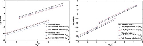
Figure 1 shows the optimal rate of convergence for dG(0)-cG(1) and dG(1)-cG(1) with uniform in time $L_2$-norm for the displacement and the velocity, that is in agreement with (44(44) $\begin{array}{rl}\Vert e_1{\Vert }_{1,J_N}& +\Vert e_2{\Vert }_{J_N}\\ & \le C(k^{\mathrm{q}+1}\{\Vert u_1^{(\mathrm{q}+1)}{\Vert }_{1,J_N}+\Vert u_2^{(\mathrm{q}+1)}{\Vert }_{1,J_N}\}\\ & +\sum _{n=1}^N{k}_n^{\mathrm{q}+2}\{\Vert u_2^{(\mathrm{q}+1)}{\Vert }_{1,I_n}+\Vert u_1^{(\mathrm{q}+1)}{\Vert }_{2,I_n}\}\\ & +h^{\mathrm{r}}\{\Vert v_0{\Vert }_{\mathrm{r}}+{\int }_0^T\Vert {\dot{u}}_2{\Vert }_{\mathrm{r}}\mathrm{d}t+\Vert u_1{\Vert }_{\mathrm{r}+1,J_N}+\Vert u_2{\Vert }_{\mathrm{r},J_N}\}),\end{array}$(44) ) and (45(45) $\begin{array}{rl}& \Vert e_1{\Vert }_{J_N}\le C(k^{\mathrm{q}+1}\Vert u_1^{(\mathrm{q}+1)}{\Vert }_{1,J_N}+\sum _{n=1}^N{k}_n^{\mathrm{q}+2}\{\Vert u_2^{(\mathrm{q}+1)}{\Vert }_{I_n}+\Vert u_1^{(\mathrm{q}+1)}{\Vert }_{1,I_n}\}\\ & +h^{\mathrm{r}+1}\{{\int }_0^T\Vert u_2{\Vert }_{\mathrm{r}+1}\mathrm{d}t+\Vert u_1{\Vert }_{\mathrm{r}+1,J_N}\}).\end{array}$(45) ). We have used short time T = 1 and long time T = 10. The figures for the error estimates (39(39) $\begin{array}{rl}& \Vert e_{1,N}^{-}{\Vert }_1+\Vert e_{2,N}^{-}\Vert \le C(\sum _{n=1}^N{k}_n^{\mathrm{q}+1}{\int }_{I_n}\{\Vert u_2^{(\mathrm{q}+1)}{\Vert }_1+\Vert u_1^{(\mathrm{q}+1)}{\Vert }_2\}\mathrm{d}t\\ & +h^{\mathrm{r}}\{\Vert v_0{\Vert }_{\mathrm{r}}+{\int }_0^T\Vert {\dot{u}}_2{\Vert }_{\mathrm{r}}\mathrm{d}t+\Vert u_{1,N}{\Vert }_{\mathrm{r}+1}+\Vert u_{2,N}{\Vert }_{\mathrm{r}}\}),\end{array}$(39) ) and (40(40) $\begin{array}{rl}& \Vert e_{1,N}^{-}\Vert \le C(\sum _{n=1}^N{k}_n^{\mathrm{q}+1}{\int }_{I_n}\{\Vert u_2^{(\mathrm{q}+1)}\Vert +\Vert u_1^{(\mathrm{q}+1)}{\Vert }_1\}\mathrm{d}t\\ & +h^{\mathrm{r}+1}\{{\int }_0^T\Vert u_2{\Vert }_{\mathrm{r}+1}\mathrm{d}t+\Vert u_{1,N}{\Vert }_{\mathrm{r}+1}\}).\end{array}$(40) ) are very similar, as expected, and therefore they are not presented here.

Figure 1. Temporal rate of convergence with uniform in time $L^2$-norm for the displacement and the velocity, with T = 1, 10: (left) dG(0) (right) dG(1).

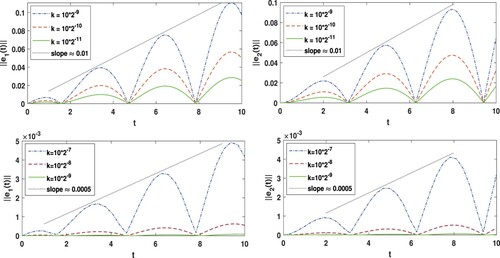
The behaviour of the errors $\Vert e_1\left(t\right)\Vert$ and $\Vert e_2\left(t\right)\Vert$ in time are shown in Figure 2 for both dG(0) and dG(1), with T = 10. We note that the slope of error accumulation is very small, in particular, for dG(1) in compare with the finest time mesh $10\ast 2^{-9}$. This shows that the error accumulation does not depend on time T in long-time integration, since the stability constants are independent of T.

Figure 2. Behaviour of the errors $\Vert e_1\left(t\right)\Vert$ and $\Vert e_2\left(t\right)\Vert$ in time: (up) dG(0) (down) dG(1).

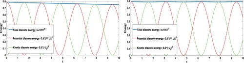
The total energy of the system is $\frac{1}{2}\Vert \mathrm{\nabla }u{\Vert }^2+\frac{1}{2}\Vert \dot{u}{\Vert }^2=\frac{\pi }{4}$. The discrete energy (for three different time steps) has been compared with the theoretical energy in Figure 3, for both methods dG(0) and dG(1). In Figure 4, we show the discrete energy for dG(0) with the time step $k=10\cdot 2^{-9}$, and for dG(1) with even a bigger time step $k=10\cdot 2^{-7}$. In all experiments dG(1) outperforms dG(0). It is shown that dG(1) is much more accurate even with a considerably larger time step.

Figure 3. Comparison of the theoretical (continuous) energy and the discrete energy for different values of the time step k: (left) dG(0) (right) dG(1).

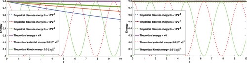
Figure 4. Discrete energy: (left) dG(0) with $k=10\cdot 2^{-9}$ (right) dG(1) with $k=10\cdot 2^{-7}$.

Acknowledgments

The authors would like to thank the anonymous referee for the constructive comments that helped us to improve the manuscript. The authors also thank Prof. Omar Lakkis for fruitful discussion and his constructive comments.

Disclosure statement

No potential conflict of interest was reported by the author(s).

References

- S. Adjerid and H. Temimi, A discontinuous Galerkin method for the wave equation, Comput. Methods Appl. Mech. Eng. 200 (2011), pp. 837–849.
- G.A. Baker, Error estimates for finite element methods for second order hyperbolic equations, SIAM J. Numer. Anal. 13 (1976), pp. 564–576.
- L. Banjai, E.H. Georgoulis, and O. Lijoka, A Trefftz polynomial space-time discontinuous Galerkin method for the second order wave equation, SIAM J. Numer. Anal. 55 (2017), pp. 63–86.
- P. Castillo, A superconvergence result for discontinuous Galerkin methods applied to elliptic problems, Comput. Methods Appl. Mech. Eng. 192 (2003), pp. 4675–4685.
- F. Celiker and B. Cockburn, Superconvergence of the numerical traces for discontinuous Galerkin and hybridized methods for convection-diffusion problems in one space dimension, Math. Comput. 76 (2007), pp. 67–96.
- M. Delfour, W. Hager, and F. Trochu, Discontinuous Galerkin methods for ordinary differential equations, Math. Comp. 36 (1981), pp. 455–473.
- T. Dupont, L2-estimates for Galerkin methods for second order hyperbolic equations, SIAM J. Numer. Anal. 10 (1973), pp. 880–889.
- K. Eriksson and C. Johnson, Adaptive finite element methods for parabolic problems I: A linear model problem, SIAM J. Numer. Anal. 28 (1991), pp. 43–77.
- K. Eriksson, C. Johnson, and S. Larsson, Adaptive finite element methods for parabolic problems IV: analytic semigroups, SIAM J. Numer. Anal. 35 (1998), pp. 1315–1325.
- K. Eriksson, C. Johnson, and V. Thomée, Time discretization of parabolic problems by the discontinuous Galerkin method, RAIRO Modél. Math. Anal. Numér. 19 (1985), pp. 611–643.
- D.A. French and T.E. Peterson, A continuous space-time finite element method for the wave equation, Math. Comput. 65 (1996), pp. 491–506.
- M.J. Grote, A. Schneebeli, and D. Schötzau, Discontinuous Galerkin finite element method for the wave equation, SIAM J. Numer. Anal. 6 (2006), pp. 2408–2431.
- C. Johnson, Error estimates and adaptive time-step control for a class of one-step methods for stiff ordinary differential equations, SIAM J. Numer. Anal. 25 (1988), pp. 908–926.
- C. Johnson, Discontinuous finite element for second-order hyperbolic problems, Comput. Methods Appl. Mech. Eng. 107 (1993), pp. 117–129.
- M. Kovács, S. Larsson, and F. Saedpanah, Finite element approximation for the linear stochastic wave equation with additive noise, SIAM J. Numer. Anal. 48 (2010), pp. 408–427.
- S. Larsson, M. Racheva, and F. Saedpanah, Discontinuous Galerkin method for an integro-differential equation modeling dynamic fractional order viscoelasticity, Comput. Methods Appl. Mech. Eng. 283 (2015), pp. 196–209.
- S. Larsson and F. Saedpanah, The continuous Galerkin method for an integro-differential equation modeling dynamic fractional order viscoelasticity, IMA J. Numer. Anal. 30 (2010), pp. 964–986.
- S. Larsson, V. Thomée, and L.B. Wahlbin, Numerical solution of parabolic integro-differential equations by the discontinuous Galerkin method, Math. Comp. 67 (1998), pp. 45–71.
- P. Lasaint and P.A. Raviart, On a finite element method for solving the neutron transport equation, in Mathematical Aspects of Finite Elements in Partial Differential Equations, Academic Press, New York, 1974, pp. 89–123.
- F. Müller, D. Schötzau, and Ch. Schwab, Discontinuous Galerkin methods for acoustic wave propagation in polygons, J. Sci. Comput. 77 (2018), pp. 1909–1935.
- K. Mustapha and W. Mclean, Discontinuous Galerkin method for an evolution equation with a memory term of positive type, Math. Comput. 78 (2009), pp. 1975–1995.
- A. Quarteroni and A. Valli, Numerical Approximation of Partial Differential Equations, Springer-Verlag, Berlin and Heidelberg, 1994.
- J. Rauch, On convergence of the finite element method for the wave equation, SIAM J. Numer. Anal.22 (1985), pp. 245–249.
- W. Reed and T. Hill, Triangular Mesh Methods for the Neutron Transport Equation, Technical Report LA- UR-73-479, Los Alamos Scientific Laboratory, Los Alamos, NM, 1973.
- B. Riviere and M. Wheeler, Discontinuous finite element methods for acoustic and elastic wave problems, Contemp. Math. 329 (2003), pp. 271–282.
- F. Saedpanah, Continuous Galerkin finite element methods for hyperbolic integro-differential equations, IMA J. Numer. Anal. 35 (2015), pp. 885–908.
- L. Schmutz and T.P. Wihler, The variable-order discontinuous Galerkin time stepping scheme for parabolic evolution problems is uniformly L∞-stable, SIAM J. Numer. Anal. 57 (2019), pp. 293–319.
- V. Thomée, Galerkin Finite Element Methods for Parabolic Problems, Springer- Verlag, Berlin, 2006.