Estimating stresses driving tissue flows using a stokes inverse problem

ABSTRACT

We propose an inverse problem to derive the stress distributions that drive the tissue flows during gastrulation in the epiblast of the chick embryo, from measurements of the tissue velocity fields at different stages of development. We assume that the embryonic tissue can be described as a highly viscous fluid, characterized by the Stokes equations. Using the theory of the optimal control, the stress distributions are determined by minimizing an objective functional, which is constructed such that it can match the numerical velocity of the flow with the experimental velocity data by choosing the stress as the control variable. The Lagrange multiplier method is utilized to derive the optimality system. The finite element method is used to approximate these partial differential equations numerically and we use the conjugate gradient algorithm to solve the optimal control problem.

KEYWORDS:

• Stokes equation
• inverse problem
• optimal control model
• chick embryo gastrulation
• conjugate gradient method

MSC2020 AMS SUBJECT CLASSIFICATION:

• 68Q07

1. Introduction

One of the earliest stages in embryogenesis is gastrulation, which is a critical stage in the development of all higher organisms. During gastrulation, three germ layers, i.e. ectoderm, mesoderm and endoderm, will form and assume their definitive positions in the embryo [26]. Cell and tissue movements play an essential role in the development of multicellular organisms, especially during gastrulation, formation of the nervous system and organogenesis. When not properly controlled, it results in severe defects and diseases. It is thus very important to understand the movement mechanisms that drive gastrulation.

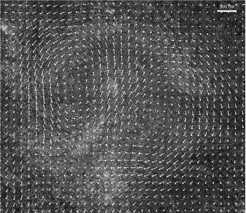
The chick embryo is a well established model organism for investigation of amniote gastrulation, including humans, since it is essentially flat, transparent and develops outside the mother [31,32]. In the chick embryo, gastrulation starts with the formation of the primitive streak, which involves large-scale cell flows of more than 100,000 cells. During the primitive streak formation, the epiblast cells are moving as two vortical cellular flows along the midline of the embryo, from the posterior position to the anterior position and are replaced by cells moving in from more lateral positions (Figure 1) [2,5]. These vortices rotate in opposite directions-away from the midline in the anterior and towards the midline in the posterior. When the cell flows meet at the posterior of the epiblast, the cells start to stack on top of each other and the epiblast becomes several cell-layers thick, forming a structure macroscopically visible as the primitive streak and the future mesendoderm and endoderm [3,4,23,27,32,33].

Figure 1. Particle Image Velocimetry (PIV) of cell flow velocity fields in epiblast of chicken embryo during primitive streak formation Figure Credit: C.J. Weijer Lab. White arrows show direction of tissue flow. The white scale bar is 300 $\mu$m in length and $4\mu \mathrm{m}{\min }^{-1}$ in tissue velocity.

Improved experimental methods have been developed that enable us to analyse the large-scale vortical cellular flow patterns under normal and experimentally perturbed conditions with high precision [5,21,29]. However, the stress distributions that drive these tissue flows during chick gastrulation are difficult to be measured directly. We assume that the large-scale tissue flows during gastrulation in chick embryos satisfy Stokes equations [3,4,22,23,27,33]. To calculate the stress distributions driving these tissue flows, we propose to use a combination of mathematical modelling and computational techniques to infer these stress distributions from experimentally measured velocity fields by solving an inverse and optimal control problem [13]. We will choose the stress as the control variable and construct an objective functional that will allow us to match the numerical velocities for an optimal stress distribution with the experimentally measured flow velocity data. The optimal stress distribution will be determined by minimizing this objective functional.

We will consider the following non-stationary incompressible Stokes equations with Dirichlet boundary condition: (1) $\{\begin{array}{ll}{\mathbf{u}}_t-\mu △\mathbf{u}+▽\mathit{p}\mathit{=}\mathbf{f}\mathit{,}& \mathrm{in}\mathrm{\Omega }\times (0,T],\\ ▽\cdot \mathbf{u}=0,& \mathrm{in}\mathrm{\Omega }\times [0,T],\\ \mathbf{u}{\mid }_{\mathrm{\Gamma }}=\mathbf{a},\mathbf{u}{\mid }_{t=0}=\mathbf{b},& \end{array}$(1) where $\mathrm{\Omega }\subset {\mathbf{R}}^2$ is a bounded domain with boundary Γ and $[0,T]$ is a time interval. Here, $\mathbf{u}(\mathbf{x},t)$ represents the velocity of the cellular flows, $\mathit{p}\mathit{(}\mathbf{x}\mathit{,}\mathit{t}\mathit{)}$ denotes the pressure, $\mathbf{f}(\mathbf{x},t)$ is the stress acting on the tissue, μ is the dynamic viscosity, $\mathbf{a}(\mathbf{x},t)$ and $\mathbf{b}(\mathbf{x})$ are given values on the boundary Γ and the initial time, respectively. $▽\cdot \mathbf{u}=0$ means the fluid is incompressible (divergence-free). In this problem, the experimental velocity fields and domain are recorded by the particle image velocimetry (PIV). PIV provides information about the local velocity of small approximately cell-sized tissue regions and allows calculation of detailed local spatiotemporal movement of these tissue domains over time [21]. One frame of the PIV in one chick embryo during the early stages of primitive streak formation (stage HH2) is shown in Figure 1.

2. Optimal control model

2.1. Objective functional

Our target is to determine proper stress distributions $\mathbf{f}$ so that the numerical velocity fields will match the experiment data, hence we can present the following objective functional (2) $J_1(\mathbf{u},\mathbf{f})=\frac{1}{2}{\int }_0^T{\int }_{\mathrm{\Omega }}|\mathbf{u}-\overline{\mathbf{u}}{|}^2\mathrm{d}\mathbf{x}\mathrm{d}t,$(2) where $|\mathbf{u}{|}^2=\mathbf{u}\cdot \mathbf{u}=\sum _{i=1}^2{u}_i^2$. $\overline{\mathbf{u}}(\mathbf{x},t)$ denotes the experiment velocity at location $(x,y)$ and time t in chick embryo, while $\mathbf{u}(\mathbf{x},t)$ represents for the numerical velocity. While problem (2(2) $J_1(\mathbf{u},\mathbf{f})=\frac{1}{2}{\int }_0^T{\int }_{\mathrm{\Omega }}|\mathbf{u}-\overline{\mathbf{u}}{|}^2\mathrm{d}\mathbf{x}\mathrm{d}t,$(2) ) is ill-posed, a standard method to improve the smoothness of the flow and make the problem well-posed is to add a variational term [1,9,20]. In this case, as we need to confine $\mathbf{u}$ to Stokes system, we choose the standard form of the control variable to be $\mathbf{f}$, which is often used in dealing with the ill-posed problem and avoid multiple solutions [10]. Therefore, the objective functional becomes (3) $J(\mathbf{u},\mathbf{f})=\frac{1}{2}{\int }_0^T{\int }_{\mathrm{\Omega }}|\mathbf{u}-\overline{\mathbf{u}}{|}^2\mathrm{d}\mathbf{x}\mathrm{d}t+\frac{\alpha }{2}{\int }_0^T{\int }_{\mathrm{\Omega }}|\mathbf{f}{|}^2\mathrm{d}\mathbf{x}\mathrm{d}t,$(3) where, α is a positive constant measuring the importance between two terms in $J(\mathbf{u},\mathbf{f})$. Hence the optimal control problem is to find a suitable control variable $\mathbf{f}$ to minimize $J(\mathbf{u},\mathbf{f})$, where variables $\mathbf{u}$ and $\mathbf{f}$ are subject to Stokes equations (1(1) $\{\begin{array}{ll}{\mathbf{u}}_t-\mu △\mathbf{u}+▽\mathit{p}\mathit{=}\mathbf{f}\mathit{,}& \mathrm{in}\mathrm{\Omega }\times (0,T],\\ ▽\cdot \mathbf{u}=0,& \mathrm{in}\mathrm{\Omega }\times [0,T],\\ \mathbf{u}{\mid }_{\mathrm{\Gamma }}=\mathbf{a},\mathbf{u}{\mid }_{t=0}=\mathbf{b},& \end{array}$(1) ). To show the existence and uniqueness result of the optimal control problem, we cite the following Theorem 2.1 [30].

Theorem 2.1

Let $\{U,\Vert \cdot {\Vert }_U\}$ and $\{H,\Vert \cdot {\Vert }_H\}$ denote real Hilbert spaces, and let some $y_d\in H$ and constant $\alpha >0$ be given. Moreover, let $S:U\to H$ be a continuous linear operator. Then the quadratic Hilbert space optimization problem (4) $\underset{u\in U}{min}J(u):=\frac{1}{2}{\Vert Su-y_d\Vert }_H^2+\frac{\alpha }{2}{\Vert u\Vert }_U^2$(4) admits a unique optimal solution.

For the optimal control problem (3(3) $J(\mathbf{u},\mathbf{f})=\frac{1}{2}{\int }_0^T{\int }_{\mathrm{\Omega }}|\mathbf{u}-\overline{\mathbf{u}}{|}^2\mathrm{d}\mathbf{x}\mathrm{d}t+\frac{\alpha }{2}{\int }_0^T{\int }_{\mathrm{\Omega }}|\mathbf{f}{|}^2\mathrm{d}\mathbf{x}\mathrm{d}t,$(3) , 1(1) $\{\begin{array}{ll}{\mathbf{u}}_t-\mu △\mathbf{u}+▽\mathit{p}\mathit{=}\mathbf{f}\mathit{,}& \mathrm{in}\mathrm{\Omega }\times (0,T],\\ ▽\cdot \mathbf{u}=0,& \mathrm{in}\mathrm{\Omega }\times [0,T],\\ \mathbf{u}{\mid }_{\mathrm{\Gamma }}=\mathbf{a},\mathbf{u}{\mid }_{t=0}=\mathbf{b},& \end{array}$(1) ), we denote the space-time cylinder $Q=\mathrm{\Omega }\times (0,T)$ and give functions $\mathbf{f}\in (L^2(Q){)}^2$, there is a continuous linear mapping regarding to Stokes equations (1(1) $\{\begin{array}{ll}{\mathbf{u}}_t-\mu △\mathbf{u}+▽\mathit{p}\mathit{=}\mathbf{f}\mathit{,}& \mathrm{in}\mathrm{\Omega }\times (0,T],\\ ▽\cdot \mathbf{u}=0,& \mathrm{in}\mathrm{\Omega }\times [0,T],\\ \mathbf{u}{\mid }_{\mathrm{\Gamma }}=\mathbf{a},\mathbf{u}{\mid }_{t=0}=\mathbf{b},& \end{array}$(1) ): (5) $S:(L^2(Q){)}^2\to (L^2(Q){)}^2,\mathbf{f}\mapsto \mathbf{\text{u}}.$(5) Replacing $\mathbf{\text{u}}$ in the objective functional (3(3) $J(\mathbf{u},\mathbf{f})=\frac{1}{2}{\int }_0^T{\int }_{\mathrm{\Omega }}|\mathbf{u}-\overline{\mathbf{u}}{|}^2\mathrm{d}\mathbf{x}\mathrm{d}t+\frac{\alpha }{2}{\int }_0^T{\int }_{\mathrm{\Omega }}|\mathbf{f}{|}^2\mathrm{d}\mathbf{x}\mathrm{d}t,$(3) ) by $S\mathbf{\text{f}}$, the optimal control problem (3(3) $J(\mathbf{u},\mathbf{f})=\frac{1}{2}{\int }_0^T{\int }_{\mathrm{\Omega }}|\mathbf{u}-\overline{\mathbf{u}}{|}^2\mathrm{d}\mathbf{x}\mathrm{d}t+\frac{\alpha }{2}{\int }_0^T{\int }_{\mathrm{\Omega }}|\mathbf{f}{|}^2\mathrm{d}\mathbf{x}\mathrm{d}t,$(3) , 1(1) $\{\begin{array}{ll}{\mathbf{u}}_t-\mu △\mathbf{u}+▽\mathit{p}\mathit{=}\mathbf{f}\mathit{,}& \mathrm{in}\mathrm{\Omega }\times (0,T],\\ ▽\cdot \mathbf{u}=0,& \mathrm{in}\mathrm{\Omega }\times [0,T],\\ \mathbf{u}{\mid }_{\mathrm{\Gamma }}=\mathbf{a},\mathbf{u}{\mid }_{t=0}=\mathbf{b},& \end{array}$(1) ) reduces to the following quadratic optimization problem: (6) $\underset{\mathbf{\text{f}}\in (L^2(Q){)}^2}{min}J(\mathbf{\text{f}}):=\frac{1}{2}{\Vert S\mathbf{\text{f}}-\overline{\mathbf{\text{u}}}\Vert }_{(L^2(Q){)}^2}^2+\frac{\alpha }{2}{\Vert \mathbf{\text{f}}\Vert }_{(L^2(Q){)}^2}^2$(6) The functional J is convex and continuous and $\alpha >0$, hence, the optimal control problem (6(6) $\underset{\mathbf{\text{f}}\in (L^2(Q){)}^2}{min}J(\mathbf{\text{f}}):=\frac{1}{2}{\Vert S\mathbf{\text{f}}-\overline{\mathbf{\text{u}}}\Vert }_{(L^2(Q){)}^2}^2+\frac{\alpha }{2}{\Vert \mathbf{\text{f}}\Vert }_{(L^2(Q){)}^2}^2$(6) ) has a unique optimal solution inferred from Theorem 2.1.

2.2. Optimality system

To derive the optimal solutions of (3(3) $J(\mathbf{u},\mathbf{f})=\frac{1}{2}{\int }_0^T{\int }_{\mathrm{\Omega }}|\mathbf{u}-\overline{\mathbf{u}}{|}^2\mathrm{d}\mathbf{x}\mathrm{d}t+\frac{\alpha }{2}{\int }_0^T{\int }_{\mathrm{\Omega }}|\mathbf{f}{|}^2\mathrm{d}\mathbf{x}\mathrm{d}t,$(3) ), we should build the optimality system by the optimal control theory. The optimality system consists of the state equations, the adjoint equations and the optimality condition. We utilize a general Lagrange multiplier existence result in order to derive an appropriate optimality system for the control problem.

By introducing the Lagrange multipliers $\mathbf{v},q$ on $\mathrm{\Omega }\times (0,T)$, we set up the Lagrange functional (7) $L(\mathbf{u},p,\mathbf{f},\mathbf{v},q)=J(\mathbf{u},\mathbf{f})-{\int }_0^T{\int }_{\mathrm{\Omega }}\{\mathbf{v}\cdot ({\mathbf{u}}_t-\mu △\mathbf{u}+▽\mathit{p}\mathit{-}\mathbf{\text{f}}\mathit{)}\mathit{+}\mathit{q}\mathit{(}▽\cdot \mathbf{u}\mathit{)}\}\mathrm{d}\mathbf{x}\mathrm{d}\mathit{t}\mathit{,}$(7) As first order approximation the optimality system can be derived by taking G$\hat{a}$teaux derivative of $L(\mathbf{u},p,\mathbf{f},\mathbf{v},q)$ with respect to the variables $\{\mathbf{u},p\}$, the Lagrange multipliers $\{\mathbf{v},q\}$ and the control variable $\mathbf{f}$, respectively. The G$\hat{a}$teaux derivative of $L(\mathbf{u},p,\mathbf{f},\mathbf{v},q)$ with respect to the variables $\{\mathbf{u},p,\mathbf{v},q,\mathbf{f}$} exist as there is an operator $A:U\to V$, where U, V are Banach spaces, such that (8) $\underset{t\downarrow 0}{lim}\frac{1}{t}(L(u+th)-L(u))=⟨A,h⟩,\mathrm{\forall }h\in U.$(8) A is referred to as the G$\hat{a}$teaux derivative of L at u.

State equations. To derive the state equations, we differentiate $L(\mathbf{u},p,\mathbf{f},\mathbf{v},q)$ with respect to the Lagrange multiplier $\mathbf{v}$ to obtain (9) $⟨\frac{\delta L}{\delta \mathbf{v}},{\mathbf{v}}^0⟩=\frac{\mathrm{d}L(\mathbf{u},p,\mathbf{f},\mathbf{v}+ϵ{\mathbf{v}}^0,q)}{\mathrm{d}ϵ}{|}_{ϵ=0}=0,$(9) i.e. (10) $⟨\frac{\delta L}{\delta \mathbf{v}},{\mathbf{v}}^0⟩=-{\int }_0^T{\int }_{\mathrm{\Omega }}{\mathbf{v}}^0\cdot ({\mathbf{u}}_t-\mu △\mathbf{u}+▽\mathit{p}\mathit{-}\mathbf{\text{f}}\mathit{)}\mathrm{d}\mathbf{x}\mathrm{d}\mathit{t}\mathit{=}\mathit{0.}$(10) Noticing that ${\mathbf{v}}^0$ is chosen arbitrarily, we formally have (11) $\frac{\delta L}{\delta \mathbf{v}}={\mathbf{u}}_t-\mu △\mathbf{u}+▽\mathit{p}\mathit{-}\mathbf{\text{f}}\mathit{=}\mathit{0.}$(11) Similarly to the Lagrange multiplier q, we have (12) $\frac{\delta L}{\delta q}=▽\cdot \mathbf{u}=0.$(12) We assume that $\mathbf{u}$ is equal to $\overline{\mathbf{u}}$ on the boundary, and take the initial condition to be 0. Therefore, from (11(11) $\frac{\delta L}{\delta \mathbf{v}}={\mathbf{u}}_t-\mu △\mathbf{u}+▽\mathit{p}\mathit{-}\mathbf{\text{f}}\mathit{=}\mathit{0.}$(11) ) and (12(12) $\frac{\delta L}{\delta q}=▽\cdot \mathbf{u}=0.$(12) ), the state equations become (13) $\{\begin{array}{ll}{\mathbf{u}}_t-\mu △\mathbf{u}+▽\mathit{p}\mathit{=}\mathbf{f}\mathit{,}& \mathrm{in}\mathrm{\Omega }\times (0,T],\\ ▽\cdot \mathbf{u}=0,& \mathrm{in}\mathrm{\Omega }\times [0,T],\\ \mathbf{u}{|}_{\mathrm{\Gamma }}=\overline{\mathbf{u}}{|}_{\mathrm{\Gamma }},\mathbf{u}{|}_{t=0}=\mathbf{0}.& \end{array}$(13) Adjoint equations. To derive the adjoint equations, we differentiate $L(\mathbf{u},p,\mathbf{f},\mathbf{v},q)$ with respect to $\mathbf{u}$ to have (14) $⟨\frac{\delta L}{\delta \mathbf{u}},{\mathbf{u}}^0⟩=\frac{\mathrm{d}L(\mathbf{u}+ϵ{\mathbf{u}}^0,p,\mathbf{f},\mathbf{v},q)}{\mathrm{d}ϵ}{|}_{ϵ=0}=0,$(14) where ${\mathbf{u}}^0$ is arbitrary and satisfies the conditions ${\mathbf{u}}^0{\mid }_{\mathrm{\Gamma }}=0,{\mathbf{u}}^0{\mid }_{t=0}=\mathbf{0}.$

Using the definition of the Lagrange functional (7(7) $L(\mathbf{u},p,\mathbf{f},\mathbf{v},q)=J(\mathbf{u},\mathbf{f})-{\int }_0^T{\int }_{\mathrm{\Omega }}\{\mathbf{v}\cdot ({\mathbf{u}}_t-\mu △\mathbf{u}+▽\mathit{p}\mathit{-}\mathbf{\text{f}}\mathit{)}\mathit{+}\mathit{q}\mathit{(}▽\cdot \mathbf{u}\mathit{)}\}\mathrm{d}\mathbf{x}\mathrm{d}\mathit{t}\mathit{,}$(7) ), we calculate (14(14) $⟨\frac{\delta L}{\delta \mathbf{u}},{\mathbf{u}}^0⟩=\frac{\mathrm{d}L(\mathbf{u}+ϵ{\mathbf{u}}^0,p,\mathbf{f},\mathbf{v},q)}{\mathrm{d}ϵ}{|}_{ϵ=0}=0,$(14) ) term by term. (i): It is easy to see that (15) $\frac{\mathrm{d}}{\mathrm{d}ϵ}\left(\frac{1}{2}{\int }_0^T{\int }_{\mathrm{\Omega }}|\mathbf{u}+ϵ{\mathbf{u}}^0-\overline{\mathbf{u}}{|}^2\mathrm{d}\mathbf{x}\mathrm{d}t\right){|}_{ϵ=0}={\int }_0^T{\int }_{\mathrm{\Omega }}{\mathbf{u}}^0\cdot (\mathbf{u}-\overline{\mathbf{u}})\mathrm{d}\mathbf{x}\mathrm{d}t.$(15) (ii): By integration by parts, we find (16) $\begin{array}{rl}& {\int }_0^T{\int }_{\mathrm{\Omega }}\mathbf{v}\cdot {\mathbf{u}}_t^0\mathrm{d}\mathbf{x}\mathrm{d}t={\int }_0^T{\int }_{\mathrm{\Omega }}[({\mathbf{u}}^0\cdot \mathbf{v}{)}_t-{\mathbf{u}}^0\cdot {\mathbf{v}}_t]\mathrm{d}\mathbf{x}\mathrm{d}t\\ & ={\int }_{\mathrm{\Omega }}[({\mathbf{u}}^0\cdot \mathbf{v}{)}_{t=T}-({\mathbf{u}}^0\cdot \mathbf{v}{)}_{t=0}]\mathrm{d}\mathbf{x}+{\int }_0^T{\int }_{\mathrm{\Omega }}[-{\mathbf{u}}^0\cdot {\mathbf{v}}_t]\mathrm{d}\mathbf{x}\mathrm{d}t.\end{array}$(16) Since ${\mathbf{u}}^0{\mid }_{t=0}=\mathbf{0}$ and if we let $\mathbf{v}{\mid }_{t=T}=\mathbf{0}$, we have (17) ${\int }_0^T{\int }_{\mathrm{\Omega }}\mathbf{v}\cdot {\mathbf{u}}_t^0\mathrm{d}\mathbf{x}\mathrm{d}t=-{\int }_0^T{\int }_{\mathrm{\Omega }}{\mathbf{u}}^0\cdot {\mathbf{v}}_t\mathrm{d}\mathbf{x}\mathrm{d}t.$(17) (iii): Similarly, we derive $\begin{array}{rl}{\int }_0^T{\int }_{\mathrm{\Omega }}\mathbf{v}\cdot (-\mu △{\mathbf{u}}^0)\mathrm{d}\mathbf{x}\mathrm{d}t& =-\mu {\int }_0^T{\int }_{\mathrm{\Omega }}[▽\cdot ((\mathbf{v}\cdot ▽){\mathbf{u}}^0)-▽\mathbf{v}:▽{\mathbf{u}}^0]\mathrm{d}\mathbf{x}\mathrm{d}t\\ & =-\mu {\int }_0^T{\int }_{\mathrm{\Gamma }}((\mathbf{v}\cdot ▽){\mathbf{u}}^0)\cdot \mathbf{n}\mathrm{d}s\mathrm{d}t+\mu {\int }_0^T{\int }_{\mathrm{\Omega }}▽\mathbf{v}:▽{\mathbf{u}}^0\mathrm{d}\mathbf{x}\mathrm{d}t,\end{array}$where $\mathbf{n}$ is the unit vector outward normal to Γ. Since ${\mathbf{u}}^0$ is equal to 0 on the boundary and if we set $\mathbf{v}$ is equal to 0 on the boundary, we have (18) $\begin{array}{rl}{\int }_0^T{\int }_{\mathrm{\Omega }}\mathbf{v}\cdot (-\mu △{\mathbf{u}}^0)\mathrm{d}\mathbf{x}\mathrm{d}t& =\mu {\int }_0^T{\int }_{\mathrm{\Omega }}▽\mathbf{v}:▽{\mathbf{u}}^0\mathrm{d}\mathbf{x}\mathrm{d}t\\ & =\mu {\int }_0^T{\int }_{\mathrm{\Omega }}[▽\cdot (({\mathbf{u}}^0\cdot ▽)\mathbf{v})-{\mathbf{u}}^0\cdot △\mathbf{v}]\mathrm{d}\mathbf{x}\mathrm{d}t\\ & =\mu {\int }_0^T{\int }_{\mathrm{\Gamma }}((\mathbf{v}\cdot ▽){\mathbf{u}}^0)\cdot \mathbf{n}\mathrm{d}s\mathrm{d}t-\mu {\int }_0^T{\int }_{\mathrm{\Omega }}{\mathbf{u}}^0\cdot △\mathbf{v}\mathrm{d}\mathbf{x}\mathrm{d}t\\ & =-\mu {\int }_0^T{\int }_{\mathrm{\Omega }}{\mathbf{u}}^0\cdot △\mathbf{v}\mathrm{d}\mathbf{x}\mathrm{d}t.\end{array}$(18) (iv): Finally, we have (19) ${\int }_0^T{\int }_{\mathrm{\Omega }}q(▽\cdot {\mathbf{u}}^0)\mathrm{d}\mathbf{x}\mathrm{d}t=-{\int }_0^T{\int }_{\mathrm{\Omega }}{\mathbf{u}}^0\cdot (▽q)\mathrm{d}\mathbf{x}\mathrm{d}t.$(19) Collecting Equations (15(15) $\frac{\mathrm{d}}{\mathrm{d}ϵ}\left(\frac{1}{2}{\int }_0^T{\int }_{\mathrm{\Omega }}|\mathbf{u}+ϵ{\mathbf{u}}^0-\overline{\mathbf{u}}{|}^2\mathrm{d}\mathbf{x}\mathrm{d}t\right){|}_{ϵ=0}={\int }_0^T{\int }_{\mathrm{\Omega }}{\mathbf{u}}^0\cdot (\mathbf{u}-\overline{\mathbf{u}})\mathrm{d}\mathbf{x}\mathrm{d}t.$(15) )–(19(19) ${\int }_0^T{\int }_{\mathrm{\Omega }}q(▽\cdot {\mathbf{u}}^0)\mathrm{d}\mathbf{x}\mathrm{d}t=-{\int }_0^T{\int }_{\mathrm{\Omega }}{\mathbf{u}}^0\cdot (▽q)\mathrm{d}\mathbf{x}\mathrm{d}t.$(19) ) together and noticing that ${\mathbf{u}}^0$ is chosen arbitrarily, we formally obtain (20) $\frac{\delta L}{\delta \mathbf{u}}={\mathbf{v}}_t+\mu △\mathbf{v}+▽\mathit{q}\mathit{+}\mathit{(}\mathbf{u}\mathit{-}\overline{\mathbf{u}}\mathit{)}\mathit{=}\mathit{0.}$(20) Similarly, the G$\hat{a}$teaux derivative of $L(\mathbf{u},p,\mathbf{f},\mathbf{v},q)$ with respect to p can be done to obtain (21) $\frac{\delta L}{\delta p}=▽\cdot \mathbf{v}=0.$(21) Finally, from (20(20) $\frac{\delta L}{\delta \mathbf{u}}={\mathbf{v}}_t+\mu △\mathbf{v}+▽\mathit{q}\mathit{+}\mathit{(}\mathbf{u}\mathit{-}\overline{\mathbf{u}}\mathit{)}\mathit{=}\mathit{0.}$(20) ) and (21(21) $\frac{\delta L}{\delta p}=▽\cdot \mathbf{v}=0.$(21) ), we have the adjoint equations (22) $\{\begin{array}{ll}-{\mathbf{v}}_t-\mu △\mathbf{v}-▽\mathit{q}\mathit{=}\mathbf{u}\mathit{-}\overline{\mathbf{u}}\mathit{,}& \mathrm{in}\mathrm{\Omega }\times [0,T),\\ ▽\cdot \mathbf{v}=0,& \mathrm{in}\mathrm{\Omega }\times [0,T],\\ \mathbf{v}{|}_{\mathrm{\Gamma }}=0,\mathbf{v}{|}_{t=T}=0.\end{array}$(22) Note that the adjoint Equation (22(22) $\{\begin{array}{ll}-{\mathbf{v}}_t-\mu △\mathbf{v}-▽\mathit{q}\mathit{=}\mathbf{u}\mathit{-}\overline{\mathbf{u}}\mathit{,}& \mathrm{in}\mathrm{\Omega }\times [0,T),\\ ▽\cdot \mathbf{v}=0,& \mathrm{in}\mathrm{\Omega }\times [0,T],\\ \mathbf{v}{|}_{\mathrm{\Gamma }}=0,\mathbf{v}{|}_{t=T}=0.\end{array}$(22) ) have the similar structures as the state Equation (13(13) $\{\begin{array}{ll}{\mathbf{u}}_t-\mu △\mathbf{u}+▽\mathit{p}\mathit{=}\mathbf{f}\mathit{,}& \mathrm{in}\mathrm{\Omega }\times (0,T],\\ ▽\cdot \mathbf{u}=0,& \mathrm{in}\mathrm{\Omega }\times [0,T],\\ \mathbf{u}{|}_{\mathrm{\Gamma }}=\overline{\mathbf{u}}{|}_{\mathrm{\Gamma }},\mathbf{u}{|}_{t=0}=\mathbf{0}.& \end{array}$(13) ) with the variables $\mathbf{u}$ and p replaced by the adjoint velocity v and the adjoint pressure $q$, respectively. Consequently, we can use the similar numerical algorithm to solve (13(13) $\{\begin{array}{ll}{\mathbf{u}}_t-\mu △\mathbf{u}+▽\mathit{p}\mathit{=}\mathbf{f}\mathit{,}& \mathrm{in}\mathrm{\Omega }\times (0,T],\\ ▽\cdot \mathbf{u}=0,& \mathrm{in}\mathrm{\Omega }\times [0,T],\\ \mathbf{u}{|}_{\mathrm{\Gamma }}=\overline{\mathbf{u}}{|}_{\mathrm{\Gamma }},\mathbf{u}{|}_{t=0}=\mathbf{0}.& \end{array}$(13) ) and (22(22) $\{\begin{array}{ll}-{\mathbf{v}}_t-\mu △\mathbf{v}-▽\mathit{q}\mathit{=}\mathbf{u}\mathit{-}\overline{\mathbf{u}}\mathit{,}& \mathrm{in}\mathrm{\Omega }\times [0,T),\\ ▽\cdot \mathbf{v}=0,& \mathrm{in}\mathrm{\Omega }\times [0,T],\\ \mathbf{v}{|}_{\mathrm{\Gamma }}=0,\mathbf{v}{|}_{t=T}=0.\end{array}$(22) ). Unlike the state Equation (13(13) $\{\begin{array}{ll}{\mathbf{u}}_t-\mu △\mathbf{u}+▽\mathit{p}\mathit{=}\mathbf{f}\mathit{,}& \mathrm{in}\mathrm{\Omega }\times (0,T],\\ ▽\cdot \mathbf{u}=0,& \mathrm{in}\mathrm{\Omega }\times [0,T],\\ \mathbf{u}{|}_{\mathrm{\Gamma }}=\overline{\mathbf{u}}{|}_{\mathrm{\Gamma }},\mathbf{u}{|}_{t=0}=\mathbf{0}.& \end{array}$(13) ) provided with an initial condition, the adjoint Equation (22(22) $\{\begin{array}{ll}-{\mathbf{v}}_t-\mu △\mathbf{v}-▽\mathit{q}\mathit{=}\mathbf{u}\mathit{-}\overline{\mathbf{u}}\mathit{,}& \mathrm{in}\mathrm{\Omega }\times [0,T),\\ ▽\cdot \mathbf{v}=0,& \mathrm{in}\mathrm{\Omega }\times [0,T],\\ \mathbf{v}{|}_{\mathrm{\Gamma }}=0,\mathbf{v}{|}_{t=T}=0.\end{array}$(22) ) are provided with a final condition at t = T. It can be solved conveniently by using the Backward-Euler difference in time.

The optimality condition. The optimality condition for optimal control problem is just the necessary condition of the functional $J(\mathbf{u},\mathbf{f})$ reaches its minimum values, i.e. that the G$\hat{a}$teaux derivative of $L(\mathbf{u},p,\mathbf{f},\mathbf{v},q)$ with respect to $\mathbf{f}$ vanishes at the optimum.

By differentiating $L(\mathbf{u},p,\mathbf{f},\mathbf{v},q)$ with respect to $\mathbf{f}$, we obtain (23) $⟨\frac{\delta L}{\delta \mathbf{f}},{\mathbf{f}}^0⟩=\frac{\mathrm{d}L(\mathbf{u},p,\mathbf{f}+ϵ{\mathbf{f}}^0,\mathbf{v},q)}{\mathrm{d}ϵ}{|}_{ϵ=0}=0,$(23) where ${\mathbf{f}}^0$ is arbitrary.

Calculating (23(23) $⟨\frac{\delta L}{\delta \mathbf{f}},{\mathbf{f}}^0⟩=\frac{\mathrm{d}L(\mathbf{u},p,\mathbf{f}+ϵ{\mathbf{f}}^0,\mathbf{v},q)}{\mathrm{d}ϵ}{|}_{ϵ=0}=0,$(23) ), we have (24) $⟨\frac{\delta L}{\delta \mathbf{f}},{\mathbf{f}}^0⟩={\int }_0^T{\int }_{\mathrm{\Omega }}(\alpha \mathbf{f}+\mathbf{v})\cdot {\mathbf{f}}^0\mathrm{d}\mathbf{x}\mathrm{d}t=0.$(24) Hence, the G$\hat{a}$teaux derivative of $L(\mathbf{u},p,\mathbf{f},\mathbf{v},q)$ with respect to $\mathbf{f}$ is (25) $\frac{\delta J}{\delta \mathbf{f}}=\mathbf{v}+\alpha \mathbf{f}.$(25) The optimality condition for optimal control problem is (26) $\mathbf{v}+\alpha \mathbf{f}=0,\mathrm{in}\mathrm{\Omega }\times (0,T).$(26) Now, we can present the full optimal control problem as the following optimality system: to find $\mathbf{u},p,\mathbf{f},\mathbf{v},\mathit{q}$ satisfy $\begin{array}{rl}& \{\begin{array}{ll}{\mathbf{u}}_t-\mu △\mathbf{u}+▽\mathit{p}\mathit{=}\mathbf{f}\mathit{,}& \mathrm{in}\mathrm{\Omega }\times (0,T],\\ ▽\cdot \mathbf{u}=0,& \mathrm{in}\mathrm{\Omega }\times [0,T],\\ \mathbf{u}{|}_{\mathrm{\Gamma }}=\overline{\mathbf{u}}{|}_{\mathrm{\Gamma }},\mathbf{u}{|}_{t=0}=\mathbf{0},& \end{array}\\ & \{\begin{array}{ll}-{\mathbf{v}}_t-\mu △\mathbf{v}-▽\mathit{q}\mathit{=}\mathbf{u}\mathit{-}\overline{\mathbf{u}}\mathit{,}& \mathrm{in}\mathrm{\Omega }\times [0,T),\\ ▽\cdot \mathbf{v}=0,& \mathrm{in}\mathrm{\Omega }\times [0,T],\\ \mathbf{v}{|}_{\mathrm{\Gamma }}=0,\mathbf{v}{|}_{t=T}=0,\end{array}\end{array}$and $\mathbf{v}+\alpha \mathbf{f}=0,\mathrm{in}\mathrm{\Omega }\times (0,T).$

3. Numerical approach

In this section, we consider the discretization and numerical solutions of the state Equation (13(13) $\{\begin{array}{ll}{\mathbf{u}}_t-\mu △\mathbf{u}+▽\mathit{p}\mathit{=}\mathbf{f}\mathit{,}& \mathrm{in}\mathrm{\Omega }\times (0,T],\\ ▽\cdot \mathbf{u}=0,& \mathrm{in}\mathrm{\Omega }\times [0,T],\\ \mathbf{u}{|}_{\mathrm{\Gamma }}=\overline{\mathbf{u}}{|}_{\mathrm{\Gamma }},\mathbf{u}{|}_{t=0}=\mathbf{0}.& \end{array}$(13) ) and the adjoint Equation (22(22) $\{\begin{array}{ll}-{\mathbf{v}}_t-\mu △\mathbf{v}-▽\mathit{q}\mathit{=}\mathbf{u}\mathit{-}\overline{\mathbf{u}}\mathit{,}& \mathrm{in}\mathrm{\Omega }\times [0,T),\\ ▽\cdot \mathbf{v}=0,& \mathrm{in}\mathrm{\Omega }\times [0,T],\\ \mathbf{v}{|}_{\mathrm{\Gamma }}=0,\mathbf{v}{|}_{t=T}=0.\end{array}$(22) ) in detail.

3.1. Finite element approximation

To discretize the state and adjoint equations, we use the finite element method. We set spaces (27) $U=(H_0^1(\mathrm{\Omega }){)}^2,W=\{q\in L^2(\mathrm{\Omega })|{\int }_{\mathrm{\Omega }}q=0\}.$(27) Multiplication of the first equation in (13(13) $\{\begin{array}{ll}{\mathbf{u}}_t-\mu △\mathbf{u}+▽\mathit{p}\mathit{=}\mathbf{f}\mathit{,}& \mathrm{in}\mathrm{\Omega }\times (0,T],\\ ▽\cdot \mathbf{u}=0,& \mathrm{in}\mathrm{\Omega }\times [0,T],\\ \mathbf{u}{|}_{\mathrm{\Gamma }}=\overline{\mathbf{u}}{|}_{\mathrm{\Gamma }},\mathbf{u}{|}_{t=0}=\mathbf{0}.& \end{array}$(13) ) with $\tilde{\mathbf{u}}\in U$ and the second equation with $\tilde{p}\in W$, integrating over Ω and applying Green's formula, yields the weak form with the inner product $(\mathbf{\text{f}},\mathbf{\text{g}})={\int }_{\mathrm{\Omega }}\mathbf{\text{f}}\cdot \mathbf{\text{g}}d\mathrm{\Omega }$: (28) $\{\begin{array}{ll}({\mathbf{u}}_t,\tilde{\mathbf{u}})+a_{St}(\mathbf{u},\tilde{\mathbf{u}})+b_{St}(p,\tilde{\mathbf{u}})=(\mathbf{f},\tilde{\mathbf{u}}),& \mathrm{\forall }\tilde{\mathbf{u}}\in U,\\ b_{St}(\tilde{p},\mathbf{u})=0,& \mathrm{\forall }\tilde{p}\in W,\end{array}$(28) where $\{\begin{array}{l}{a}_{St}(\mathbf{u},\tilde{\mathbf{u}}):=\mu {\int }_{\mathrm{\Omega }}\mathrm{\nabla }\mathbf{u}:\mathrm{\nabla }\tilde{\mathbf{u}},\\ b_{St}(\tilde{p},\mathbf{u}):=-{\int }_{\mathrm{\Omega }}\tilde{p}\mathrm{\nabla }\cdot \mathbf{u},\end{array}$are bilinear forms.

Based on the conclusions in [17,30], we deduce that there exists a unique solution $(\mathbf{\text{u}},p)\in V\times W$ of state Equation (28(28) $\{\begin{array}{ll}({\mathbf{u}}_t,\tilde{\mathbf{u}})+a_{St}(\mathbf{u},\tilde{\mathbf{u}})+b_{St}(p,\tilde{\mathbf{u}})=(\mathbf{f},\tilde{\mathbf{u}}),& \mathrm{\forall }\tilde{\mathbf{u}}\in U,\\ b_{St}(\tilde{p},\mathbf{u})=0,& \mathrm{\forall }\tilde{p}\in W,\end{array}$(28) ), where $V=(H^1(\mathrm{\Omega }){)}^2$. Moreover, there is an independent constant c>0 such that (29) $\underset{t\in [0,T]}{max}{\Vert \mathbf{\text{u}}\Vert }_{(L^2(Q){)}^2}+{\Vert \mathbf{\text{u}}\Vert }_{(H^2(Q){)}^2}+{\Vert p\Vert }_{H^1(Q)}\le c({\Vert \mathbf{\text{f}}\Vert }_{(L^2(Q){)}^2}+{\Vert \overline{\mathbf{u}}\Vert }_{(L^2(\mathrm{\Gamma }){)}^2})$(29) for all $\mathbf{\text{f}}\in (L^2(Q){)}^2$, $\overline{\mathbf{u}}\in (L^2(\mathrm{\Gamma }){)}^2$.

Similarly, the weak form of the adjoint equations can be determined by (30) $\{\begin{array}{ll}-({\mathbf{v}}_t,\tilde{\mathbf{v}})+a_{Ad}(\mathbf{v},\tilde{\mathbf{v}})-b_{Ad}(q,\tilde{\mathbf{v}})=(\mathbf{u}-\overline{\mathbf{u}},\tilde{\mathbf{v}}),& \mathrm{\forall }\tilde{\mathbf{v}}\in U,\\ b_{Ad}(\tilde{q},\mathbf{v})=0,& \mathrm{\forall }\tilde{q}\in W,\end{array}$(30) where $\{\begin{array}{l}{a}_{Ad}(\mathbf{v},\tilde{\mathbf{v}}):=\mu {\int }_{\mathrm{\Omega }}\mathrm{\nabla }\mathbf{v}:\mathrm{\nabla }\tilde{\mathbf{v}},\\ b_{Ad}(\tilde{q},\mathbf{v}):=-{\int }_{\mathrm{\Omega }}\tilde{q}\mathrm{\nabla }\cdot \mathbf{v}.\end{array}$Similarly, it has a unique solution $(\mathbf{\text{v}},q)\in U\times W$ for adjoint Equation (30(30) $\{\begin{array}{ll}-({\mathbf{v}}_t,\tilde{\mathbf{v}})+a_{Ad}(\mathbf{v},\tilde{\mathbf{v}})-b_{Ad}(q,\tilde{\mathbf{v}})=(\mathbf{u}-\overline{\mathbf{u}},\tilde{\mathbf{v}}),& \mathrm{\forall }\tilde{\mathbf{v}}\in U,\\ b_{Ad}(\tilde{q},\mathbf{v})=0,& \mathrm{\forall }\tilde{q}\in W,\end{array}$(30) ).

Let the time step size $\mathrm{\Delta }t=T/N$, $t^k=k\mathrm{\Delta }t$,  $k=1,2,\dots ,N$, where N is an positive integer. For a given function $g(x,t)$, we denote $g^k=g(x,t^k)$. For $k=1,2,\dots ,N$, we construct the finite element spaces $U_h\times W_h\in U\times W$ and $V_h\times W_h\in V\times W$ with the regular mesh $T_h$. Let h denote the maximum diameter of the elements in $T_h$. We use the Backward-Euler scheme to discretize the time derivative of the state equations and adjoint equations. Then, the fully discrete approximation schemes are:    $\mathrm{\forall }k=1,2,\dots ,N$ (31) $\{\begin{array}{ll}{\displaystyle (\frac{{\mathbf{U}}^k-{\mathbf{U}}^{k-1}}{\mathrm{\Delta }t},\tilde{\mathbf{u}})+a_{St}({\mathbf{U}}^k,\tilde{\mathbf{u}})+b_{St}(P^k,\tilde{\mathbf{u}})=({\mathbf{f}}^k,\tilde{\mathbf{u}}),}& \mathrm{\forall }\tilde{\mathbf{u}}\in U_h,\\ {\displaystyle b_{St}(\tilde{p},{\mathbf{U}}^k)=0,}& \mathrm{\forall }\tilde{p}\in W_h,\\ {\mathbf{U}}^0=0,\end{array}$(31) and (32) $\{\begin{array}{ll}{\displaystyle (\frac{{\mathbf{V}}^{k-1}-{\mathbf{V}}^k}{\mathrm{\Delta }t},\tilde{\mathbf{v}})+a_{Ad}({\mathbf{V}}^{k-1},\tilde{\mathbf{v}})-b_{Ad}(Q^{k-1},\tilde{\mathbf{v}})=({\mathbf{U}}^k-{\overline{\mathbf{u}}}^k,\tilde{\mathbf{v}}),}& \mathrm{\forall }\tilde{\mathbf{v}}\in U_h,\\ {\displaystyle b_{Ad}(\tilde{q},{\mathbf{V}}^{k-1})=0,}& \mathrm{\forall }\tilde{q}\in W_h,\\ {\mathbf{V}}^N=0.\end{array}$(32) where ${\mathbf{U}}^k,P^k,{\mathbf{V}}^k,Q^k$ are the corresponding finite element discrete solutions.

Here, we define the discrete counterpart of the objective functional (3(3) $J(\mathbf{u},\mathbf{f})=\frac{1}{2}{\int }_0^T{\int }_{\mathrm{\Omega }}|\mathbf{u}-\overline{\mathbf{u}}{|}^2\mathrm{d}\mathbf{x}\mathrm{d}t+\frac{\alpha }{2}{\int }_0^T{\int }_{\mathrm{\Omega }}|\mathbf{f}{|}^2\mathrm{d}\mathbf{x}\mathrm{d}t,$(3) ) as: (33) $J(\mathbf{U},\mathbf{f})=\sum _{k=1}^N\{\frac{1}{2}\Vert {\mathbf{U}}^k-{\overline{\mathbf{u}}}^k{\Vert }_{0,\mathrm{\Omega }}^2+\frac{\alpha }{2}\Vert {\mathbf{f}}^k{\Vert }_{0,\mathrm{\Omega }}^2\}\mathrm{\Delta }t..$(33) In the scheme (31(31) $\{\begin{array}{ll}{\displaystyle (\frac{{\mathbf{U}}^k-{\mathbf{U}}^{k-1}}{\mathrm{\Delta }t},\tilde{\mathbf{u}})+a_{St}({\mathbf{U}}^k,\tilde{\mathbf{u}})+b_{St}(P^k,\tilde{\mathbf{u}})=({\mathbf{f}}^k,\tilde{\mathbf{u}}),}& \mathrm{\forall }\tilde{\mathbf{u}}\in U_h,\\ {\displaystyle b_{St}(\tilde{p},{\mathbf{U}}^k)=0,}& \mathrm{\forall }\tilde{p}\in W_h,\\ {\mathbf{U}}^0=0,\end{array}$(31) ), the second equation does not include the pressure P. Thus, the total stiff matrix from the finite element approximation is a non-positive definite matrix, which is difficult to solve via numerical computations. If we add a positive definite term in the second equation of (31(31) $\{\begin{array}{ll}{\displaystyle (\frac{{\mathbf{U}}^k-{\mathbf{U}}^{k-1}}{\mathrm{\Delta }t},\tilde{\mathbf{u}})+a_{St}({\mathbf{U}}^k,\tilde{\mathbf{u}})+b_{St}(P^k,\tilde{\mathbf{u}})=({\mathbf{f}}^k,\tilde{\mathbf{u}}),}& \mathrm{\forall }\tilde{\mathbf{u}}\in U_h,\\ {\displaystyle b_{St}(\tilde{p},{\mathbf{U}}^k)=0,}& \mathrm{\forall }\tilde{p}\in W_h,\\ {\mathbf{U}}^0=0,\end{array}$(31) ) which is associated with the pressure P, this difficulty can be overcome. A popular strategy is using the penalty method, which was introduced by Courant [6] in the context of the calculus of variations. Its application to the Navier-Stokes equations was initiated in Temam [28] and possible improvements were investigated in the references [8,12,14,24]. The penalty method is used here by adding $\epsilon (P,\tilde{p})$ in the second equation of (31(31) $\{\begin{array}{ll}{\displaystyle (\frac{{\mathbf{U}}^k-{\mathbf{U}}^{k-1}}{\mathrm{\Delta }t},\tilde{\mathbf{u}})+a_{St}({\mathbf{U}}^k,\tilde{\mathbf{u}})+b_{St}(P^k,\tilde{\mathbf{u}})=({\mathbf{f}}^k,\tilde{\mathbf{u}}),}& \mathrm{\forall }\tilde{\mathbf{u}}\in U_h,\\ {\displaystyle b_{St}(\tilde{p},{\mathbf{U}}^k)=0,}& \mathrm{\forall }\tilde{p}\in W_h,\\ {\mathbf{U}}^0=0,\end{array}$(31) ), where $\epsilon >0$ is the penalty parameter. Then, the scheme (31(31) $\{\begin{array}{ll}{\displaystyle (\frac{{\mathbf{U}}^k-{\mathbf{U}}^{k-1}}{\mathrm{\Delta }t},\tilde{\mathbf{u}})+a_{St}({\mathbf{U}}^k,\tilde{\mathbf{u}})+b_{St}(P^k,\tilde{\mathbf{u}})=({\mathbf{f}}^k,\tilde{\mathbf{u}}),}& \mathrm{\forall }\tilde{\mathbf{u}}\in U_h,\\ {\displaystyle b_{St}(\tilde{p},{\mathbf{U}}^k)=0,}& \mathrm{\forall }\tilde{p}\in W_h,\\ {\mathbf{U}}^0=0,\end{array}$(31) ) becomes: Find $\{{\mathbf{U}}^k,P^k\}\in V_h\times W_h$ satisfying:    $\mathrm{\forall }k=1,2,\dots ,N$ (34) $\{\begin{array}{ll}{\displaystyle (\frac{{\mathbf{U}}^k-{\mathbf{U}}^{k-1}}{\mathrm{\Delta }t},\tilde{\mathbf{u}})+a_{St}({\mathbf{U}}^k,\tilde{\mathbf{u}})+b_{St}(P^k,\tilde{\mathbf{u}})=({\mathbf{f}}^k,\tilde{\mathbf{u}}),}& \mathrm{\forall }\tilde{\mathbf{u}}\in U_h,\\ {\displaystyle b_{St}(\tilde{p},{\mathbf{U}}^k)-\epsilon (P^k,\tilde{p})=0,}& \mathrm{\forall }\tilde{p}\in W_h,\\ {\mathbf{U}}^0=0.\end{array}$(34) By analogy, we have the penalty scheme for (32(32) $\{\begin{array}{ll}{\displaystyle (\frac{{\mathbf{V}}^{k-1}-{\mathbf{V}}^k}{\mathrm{\Delta }t},\tilde{\mathbf{v}})+a_{Ad}({\mathbf{V}}^{k-1},\tilde{\mathbf{v}})-b_{Ad}(Q^{k-1},\tilde{\mathbf{v}})=({\mathbf{U}}^k-{\overline{\mathbf{u}}}^k,\tilde{\mathbf{v}}),}& \mathrm{\forall }\tilde{\mathbf{v}}\in U_h,\\ {\displaystyle b_{Ad}(\tilde{q},{\mathbf{V}}^{k-1})=0,}& \mathrm{\forall }\tilde{q}\in W_h,\\ {\mathbf{V}}^N=0.\end{array}$(32) ): Find $\{{\mathbf{V}}^{k-1},Q^{k-1}\}\in U_h\times W_h$ satisfying :    $\mathrm{\forall }k=N,N-1,\dots ,1$ (35) $\{\begin{array}{ll}{\displaystyle (\frac{{\mathbf{V}}^{k-1}-{\mathbf{V}}^k}{\mathrm{\Delta }t},\tilde{\mathbf{v}})+a_{Ad}({\mathbf{V}}^{k-1},\tilde{\mathbf{v}})-b_{Ad}(Q^{k-1},\tilde{\mathbf{v}})=({\mathbf{U}}^k-{\overline{\mathbf{u}}}^k,\tilde{\mathbf{v}}),}& \mathrm{\forall }\tilde{\mathbf{v}}\in U_h,\\ {\displaystyle b_{Ad}(\tilde{q},{\mathbf{V}}^{k-1})-\epsilon (Q^{k-1},\tilde{q})=0,}& \mathrm{\forall }\tilde{q}\in W_h,\\ {\mathbf{V}}^N=0.\end{array}$(35)

3.2. Optimization algorithm

Due to the larger number of unknowns in the state scheme (34(34) $\{\begin{array}{ll}{\displaystyle (\frac{{\mathbf{U}}^k-{\mathbf{U}}^{k-1}}{\mathrm{\Delta }t},\tilde{\mathbf{u}})+a_{St}({\mathbf{U}}^k,\tilde{\mathbf{u}})+b_{St}(P^k,\tilde{\mathbf{u}})=({\mathbf{f}}^k,\tilde{\mathbf{u}}),}& \mathrm{\forall }\tilde{\mathbf{u}}\in U_h,\\ {\displaystyle b_{St}(\tilde{p},{\mathbf{U}}^k)-\epsilon (P^k,\tilde{p})=0,}& \mathrm{\forall }\tilde{p}\in W_h,\\ {\mathbf{U}}^0=0.\end{array}$(34) ) and the adjoint scheme (35(35) $\{\begin{array}{ll}{\displaystyle (\frac{{\mathbf{V}}^{k-1}-{\mathbf{V}}^k}{\mathrm{\Delta }t},\tilde{\mathbf{v}})+a_{Ad}({\mathbf{V}}^{k-1},\tilde{\mathbf{v}})-b_{Ad}(Q^{k-1},\tilde{\mathbf{v}})=({\mathbf{U}}^k-{\overline{\mathbf{u}}}^k,\tilde{\mathbf{v}}),}& \mathrm{\forall }\tilde{\mathbf{v}}\in U_h,\\ {\displaystyle b_{Ad}(\tilde{q},{\mathbf{V}}^{k-1})-\epsilon (Q^{k-1},\tilde{q})=0,}& \mathrm{\forall }\tilde{q}\in W_h,\\ {\mathbf{V}}^N=0.\end{array}$(35) ), we decouple them. In general, we can use the steepest descent method to obtain a minimum value of the objective functional $J(\mathbf{u},\mathbf{f})$ [16]. The direction at each step is chosen to be the negative gradient of the objective functional at each point, i.e. $-\mathbf{v}-\alpha \mathbf{f}$ [25]. However, the steepest descent method converges quite slowly when approaching the minimum value. The conjugate gradient method avoids this problem in a more efficient way as the objective functional reaches a minimum value on the conjugate direction [11,15,16,18,19,25]. Another advantage of using this method to solve the optimal control problem is that the initial guesses of the unknown control stress $\mathbf{f}$ can be chosen arbitrarily. Therefore, we make use of the conjugate gradient method to minimize the objective functional $J(\mathbf{u},\mathbf{f})$ as the following Algorithm 1:

4. Numerical experiments

In this part, numerical experiments will be presented. Here, we try to match the numerical velocities calculated using the optimal control model to the experimentally measured velocity data $\overline{\mathbf{u}}$, at selected successive stages of chick gastrulation. In our simulation, we use the finite element software package Freefem++, which solves partial differential equations numerically based on Finite Element Method [7]. We use the quadratic element $P_2$ to approximate the variables $\mathbf{U}$ and $\mathbf{V}$, the linear element $P_1$ to P and Q. The coefficients and parameters are chosen as $\mu =0.1$, $\alpha =0.001$, $\epsilon ={10}^{-6}$, $\delta =0.001$. The time interval is T = 0.5h and the time step number is N = 10 so that the time step size is $\mathrm{\Delta }t=0.05h$. 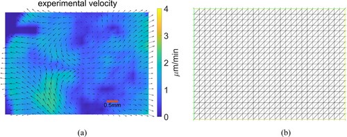We also note that the initial velocity ${\mathbf{u}}^0$ and the initial stress ${\mathbf{f}}^0$ is still zero everywhere in the Algorithm that follows. Figure 2(a) shows the measured velocity field of a chick embryo at stage HH2 of gastrulation, when the streak starts to form. Figure 2(b) shows the corresponding mesh with 1120 identical triangles for using the finite element method.

Figure 2. Velocity data and the mesh. (a) Experimental velocity field at stage HH2 of development. Velocity vectors are shown on a $28\times 20$ grid. The red scale bar is 0.5 millimeter in length. (b) Finite element mesh based on the velocity data.

To compute the numerical force distributions, we apply Algorithm ?? to the data for every time point. Specifically, we use the finite element method to compute the state scheme (34(34) $\{\begin{array}{ll}{\displaystyle (\frac{{\mathbf{U}}^k-{\mathbf{U}}^{k-1}}{\mathrm{\Delta }t},\tilde{\mathbf{u}})+a_{St}({\mathbf{U}}^k,\tilde{\mathbf{u}})+b_{St}(P^k,\tilde{\mathbf{u}})=({\mathbf{f}}^k,\tilde{\mathbf{u}}),}& \mathrm{\forall }\tilde{\mathbf{u}}\in U_h,\\ {\displaystyle b_{St}(\tilde{p},{\mathbf{U}}^k)-\epsilon (P^k,\tilde{p})=0,}& \mathrm{\forall }\tilde{p}\in W_h,\\ {\mathbf{U}}^0=0.\end{array}$(34) ) and the adjoint scheme (35(35) $\{\begin{array}{ll}{\displaystyle (\frac{{\mathbf{V}}^{k-1}-{\mathbf{V}}^k}{\mathrm{\Delta }t},\tilde{\mathbf{v}})+a_{Ad}({\mathbf{V}}^{k-1},\tilde{\mathbf{v}})-b_{Ad}(Q^{k-1},\tilde{\mathbf{v}})=({\mathbf{U}}^k-{\overline{\mathbf{u}}}^k,\tilde{\mathbf{v}}),}& \mathrm{\forall }\tilde{\mathbf{v}}\in U_h,\\ {\displaystyle b_{Ad}(\tilde{q},{\mathbf{V}}^{k-1})-\epsilon (Q^{k-1},\tilde{q})=0,}& \mathrm{\forall }\tilde{q}\in W_h,\\ {\mathbf{V}}^N=0.\end{array}$(35) ), and the conjugate gradient method to derive the optimal stress $\mathbf{f}$ on the domain.

First, we presents Figures 3 and 4 below to compare the numerical velocity fields $\mathbf{u}$ with the experimental velocity fields $\overline{\mathbf{u}}$ and the corresponding numerical stress distributions acting on chick embryo at 4 successive time intervals taken 30 min apart. From these figures, we can see that the experimentally measured velocity fields can be consistently matched by the numerical velocity fields, as shown by the small error between the numerical and experimental velocity (Table 1).

Figure 3. Comparing results. The red scale bar is 0.5 millimeter in length. (c) Experimental velocity at time $t_I$. (d) Experimental velocity at time $t_{II}$. (e) Numerical velocity at time $t_I$. (f) Numerical velocity at time $t_{II}$. (g) Numerical stress at time $t_I$. (h) Numerical stress at time $t_{II}$.

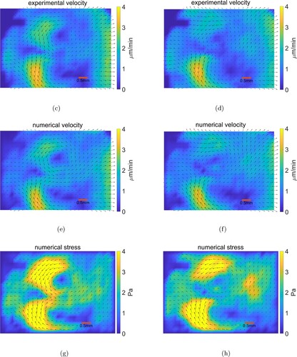
Figure 4. Comparing results. The red scale bar is 0.5 millimeter in length. (i) Experimental velocity at time $t_{III}$. (j) Experimental velocity at time $t_{IV}$ (k) Numerical velocity at time $t_{III}$ (l) Numerical velocity at time $t_{IV}$. (m) Numerical stress at time $t_{III}$ (n) Numerical stress at time $t_{IV}$.

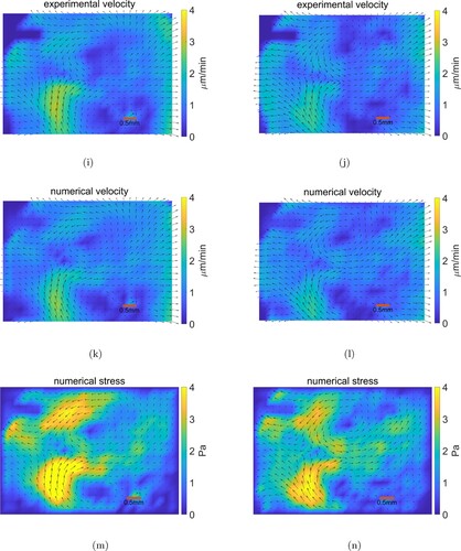
Table 1. The relative velocity error regarding to different time intervals.

Time interval	$t_I$	$t_{II}$	$t_{III}$	$t_{IV}$
Relative velocity error	$11.25\mathrm{\%}$	$9.30\mathrm{\%}$	$11.69\mathrm{\%}$	$11.89\mathrm{\%}$

(36) $Relativevelocityerror=\frac{\Vert {\mathbf{U}}^N-{\overline{\mathbf{u}}}^N{\Vert }_{0,\mathrm{\Omega }}^2}{\Vert {\overline{\mathbf{u}}}^N{\Vert }_{0,\mathrm{\Omega }}^2}$(36) Next, we consider the performance of Algorithm 1 with respect to the optimization of the iteration number. We determined the minimum value of objective functional for per unit area per hour as $J_{h,\mathrm{\Omega }}(\mathbf{U},\mathbf{f})$: (37) $J_{h,\mathrm{\Omega }}(\mathbf{U},\mathbf{f})=\frac{J(\mathbf{U},\mathbf{f})}{S_{\mathrm{\Omega }}T}=\frac{1}{S_{\mathrm{\Omega }}T}\sum _{k=1}^N\{\frac{1}{2}\Vert {\mathbf{U}}^k-{\overline{\mathbf{u}}}^k{\Vert }_{0,\mathrm{\Omega }}^2+\frac{\alpha }{2}\Vert {\mathbf{f}}^k{\Vert }_{0,\mathrm{\Omega }}^2\}\mathrm{\Delta }t,$(37) where $S_{\mathrm{\Omega }}$ is the area value of the domain. Figure 5 depicts the minimum value of the objective functional $J_{h,\mathrm{\Omega }}(\mathbf{U},\mathbf{f})$ along the optimization process at the four successive time intervals $(t_I,t_{II},t_{III},t_{IV})$. For these four time points, the numerical experiments showed that Algorithm 1 takes less than 50 optimization iterations to converge to the required accuracy. The minimum value of $J_{h,\mathrm{\Omega }}(\mathbf{U},\mathbf{f})$ decreases sharply at the beginning of optimization iterations, followed by an increasingly smooth decrease during further iterations until it reaches a minimum.

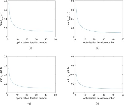
Figure 5. Minimum value of $J_{h,\mathrm{\Omega }}(\mathbf{U},\mathbf{f})$ during the optimization process. (o) at $t_I$ (p) at $t_{II}$ (q) at $t_{III}$ (r) at $t_{IV}$.

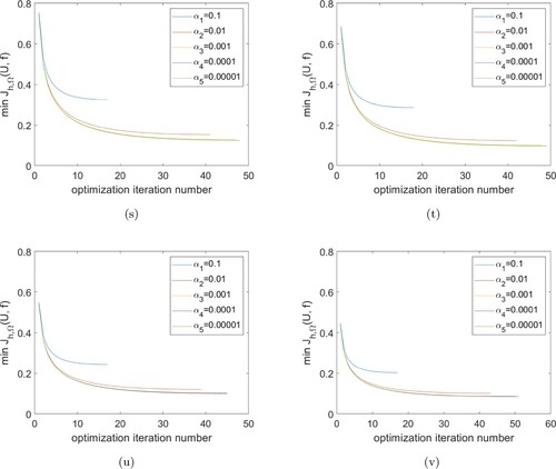
Finally, we discuss the influence of different choices α on the convergence of Algorithm 1. Table 2 shows the results of the optimization of the iteration number with different α used at the four successive time intervals.

Table 2. Relationship between α and optimization iteration number.

	Optimization iteration number
Time intervals	${\alpha }_1=0.1$	${\alpha }_2=0.01$	${\alpha }_3=0.001$	${\alpha }_4=0.0001$	${\alpha }_5=0.00001$
$t_I$	17	41	47	48	48
$t_{II}$	18	42	48	49	49
$t_{III}$	17	39	45	45	46
$t_{IV}$	17	43	50	51	51

Table 2 shows that the iteration number increases with the decreasing of α. Although α decreases by orders of magnitude from the initial choice of $\alpha =0.1$, the optimization iteration numbers remain almost unchanged. This means that a smaller choice of α does not accelerate the convergence of Algorithm 1 greatly. Figure 6 shows the minimum value $min{J}_{h,\mathrm{\Omega }}(\mathbf{U},\mathbf{f})$ for the optimization process at different α values. In each cases these values decrease sharply at the beginning of optimization iterations, followed by a much slower decrease to the end of iterations.

Figure 6. Minimum value of $J_{h,\mathrm{\Omega }}(\mathbf{U},\mathbf{f})$ during the optimization process for different values of α. (s) at $t_I$ (t) at $t_{II}$ (u) at $t_{III}$ (v) at $t_{IV}$.

5. Conclusions

In this paper, we have presented an inverse problem and a numerical method for a Stokes flow control model for a real biological problem, that is deriving stress distributions from tissue velocity fields measured during the early stages of chick embryo gastrulation. The inverse problem has been described through an optimal control model to determine the unknown stress distributions $\mathbf{f}$ that drive the tissue flows. We utilized the Lagrange multiplier method to derive the optimality system with the state equations, the adjoint equations and the optimality conditions. A finite element method was used to discretize these equations. The conjugate gradient method was formulated and applied as the optimization algorithm for the solution of the optimal control problem. We performed some numerical experiments and compared the computed results with the experiment data. These experiments indicated that the experimental data of the velocity fields can be closely matched by the computed data. It is interesting to note that although the experimental velocity data are not completely divergence-free, the proposed procedure is sufficiently robust to generate the velocity fields that are very close to those observed experimentally. The proposed method allows for the first time to generate plausible stress distributions that control tissue flow during chick gastrulation. Due to the very high viscosity of the tissue, making it a severely overdamped system, it is to be expected that the active stress distributions generated in the tissue closely match the observed velocity profiles, which appears indeed to be the case. The here proposed inverse Stokes problem and the solution using control theorey should have wide applicability to estimate tissue stresses driving important morphogenetic events during embryonic development such as gastrulation.

Disclosure statement

No potential conflict of interest was reported by the author(s).

Additional information

Funding

This work was supported by BBSRC [grant number BB/N009789/1] for the experimental work and China Scholarship Council [grant number 201506130077].

References

- P. Chandrashekar, S. Roy, and A.S.V. Murthy, A variational approach to estimate incompressible fluid flows, Proc. Math. Sci. 127 (2017), pp. 175–201.
- M. Chuai, D. Hughes, and C.J. Weijer, Collective epithelial and mesenchymal cell migration during gastrulation, Curr. Genomics. 13 (2012), pp. 267–277.
- M. Chuai and C.J. Weijer, The mechanisms underlying primitive streak formation in the chick embryo, Curr. Top. Dev. Biol. 81 (2008), pp. 135–156.
- M. Chuai and C.J. Weijer, Regulation of cell migration during chick gastrulation, Curr. Opin. Gen. Dev. 19(4) (2009), pp. 343–349.
- M. Chuai, W. Zeng, X. Yang, V. Boychenko, J.A. Glazier, and C.J. Weijer, Cell movement during chick primitive streak formation, Dev. Biol. 296(1) (2006), pp. 137–149.
- R. Courant, Variational methods for the solution of problems of equilibrium and vibrations, Bull. Am. Math. Soc. 49(1) (1943), pp. 1–23.
- F. Hecht, New development in freefem++, J Numer. Math. 20(3-4) (2012), pp. 251–265.
- J.C. Heinrich and C.A. Vionnet, The penalty method for the Navier–Stokes equations, Arch. Comput. Methods Eng. 2(2) (1995), pp. 51–65.
- B. Horn and B. Schunck, Determining optical flow, Artif. Intell. 17 (1981), pp. 185–203.
- A. Kirsch, An Introduction to the Mathematical Theory of Inverse Problems, Springer-Verlag, Berlin, Heidelberg, 1996.
- L. Lasdon, S. Mitter, and A. Waren, The conjugate gradient method for optimal control problems, IEEE. Trans. Automat. Contr. 12(2) (1967), pp. 132–138.
- P. Lin, A sequential regularization methods for time-dependent incompressibel Navier–Stokes equations, SIAM. J. Numer. Anal. 34(3) (1997), pp. 1051–1071.
- J.L. Lions, Optimal Control of Systems Governed by Partial Differential Equations, Springer-Verlag, Berlin, 1971.
- X.L. Lu and P. Lin, Error estimate of the P1 nonconforming finite element method for the penalized unsteady Navier–Stokes equations, Numer. Math. 115(2) (2010), pp. 261–287.
- H.M. Park and O.Y. Chung, On the solution of an inverse natural convection problem using various conjugate gradient methods, Int. J. Numer. Methods. Eng. 47 (2000), pp. 821–842.
- E. Polak, An historical survey of computational methods in optimal control, SIAM Rev. 15(2) (1973), pp. 553–584.
- A. Rösch and B. Vexler, Optimal control of the stokes equations: A priori error analysis for finite element discretization with postprocessing, SIAM. J. Numer. Anal. 44 (2006), pp. 1903–1920.
- S. Roy, M. Annunziato, and A. Borzì, A Fokker–Planck feedback control-constrained approach for modelling crowd motion, J. Comput. Theor. Transp. 45(6) (2016), pp. 442–458.
- S. Roy, M. Annunziato, A. Borzì, and C Klingenberg, A Fokker–Planck approach to control collective motion, Comput. Optim. Appl. 69 (2018), pp. 423–459.
- S. Roy, P. Chandrashekar, and A.S.V. Murthy, A variational approach to optical flow estimation of unsteady incompressible flows, Int. J. Adv. Eng. Sci. Appl. Math. 7 (2015), pp. 149–167.
- E. Rozbicki, M. Chuai, A. Karjalainen, F. Song, H. Sang, R. Martin, H.-J. Knölker, M. Macdonald, and C.J. Weijer, Myosin-II-mediated cell shape changes and cell intercalation contribute to primitive streak formation, Nat. Cell. Biol. 17 (2015), pp. 397–408.
- P. Ruhnau and C. Schnorr, Optical stokes flow estimation: An imaging-based control approach, Exp. Fluids. 42 (2007), pp. 61–78.
- S.A. Sandersius, M. Chuai, C.J. Weijer, and T.J. Newman, A ‘chemotactic dipole’ mechanism for large-scale vortex motion during primitive streak formation in the chick embryo, Phys. Biol. 8(4) (2011), pp. 045008.
- J. Shen, On error estimates of the penalty method for unsteady Navier–Stokes equations, SIAM. J. Numer. Anal. 32(2) (1995), pp. 386–403.
- R. Shewchuk J, An Introduction to the Conjugate Gradient Method Without the Agonizing Pain, Carnegie Mellon University, USA, 1994.
- C.D. Stern Gastrulation: From Cells to Embryo, Cold Spring Harbor Laboratory Press, New York, 2004. 219–232.
- D. Sweetman, L. Wagstaff, O. Cooper, C.J. Weijer, and A. Munsterberg, The migration of paraxial and lateral plate mesoderm cells emerging from the late primitive streak is controlled by different wnt signals, BMC. Dev. Biol. 8 (2008), pp. 63–78.
- R. Temam, Une méthode d'approximation des solutions des équations de Navier–Stokes, Bull. Sci. Math. 98 (1968), pp. 115–152.
- W. Thielicke and E.J. Stamhuis, Pivlab – towards user-friendly affordable and accurate digital particle image velocimetry in matlab, J. Open Res. Softw. 2(1) (2014), pp. e30.
- F. Troltzsch, Optimal Control of Partial Differential Equations: Theory, Methods and Applications, American mathematical society, USA, 2010.
- L. Vakaet, Cinephotomicrographic investigations of gastrulation in the chick blastoderm, Arch. Biol. (Liege) 81 (1970), pp. 387–426.
- B. Vasiev, A. Balter, M. Chaplain, J.A. Glazier, and C.J. Weijer, Modeling gastrulation in the chick embryo: Formation of the primitive streak, PLoS. ONE. 5(5) (2010), pp. e10571.
- X. Yang, H. Chrisman, and C.J. Weijer, PDGF signalling controls the migration of mesoderm cells during chick gastrulation by regulating N-cadherin expression, Development 135(21) (2008), pp. 3521–3530.