Optimality conditions for a class of E-differentiable vector optimization problems with interval-valued objective functions under E-invexity

Abstract

In this paper, a class of E-differentiable multiobjective programming with multiple objective functions and with both inequality and equality constraints is considered. The so-called E-Karush–Kuhn–Tucker necessary optimality conditions for a (weak LS-Pareto) LS-Pareto solution are established for the considered E-differentiable vector optimization problem with the multiple interval-valued objective functions. Also several sufficient optimality conditions for both LU and LS order relations are derived for such interval-valued vector optimization problems under (generalized) E-invexity hypotheses.

Keywords:

• E-differentiable interval-valued objective function
• E-differentiable function
• E-Karush–Kuhn–Tucker optimality conditions
• LU and LS-E-invex functions

AMS Classification::

• 90C29
• 90C30
• 90C46
• 90C26

1. Introduction

In mathematical programming, the coefficients of problems are assumed to be fixed in value. However, there are many situations where this assumption is not valid because of unconfirmed environments. In such cases, the decision-making methods which solve extremum problems with uncertainty are needed. The interval analysis provides strict enclosures of the solution to a mathematical model. In this way, we can at least know for sure what a mathematical model tells us, and, from that, we might determine whether it properly represent reality. Optimization problems using inexact data are strongly connected to interval-valued optimization problems. In recent years, interval-valued optimization problems have been studied by many researchers in several directions (see, e.g., [6,7,9–11,13–20,24–28,31], and others).

Wu [30–33] derived the KKT conditions for optimization problems with interval-valued objective functions. Sun and Wang [29] gave the concept of an LU-optimal solution to nondifferentiable optimization problems with the interval-valued objective function and constraint crisp functions. Zhang et al. [35] extended the concepts of invexity and preinvexity to interval-valued functions and established the KKT conditions for a class of optimization problems with an interval-valued objective function. Jayswal et al. [12] established sufficient conditions for KKT optimality conditions for a feasible solution to be an LU-optimal solution under invexity hypotheses.

Youness [34] introduced the concepts of E-convex sets and E-convex functions. Megahed et al. [23] presented the concept of an E-differentiable function which transforms a (not necessarily) differentiable function to a differentiable function based on the effect of an operator $E:R^n\to R^n$. Antczak and Abdulaleem [4] established the so-called E-optimality conditions for the E-differentiable E-convex vector optimization problem with the multiple interval-valued objective functions with both inequality and equality constraints. Abdulaleem [3] extended the aforesaid results for a new class of not necessarily differentiable multicriteria optimization problems, namely for E-differentiable multiobjective programming problems involving E-type I functions.

In this paper, the class of E-differentiable E-invex multiobjective programming problem with the multiple interval-valued objective functions and with both inequality and equality constraints is considered. Based on the LU and LS order relations, we define various concepts of Pareto optimality for the considered interval-valued multiobjective programming problems. For this interval-valued multiobjective programming problem, we derive Karush–Kuhn–Tucker necessary optimality conditions for a weak LS-E-Pareto solution for the considered E-differentiable vector optimization problem with the multiple interval-valued objective functions. Further, we establish several sufficient optimality conditions of Karush–Kuhn–Tucker type for a class of E-differentiable interval-valued programming problems with (generalized) E-invexity functions.

2. Preliminaries

Let $R^n$ be the n-dimensional Euclidean space and $R_{+}^n$ be its nonnegative orthant. The following convention for equalities and inequalities will be used in the paper.

For any vectors $x=(x_1,x_2,\dots ,x_n{)}^T$ and $y=(y_1,y_2,\dots ,y_n{)}^T$ in $R^n$, we define:

1. x = y if and only if $x_i=y_i$ for all $i=1,2,\dots ,n$;

2. x>y if and only if $x_i>y_i$ for all $i=1,2,\dots ,n$;

3. $x\geqq y$ if and only if $x_i\geqq y_i$ for all $i=1,2,\dots ,n$;

4. $x\ge y$ if and only if $x\geqq y$ and $x\ne y$.

We denote by ${\mathcal{K}}_C$, the family of all bounded closed intervals in $R$, i.e. ${\mathcal{K}}_C=\{[a,b];a,b\in R\mathrm{and}a⩽b\},$where the width of the interval is b−a.

If $A\in {\mathcal{K}}_C$, then we adopt the notation $A=[a^L,a^U]$, where $a^L$ and $a^U$ mean the lower and upper bounds of A, respectively. In other words, if $A=[a^L,a^U]\in {\mathcal{K}}_C$, then $A=[a^L,a^U]=\{x\in R:a^L\leqq x\leqq a^U\}$. If $a^L=a^U=a$, then $A=[a,a]=a$ is a real number.

Let $A=[a^L,a^U]$, $B=[b^L,b^U]\in {\mathcal{K}}_C$. Then, by definition, we have (1) $\begin{array}{rl}A+B& =[a^L,a^U]+[b^L,b^U]=[a^L+b^L,a^U+b^U],\end{array}$(1) (2) $\begin{array}{rl}k\cdot A& =k[a^L,a^U]=\begin{array}{ccc}[k{a}^L,k{a}^U]& \mathrm{if}& k\geqq 0,\\ [k{a}^U,k{a}^L]& \mathrm{if}& k<0.\end{array}\end{array}$(2) From (1(1) $\begin{array}{rl}A+B& =[a^L,a^U]+[b^L,b^U]=[a^L+b^L,a^U+b^U],\end{array}$(1) ) and (2(2) $\begin{array}{rl}k\cdot A& =k[a^L,a^U]=\begin{array}{ccc}[k{a}^L,k{a}^U]& \mathrm{if}& k\geqq 0,\\ [k{a}^U,k{a}^L]& \mathrm{if}& k<0.\end{array}\end{array}$(2) ), we have $-A=-[a^L,a^U]=[-a^U,-a^L]$ and $B-A=B+(-A)=[b^L-a^U,b^U-a^L]$.

In interval mathematics, an order relation is often used to rank interval numbers and it implies that an interval number is better than another but not that one is larger than another.

Definition 2.1

Let $A=[a^L,a^U]$ and $B=[b^L,b^U]$ be two sets in ${\mathcal{K}}_C$.

1. $A{\leqq }_{LU}B$ if and only if $a^L\leqq b^L$ and $a^U\leqq b^U$.

2. $A{<}_{LU}B$ if and only if $A{\leqq }_{LU}B$ and $A\ne B$. Equivalently, $A{<}_{LU}B$ if and only if (3) $\{\begin{array}{l}{a}^L<b^L\\ a^U\leqq b^U\end{array}\mathrm{or}\{\begin{array}{l}{a}^L\leqq b^L\\ a^U<b^U\end{array}\mathrm{or}\{\begin{array}{l}{a}^L<b^L\\ a^U<b^U\end{array}.$(3)

For $A=[a^L,a^U]$, the width (spread) of A is defined by $w(A)=a^S=a^U-a^L$. We propose the order relation between A and B by considering the maximization and minimization problems separately:

1. For maximization, we write $A{\geqq }_{LS}B$ if and only if $a^U\geqq b^U$ and $a^S\leqq b^S$.

2. For minimization, we write $A{\leqq }_{LS}B$ if and only if $a^L\leqq b^L$ and $a^S\leqq b^S$.

In this paper, we consider only the minimization problem. In this sense, we also write $A{<}_{LS}B$ if and only if $A{\leqq }_{LS}B$ and $A\ne B$. Equivalently, $A{<}_{LS}B$ if and only if (4) $\{\begin{array}{l}{a}^L<b^L\\ a^S\leqq b^S\end{array}\mathrm{or}\{\begin{array}{l}{a}^L\leqq b^L\\ a^S<b^S\end{array}\mathrm{or}\{\begin{array}{l}{a}^L<b^L\\ a^S<b^S\end{array}.$(4)

Proposition 2.2

Let A and B be two sets in ${\mathcal{K}}_C$. If $A{\leqq }_{LS}B$, then $A{\leqq }_{LU}B$.

Proof.

Since A and B are two sets in ${\mathcal{K}}_C$ such that $A{\leqq }_{LS}B$, then $a^L\leqq b^L$ and $a^S\leqq b^S$, that is, $a^L\leqq b^L$ and $a^U-a^L\leqq b^U-b^L$. Thus $a^U\leqq b^U$. Therefore, $A{\leqq }_{LU}B$.

It should be noted that the converse of Proposition 2.2 is not true. For example, if we consider $A=[-2,0]$ and $B=[-1,0]$, then $A{\leqq }_{LU}B$, but $A{\nleqq }_{LS}B$.

Now, we give the definition of an E-invex set introduced by Abdulaleem [1].

Definition 2.3

A set $M\subseteq R^n$ is said to be E-invex with respect to an operator $E:R^n\to R^n$ if and only if there exists a vector-valued function $\eta :R^n\times R^n\to R^n$ such that the relation $E\left(x^{\ast }\right)+\lambda \eta (E\left(x\right),E\left(x^{\ast }\right))\in M$holds for all $x,x^{\ast }\in M$ and $\lambda \in [0,1]$.

Definition 2.4

Let M be an open set in $R^n$. A function $f:M\to {\mathcal{K}}_C$ is called an interval-valued function if $f(x)=[f^L(x),f^S(x)]$ with $f^L(x),f^S(x):M\to R$ such that $f^L(x)\leqq f^S(x)$ for each $x\in M$.

Definition 2.5

Let M be an open set in $R^n$. An interval-valued function $f:M\to {\mathcal{K}}_C$ with $f(x)=[f^L(x),f^U(x)]$ is called weakly differentiable at x if the real-valued functions $f^L$ and $f^U$ are differentiable at x (in the usual sense).

Now, we give the definition of E-differentiability to the case of an interval-valued function given by Antczak and Abdulaleem [5].

Definition 2.6

Let $E:R^n\to R^n$, $f:R^n\to {\mathcal{K}}_C$ and $x^{\ast }\in R^n$. It is said that f is weakly E-differentiable at $x^{\ast }$ if and only if $f^L\circ E$ and $f^U\circ E$ are differentiable at $x^{\ast }$ (in the usual sense), that is, (5) $\begin{array}{rl}& (f^L\circ E)\left(x\right)=(f^L\circ E)\left(x^{\ast }\right)+\mathrm{\nabla }(f^L\circ E)\left(x^{\ast }\right)(x-x^{\ast })+{\theta }^L(x^{\ast },x-x^{\ast })\Vert x-x^{\ast }\Vert ,\end{array}$(5) (6) $\begin{array}{rl}& (f^U\circ E)\left(x\right)=(f^U\circ E)\left(x^{\ast }\right)+\mathrm{\nabla }(f^U\circ E)\left(x^{\ast }\right)(x-x^{\ast })+{\theta }^U(x^{\ast },x-x^{\ast })\Vert x-x^{\ast }\Vert \end{array}$(6) where ${\theta }^L(x^{\ast },x-x^{\ast })\to 0$, ${\theta }^U(x^{\ast },x-x^{\ast })\to 0$ as $x\to x^{\ast }$.

Definition 2.7

Let $E:R^n\to R^n$, $f:R^n\to {\mathcal{K}}_C$ and $x^{\ast }\in R^n$. It is said that f is weakly E-differentiable at $x^{\ast }$ if and only if $f^L\circ E$ and $f^S\circ E$ are differentiable at $x^{\ast }$ (in the usual sense), that is, (7) $\begin{array}{rl}& (f^L\circ E)\left(x\right)=(f^L\circ E)\left(x^{\ast }\right)+\mathrm{\nabla }(f^L\circ E)\left(x^{\ast }\right)(x-x^{\ast })+{\theta }^L(x^{\ast },x-x^{\ast })\Vert x-x^{\ast }\Vert ,\end{array}$(7) (8) $\begin{array}{rl}& (f^S\circ E)\left(x\right)=(f^S\circ E)\left(x^{\ast }\right)+\mathrm{\nabla }(f^S\circ E)\left(x^{\ast }\right)(x-x^{\ast })+{\theta }^S(x^{\ast },x-x^{\ast })\Vert x-x^{\ast }\Vert \end{array}$(8) where ${\theta }^L(x^{\ast },x-x^{\ast })\to 0$, ${\theta }^S(x^{\ast },x-x^{\ast })\to 0$ as $x\to x^{\ast }$.

The definition of an E-differentiable E-invex function was introduced by Abdulaleem [1]. Now, for convenience, we recall this definition.

Definition 2.8

Let $E:R^n\to R^n$ and $f:R^n\to R$ be E-differentiable at $x^{\ast }$. If there exists a vector-valued function $\eta :R^n\times R^n\to R^n$ such that the inequality (9) $f(E(x))-f(E(x^{\ast }))\geqq \mathrm{\nabla }f(E(x^{\ast }))\eta (E(x),E(x^{\ast }))$(9) holds for all $x\in R^n$, then f is said to be an E-differentiable E-invex function at $x^{\ast }$ on $R^n$ with respect to η. If (9(9) $f(E(x))-f(E(x^{\ast }))\geqq \mathrm{\nabla }f(E(x^{\ast }))\eta (E(x),E(x^{\ast }))$(9) ) is fulfilled for all $x^{\ast }\in R^n$, then f is said to be an E-differentiable E-invex function on $R^n$ with respect to η. If (9(9) $f(E(x))-f(E(x^{\ast }))\geqq \mathrm{\nabla }f(E(x^{\ast }))\eta (E(x),E(x^{\ast }))$(9) ) is fulfilled for all $x,x^{\ast }\in M\subset R^n$, where M is an E-invex set with respect to η, then f is said to be an E-differentiable E-invex function on M with respect to η.

Now, we extend the definition of an E-invex function to the case of weakly E-differentiable interval-valued functions.

Definition 2.9

Let $E:R^n\to R^n$ and $f:R^n\to {\mathcal{K}}_C$ be a weakly E-differentiable interval-valued function at $x^{\ast }$. If there exists a vector-valued function $\eta :R^n\times R^n\to R^n$ such that the inequalities (10) $\begin{array}{rl}& f^L(E(x))-f^L(E(x^{\ast }))\geqq \mathrm{\nabla }{f}^L(E(x^{\ast }))\eta (E(x),E(x^{\ast })),\end{array}$(10) (11) $\begin{array}{rl}& f^U(E(x))-f^U(E(x^{\ast }))\geqq \mathrm{\nabla }{f}^U(E(x^{\ast }))\eta (E(x),E(x^{\ast }))\end{array}$(11) hold for all $x\in R^n$, then f is said to be LU-E-invex at $x^{\ast }$ on $R^n$ with respect to η. If (10(10) $\begin{array}{rl}& f^L(E(x))-f^L(E(x^{\ast }))\geqq \mathrm{\nabla }{f}^L(E(x^{\ast }))\eta (E(x),E(x^{\ast })),\end{array}$(10) ) and (11(11) $\begin{array}{rl}& f^U(E(x))-f^U(E(x^{\ast }))\geqq \mathrm{\nabla }{f}^U(E(x^{\ast }))\eta (E(x),E(x^{\ast }))\end{array}$(11) ) are fulfilled for all $x^{\ast }\in R^n$, then f is said to be LU-E-invex on $R^n$ with respect to η. If (10(10) $\begin{array}{rl}& f^L(E(x))-f^L(E(x^{\ast }))\geqq \mathrm{\nabla }{f}^L(E(x^{\ast }))\eta (E(x),E(x^{\ast })),\end{array}$(10) ) and (11(11) $\begin{array}{rl}& f^U(E(x))-f^U(E(x^{\ast }))\geqq \mathrm{\nabla }{f}^U(E(x^{\ast }))\eta (E(x),E(x^{\ast }))\end{array}$(11) ) are fulfilled for all $x,x^{\ast }\in M\subset R^n$, then f is said to be LU-E-invex on M with respect to η.

Definition 2.10

Let $E:R^n\to R^n$ and $f:R^n\to {\mathcal{K}}_C$ be a weakly E-differentiable interval-valued function at $x^{\ast }$. If there exists a vector-valued function $\eta :R^n\times R^n\to R^n$ such that the inequalities (12) $\begin{array}{rl}& f^L(E(x))-f^L(E(x^{\ast }))\geqq \mathrm{\nabla }{f}^L(E(x^{\ast }))\eta (E(x),E(x^{\ast })),\end{array}$(12) (13) $\begin{array}{rl}& f^S(E(x))-f^S(E(x^{\ast }))\geqq \mathrm{\nabla }{f}^S(E(x^{\ast }))\eta (E(x),E(x^{\ast }))\end{array}$(13) hold for all $x\in R^n$, then f is said to be LS-E-invex at $x^{\ast }$ on $R^n$ with respect to η. If (12(12) $\begin{array}{rl}& f^L(E(x))-f^L(E(x^{\ast }))\geqq \mathrm{\nabla }{f}^L(E(x^{\ast }))\eta (E(x),E(x^{\ast })),\end{array}$(12) ) and (13(13) $\begin{array}{rl}& f^S(E(x))-f^S(E(x^{\ast }))\geqq \mathrm{\nabla }{f}^S(E(x^{\ast }))\eta (E(x),E(x^{\ast }))\end{array}$(13) ) are fulfilled for all $x^{\ast }\in R^n$, then f is said to be LS-E-invex on $R^n$ with respect to η. If (12(12) $\begin{array}{rl}& f^L(E(x))-f^L(E(x^{\ast }))\geqq \mathrm{\nabla }{f}^L(E(x^{\ast }))\eta (E(x),E(x^{\ast })),\end{array}$(12) ) and (13(13) $\begin{array}{rl}& f^S(E(x))-f^S(E(x^{\ast }))\geqq \mathrm{\nabla }{f}^S(E(x^{\ast }))\eta (E(x),E(x^{\ast }))\end{array}$(13) ) are fulfilled for all $x,x^{\ast }\in M\subset R^n$, then f is said to be LS-E-invex on M with respect to η.

Proposition 2.11

Let $E:R^n\to R^n$ and $f:R^n\to {\mathcal{K}}_C$ be a weakly E-differentiable interval-valued function at $x^{\ast }$. Then we have following properties:

(i)	f is LU-E-invex at $x^{\ast }$ if and only if $f^L$ and $f^U$ are E-invex E-differentiable functions at $x^{\ast }$.
(ii)	f is LS-E-invex at $x^{\ast }$ if and only if $f^L$ and $f^S$ are E-invex E-differentiable functions at $x^{\ast }$.
(iii)	If f is LS-E-invex at $x^{\ast }$, then f is LU-E-invex at $x^{\ast }$.

Proof.

The proof of (i), (ii) follows directly from Definitions 2.9 and 2.10 and (iii) follows directly from Proposition 2.2.

Now, we give an example of such an LU-E-invex function which is not LS-E-invex.

Example 2.12

Let $E:R\to R$, $f:[0,\mathrm{\infty })\to {\mathcal{K}}_C$ be a weakly E-differentiable interval-valued function on $[0,\mathrm{\infty })$ defined by $f(x)=-[1,2]\sqrt[3]{x},E(x)=x^3,\eta (E(x),E(x^{\ast }))=\{\begin{array}{ll}x-x^{\ast }& \text{if}x\geqq x^{\ast },\\ 0& \text{if}x<x^{\ast }.\end{array}$From above we have $f^L(x)=-2\sqrt[3]{x}$ and $f^U(x)=-\sqrt[3]{x}$, therefore $f^S(x)=\sqrt[3]{x}$. Then, by Definition 2.9, f is LU-E-invex on $[0,\mathrm{\infty })$ with respect to η given above, while f is not LS-E-invex on $[0,\mathrm{\infty })$ with respect to η given above, because for x = 1 and $x^{\ast }=2$, we have $f^S(E(x))-f^S(E(x^{\ast }))=-1\ngeqq 0=\mathrm{\nabla }{f}^S(E(x^{\ast }))\eta (E(x),E(x^{\ast })).$Hence, by Definition 2.10, f is not LS-E-invex on $[0,\mathrm{\infty })$ with respect to η given above (see Figure 1).

Figure 1. Graphical view of $f(E(x))$ in Example 2.12.

Definition 2.13

Let $E:R^n\to R^n$ and $f:R^n\to {\mathcal{K}}_C$ be a weakly E-differentiable interval-valued function at $x^{\ast }$. If there exists a vector-valued function $\eta :R^n\times R^n\to R^n$ such that the inequalities (14) $\begin{array}{rl}& f^L(E(x))-f^L(E(x^{\ast }))>\mathrm{\nabla }{f}^L(E(x^{\ast }))\eta (E(x),E(x^{\ast })),\end{array}$(14) (15) $\begin{array}{rl}& f^U(E(x))-f^U(E(x^{\ast }))>\mathrm{\nabla }{f}^U(E(x^{\ast }))\eta (E(x),E(x^{\ast }))\end{array}$(15) hold for all $x\in R^n$ $(E(x)\ne E(x^{\ast }))$, then f is said to be strictly LU-E-invex at $x^{\ast }$ on $R^n$ with respect to η. If (14(14) $\begin{array}{rl}& f^L(E(x))-f^L(E(x^{\ast }))>\mathrm{\nabla }{f}^L(E(x^{\ast }))\eta (E(x),E(x^{\ast })),\end{array}$(14) ) and (15(15) $\begin{array}{rl}& f^U(E(x))-f^U(E(x^{\ast }))>\mathrm{\nabla }{f}^U(E(x^{\ast }))\eta (E(x),E(x^{\ast }))\end{array}$(15) ) are fulfilled for all $x^{\ast }\in R^n$, then f is said to be strictly LU-E-invex on $R^n$ with respect to η. If (14(14) $\begin{array}{rl}& f^L(E(x))-f^L(E(x^{\ast }))>\mathrm{\nabla }{f}^L(E(x^{\ast }))\eta (E(x),E(x^{\ast })),\end{array}$(14) ) and (15(15) $\begin{array}{rl}& f^U(E(x))-f^U(E(x^{\ast }))>\mathrm{\nabla }{f}^U(E(x^{\ast }))\eta (E(x),E(x^{\ast }))\end{array}$(15) ) are fulfilled for all $x,x^{\ast }\in M\subset R^n$ $(E(x)\ne E(x^{\ast }))$, then f is said to be strictly LU-E-invex on M with respect to η.

Definition 2.14

Let $E:R^n\to R^n$ and $f:R^n\to {\mathcal{K}}_C$ be a weakly E-differentiable interval-valued function at $x^{\ast }$. If there exists a vector-valued function $\eta :R^n\times R^n\to R^n$ such that the inequalities (16) $\begin{array}{rl}& f^L(E(x))-f^L(E(x^{\ast }))>\mathrm{\nabla }{f}^L(E(x^{\ast }))\eta (E(x),E(x^{\ast })),\end{array}$(16) (17) $\begin{array}{rl}& f^S(E(x))-f^S(E(x^{\ast }))>\mathrm{\nabla }{f}^S(E(x^{\ast }))\eta (E(x),E(x^{\ast }))\end{array}$(17) hold for all $x\in R^n$ $(E(x)\ne E(x^{\ast }))$, then f is said to be strictly LS-E-invex at $x^{\ast }$ on $R^n$ with respect to η. If (16(16) $\begin{array}{rl}& f^L(E(x))-f^L(E(x^{\ast }))>\mathrm{\nabla }{f}^L(E(x^{\ast }))\eta (E(x),E(x^{\ast })),\end{array}$(16) ) and (17(17) $\begin{array}{rl}& f^S(E(x))-f^S(E(x^{\ast }))>\mathrm{\nabla }{f}^S(E(x^{\ast }))\eta (E(x),E(x^{\ast }))\end{array}$(17) ) are fulfilled for all $x^{\ast }\in R^n(E(x)\ne E(x^{\ast }))$, then f is said to be strictly LS-E-invex on $R^n$ with respect to η. If (16(16) $\begin{array}{rl}& f^L(E(x))-f^L(E(x^{\ast }))>\mathrm{\nabla }{f}^L(E(x^{\ast }))\eta (E(x),E(x^{\ast })),\end{array}$(16) ) and (17(17) $\begin{array}{rl}& f^S(E(x))-f^S(E(x^{\ast }))>\mathrm{\nabla }{f}^S(E(x^{\ast }))\eta (E(x),E(x^{\ast }))\end{array}$(17) ) are fulfilled for all $x,x^{\ast }\in M\subset R^n(E(x)\ne E(x^{\ast }))$, then f is said to be strictly LS-E-invex on M with respect to η.

Now, we prove a sufficient condition for an E-differentiable interval-valued function to be E-invex.

Theorem 2.15

Let $E:R^n\to R^n$ and $f:R^n\to {\mathcal{K}}_C$ be a weakly E-differentiable interval-valued function at $x^{\ast }$ with respect to the vector-valued function $\eta :R^n\times R^n\to R^n$ such that the inequalities (18) $\begin{array}{rl}& f^L(E\left(x^{\ast }\right)+\lambda \eta (E\left(x\right),E\left(x^{\ast }\right))\leqq \lambda f^L\left(E\left(x\right)\right)+(1-\lambda )f^L\left(E\left(x^{\ast }\right)\right),\end{array}$(18) (19) $\begin{array}{rl}& f^U(E\left(x^{\ast }\right)+\lambda \eta (E\left(x\right),E\left(x^{\ast }\right))\leqq \lambda f^U\left(E\left(x\right)\right)+(1-\lambda )f^U\left(E\left(x^{\ast }\right)\right)\end{array}$(19) hold for any $\lambda \in [0,1]$. Then, f is a weakly E-differentiable LU-E-invex interval-valued function with respect to η.

Proof.

By (18(18) $\begin{array}{rl}& f^L(E\left(x^{\ast }\right)+\lambda \eta (E\left(x\right),E\left(x^{\ast }\right))\leqq \lambda f^L\left(E\left(x\right)\right)+(1-\lambda )f^L\left(E\left(x^{\ast }\right)\right),\end{array}$(18) ) and (19(19) $\begin{array}{rl}& f^U(E\left(x^{\ast }\right)+\lambda \eta (E\left(x\right),E\left(x^{\ast }\right))\leqq \lambda f^U\left(E\left(x\right)\right)+(1-\lambda )f^U\left(E\left(x^{\ast }\right)\right)\end{array}$(19) ), we have that the inequalities (20) $\begin{array}{rl}& f^L(E\left(x^{\ast }\right)+\lambda \eta (E\left(x\right),E\left(x^{\ast }\right)))-f^L\left(E\left(x^{\ast }\right)\right)\leqq \lambda [f^L\left(E\left(x\right)\right)-f^L\left(E\left(x^{\ast }\right)\right)],\end{array}$(20) (21) $\begin{array}{rl}& f^U(E\left(x^{\ast }\right)+\lambda \eta (E\left(x\right),E\left(x^{\ast }\right)))-f^U\left(E\left(x^{\ast }\right)\right)\leqq \lambda [f^U\left(E\left(x\right)\right)-f^U\left(E\left(x^{\ast }\right)\right)]\end{array}$(21) hold for any $\lambda \in [0,1]$. Thus the above inequalities yields for any $\lambda \in [0,1]$, (22) $\begin{array}{rl}& \frac{f^L(E\left(x^{\ast }\right)+\lambda \eta (E\left(x\right),E\left(x^{\ast }\right)))-f^L\left(E\left(x^{\ast }\right)\right)}{\lambda }\leqq f^L\left(E\left(x\right)\right)-f^L\left(E\left(x^{\ast }\right)\right),\end{array}$(22) (23) $\begin{array}{rl}& \frac{f^U(E\left(x^{\ast }\right)+\lambda \eta (E\left(x\right),E\left(x^{\ast }\right)))-f^U\left(E\left(x^{\ast }\right)\right)}{\lambda }\leqq f^U\left(E\left(x\right)\right)-f^U\left(E\left(x^{\ast }\right)\right).\end{array}$(23) By assumption, f is weakly E-differentiable at $x^{\ast }$. Hence, by Definition 2.6, it follows that $f\circ E$ is differentiable at $x^{\ast }$. Therefore, letting $\lambda \to 0$, we obtain the inequalities (10(10) $\begin{array}{rl}& f^L(E(x))-f^L(E(x^{\ast }))\geqq \mathrm{\nabla }{f}^L(E(x^{\ast }))\eta (E(x),E(x^{\ast })),\end{array}$(10) ) and (11(11) $\begin{array}{rl}& f^U(E(x))-f^U(E(x^{\ast }))\geqq \mathrm{\nabla }{f}^U(E(x^{\ast }))\eta (E(x),E(x^{\ast }))\end{array}$(11) ).

Example 2.16

Let $E:R^2\to R^2$, $f:R^2\to {\mathcal{K}}_C$ be a weakly E-differentiable interval-valued function on $R^2$ defined by $f(x)=[\frac{1}{2},\frac{3}{2}](\sin \left(\sqrt[3]{x_1}\right)+\sin \left(\sqrt[3]{x_2}\right)-\sqrt[3]{64x_1}-\sqrt[3]{64x_2}),E(x_1,x_2)=(x_1^3,x_2^3).$Note that f is not an E-differentiable E-convex interval-valued function as can be seen by taking $x=-\pi$, $x^{\ast }=\pi$, since the inequalities (24) $\begin{array}{rl}& f^L\left(E\left(x\right)\right)-f^L\left(E\left(x^{\ast }\right)\right)<\mathrm{\nabla }{f}^L\left(E\left(x^{\ast }\right)\right)(E\left(x\right)-E\left(x^{\ast }\right)),\end{array}$(24) (25) $\begin{array}{rl}& f^U\left(E\left(x\right)\right)-f^U\left(E\left(x^{\ast }\right)\right)<\mathrm{\nabla }{f}^U\left(E\left(x^{\ast }\right)\right)(E\left(x\right)-E\left(x^{\ast }\right))\end{array}$(25) hold. Hence, by the definition of an E-differentiable E-convex interval-valued function introduced by Antczak and Abdulaleem [5], it follows that f is not an E-differentiable E-convex interval-valued function. However, the function f is an LU-E-invex function with respect to $\eta (E(x),E(x^{\ast }))=(\frac{\sin (x_1)-\sin (x_1^{\ast })-4x_1+4x_1^{\ast }}{\cos (x_1^{\ast })-4},\frac{\sin (x_2)-\sin (x_2^{\ast })-4x_2+4x_2^{\ast }}{\cos (x_2^{\ast })-4}).$

Now, we extend the concepts of generalized E-invexity introduced by Abdulaleem [1] for E-differentiable functions to the case of a weakly E-differentiable interval-valued function.

Definition 2.17

Let $E:R^n\to R^n$ and $f:R^n\to {\mathcal{K}}_C$ be a weakly E-differentiable interval-valued function at $x^{\ast }$. If there exists a vector-valued function $\eta :R^n\times R^n\to R^n$ such that the following relations (26) $\begin{array}{rl}& f^L(E(x))<f^L(E(x^{\ast }))\Rightarrow \mathrm{\nabla }{f}^L(E(x^{\ast }))\eta (E(x),E(x^{\ast }))<0,\end{array}$(26) (27) $\begin{array}{rl}& f^U(E(x))<f^U(E(x^{\ast }))\Rightarrow \mathrm{\nabla }{f}^U(E(x^{\ast }))\eta (E(x),E(x^{\ast }))<0\end{array}$(27) hold for all $x\in R^n$, then f is said to be pseudo LU-E-invex at $x^{\ast }$ on $R^n$ with respect to η. If (26(26) $\begin{array}{rl}& f^L(E(x))<f^L(E(x^{\ast }))\Rightarrow \mathrm{\nabla }{f}^L(E(x^{\ast }))\eta (E(x),E(x^{\ast }))<0,\end{array}$(26) ) and (27(27) $\begin{array}{rl}& f^U(E(x))<f^U(E(x^{\ast }))\Rightarrow \mathrm{\nabla }{f}^U(E(x^{\ast }))\eta (E(x),E(x^{\ast }))<0\end{array}$(27) ) are fulfilled for all $x^{\ast }\in R^n$, then f is said to be pseudo LU-E-invex on $R^n$ with respect to η. If (26(26) $\begin{array}{rl}& f^L(E(x))<f^L(E(x^{\ast }))\Rightarrow \mathrm{\nabla }{f}^L(E(x^{\ast }))\eta (E(x),E(x^{\ast }))<0,\end{array}$(26) ) and (27(27) $\begin{array}{rl}& f^U(E(x))<f^U(E(x^{\ast }))\Rightarrow \mathrm{\nabla }{f}^U(E(x^{\ast }))\eta (E(x),E(x^{\ast }))<0\end{array}$(27) ) are fulfilled for all $x,x^{\ast }\in M\subset R^n$, then f is said to be pseudo LU-E-invex on M with respect to η.

Definition 2.18

Let $E:R^n\to R^n$ and $f:R^n\to {\mathcal{K}}_C$ be a weakly E-differentiable interval-valued function at $x^{\ast }$. If there exists a vector-valued function $\eta :R^n\times R^n\to R^n$ such that the following relations: (28) $\begin{array}{rl}& f^L(E(x))<f^L(E(x^{\ast }))\Rightarrow \mathrm{\nabla }{f}^L(E(x^{\ast }))\eta (E(x),E(x^{\ast }))<0,\end{array}$(28) (29) $\begin{array}{rl}& f^S(E(x))<f^S(E(x^{\ast }))\Rightarrow \mathrm{\nabla }{f}^S(E(x^{\ast }))\eta (E(x),E(x^{\ast }))<0\end{array}$(29) hold for all $x\in R^n$, then f is said to be pseudo LS-E-invex at $x^{\ast }$ on $R^n$ with respect to η. If (28(28) $\begin{array}{rl}& f^L(E(x))<f^L(E(x^{\ast }))\Rightarrow \mathrm{\nabla }{f}^L(E(x^{\ast }))\eta (E(x),E(x^{\ast }))<0,\end{array}$(28) ) and (29(29) $\begin{array}{rl}& f^S(E(x))<f^S(E(x^{\ast }))\Rightarrow \mathrm{\nabla }{f}^S(E(x^{\ast }))\eta (E(x),E(x^{\ast }))<0\end{array}$(29) ) are fulfilled for all $x^{\ast }\in R^n$, then f is said to be pseudo LS-E-invex on $R^n$ with respect to η. If (28(28) $\begin{array}{rl}& f^L(E(x))<f^L(E(x^{\ast }))\Rightarrow \mathrm{\nabla }{f}^L(E(x^{\ast }))\eta (E(x),E(x^{\ast }))<0,\end{array}$(28) ) and (29(29) $\begin{array}{rl}& f^S(E(x))<f^S(E(x^{\ast }))\Rightarrow \mathrm{\nabla }{f}^S(E(x^{\ast }))\eta (E(x),E(x^{\ast }))<0\end{array}$(29) ) are fulfilled for all $x,x^{\ast }\in M\subset R^n$, then f is said to be pseudo LS-E-invex on M with respect to η.

Definition 2.19

Let $E:R^n\to R^n$ and $f:R^n\to {\mathcal{K}}_C$ be a weakly E-differentiable interval-valued function at $x^{\ast }$. If there exists a vector-valued function $\eta :R^n\times R^n\to R^n$ such that the following relations: (30) $\begin{array}{rl}& f^L(E(x))\leqq f^L(E(x^{\ast }))\Rightarrow \mathrm{\nabla }{f}^L(E(x^{\ast }))\eta (E(x),E(x^{\ast }))<0,\end{array}$(30) (31) $\begin{array}{rl}& f^U(E(x))\leqq f^U(E(x^{\ast }))\Rightarrow \mathrm{\nabla }{f}^U(E(x^{\ast }))\eta (E(x),E(x^{\ast }))<0\end{array}$(31) hold for all $x\in R^n$ $(E(x)\ne E(x^{\ast }))$, then f is said to be strictly pseudo LU-E-invex at $x^{\ast }$ on $R^n$ with respect to η. If (30(30) $\begin{array}{rl}& f^L(E(x))\leqq f^L(E(x^{\ast }))\Rightarrow \mathrm{\nabla }{f}^L(E(x^{\ast }))\eta (E(x),E(x^{\ast }))<0,\end{array}$(30) ) and (31(31) $\begin{array}{rl}& f^U(E(x))\leqq f^U(E(x^{\ast }))\Rightarrow \mathrm{\nabla }{f}^U(E(x^{\ast }))\eta (E(x),E(x^{\ast }))<0\end{array}$(31) ) are fulfilled for all $x^{\ast }\in R^n(E(x)\ne E(x^{\ast }))$, then f is said to be strictly pseudo LU-E-invex on $R^n$ with respect to η. If (30(30) $\begin{array}{rl}& f^L(E(x))\leqq f^L(E(x^{\ast }))\Rightarrow \mathrm{\nabla }{f}^L(E(x^{\ast }))\eta (E(x),E(x^{\ast }))<0,\end{array}$(30) ) and (31(31) $\begin{array}{rl}& f^U(E(x))\leqq f^U(E(x^{\ast }))\Rightarrow \mathrm{\nabla }{f}^U(E(x^{\ast }))\eta (E(x),E(x^{\ast }))<0\end{array}$(31) ) are fulfilled for all $x,x^{\ast }\in M\subset R^n(E(x)\ne E(x^{\ast }))$, then f is said to be strictly pseudo LU-E-invex on M with respect to η.

Definition 2.20

Let $E:R^n\to R^n$ and $f:R^n\to {\mathcal{K}}_C$ be a weakly E-differentiable interval-valued function at $x^{\ast }$. If there exists a vector-valued function $\eta :R^n\times R^n\to R^n$ such that the following relations: (32) $\begin{array}{rl}& f^L(E(x))-f^L(E(x^{\ast }))\leqq 0\Rightarrow \mathrm{\nabla }{f}^L(E(x^{\ast }))\eta (E(x),E(x^{\ast }))\leqq 0,\end{array}$(32) (33) $\begin{array}{rl}& f^U(E(x))-f^U(E(x^{\ast }))\leqq 0\Rightarrow \mathrm{\nabla }{f}^U(E(x^{\ast }))\eta (E(x),E(x^{\ast }))\leqq 0\end{array}$(33) hold for all $x\in R^n$, then f is said to be quasi LU-E-invex at $x^{\ast }$ on $R^n$ with respect to η. If (32(32) $\begin{array}{rl}& f^L(E(x))-f^L(E(x^{\ast }))\leqq 0\Rightarrow \mathrm{\nabla }{f}^L(E(x^{\ast }))\eta (E(x),E(x^{\ast }))\leqq 0,\end{array}$(32) ) and (33(33) $\begin{array}{rl}& f^U(E(x))-f^U(E(x^{\ast }))\leqq 0\Rightarrow \mathrm{\nabla }{f}^U(E(x^{\ast }))\eta (E(x),E(x^{\ast }))\leqq 0\end{array}$(33) ) are fulfilled for all $x^{\ast }\in R^n$, then f is said to be quasi LU-E-invex on $R^n$ with respect to η. If (32(32) $\begin{array}{rl}& f^L(E(x))-f^L(E(x^{\ast }))\leqq 0\Rightarrow \mathrm{\nabla }{f}^L(E(x^{\ast }))\eta (E(x),E(x^{\ast }))\leqq 0,\end{array}$(32) ) and (33(33) $\begin{array}{rl}& f^U(E(x))-f^U(E(x^{\ast }))\leqq 0\Rightarrow \mathrm{\nabla }{f}^U(E(x^{\ast }))\eta (E(x),E(x^{\ast }))\leqq 0\end{array}$(33) ) are fulfilled for all $x,x^{\ast }\in M\subset R^n$, then f is said to be quasi LU-E-invex on M with respect to η.

Definition 2.21

Let $E:R^n\to R^n$ and $f:R^n\to {\mathcal{K}}_C$ be a weakly E-differentiable interval-valued function at $x^{\ast }$. If there exists a vector-valued function $\eta :R^n\times R^n\to R^n$ such that the following relations: (34) $\begin{array}{rl}& f^L(E(x))-f^L(E(x^{\ast }))\leqq 0\Rightarrow \mathrm{\nabla }{f}^L(E(x^{\ast }))\eta (E(x),E(x^{\ast }))\leqq 0,\end{array}$(34) (35) $\begin{array}{rl}& f^S(E(x))-f^S(E(x^{\ast }))\leqq 0\Rightarrow \mathrm{\nabla }{f}^S(E(x^{\ast }))\eta (E(x),E(x^{\ast }))\leqq 0\end{array}$(35) hold for all $x\in R^n$, then f is said to be quasi LS-E-invex at $x^{\ast }$ on $R^n$ with respect to η. If (34(34) $\begin{array}{rl}& f^L(E(x))-f^L(E(x^{\ast }))\leqq 0\Rightarrow \mathrm{\nabla }{f}^L(E(x^{\ast }))\eta (E(x),E(x^{\ast }))\leqq 0,\end{array}$(34) ) and (35(35) $\begin{array}{rl}& f^S(E(x))-f^S(E(x^{\ast }))\leqq 0\Rightarrow \mathrm{\nabla }{f}^S(E(x^{\ast }))\eta (E(x),E(x^{\ast }))\leqq 0\end{array}$(35) ) are fulfilled for all $x^{\ast }\in R^n$, then f is said to be quasi LS-E-invex on $R^n$ with respect to η. If (34(34) $\begin{array}{rl}& f^L(E(x))-f^L(E(x^{\ast }))\leqq 0\Rightarrow \mathrm{\nabla }{f}^L(E(x^{\ast }))\eta (E(x),E(x^{\ast }))\leqq 0,\end{array}$(34) ) and (35(35) $\begin{array}{rl}& f^S(E(x))-f^S(E(x^{\ast }))\leqq 0\Rightarrow \mathrm{\nabla }{f}^S(E(x^{\ast }))\eta (E(x),E(x^{\ast }))\leqq 0\end{array}$(35) ) are fulfilled for all $x,x^{\ast }\in M\subset R^n$, then f is said to be quasi LS-E-invex on M with respect to η.

Now, we present an example of such a weakly E-differentiable quasi LU-E-invex interval-valued function which is not LU-E-invex interval-valued function.

Example 2.22

Let $E:R\to R$, $f:R\to {\mathcal{K}}_C$ be a weakly E-differentiable interval-valued function on R defined by $f(x)=[-2,-1]\sqrt{x^3},E(x)=x^2.$Note that f is not an LU-E-invex function with respect to $\eta (E(x),E(x^{\ast }))=x-x^{\ast }$ as can be seen by taking x = 2, $x^{\ast }=1$, since the inequalities $f(E(x))-f(E(x^{\ast })){<}_{LU}\mathrm{\nabla }f(E(x^{\ast }))\eta (E(x),E(x^{\ast })).$hold. Hence, f is not an LU-E-invex function on R. However, f is a quasi LU-E-invex function on R. It can be shown that $f^L(x)=-2\sqrt{x^3}$, $f^U(x)=-\sqrt{x^3}$ are E-differentiable quasi LU-E-invex on R. Assume that $f^L(E(x))\leqq f^L(E(x^{\ast }))$. We have $f^L(E(x))=-2x^3\leqq -2{x^{\ast }}^3=f^L(E(x^{\ast }))$. This inequality implies that $x\geqq x^{\ast }$. Hence, we have $\mathrm{\nabla }{f}^L(E(x^{\ast }))\eta (E(x),E(x^{\ast }))=-6{x^{\ast }}^2(x-x^{\ast })\leqq 0$. Further, assume that $f^U(E(x))\leqq f^U(E(x^{\ast }))$. We have $f^U(E(x))=-x^3\leqq -{x^{\ast }}^3=f^U(E(x^{\ast }))$. This inequality implies that $x\geqq x^{\ast }$. Hence, we have $\mathrm{\nabla }{f}^U(E(x^{\ast }))\eta (E(x),E(x^{\ast }))=-3{x^{\ast }}^2(x-x^{\ast })\leqq 0$. Therefore, by Definition 2.21, f is quasi LU-E-invex on R.

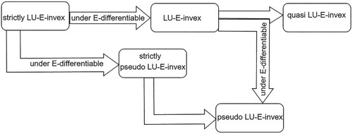
Note that every strictly pseudo E-invex interval-valued function is pseudo E-invex interval-valued function and every weakly E-differentiable pseudo E-convex interval-valued function is pseudo E-invex interval-valued function. Also, every pseudo E-convex interval-valued function is E-invex interval-valued function and every E-invex interval-valued function is pseudo E-invex interval-valued function for the same function η. Further, weakly E-differentiable quasi E-convex interval-valued function is trivially quasi E-invex interval-valued function and every pseudo E-invex interval-valued function is quasi E-invex interval-valued function, but the converse is not true (see Figure 2).

Figure 2. Relationships between E-differentiable LU-E-invexity and different types of E-differentiable generalized LU-E-invexity.

3. E-differentiable interval-valued optimization problems

In the paper, consider the following (not necessarily differentiable) interval-valued multiobjective programming problem with both inequality and equality constraints: $\begin{array}{r}\begin{array}{rl}& \mathrm{minimize}f(x)=(f_1\left(x\right),\dots ,f_p\left(x\right))\\ & \mathrm{subject}\mathrm{to}{g}_k(x)\leqq 0,k\in K=\{1,\dots ,m\},\\ & h_t(x)=0,t\in T=\{1,\dots ,s\},\\ & x\in R^n,\end{array}\mathrm{IVP}\end{array}$where each $f_i:R^n\to {\mathcal{K}}_C$, $i\in I=\{1,\dots ,p\}$, is an interval-valued function defined on $R^n$, that is, $f_i(x)=[f_i^L(x),f_i^U(x)]$, and, moreover, each function $g_k:R^n\to R$, $k\in K$ and each function $h_t:R^n\to R$, $t\in T$, are real-valued functions defined on $R^n$.

For the purpose of simplifying our presentation, we will next introduce some notations which will be used frequently throughout this paper. We will write $g:=(g_1,\dots ,g_m):R^n\to R^m$ and $h:=(h_1,\dots ,h_s):R^n\to R^s$ for convenience. Let $\mathrm{\Omega }:=\{x\in R^n:g_k(x)\leqq 0,k\in K,h_t(x)=0,t\in T\}$be the set of all feasible solutions of (IVP).

Definition 3.1

[32]

Let $x^{\ast }$ be a feasible solution of (IVP). We say that $x^{\ast }$ is

1. a weak LU-Pareto (weakly LU-efficient) solution of (IVP) if and only if there exists no other feasible point $x$ such that, for each $i\in I$, $f_i(x){<}_{LU}{f}_i(x^{\ast }).$

2. a LU-Pareto (LU-efficient) solution of (IVP) if and only if there exists no other feasible point $x$ such that $f(x){<}_{LU}f(x^{\ast }).$

Definition 3.2

[8]

Let $x^{\ast }$ be a feasible solution of (IVP). We say that $x^{\ast }$ is

1. a weak LS-Pareto (weakly LS-efficient) solution of (IVP) if and only if there exists no other feasible point $x$ such that, for each $i\in I$, $f_i(x){<}_{LS}{f}_i(x^{\ast }).$

2. an LS-Pareto (LS-efficient) solution of (IVP) if and only if there exists no other feasible point $x$ such that $f(x){<}_{LS}f(x^{\ast }).$

Remark 3.1

[32]

Let us denote by ${\mathrm{\Omega }}_P^{LU}$ and ${\mathrm{\Omega }}_{WP}^{LU}$ the set of LU-Pareto optimal solutions and weakly LU-Pareto optimal solutions, respectively. Then ${\mathrm{\Omega }}_P^{LU}\subseteq {\mathrm{\Omega }}_{WP}^{LU}$.

Remark 3.2

[27]

Let us denote by ${\mathrm{\Omega }}_P^{LS}$ and ${\mathrm{\Omega }}_{WP}^{LS}$ the set of LS-Pareto optimal solutions and weakly LS-Pareto optimal solutions, respectively. Then ${\mathrm{\Omega }}_P^{LS}\subseteq {\mathrm{\Omega }}_{WP}^{LS}$.

Further, let $E:R^n\to R^n$ be a given one-to-one and onto operator. Throughout the paper, we shall assume that the functions constituting the problem (IVP) are weakly E-differentiable. Therefore, for the considered interval-valued multiobjective programming problem (IVP), we construct the following associated vector optimization problem (IVP${}_E$) with the multiple interval-valued objective function: $\begin{array}{r}\begin{array}{rl}& \mathrm{minimize}f(E\left(x\right))=(f_1\left(E\left(x\right)\right),\dots ,f_p\left(E\left(x\right)\right))\\ & \mathrm{subject}\mathrm{to}{g}_k(E\left(x\right))\leqq 0,k\in K=\{1,\dots ,m\},\\ & h_t(E\left(x\right))=0,t\in T=\{1,\dots ,s\},\\ & x\in R^n,\end{array}{\mathrm{IVP}}_E\end{array}$where the functions $f_i$, $i\in I$, $g_k$, $k\in K$, $h_t$, $t\in T$, are defined in the similar way as for (IVP). We call (IVP${}_E$) the E-vector optimization problem with the multiple interval-valued objective function or the interval-valued E-vector optimization problem. Let ${\mathrm{\Omega }}_E$ be the set of all feasible solutions of (IVP${}_E$), that is, ${\mathrm{\Omega }}_E:=\{x\in R^n:g_k(E\left(x\right))\leqq 0,k\in K,h_t(E\left(x\right))=0,t\in T\}.$

Definition 3.3

[5]

Let $x^{\ast }$ be a feasible solution of (IVP${}_E$). We say that $E(x^{\ast })$ is

1. a weak LU-E-Pareto (weakly LU-E-efficient) solution of (IVP) if and only if there is no other feasible solution $E(x)$ such that, for each $i\in I$, $f_i(E(x)){<}_{LU}{f}_i(E(x^{\ast })).$

2. a LU-E-Pareto (LU-E-efficient) solution of (IVP) if and only if there is no other feasible solution $E(x)$ such that $f(E(x)){<}_{LU}f(E(x^{\ast })).$

Definition 3.4

Let $x^{\ast }$ be a feasible solution of (IVP${}_E$). We say that $E(x^{\ast })$ is

1. a weak LS-E-Pareto (weakly LS-E-efficient) solution of (IVP) if and only if there is no other feasible solution $E(x)$ such that, for each $i\in I$, $f_i(E(x)){<}_{LS}{f}_i(E(x^{\ast })).$

2. a LS-E-Pareto (LS-E-efficient) solution of (IVP) if and only if there is no other feasible solution $E(x)$ such that $f(E(x)){<}_{LS}f(E(x^{\ast })).$

Lemma 3.5

[4]

Let $E:R^n\to R^n$ be an one-to-one and onto operator. Then $E({\mathrm{\Omega }}_E)=\mathrm{\Omega }$.

Remark 3.3

Let us denote by ${\mathrm{\Omega }}_{EP}^{LU}$ and ${\mathrm{\Omega }}_{WEP}^{LU}$ the set of LU-E-Pareto optimal solutions and weakly LU-E-Pareto optimal solutions, respectively. Then ${\mathrm{\Omega }}_{EP}^{LU}\subseteq {\mathrm{\Omega }}_{WEP}^{LU}$.

Remark 3.4

Let us denote by ${\mathrm{\Omega }}_{EP}^{LS}$ and ${\mathrm{\Omega }}_{WEP}^{LS}$ the set of LS-E-Pareto optimal solutions and weakly LS-E-Pareto optimal solutions, respectively. Then ${\mathrm{\Omega }}_{EP}^{LS}\subseteq {\mathrm{\Omega }}_{WEP}^{LS}$.

Theorem 3.6

Let $E:R^n\to R^n$ be a one-to-one and onto operator and ${\mathrm{\Omega }}_E$ be a feasible set of (IVP${}_E$). Then

(i)	${\mathrm{\Omega }}_{EP}^{LU}\subseteq {\mathrm{\Omega }}_{EP}^{LS}$,
(ii)	${\mathrm{\Omega }}_{WEP}^{LU}\subseteq {\mathrm{\Omega }}_{WEP}^{LS}$.

Proof.

Let $x^{\ast }\in {\mathrm{\Omega }}_E$ be the feasible of (IVP${}_E$).

1. Assume that $x^{\ast }\in {\mathrm{\Omega }}_{EP}^{LU}$ is an LU-E-Pareto solution of the problem (IVP${}_E$). Suppose, contrary to the result, that $x^{\ast }\notin {\mathrm{\Omega }}_{EP}^{LS}$. Then, by Definition 3.3(ii), there exists $x^{\circ }$ such that $f(E(x^{\circ })){<}_{LS}f(E(x^{\ast }))$. By Proposition 2.2, we have that $f(E(x^{\circ })){<}_{LU}f(E(x^{\ast }))$, contradicting the assumption that $x^{\ast }\in {\mathrm{\Omega }}_{EP}^{LU}$ is an LU-E-Pareto solution of the problem (IVP${}_E$). Hence, ${\mathrm{\Omega }}_{EP}^{LU}\subseteq {\mathrm{\Omega }}_{EP}^{LS}$.

2. Assume that $x^{\ast }\in {\mathrm{\Omega }}_{WEP}^{LU}$ is a weakly LU-E-Pareto solution of the problem (IVP${}_E$). Suppose, contrary to the result, that $x^{\ast }\notin {\mathrm{\Omega }}_{WEP}^{LS}$. Then, by Definition 3.4(i), there exists $x^{\circ }$ such that, for each $i\in I$, $f_i(E(x^{\circ })){<}_{LS}{f}_i(E(x^{\ast }))$. By Proposition 2.2, we have that, for each $i\in I$, $f_i(E(x^{\circ })){<}_{LU}{f}_i(E(x^{\ast }))$, contradicting the assumption that $x^{\ast }\in {\mathrm{\Omega }}_{WEP}^{LU}$ is a weakly LU-E-Pareto solution of the problem (IVP${}_E$). Hence, ${\mathrm{\Omega }}_{WEP}^{LU}\subseteq {\mathrm{\Omega }}_{WEP}^{LS}$.

Lemma 3.7

[5]

Let $E:R^n\to R^n$ be a one-to-one and onto operator and let $z^{\ast }\in {\mathrm{\Omega }}_E$ be a weak LU-Pareto solution (a LU-Pareto solution) of the interval-valued problem (IVP${}_E$). Then $E(z^{\ast })$ is a weak LU-Pareto solution (an LU-Pareto solution) of the problem (IVP).

Now, we prove the relationship between (weak) LS-Pareto optimal solutions in both interval-valued vector optimization problems (IVP) and (IVP${}_E$).

Lemma 3.8

Let $E:R^n\to R^n$ be a one-to-one and onto operator and $x^{\ast }\in \mathrm{\Omega }$ be a weak LS-Pareto solution (an LS-Pareto solution) of the problem (IVP). Then, there exists $z^{\ast }\in {\mathrm{\Omega }}_E$ such that $x^{\ast }=E(z^{\ast })$ and $z^{\ast }$ is a weak LS-Pareto solution (an LS-Pareto solution) of the problem (IVP${}_E$).

Proof.

Let $x^{\ast }\in \mathrm{\Omega }$ be a weak LS-Pareto solution for (IVP). Moreover, $E:R^n\to R^n$ is assumed to be a one-to-one and onto operator. Hence, by Lemma 3.5, there exists $z^{\ast }\in {\mathrm{\Omega }}_E$ such that $x^{\ast }=E(z^{\ast })$. Now, we prove that $z^{\ast }$ is a weak LS-Pareto solution of the problem (IVP${}_E$). By means of contradiction, suppose that $z^{\ast }$ is not a weak LS-Pareto solution of the problem (IVP${}_E$). Then, by the definition of a weak LS-Pareto solution, there exists $z^{\circ }\in {\mathrm{\Omega }}_E$ such that $(f\circ E)(z^{\circ }){<}_{LS}(f\circ E)(z^{\ast })$. Hence, by the definition of the relation ${<}_{LS}$, it follows that, for any $i\in I$, $\begin{array}{rl}& (f_i^L(E(z^{\circ }))<f_i^L(E\left(z^{\ast }\right))\wedge f_i^S(E(z^{\circ }))\leqq f_i^S(E\left(z^{\ast }\right)))\\ & \mathrm{or}(f_i^L(E(z^{\circ }))\leqq f_i^L(E\left(z^{\ast }\right))\wedge f_i^S(E(z^{\circ }))<f_i^S(E\left(z^{\ast }\right)))\\ & \mathrm{or}(f_i^L(E(z^{\circ }))<f_i^L(E\left(z^{\ast }\right))\wedge f_i^S(E(z^{\circ }))<f_i^S(E\left(z^{\ast }\right))).\end{array}$By Lemma 3.5, we have that there exists $x^{\circ }\in \mathrm{\Omega }$ such that $x^{\circ }=E(z^{\circ })$. Taking also that $x^{\ast }=E(z^{\ast })$, the above inequalities yield, respectively, (36) $\begin{array}{rl}& (f_i^L(x^{\circ })<f_i^L(x^{\ast })\wedge f_i^S(x^{\circ })\leqq f_i^S(x^{\ast }))\\ & \mathrm{or}(f_i^L(x^{\circ })\leqq f_i^L(x^{\ast })\wedge f_i^S(x^{\circ })<f_i^S(x^{\ast }))\\ & \mathrm{or}(f_i^L(x^{\circ })<f_i^L(x^{\ast })\wedge f_i^S(x^{\circ })<f_i^S(x^{\ast })).\end{array}$(36) Hence, by the definition of the relation ${<}_{LS}$, inequalities (36(36) $\begin{array}{rl}& (f_i^L(x^{\circ })<f_i^L(x^{\ast })\wedge f_i^S(x^{\circ })\leqq f_i^S(x^{\ast }))\\ & \mathrm{or}(f_i^L(x^{\circ })\leqq f_i^L(x^{\ast })\wedge f_i^S(x^{\circ })<f_i^S(x^{\ast }))\\ & \mathrm{or}(f_i^L(x^{\circ })<f_i^L(x^{\ast })\wedge f_i^S(x^{\circ })<f_i^S(x^{\ast })).\end{array}$(36) ) imply that the inequality $f(x^{\circ }){<}_{LS}f(x^{\ast })$ is fulfilled, which is a contradiction to weakly LS-efficiency of $x^{\ast }$ for the problem (IVP). The proof for the case, in which $x^{\ast }\in \mathrm{\Omega }$ is an LS-Pareto solution of the problem (IVP), is analogous and, therefore, it is omitted.

Lemma 3.9

Let $E:R^n\to R^n$ be a one-to-one and onto operator and let $z^{\ast }\in {\mathrm{\Omega }}_E$ be a weak LS-Pareto solution (a LS-Pareto solution) of the interval-valued problem (IVP${}_E$). Then $E(z^{\ast })$ is a weak LS-Pareto solution (an LS-Pareto solution) of the problem (IVP).

Proof.

Assume that $z^{\ast }\in {\mathrm{\Omega }}_E$ is a weak LS-Pareto solution of the problem (IVP${}_E$). Note that, by Lemma 3.5, $E(z^{\ast })\in \mathrm{\Omega }$. We proceed by contradiction. Suppose, contrary to the result, that $E(z^{\ast })$ is not a weak LS-Pareto solution of the problem (IVP). Then, by Definition 3.1(i), there exists $x^{\circ }\in \mathrm{\Omega }$ such that $f_i(x^{\circ }){<}_{LS}{f}_i(E(z^{\ast }))$ for each $i\in I$. Hence, by Lemma 3.5, there exists $z^{\circ }\in {\mathrm{\Omega }}_E$ such that $x^{\circ }=E(z^{\circ })$. Thus, the inequality above implies that $(f_i\circ E)(z^{\circ }){<}_{LS}(f_i\circ E)(z^{\ast })$ for each $i\in I$, which is a contradiction to weakly LS-efficiency of $z^{\ast }$ for the problem (VP${}_E$). The proof when it is assumed that $z^{\ast }\in {\mathrm{\Omega }}_E$ is an LS-Pareto solution of the problem (VP${}_E$) is similar and, therefore, it is omitted.

Theorem 3.10

Let $E:R^n\to R^n$ and $z^{\ast }\in {\mathrm{\Omega }}_E$ be a feasible solution of (IVP${}_E$). If $z^{\ast }\in {\mathrm{\Omega }}_E$ be a weak LU-Pareto solution (an LU-Pareto solution) of the problem (IVP${}_E$), then $z^{\ast }$ is a weak LS-Pareto solution ( an LS-Pareto solution) of the problem (IVP${}_E$).

Proof.

Suppose that $z^{\ast }\in {\mathrm{\Omega }}_E$ is not a weak LS-Pareto solution (an LS-Pareto solution) of the problem (IVP${}_E$). Then there exists $z\in {\mathrm{\Omega }}_E$ such that $f_i(E(z)){<}_{LS}{f}_i(E(z^{\ast }))$ for each $i\in I$ ($f(E(z)){<}_{LS}f(E(z^{\ast }))$). From Proposition 2.2, we have that $f_i(E(z)){<}_{LU}{f}_i(E(z^{\ast }))$ for each $i\in I$ ($f(E(z)){<}_{LU}f(E(z^{\ast }))$) which is a contradiction with the hypothesis of the theorem.

Theorem 3.11

[5]

Let $x^{\ast }\in {\mathrm{\Omega }}_E$ be a weak LU-Pareto solution of the (IVP${}_E$) (and, thus, $E(x^{\ast })$ be a weak LU-E-Pareto solution of the problem (IVP)). Further, assume that the E-Kuhn–Tucker constraint qualification introduced by Antczak and Abdulaleem [5] is satisfied at $x^{\ast }$. Then there exist ${{\lambda }^{\ast }}^L\in R^p$, ${{\lambda }^{\ast }}^U\in R^p$, ${\mu }^{\ast }\in R^m$ and ${\zeta }^{\ast }\in R^s$ such that (37) $\begin{array}{rl}& \sum _{i=1}^p{{\lambda }_i^{\ast }}^L\mathrm{\nabla }(f_i^L\circ E)(x^{\ast })+\sum _{i=1}^p{{\lambda }_i^{\ast }}^U\mathrm{\nabla }(f_i^U\circ E)(x^{\ast })\\ & +\sum _{k=1}^m{\mu }_k^{\ast }\mathrm{\nabla }(g_k\circ E)(x^{\ast })+\sum _{t=1}^s{\zeta }_t^{\ast }\mathrm{\nabla }(h_t\circ E)(x^{\ast })=0,\end{array}$(37) (38) $\begin{array}{rl}& {\mu }_k^{\ast }(g_k\circ E)(x^{\ast })=0,k\in K,\end{array}$(38) (39) $\begin{array}{rl}& ({{\lambda }^{\ast }}^L,{{\lambda }^{\ast }}^U)\ge 0,{\mu }^{\ast }\geqq 0.\end{array}$(39)

Definition 3.12

[21]

Let $Y\subseteq R^p$. It is said that $z\in R^p$ is a convergence vector for Y at $y^{\ast }\in Y$ if there exist a sequence $\{y_j\}$ in Y and a sequence $\{{\rho }_j\}$ of strictly positive real numbers such that $\underset{j\to \mathrm{\infty }}{lim}{y}_j=y^{\ast },\underset{j\to \mathrm{\infty }}{lim}{\rho }_j=0,\underset{j\to \mathrm{\infty }}{lim}\frac{y_j-y^{\ast }}{{\rho }_j}=z.$

Theorem 3.13

Let $E:R^n\to R^n$, $f_i:R^n\to {\mathcal{K}}_C,i\in I$ and ${\mathrm{\Omega }}_E\subset R^n$. If $x^{\ast }\in {\mathrm{\Omega }}_E$ is a weak LS-Pareto solution for $f\circ E$ on ${\mathrm{\Omega }}_E$ (and, thus, $E(x^{\ast })\in \mathrm{\Omega }$ is a weak LS-E-Pareto solution for f on Ω), then no a convergence vector for $f({\mathrm{\Omega }}_E)$ at $y^{\ast }=f(E(x^{\ast }))$ is strictly negative.

Proof.

$x^{\ast }\in {\mathrm{\Omega }}_E$ is a weak LS-Pareto solution for $f\circ E$ on ${\mathrm{\Omega }}_E$ (and, thus, $E(x^{\ast })\in \mathrm{\Omega }$ is a weak LS-E-Pareto solution for f on Ω). Hence, $y^{\ast }=({y^{\ast }}^L,{y^{\ast }}^S)=(f^L(E(x^{\ast })),f^S(E(x^{\ast })))$ is a weak LS-Pareto solution for the set $f({\mathrm{\Omega }}_E)=(f^L({\mathrm{\Omega }}_E),f^S({\mathrm{\Omega }}_E))$. Let $d\in R^n$ be a convergence vector for ${\mathrm{\Omega }}_E$ at $x^{\ast }$. Further, let $\{x_j\}\subset {\mathrm{\Omega }}_E$ be the corresponding sequence converging to $x^{\ast }$. Consider a sequence $\{y_j\}\subset f({\mathrm{\Omega }}_E)=(f^L({\mathrm{\Omega }}_E),f^S({\mathrm{\Omega }}_E))$, that is, $y_j=(y_j^L,y_j^S)$ such that $y_j^L=f^L(E(x_j))$ and $y_j^S=f^S(E(x_j))$ for any integer. This means that $\{y_j^L\}\subset f^L({\mathrm{\Omega }}_E)$ and $\{y_j^S\}\subset f^S({\mathrm{\Omega }}_E)$ for any integer. Since f is weakly E-differentiable at $x^{\ast }$, by Definitions 2.5 and 2.7, we have that the functions $f^L$ and $f^S$ are E-differentiable at $x^{\ast }$. By the differentiability of $f^L\circ E$ and $f^S\circ E$ at $x^{\ast }$, it follows that $f^L\circ E$ and $f^S\circ E$ are continuous at $x^{\ast }$. Thus the sequence $\{y_j\}$ is convergent to $y^{\ast }=f(E(x^{\ast }))$, which means that the sequences $\{y_j^L\}$ and $\{y_j^S\}$ are convergent to ${y^{\ast }}^L=f^L(E(x^{\ast }))$ and ${y^{\ast }}^S=f^S(E(x^{\ast }))$, respectively. By means of contradiction, suppose that there exists a convergence vector $z^{\ast }=({z^{\ast }}^L,{z^{\ast }}^S)$ for $f({\mathrm{\Omega }}_E)=(f^L({\mathrm{\Omega }}_E),f^S({\mathrm{\Omega }}_E))$ at $y^{\ast }=({y^{\ast }}^L,{y^{\ast }}^S)=(f^L(E(x^{\ast })),f^S(E(x^{\ast })))=f(E(x^{\ast }))$, which is a strictly negative. Then, by Definition 3.12, it follows that, for the sequence $\{y_j\}\subset f({\mathrm{\Omega }}_E)$, $\underset{j\to \mathrm{\infty }}{lim}{y}_j=y^{\ast }$, there exists a sequence of strictly positive real numbers $\{{\rho }_j\}$ converging to 0 such that (40) $\underset{j\to \mathrm{\infty }}{lim}\frac{y_j-y^{\ast }}{{\rho }_j}=z^{\ast }.$(40) Since $y_j=f(E(x_j))$ for any integer and $y^{\ast }=f(E(x^{\ast }))$, gives (41) $\underset{j\to \mathrm{\infty }}{lim}\frac{f(E(x_j))-f(E(x^{\ast }))}{{\rho }_j}=z^{\ast }.$(41) Using $f(E(x^{\ast }))=(f^L(E(x^{\ast })),f^S(E(x^{\ast })))$, $f(E(x_j))=(f^L(E(x_j)),f^S(E(x_j)))$ and $z^{\ast }=({z^{\ast }}^L,{z^{\ast }}^S)$, (41(41) $\underset{j\to \mathrm{\infty }}{lim}\frac{f(E(x_j))-f(E(x^{\ast }))}{{\rho }_j}=z^{\ast }.$(41) ) yields (42) $\begin{array}{rl}& \underset{j\to \mathrm{\infty }}{lim}\frac{f^L(E(x_j))-f^S(E(x^{\ast }))}{{\rho }_j}={z^{\ast }}^L,\end{array}$(42) (43) $\begin{array}{rl}& \underset{j\to \mathrm{\infty }}{lim}\frac{f^S(E(x_j))-f^L(E(x^{\ast }))}{{\rho }_j}={z^{\ast }}^S.\end{array}$(43) By assumption, $z^{\ast }=({z^{\ast }}^L,{z^{\ast }}^S)<0$. Hence, (42(42) $\begin{array}{rl}& \underset{j\to \mathrm{\infty }}{lim}\frac{f^L(E(x_j))-f^S(E(x^{\ast }))}{{\rho }_j}={z^{\ast }}^L,\end{array}$(42) )–(43(43) $\begin{array}{rl}& \underset{j\to \mathrm{\infty }}{lim}\frac{f^S(E(x_j))-f^L(E(x^{\ast }))}{{\rho }_j}={z^{\ast }}^S.\end{array}$(43) ) imply, respectively, (44) $\begin{array}{rl}& \underset{j\to \mathrm{\infty }}{lim}\frac{f^L(E(x_j))-f^S(E(x^{\ast }))}{{\rho }_j}<0,\end{array}$(44) (45) $\begin{array}{rl}& \underset{j\to \mathrm{\infty }}{lim}\frac{f^S(E(x_j))-f^L(E(x^{\ast }))}{{\rho }_j}<0.\end{array}$(45) Since $\{{\rho }_j\}$ is a sequence of strictly positive real numbers for any integer, for each $i\in I$, there exist $J_i^L$ and $J_i^S$ such that (46) $\begin{array}{rl}& f_i^L(E(x_j))<f_i^S(E(x^{\ast }))\mathrm{for}\mathrm{any}j>J_i^L,\end{array}$(46) (47) $\begin{array}{rl}& f_i^S(E(x_j))<f_i^L(E(x^{\ast }))\mathrm{for}\mathrm{any}j>J_i^S.\end{array}$(47) By Definition 2.4, it follows that (48) $\begin{array}{rl}& f_i^L(E(x^{\ast }))\leqq f_i^S(E(x^{\ast })),i\in I,\end{array}$(48) (49) $\begin{array}{rl}& f_i^L(E(x_j))\leqq f_i^S(E(x_j)),i\in I.\end{array}$(49) Combining (47(47) $\begin{array}{rl}& f_i^S(E(x_j))<f_i^L(E(x^{\ast }))\mathrm{for}\mathrm{any}j>J_i^S.\end{array}$(47) ), (48(48) $\begin{array}{rl}& f_i^L(E(x^{\ast }))\leqq f_i^S(E(x^{\ast })),i\in I,\end{array}$(48) ) and (49(49) $\begin{array}{rl}& f_i^L(E(x_j))\leqq f_i^S(E(x_j)),i\in I.\end{array}$(49) ), we get (50) $\begin{array}{rl}& f_i^L(E(x_j))<f_i^L(E(x^{\ast }))\mathrm{for}\mathrm{any}j>max\{J_i^L,J_i^S\},\end{array}$(50) (51) $\begin{array}{rl}& f_i^S(E(x_j))<f_i^S(E(x^{\ast }))\mathrm{for}\mathrm{any}j>max\{J_i^L,J_i^S\}.\end{array}$(51) Let $J_{max}=max\{J_i^L,J_i^S:i\in I\}$. Then, (50(50) $\begin{array}{rl}& f_i^L(E(x_j))<f_i^L(E(x^{\ast }))\mathrm{for}\mathrm{any}j>max\{J_i^L,J_i^S\},\end{array}$(50) ) and (51(51) $\begin{array}{rl}& f_i^S(E(x_j))<f_i^S(E(x^{\ast }))\mathrm{for}\mathrm{any}j>max\{J_i^L,J_i^S\}.\end{array}$(51) ) imply, respectively, $\begin{array}{rl}& f_i^L(E(x_j))<f_i^L(E(x^{\ast }))\mathrm{for}\mathrm{any}j>J_{max},i\in I,\\ & f_i^S(E(x_j))<f_i^S(E(x^{\ast }))\mathrm{for}\mathrm{any}j>J_{max},i\in I\end{array}$where $x_j\in {\mathrm{\Omega }}_E$. This is a contradiction (for any sufficiently large j) to the assumption that $x^{\ast }\in {\mathrm{\Omega }}_E$ is a weak LS-Pareto solution for $f\circ E$ on ${\mathrm{\Omega }}_E$ and, thus, $E(x^{\ast })\in \mathrm{\Omega }$ is a weak LS-E-Pareto solution for f on Ω. Thus the proof of this theorem is completed.

Theorem 3.14

E-Karush–Kuhn–Tucker (E-KKT) necessary optimality conditions

Let $x^{\ast }\in {\mathrm{\Omega }}_E$ be a weak LS-Pareto solution of the problem (IVP${}_E$) (and, thus, $E(x^{\ast })$ be a weak LS-E-Pareto solution of the problem (IVP)). Further, assume that the E-Guignard constraint qualification (GCQ${}_E$) introduced by Abdulaleem [2] is satisfied at $x^{\ast }$. Then there exist ${{\lambda }^{\ast }}^L\in R^p$, ${{\lambda }^{\ast }}^S\in R^p$, ${\mu }^{\ast }\in R^m$ and ${\zeta }^{\ast }\in R^s$ such that (52) $\begin{array}{rl}& \sum _{i=1}^p{{\lambda }_i^{\ast }}^L\mathrm{\nabla }(f_i^L\circ E)(x^{\ast })+\sum _{i=1}^p{{\lambda }_i^{\ast }}^S\mathrm{\nabla }(f_i^S\circ E)(x^{\ast })\\ & +\sum _{k=1}^m{\mu }_k^{\ast }\mathrm{\nabla }(g_k\circ E)(x^{\ast })+\sum _{t=1}^s{\zeta }_t^{\ast }\mathrm{\nabla }(h_t\circ E)(x^{\ast })=0,\end{array}$(52) (53) $\begin{array}{rl}& {\mu }_k^{\ast }(g_k\circ E)(x^{\ast })=0,k\in K,\end{array}$(53) (54) $\begin{array}{rl}& ({{\lambda }^{\ast }}^L,{{\lambda }^{\ast }}^S)\ge 0,{\mu }^{\ast }\geqq 0.\end{array}$(54)

Proof.

Let $x^{\ast }\in {\mathrm{\Omega }}_E$ be a weak LS-Pareto solution of the problem (IVP${}_E$). Hence, by Lemma 3.7, $E(x^{\ast })$ is a (weak) LS-E-Pareto solution of the problem (IVP). Further, assume that the E-Guignard constraint qualification (GCQ${}_E$) introduced by Abdulaleem [2] is satisfied at $x^{\ast }$. Therefore, $y^{\ast }=({y^{\ast }}^L,{y^{\ast }}^S)=(f^L(E(x^{\ast })),f^{S}E((x^{\ast })))$ is a weak LS-Pareto solution for the set $f({\mathrm{\Omega }}_E)=(f^L({\mathrm{\Omega }}_E),f^S({\mathrm{\Omega }}_E))$. Let $d\in R^n$ be a convergence vector for the set ${\mathrm{\Omega }}_E$ at $x^{\ast }$. Further, let $\{x_j\}\subset {\mathrm{\Omega }}_E$, $\{{\rho }_j\}$ be the corresponding sequences, where $\{{\rho }_j\}$ is a sequence of strictly positive real numbers. Then, we consider the sequences $\{y_j^L\}\subset f^L({\mathrm{\Omega }}_E)$ and $\{y_j^S\}\subset f^S({\mathrm{\Omega }}_E)$ such that $y_j^L=f^L(E(x_j))$ and $y_j^S=f^S(E(x_j))$. By assumption, $f=(f^L,f^S)$ is weakly E-differentiable at $x^{\ast }$. Thus, by Definition 2.7, it follows that $f^L\circ E$ and $f^S\circ E$ are differentiable at $x^{\ast }$. Hence, they are continuous at $x^{\ast }$. Then, by the continuity of $f^L\circ E$ and $f^S\circ E$ at $x^{\ast }$, the sequences $\{y_j^L\}$ and $\{y_j^S\}$ are convergent to ${y^{\ast }}^L$ and ${y^{\ast }}^S$, respectively. By Definition 2.7, we have (55) $\begin{array}{rl}& f^L(E(x_j))=f^L(E(x^{\ast }))+\mathrm{\nabla }{f}^L(E(x^{\ast }){)}^T(x_j-x^{\ast })+{\theta }^L(x^{\ast },x_j-x^{\ast })\Vert x_j-x^{\ast }\Vert ,\end{array}$(55) (56) $\begin{array}{rl}& f^S(E(x_j))=f^S(E(x^{\ast }))+\mathrm{\nabla }{f}^S(E(x^{\ast }){)}^T(x_j-x^{\ast })+{\theta }^S(x^{\ast },x_j-x^{\ast })\Vert x_j-x^{\ast }\Vert ,\end{array}$(56) where ${\theta }^L(x^{\ast },x_j-x^{\ast })\to 0$, ${\theta }^S(x^{\ast },x_j-x^{\ast })\to 0$, when $x_j\to x^{\ast }.$ Then, we have (57) $\begin{array}{rl}\frac{y_j^L-{y^{\ast }}^L}{{\rho }_j}& =\frac{f^L(E(x_j))-f^L(E(x^{\ast }))}{{\rho }_j}\\ & =\mathrm{\nabla }{f}^L(E(x^{\ast }){)}^T\left(\frac{x_j-x^{\ast }}{{\rho }_j}\right)+{\theta }^L(x^{\ast },x_j-x^{\ast })\frac{\Vert x_j-x^{\ast }\Vert }{{\rho }_j},\end{array}$(57) (58) $\begin{array}{rl}\frac{y_j^S-{y^{\ast }}^S}{{\rho }_j}& =\frac{f^S(E(x_j))-f^S(E(x^{\ast }))}{{\rho }_j}\\ & =\mathrm{\nabla }{f}^S(E(x^{\ast }){)}^T\left(\frac{x_j-x^{\ast }}{{\rho }_j}\right)+{\theta }^S(x^{\ast },x_j-x^{\ast })\frac{\Vert x_j-x^{\ast }\Vert }{{\rho }_j}.\end{array}$(58) By (57(57) $\begin{array}{rl}\frac{y_j^L-{y^{\ast }}^L}{{\rho }_j}& =\frac{f^L(E(x_j))-f^L(E(x^{\ast }))}{{\rho }_j}\\ & =\mathrm{\nabla }{f}^L(E(x^{\ast }){)}^T\left(\frac{x_j-x^{\ast }}{{\rho }_j}\right)+{\theta }^L(x^{\ast },x_j-x^{\ast })\frac{\Vert x_j-x^{\ast }\Vert }{{\rho }_j},\end{array}$(57) ), (58(58) $\begin{array}{rl}\frac{y_j^S-{y^{\ast }}^S}{{\rho }_j}& =\frac{f^S(E(x_j))-f^S(E(x^{\ast }))}{{\rho }_j}\\ & =\mathrm{\nabla }{f}^S(E(x^{\ast }){)}^T\left(\frac{x_j-x^{\ast }}{{\rho }_j}\right)+{\theta }^S(x^{\ast },x_j-x^{\ast })\frac{\Vert x_j-x^{\ast }\Vert }{{\rho }_j}.\end{array}$(58) ) and Definition 3.12, we conclude that the vectors $z^L$ and $z^S$ defined by $\begin{array}{rl}{z}^L& =\underset{j\to \mathrm{\infty }}{lim}\frac{y_j^L-{y^{\ast }}^L}{{\rho }_j}=\mathrm{\nabla }{f}^L(E(x^{\ast }){)}^{T}d,\\ z^S& =\underset{j\to \mathrm{\infty }}{lim}\frac{y_j^S-{y^{\ast }}^S}{{\rho }_j}=\mathrm{\nabla }{f}^S(E(x^{\ast }){)}^{T}d\end{array}$are convergence vectors for $f^L({\mathrm{\Omega }}_E)$ and $f^S({\mathrm{\Omega }}_E)$, respectively. By the constraint qualification, it follows that $d\in R^n$ is a convergence for the set ${\mathrm{\Omega }}_E$ if and only if d is a solution to the following system: (59) $\begin{array}{rl}\mathrm{\nabla }{g}_k{(E(x^{\ast }))}^{T}d& \leqq 0,k\in K(E(x^{\ast })),\end{array}$(59) (60) $\begin{array}{rl}\mathrm{\nabla }{h}_t(E(x^{\ast }){)}^{T}d& =0,t\in T.\end{array}$(60) Since $x^{\ast }\in {\mathrm{\Omega }}_E$ be a weak LS-Pareto solution of the problem (IVP${}_E$) and, thus, $E(x^{\ast })$ is a (weak) LS-E-Pareto solution of the problem (IVP), by Theorem 3.13, we have that there is no a strictly negative convergence vector for the set $f({\mathrm{\Omega }}_E)=(f^L({\mathrm{\Omega }}_E),f^S({\mathrm{\Omega }}_E))$ at $y^{\ast }$. Therefore, the system (61) $\begin{array}{rl}& \mathrm{\nabla }{f}_i^L(E(x^{\ast }){)}^{T}d<0,\mathrm{\nabla }{f}_i^S(E(x^{\ast }){)}^{T}d<0,i\in I,\end{array}$(61) (62) $\begin{array}{rl}& \mathrm{\nabla }{g}_k(E(x^{\ast }){)}^{T}d\leqq 0,k\in K(E(x^{\ast })),\end{array}$(62) (63) $\begin{array}{rl}& \mathrm{\nabla }{h}_t(E(x^{\ast }){)}^{T}d=0,t\in T\end{array}$(63) has no a solution $d\in R^n$. Therefore, by Motzkin's theorem of the alternative introduced by Mangasarian [22], there exist ${{\lambda }^{\ast }}^L\in R^p$, ${{\lambda }^{\ast }}^S\in R^p$, $({{\lambda }^{\ast }}^L,{{\lambda }^{\ast }}^S)\ge 0$, ${\mu }_k^{\ast }$, $k\in K(E(x^{\ast }))$, and ${\zeta }^{\ast }\in R^s$ such that (64) $\begin{array}{rl}& \sum _{i=1}^p{{\lambda }_i^{\ast }}^L\mathrm{\nabla }(f_i^L\circ E)(x^{\ast })+\sum _{i=1}^p{{\lambda }_i^{\ast }}^S\mathrm{\nabla }(f_i^S\circ E)(x^{\ast })\\ & +\sum _{k\in K\left(E\left(x^{\ast }\right)\right)}{\mu }_k^{\ast }\mathrm{\nabla }(g_k\circ E)(x^{\ast })+\sum _{t=1}^s{\zeta }_t^{\ast }\mathrm{\nabla }(h_t\circ E)(x^{\ast })=0.\end{array}$(64) If we set ${\mu }_k^{\ast }=0$ for all $k\in K\mathrm{\setminus }K(E(x^{\ast }))$, then (64(64) $\begin{array}{rl}& \sum _{i=1}^p{{\lambda }_i^{\ast }}^L\mathrm{\nabla }(f_i^L\circ E)(x^{\ast })+\sum _{i=1}^p{{\lambda }_i^{\ast }}^S\mathrm{\nabla }(f_i^S\circ E)(x^{\ast })\\ & +\sum _{k\in K\left(E\left(x^{\ast }\right)\right)}{\mu }_k^{\ast }\mathrm{\nabla }(g_k\circ E)(x^{\ast })+\sum _{t=1}^s{\zeta }_t^{\ast }\mathrm{\nabla }(h_t\circ E)(x^{\ast })=0.\end{array}$(64) ) implies (52(52) $\begin{array}{rl}& \sum _{i=1}^p{{\lambda }_i^{\ast }}^L\mathrm{\nabla }(f_i^L\circ E)(x^{\ast })+\sum _{i=1}^p{{\lambda }_i^{\ast }}^S\mathrm{\nabla }(f_i^S\circ E)(x^{\ast })\\ & +\sum _{k=1}^m{\mu }_k^{\ast }\mathrm{\nabla }(g_k\circ E)(x^{\ast })+\sum _{t=1}^s{\zeta }_t^{\ast }\mathrm{\nabla }(h_t\circ E)(x^{\ast })=0,\end{array}$(52) ). Further, note that also the complementary slackness condition (53(53) $\begin{array}{rl}& {\mu }_k^{\ast }(g_k\circ E)(x^{\ast })=0,k\in K,\end{array}$(53) ) is satisfied. Indeed, if $g_k(E(x^{\ast }))<0$, then $k\in K\mathrm{\setminus }K(E(x^{\ast }))$ and ${\mu }_k^{\ast }=0$. Hence, the proof of this theorem is completed.

Definition 3.15

The point $(x^{\ast },{\lambda }^{\ast },{\mu }^{\ast },{\zeta }^{\ast })\in {\mathrm{\Omega }}_E\times R^{2p}\times R^m\times R^s$ is said to be an Karush–Kuhn–Tucker point (KKT point) for the E-vector optimization problem (IVP${}_E$) with the multiple interval-valued objective if the Karush–Kuhn–Tucker necessary optimality conditions (37(37) $\begin{array}{rl}& \sum _{i=1}^p{{\lambda }_i^{\ast }}^L\mathrm{\nabla }(f_i^L\circ E)(x^{\ast })+\sum _{i=1}^p{{\lambda }_i^{\ast }}^U\mathrm{\nabla }(f_i^U\circ E)(x^{\ast })\\ & +\sum _{k=1}^m{\mu }_k^{\ast }\mathrm{\nabla }(g_k\circ E)(x^{\ast })+\sum _{t=1}^s{\zeta }_t^{\ast }\mathrm{\nabla }(h_t\circ E)(x^{\ast })=0,\end{array}$(37) )–(39(39) $\begin{array}{rl}& ({{\lambda }^{\ast }}^L,{{\lambda }^{\ast }}^U)\ge 0,{\mu }^{\ast }\geqq 0.\end{array}$(39) ) (the Karush–Kuhn–Tucker necessary optimality conditions (52(52) $\begin{array}{rl}& \sum _{i=1}^p{{\lambda }_i^{\ast }}^L\mathrm{\nabla }(f_i^L\circ E)(x^{\ast })+\sum _{i=1}^p{{\lambda }_i^{\ast }}^S\mathrm{\nabla }(f_i^S\circ E)(x^{\ast })\\ & +\sum _{k=1}^m{\mu }_k^{\ast }\mathrm{\nabla }(g_k\circ E)(x^{\ast })+\sum _{t=1}^s{\zeta }_t^{\ast }\mathrm{\nabla }(h_t\circ E)(x^{\ast })=0,\end{array}$(52) )–(54(54) $\begin{array}{rl}& ({{\lambda }^{\ast }}^L,{{\lambda }^{\ast }}^S)\ge 0,{\mu }^{\ast }\geqq 0.\end{array}$(54) )) are satisfied at $x^{\ast }$ with ${\lambda }^{\ast }$, ${\mu }^{\ast }$, and ${\zeta }^{\ast }$.

Now, we prove the sufficiency of the E-KKT necessary optimality conditions for E-differentiable interval-valued vector optimization problem (IVP) under E-invexity hypotheses.

Theorem 3.16

Let $(x^{\ast },{\lambda }^{\ast },{\mu }^{\ast },{\zeta }^{\ast })\in {\mathrm{\Omega }}_E\times R^{2p}\times R^m\times R^s$ be a KKT point of the problem (IVP${}_E$). Let $T^{+}(E(x^{\ast }))=\{t\in T:{\zeta }_t^{\ast }>0\}$ and $T^{-}(E(x^{\ast }))=\{t\in T:{\zeta }_t^{\ast }<0\}$. Furthermore, assume that the following hypotheses are fulfilled:

(a)	the objective function f is LU-E-invex with respect to η at $x^{\ast }$ on ${\mathrm{\Omega }}_E$,
(b)	each function $g_k$, $k\in K(E(x^{\ast }))$, is E-invex with respect to η at $x^{\ast }$ on ${\mathrm{\Omega }}_E$,
(c)	each function $h_t$, $t\in T^{+}(E(x^{\ast }))$, is E-invex with respect to η at $x^{\ast }$ on ${\mathrm{\Omega }}_E$,
(d)	each function $-h_t$, $t\in T^{-}(E(x^{\ast }))$, is E-invex with respect to η at $x^{\ast }$ on ${\mathrm{\Omega }}_E$.

Then $x^{\ast }$ is an LU-Pareto solution of the problem (IVP${}_E$) and, thus, $E(x^{\ast })$ is an LU-E-Pareto solution of the problem (IVP).

Proof.

By assumption, $(x^{\ast },{\lambda }^{\ast },{\mu }^{\ast },{\zeta }^{\ast })\in {\mathrm{\Omega }}_E\times R^{2p}\times R^m\times R^s$ is a KKT point of the problem (IVP${}_E$). Then, by Definition 3.15, the E-KKT necessary optimality conditions (37(37) $\begin{array}{rl}& \sum _{i=1}^p{{\lambda }_i^{\ast }}^L\mathrm{\nabla }(f_i^L\circ E)(x^{\ast })+\sum _{i=1}^p{{\lambda }_i^{\ast }}^U\mathrm{\nabla }(f_i^U\circ E)(x^{\ast })\\ & +\sum _{k=1}^m{\mu }_k^{\ast }\mathrm{\nabla }(g_k\circ E)(x^{\ast })+\sum _{t=1}^s{\zeta }_t^{\ast }\mathrm{\nabla }(h_t\circ E)(x^{\ast })=0,\end{array}$(37) )–(39(39) $\begin{array}{rl}& ({{\lambda }^{\ast }}^L,{{\lambda }^{\ast }}^U)\ge 0,{\mu }^{\ast }\geqq 0.\end{array}$(39) ) are satisfied at $x^{\ast }$ with ${\lambda }^{\ast }\in R^{2p}$, ${\mu }^{\ast }\in R^m$, and ${\zeta }^{\ast }\in R^s$. We proceed by contradiction. Suppose, contrary to the result, that $x^{\ast }$ is not an LU-Pareto solution of the problem (IVP${}_E$). Hence, by Definition 3.1(ii), there exists other $x^{\circ }\in {\mathrm{\Omega }}_E$ such that (65) $f(E\left(x^{\circ }\right)){<}_{LU}f\left(E\left(x^{\ast }\right)\right).$(65) Hence, by the definition of the ${<}_{LU}$ relation and (65(65) $f(E\left(x^{\circ }\right)){<}_{LU}f\left(E\left(x^{\ast }\right)\right).$(65) ), we have (66) $\begin{array}{rl}& (f^L(E(x^{\circ }))<f^L(E\left(x^{\ast }\right))\wedge f^U(E(x^{\circ }))\leqq f^U(E\left(x^{\ast }\right)))\\ & \mathrm{or}(f^L(E(x^{\circ }))\leqq f^L(E\left(x^{\ast }\right))\wedge f^U(E(x^{\circ }))<f^U(E\left(x^{\ast }\right)))\\ & \mathrm{or}(f^L(E(x^{\circ }))<f^L(E\left(x^{\ast }\right))\wedge f^U(E(x^{\circ }))<f^U(E\left(x^{\ast }\right))).\end{array}$(66) Using hypotheses (a)–(d), by Definition 2.9, the following inequalities (67) $\begin{array}{rl}& f_i^L\left(E\left(x^{\circ }\right)\right)-f_i^L\left(E\left(x^{\ast }\right)\right)\geqq \mathrm{\nabla }{f}_i^L\left(E\left(x^{\ast }\right)\right)\eta (E\left(x^{\circ }\right),E\left(x^{\ast }\right)),i\in I,\end{array}$(67) (68) $\begin{array}{rl}& f_i^U\left(E\left(x^{\circ }\right)\right)-f_i^U\left(E\left(x^{\ast }\right)\right)\geqq \mathrm{\nabla }{f}_i^U\left(E\left(x^{\ast }\right)\right)\eta (E\left(x^{\circ }\right),E\left(x^{\ast }\right)),i\in I,\end{array}$(68) (69) $\begin{array}{rl}& g_k(E\left(x^{\circ }\right))-g_k(E\left(x^{\ast }\right))\geqq \mathrm{\nabla }{g}_k\left(E\left(x^{\ast }\right)\right)\eta (E\left(x^{\circ }\right),E\left(x^{\ast }\right)),k\in K\left(E\left(x^{\ast }\right)\right),\end{array}$(69) (70) $\begin{array}{rl}& h_t(E\left(x^{\circ }\right))-h_t(E\left(x^{\ast }\right))\geqq \mathrm{\nabla }{h}_t\left(E\left(x^{\ast }\right)\right)\eta (E\left(x^{\circ }\right),E\left(x^{\ast }\right)),t\in T^{+}\left(E\left(x^{\ast }\right)\right),\end{array}$(70) (71) $\begin{array}{rl}& -h_t(E\left(x^{\circ }\right))+h_t(E\left(x^{\ast }\right))\geqq -\mathrm{\nabla }{h}_t\left(E\left(x^{\ast }\right)\right)\eta (E\left(x^{\circ }\right),E\left(x^{\ast }\right)),t\in T^{-}\left(E\left(x^{\ast }\right)\right)\end{array}$(71) hold. Combining (66(66) $\begin{array}{rl}& (f^L(E(x^{\circ }))<f^L(E\left(x^{\ast }\right))\wedge f^U(E(x^{\circ }))\leqq f^U(E\left(x^{\ast }\right)))\\ & \mathrm{or}(f^L(E(x^{\circ }))\leqq f^L(E\left(x^{\ast }\right))\wedge f^U(E(x^{\circ }))<f^U(E\left(x^{\ast }\right)))\\ & \mathrm{or}(f^L(E(x^{\circ }))<f^L(E\left(x^{\ast }\right))\wedge f^U(E(x^{\circ }))<f^U(E\left(x^{\ast }\right))).\end{array}$(66) )–(68(68) $\begin{array}{rl}& f_i^U\left(E\left(x^{\circ }\right)\right)-f_i^U\left(E\left(x^{\ast }\right)\right)\geqq \mathrm{\nabla }{f}_i^U\left(E\left(x^{\ast }\right)\right)\eta (E\left(x^{\circ }\right),E\left(x^{\ast }\right)),i\in I,\end{array}$(68) ), then multiplying the resulting inequalities by the corresponding Lagrange multipliers and adding both their sides, we get (72) $[\sum _{i=1}^p{{\lambda }_i^{\ast }}^L\mathrm{\nabla }(f_i^L\circ E)\left(x^{\ast }\right)+\sum _{i=1}^p{{\lambda }^{\ast }}_i^U\mathrm{\nabla }(f_i^U\circ E)\left(x^{\ast }\right)]\eta (E\left(x^{\circ }\right),E\left(x^{\ast }\right))<0.$(72) Multiplying inequalities (69(69) $\begin{array}{rl}& g_k(E\left(x^{\circ }\right))-g_k(E\left(x^{\ast }\right))\geqq \mathrm{\nabla }{g}_k\left(E\left(x^{\ast }\right)\right)\eta (E\left(x^{\circ }\right),E\left(x^{\ast }\right)),k\in K\left(E\left(x^{\ast }\right)\right),\end{array}$(69) )–(71(71) $\begin{array}{rl}& -h_t(E\left(x^{\circ }\right))+h_t(E\left(x^{\ast }\right))\geqq -\mathrm{\nabla }{h}_t\left(E\left(x^{\ast }\right)\right)\eta (E\left(x^{\circ }\right),E\left(x^{\ast }\right)),t\in T^{-}\left(E\left(x^{\ast }\right)\right)\end{array}$(71) ) by the corresponding Lagrange multipliers, respectively, we obtain (73) $\begin{array}{rl}& {\mu }_k^{\ast }{g}_k(E\left(x^{\circ }\right))-{{\mu }^{\ast }}_k{g}_k(E\left(x^{\ast }\right))\geqq {\mu }_k^{\ast }\mathrm{\nabla }{g}_k\left(E\left(x^{\ast }\right)\right)\eta (E\left(x^{\circ }\right),E\left(x^{\ast }\right)),k\in K\left(E\left(x^{\ast }\right)\right),\end{array}$(73) (74) $\begin{array}{rl}& {\zeta }_t^{\ast }{h}_t(E\left(x^{\circ }\right))-{\zeta }_t^{\ast }{h}_t(E\left(x^{\ast }\right))\geqq {\zeta }_t^{\ast }\mathrm{\nabla }{h}_t\left(E\left(x^{\ast }\right)\right)\eta (E\left(x^{\circ }\right),E\left(x^{\ast }\right)),t\in T^{+}\left(E\left(x^{\ast }\right)\right),\end{array}$(74) (75) $\begin{array}{rl}& {\zeta }_t^{\ast }{h}_t(E\left(x^{\circ }\right))-{{\zeta }^{\ast }}_t{h}_t(E\left(x^{\ast }\right))\geqq {\zeta }_t^{\ast }\mathrm{\nabla }{h}_t\left(E\left(x^{\ast }\right)\right)\eta (E\left(x^{\circ }\right),E\left(x^{\ast }\right)),t\in T^{-}\left(E\left(x^{\ast }\right)\right).\end{array}$(75) Using the E-KKT necessary optimality condition (38(38) $\begin{array}{rl}& {\mu }_k^{\ast }(g_k\circ E)(x^{\ast })=0,k\in K,\end{array}$(38) ) together with $x^{\circ }\in {\mathrm{\Omega }}_E$ and $x^{\ast }\in {\mathrm{\Omega }}_E$, we obtain, respectively, (76) $\begin{array}{rl}& {\mu }_k^{\ast }\mathrm{\nabla }{g}_k\left(E\left(x^{\ast }\right)\right)\eta (E\left(x^{\circ }\right),E\left(x^{\ast }\right))\leqq 0,k\in K\left(E\left(x^{\ast }\right)\right),\end{array}$(76) (77) $\begin{array}{rl}& {\zeta }_t^{\ast }\mathrm{\nabla }{h}_t\left(E\left(x^{\ast }\right)\right)\eta (E\left(x^{\circ }\right),E\left(x^{\ast }\right))\leqq 0,t\in T^{+}\left(E\left(x^{\ast }\right)\right),\end{array}$(77) (78) $\begin{array}{rl}& {\zeta }_t^{\ast }\mathrm{\nabla }{h}_t\left(E\left(x^{\ast }\right)\right)\eta (E\left(x^{\circ }\right),E\left(x^{\ast }\right))\leqq 0,t\in T^{-}\left(E\left(x^{\ast }\right)\right).\end{array}$(78) Adding both sides of the above inequalities, by (72(72) $[\sum _{i=1}^p{{\lambda }_i^{\ast }}^L\mathrm{\nabla }(f_i^L\circ E)\left(x^{\ast }\right)+\sum _{i=1}^p{{\lambda }^{\ast }}_i^U\mathrm{\nabla }(f_i^U\circ E)\left(x^{\ast }\right)]\eta (E\left(x^{\circ }\right),E\left(x^{\ast }\right))<0.$(72) ), we obtain that the inequality $\begin{array}{rl}& [\sum _{i=1}^p{{\lambda }_i^{\ast }}^L\mathrm{\nabla }(f_i^L\circ E)\left(x^{\ast }\right)+\sum _{i=1}^p{{\lambda }^{\ast }}_i^U\mathrm{\nabla }(f_i^U\circ E)\left(x^{\ast }\right)\\ & +\sum _{k=1}^m{\mu }_k^{\ast }\mathrm{\nabla }{g}_k\left(E\left(x^{\ast }\right)\right)+\sum _{t=1}^s{\zeta }_t^{\ast }\mathrm{\nabla }{h}_t\left(E\left(x^{\ast }\right)\right)]\eta (E\left(x^{\circ }\right),E\left(x^{\ast }\right))<0\end{array}$holds, which is a contradiction to the E-KKT necessary optimality condition (37(37) $\begin{array}{rl}& \sum _{i=1}^p{{\lambda }_i^{\ast }}^L\mathrm{\nabla }(f_i^L\circ E)(x^{\ast })+\sum _{i=1}^p{{\lambda }_i^{\ast }}^U\mathrm{\nabla }(f_i^U\circ E)(x^{\ast })\\ & +\sum _{k=1}^m{\mu }_k^{\ast }\mathrm{\nabla }(g_k\circ E)(x^{\ast })+\sum _{t=1}^s{\zeta }_t^{\ast }\mathrm{\nabla }(h_t\circ E)(x^{\ast })=0,\end{array}$(37) ). Hence, $x^{\ast }$ is an LU-Pareto solution of (IVP${}_E$). Thus, by Lemma 3.7, it follows directly that $E(x^{\ast })$ is an LU-E-Pareto solution of (IVP). Then, the proof of this theorem is completed.

Remark 3.5

As it follows from the proof of Theorem 3.16, the sufficient conditions are also satisfied if all or some of the functions $g_k$, $k\in K(E(x^{\ast }))$, $h_t$, $t\in T^{+}(E(x^{\ast }))$, $-h_t$, $t\in T^{-}(E(x^{\ast }))$, are E-differentiable quasi E-invex functions at $x^{\ast }$ with respect to η on Ω.

Theorem 3.17

Let $(x^{\ast },{\lambda }^{\ast },{\mu }^{\ast },{\zeta }^{\ast })\in {\mathrm{\Omega }}_E\times R^{2p}\times R^m\times R^s$ be a KKT point of (IVP${}_E$). Further, assume that the following hypotheses are fulfilled:

(a)	the objective function f is strictly LU-E-invex with respect to η at $x^{\ast }$ on ${\mathrm{\Omega }}_E$,
(b)	each function $g_k$, $k\in K(E(x^{\ast }))$, is an E-invex function with respect to η at $x^{\ast }$ on ${\mathrm{\Omega }}_E$,
(c)	each function $h_t$, $t\in T^{+}(E(x^{\ast }))$, is an E-invex function with respect to η at $x^{\ast }$ on ${\mathrm{\Omega }}_E$,
(d)	each function $-h_t$, $t\in T^{-}(E(x^{\ast }))$, is an E-invex function with respect to η at $x^{\ast }$ on ${\mathrm{\Omega }}_E$.

Then $x^{\ast }$ is a weak LU-Pareto solution of the problem (IVP) and, thus, $E(x^{\ast })$ is a weak LU-E-Pareto solution of the problem (IVP).

Theorem 3.18

Let $(x^{\ast },{\lambda }^{\ast },{\mu }^{\ast },{\zeta }^{\ast })\in {\mathrm{\Omega }}_E\times R^{2p}\times R^m\times R^s$ be a KKT point of the problem (IVP${}_E$). Let $T^{+}(E(x^{\ast }))=\{t\in T:{\zeta }_t^{\ast }>0\}$ and $T^{-}(E(x^{\ast }))=\{t\in T:{\zeta }_t^{\ast }<0\}$. Furthermore, assume that the following hypotheses are fulfilled:

(a)	the objective function f is LS-E-invex with respect to η at $x^{\ast }$ on ${\mathrm{\Omega }}_E$,
(b)	each function $g_k$, $k\in K(E(x^{\ast }))$, is E-invex with respect to η at $x^{\ast }$ on ${\mathrm{\Omega }}_E$,
(c)	each function $h_t$, $t\in T^{+}(E(x^{\ast }))$, is E-invex with respect to η at $x^{\ast }$ on ${\mathrm{\Omega }}_E$,
(d)	each function $-h_t$, $t\in T^{-}(E(x^{\ast }))$, is E-invex with respect to η at $x^{\ast }$ on ${\mathrm{\Omega }}_E$.

Then $x^{\ast }$ is a LS-Pareto solution of the problem (IVP${}_E$) and, thus, $E(x^{\ast })$ is an LS-E-Pareto solution of the problem (IVP).

Proof.

By assumption, $(x^{\ast },{\lambda }^{\ast },{\mu }^{\ast },{\zeta }^{\ast })\in {\mathrm{\Omega }}_E\times R^{2p}\times R^m\times R^s$ is a KKT point of the problem (IVP${}_E$). Then, the E-KKT necessary optimality conditions (52(52) $\begin{array}{rl}& \sum _{i=1}^p{{\lambda }_i^{\ast }}^L\mathrm{\nabla }(f_i^L\circ E)(x^{\ast })+\sum _{i=1}^p{{\lambda }_i^{\ast }}^S\mathrm{\nabla }(f_i^S\circ E)(x^{\ast })\\ & +\sum _{k=1}^m{\mu }_k^{\ast }\mathrm{\nabla }(g_k\circ E)(x^{\ast })+\sum _{t=1}^s{\zeta }_t^{\ast }\mathrm{\nabla }(h_t\circ E)(x^{\ast })=0,\end{array}$(52) )–(54(54) $\begin{array}{rl}& ({{\lambda }^{\ast }}^L,{{\lambda }^{\ast }}^S)\ge 0,{\mu }^{\ast }\geqq 0.\end{array}$(54) ) are satisfied at $x^{\ast }$ with ${\lambda }^{\ast }\in R^{2p}$, ${\mu }^{\ast }\in R^m$ and ${\zeta }^{\ast }\in R^s$. We proceed by contradiction. Suppose, contrary to the result, that $x^{\ast }$ is not an LS-Pareto solution of the problem (IVP${}_E$). Hence, by Definition 3.2(ii), there exists other $x^{\star }\in {\mathrm{\Omega }}_E$ such that (79) $f(E\left(x^{\star }\right)){<}_{LS}f\left(E\left(x^{\ast }\right)\right).$(79) Hence, by the definition of the ${<}_{LS}$ relation and (79(79) $f(E\left(x^{\star }\right)){<}_{LS}f\left(E\left(x^{\ast }\right)\right).$(79) ), we have (80) $\begin{array}{rl}& (f^L(E(x^{\star }))<f^L(E\left(x^{\ast }\right))\wedge f^S(E(x^{\star }))\leqq f^S(E\left(x^{\ast }\right)))\\ & \mathrm{or}(f^L(E(x^{\star }))\leqq f^L(E\left(x^{\ast }\right))\wedge f^S(E(x^{\star }))<f^S(E\left(x^{\ast }\right)))\\ & \mathrm{or}(f^L(E(x^{\star }))<f^L(E\left(x^{\ast }\right))\wedge f^S(E(x^{\star }))<f^S(E\left(x^{\ast }\right))).\end{array}$(80) Using hypotheses (a)–(d), by Definition 2.10, the following inequalities: (81) $\begin{array}{rl}& f_i^L\left(E\left(x^{\star }\right)\right)-f_i^L\left(E\left(x^{\ast }\right)\right)\geqq \mathrm{\nabla }{f}_i^L\left(E\left(x^{\ast }\right)\right)\eta (E\left(x^{\star }\right),E\left(x^{\ast }\right)),i\in I,\end{array}$(81) (82) $\begin{array}{rl}& f_i^S\left(E\left(x^{\star }\right)\right)-f_i^S\left(E\left(x^{\ast }\right)\right)\geqq \mathrm{\nabla }{f}_i^S\left(E\left(x^{\ast }\right)\right)\eta (E\left(x^{\star }\right),E\left(x^{\ast }\right)),i\in I,\end{array}$(82) (83) $\begin{array}{rl}& g_k(E\left(x^{\star }\right))-g_k(E\left(x^{\ast }\right))\geqq \mathrm{\nabla }{g}_k\left(E\left(x^{\ast }\right)\right)\eta (E\left(x^{\star }\right),E\left(x^{\ast }\right)),k\in K\left(E\left(x^{\ast }\right)\right),\end{array}$(83) (84) $\begin{array}{rl}& h_t(E\left(x^{\star }\right))-h_t(E\left(x^{\ast }\right))\geqq \mathrm{\nabla }{h}_t\left(E\left(x^{\ast }\right)\right)\eta (E\left(x^{\star }\right),E\left(x^{\ast }\right)),t\in T^{+}\left(E\left(x^{\ast }\right)\right),\end{array}$(84) (85) $\begin{array}{rl}& -h_t(E\left(x^{\star }\right))+h_t(E\left(x^{\ast }\right))\geqq -\mathrm{\nabla }{h}_t\left(E\left(x^{\ast }\right)\right)\eta (E\left(x^{\star }\right),E\left(x^{\ast }\right)),t\in T^{-}\left(E\left(x^{\ast }\right)\right)\end{array}$(85) hold, respectively. Combining (80(80) $\begin{array}{rl}& (f^L(E(x^{\star }))<f^L(E\left(x^{\ast }\right))\wedge f^S(E(x^{\star }))\leqq f^S(E\left(x^{\ast }\right)))\\ & \mathrm{or}(f^L(E(x^{\star }))\leqq f^L(E\left(x^{\ast }\right))\wedge f^S(E(x^{\star }))<f^S(E\left(x^{\ast }\right)))\\ & \mathrm{or}(f^L(E(x^{\star }))<f^L(E\left(x^{\ast }\right))\wedge f^S(E(x^{\star }))<f^S(E\left(x^{\ast }\right))).\end{array}$(80) )–(82(82) $\begin{array}{rl}& f_i^S\left(E\left(x^{\star }\right)\right)-f_i^S\left(E\left(x^{\ast }\right)\right)\geqq \mathrm{\nabla }{f}_i^S\left(E\left(x^{\ast }\right)\right)\eta (E\left(x^{\star }\right),E\left(x^{\ast }\right)),i\in I,\end{array}$(82) ), then multiplying the resulting inequalities by the corresponding Lagrange multipliers and adding both their sides, we get (86) $[\sum _{i=1}^p{{\lambda }_i^{\ast }}^L\mathrm{\nabla }(f_i^L\circ E)\left(x^{\ast }\right)+\sum _{i=1}^p{{\lambda }_i^{\ast }}^S\mathrm{\nabla }(f_i^S\circ E)\left(x^{\ast }\right)]\eta (E\left(x^{\star }\right),E\left(x^{\ast }\right))<0.$(86) Multiplying inequalities (83(83) $\begin{array}{rl}& g_k(E\left(x^{\star }\right))-g_k(E\left(x^{\ast }\right))\geqq \mathrm{\nabla }{g}_k\left(E\left(x^{\ast }\right)\right)\eta (E\left(x^{\star }\right),E\left(x^{\ast }\right)),k\in K\left(E\left(x^{\ast }\right)\right),\end{array}$(83) )–(85(85) $\begin{array}{rl}& -h_t(E\left(x^{\star }\right))+h_t(E\left(x^{\ast }\right))\geqq -\mathrm{\nabla }{h}_t\left(E\left(x^{\ast }\right)\right)\eta (E\left(x^{\star }\right),E\left(x^{\ast }\right)),t\in T^{-}\left(E\left(x^{\ast }\right)\right)\end{array}$(85) ) by the corresponding Lagrange multipliers, respectively, we obtain (87) $\begin{array}{rl}& {\mu }_k^{\ast }{g}_k(E\left(x^{\star }\right))-{\mu }_k^{\ast }{g}_k(E\left(x^{\ast }\right))\geqq {\mu }_k^{\ast }\mathrm{\nabla }{g}_k\left(E\left(x^{\ast }\right)\right)\eta (E\left(x^{\star }\right),E\left(x^{\ast }\right)),k\in K\left(E\left(x^{\ast }\right)\right),\end{array}$(87) (88) $\begin{array}{rl}& {\zeta }_t^{\ast }{h}_t(E\left(x^{\star }\right))-{\zeta }_t^{\ast }{h}_t(E\left(x^{\ast }\right))\geqq {\zeta }_t^{\ast }\mathrm{\nabla }{h}_t\left(E\left(x^{\ast }\right)\right)\eta (E\left(x^{\star }\right),E\left(x^{\ast }\right)),t\in T^{+}\left(E\left(x^{\ast }\right)\right),\end{array}$(88) (89) $\begin{array}{rl}& {\zeta }_t^{\ast }{h}_t(E\left(x^{\star }\right))-{\zeta }_t^{\ast }{h}_t(E\left(x^{\ast }\right))\geqq {\zeta }_t^{\ast }\mathrm{\nabla }{h}_t\left(E\left(x^{\ast }\right)\right)\eta (E\left(x^{\star }\right),E\left(x^{\ast }\right)),t\in T^{-}\left(E\left(x^{\ast }\right)\right).\end{array}$(89) Using the E-KKT necessary optimality condition (53(53) $\begin{array}{rl}& {\mu }_k^{\ast }(g_k\circ E)(x^{\ast })=0,k\in K,\end{array}$(53) ) together with $x^{\star }\in {\mathrm{\Omega }}_E$ and $x^{\ast }\in {\mathrm{\Omega }}_E$, we obtain, respectively, (90) $\begin{array}{rl}& {\mu }_k^{\ast }\mathrm{\nabla }{g}_k\left(E\left(x^{\ast }\right)\right)\eta (E\left(x^{\star }\right),E\left(x^{\ast }\right))\leqq 0,k\in K\left(E\left(x^{\ast }\right)\right),\end{array}$(90) (91) $\begin{array}{rl}& {\zeta }_t^{\ast }\mathrm{\nabla }{h}_t\left(E\left(x^{\ast }\right)\right)\eta (E\left(x^{\star }\right),E\left(x^{\ast }\right))\leqq 0,t\in T^{+}\left(E\left(x^{\ast }\right)\right),\end{array}$(91) (92) $\begin{array}{rl}& {\zeta }_t^{\ast }\mathrm{\nabla }{h}_t\left(E\left(x^{\ast }\right)\right)\eta (E\left(x^{\star }\right),E\left(x^{\ast }\right))\leqq 0,t\in T^{-}\left(E\left(x^{\ast }\right)\right).\end{array}$(92) Adding both sides of the above inequalities, by (86(86) $[\sum _{i=1}^p{{\lambda }_i^{\ast }}^L\mathrm{\nabla }(f_i^L\circ E)\left(x^{\ast }\right)+\sum _{i=1}^p{{\lambda }_i^{\ast }}^S\mathrm{\nabla }(f_i^S\circ E)\left(x^{\ast }\right)]\eta (E\left(x^{\star }\right),E\left(x^{\ast }\right))<0.$(86) ), we obtain that the inequality $\begin{array}{rl}& [\sum _{i=1}^p{{\lambda }_i^{\ast }}^L\mathrm{\nabla }(f_i^L\circ E)\left(x^{\ast }\right)+\sum _{i=1}^p{{\lambda }_i^{\ast }}^S\mathrm{\nabla }(f_i^S\circ E)\left(x^{\ast }\right)\\ & +\sum _{k=1}^m{\mu }_k^{\ast }\mathrm{\nabla }{g}_k\left(E\left(x^{\ast }\right)\right)+\sum _{t=1}^s{\zeta }_t^{\ast }\mathrm{\nabla }{h}_t\left(E\left(x^{\ast }\right)\right)]\eta (E\left(x^{\star }\right),E\left(x^{\ast }\right))<0\end{array}$holds, which is a contradiction to the E-KKT necessary optimality condition (52(52) $\begin{array}{rl}& \sum _{i=1}^p{{\lambda }_i^{\ast }}^L\mathrm{\nabla }(f_i^L\circ E)(x^{\ast })+\sum _{i=1}^p{{\lambda }_i^{\ast }}^S\mathrm{\nabla }(f_i^S\circ E)(x^{\ast })\\ & +\sum _{k=1}^m{\mu }_k^{\ast }\mathrm{\nabla }(g_k\circ E)(x^{\ast })+\sum _{t=1}^s{\zeta }_t^{\ast }\mathrm{\nabla }(h_t\circ E)(x^{\ast })=0,\end{array}$(52) ). Hence, $x^{\ast }$ is an LS-Pareto solution of (IVP${}_E$). Thus, by Lemma 3.9, it follows directly that $E(x^{\ast })$ is an LS-E-Pareto solution of the problem (IVP). Then, the proof of this theorem is completed.

Now, under the concepts of generalized E-invexity, we prove the sufficient optimality conditions for a feasible solution to be a weak LU-E-Pareto solution of the problem (IVP).

Theorem 3.19

Let $(x^{\ast },{\lambda }^{\ast },{\mu }^{\ast },{\zeta }^{\ast })\in {\mathrm{\Omega }}_E\times R^{2p}\times R^m\times R^s$ be a KKT point of the problem (IVP${}_E$). Let $T^{+}(E(x^{\ast })):=\{t\in T:{\zeta }_t^{\ast }>0\}$ and $T^{-}(E(x^{\ast })):=\{t\in T:{\zeta }_t^{\ast }<0\}$. Furthermore, assume the following hypotheses:

(a)	the objective function f is strictly pseudo LU-E-invex with respect to η at $x^{\ast }$ on ${\mathrm{\Omega }}_E$,
(b)	each function $g_k$, $k\in K(E(x^{\ast }))$, is quasi E-invex with respect to η at $x^{\ast }$ on ${\mathrm{\Omega }}_E$,
(c)	each function $h_t$, $t\in T^{+}(E(x^{\ast }))$, is quasi E-invex with respect to η at $x^{\ast }$ on ${\mathrm{\Omega }}_E$,
(d)	each function $-h_t$, $t\in T^{-}(E(x^{\ast }))$, is quasi E-invex with respect to η at $x^{\ast }$ on ${\mathrm{\Omega }}_E$.

Then $x^{\ast }$ is a weak LU-Pareto solution of the problem (IVP${}_E$) and, thus, $E(x^{\ast })$ is a weak LU-E-Pareto solution of the problem (IVP).

Proof.

By assumption, $(x^{\ast },{\lambda }^{\ast },{\mu }^{\ast },{\zeta }^{\ast })\in {\mathrm{\Omega }}_E\times R^{2p}\times R^m\times R^s$ is a KKT point of the problem (IVP${}_E$). Then, by Definition 3.15, the E-KKT necessary optimality conditions (37(37) $\begin{array}{rl}& \sum _{i=1}^p{{\lambda }_i^{\ast }}^L\mathrm{\nabla }(f_i^L\circ E)(x^{\ast })+\sum _{i=1}^p{{\lambda }_i^{\ast }}^U\mathrm{\nabla }(f_i^U\circ E)(x^{\ast })\\ & +\sum _{k=1}^m{\mu }_k^{\ast }\mathrm{\nabla }(g_k\circ E)(x^{\ast })+\sum _{t=1}^s{\zeta }_t^{\ast }\mathrm{\nabla }(h_t\circ E)(x^{\ast })=0,\end{array}$(37) )–(39(39) $\begin{array}{rl}& ({{\lambda }^{\ast }}^L,{{\lambda }^{\ast }}^U)\ge 0,{\mu }^{\ast }\geqq 0.\end{array}$(39) ) are satisfied at $x^{\ast }$ with ${\lambda }^{\ast }\in R^{2p}$, ${\mu }^{\ast }\in R^m$ and ${\zeta }^{\ast }\in R^s$. We proceed by contradiction. Suppose, contrary to the statement, that $x^{\ast }$ is not a weak LU-Pareto solution of (IVP${}_E$). Hence, by Definition 3.1(i), there exists other $x^{\circ }\in {\mathrm{\Omega }}_E$ such that (93) $f_i(E\left(x^{\circ }\right)){<}_{LU}{f}_i\left(E\left(x^{\ast }\right)\right),i\in I.$(93) Thus, by the definition of the ${<}_{LU}$ relation, for each $i\in I$, we have (94) $\begin{array}{rl}& (f_i^L(E(x^{\circ }))<f_i^L(E\left(x^{\ast }\right))\wedge f_i^U(E(x^{\circ }))\leqq f_i^U(E\left(x^{\ast }\right))),\\ & \mathrm{or}(f_i^L(E(x^{\circ }))\leqq f_i^L(E\left(x^{\ast }\right))\wedge f_i^U(E(x^{\circ }))<f_i^U(E\left(x^{\ast }\right))),\\ & \mathrm{or}(f_i^L(E(x^{\circ }))<f_i^L(E\left(x^{\ast }\right))\wedge f_i^U(E(x^{\circ }))<f_i^U(E\left(x^{\ast }\right))).\end{array}$(94) By hypothesis (a), the objective function f is an E-differentiable strictly pseudo E-invex function with respect to η at $x^{\ast }$ on Ω. Then, (93(93) $f_i(E\left(x^{\circ }\right)){<}_{LU}{f}_i\left(E\left(x^{\ast }\right)\right),i\in I.$(93) ) gives (95) $\begin{array}{rl}& \mathrm{\nabla }(f_i^L\circ E)\left(x^{\ast }\right)\eta (E\left(x^{\circ }\right),E\left(x^{\ast }\right))<0,i\in I,\end{array}$(95) (96) $\begin{array}{rl}& \mathrm{\nabla }(f_i^U\circ E)\left(x^{\ast }\right)\eta (E\left(x^{\circ }\right),E\left(x^{\ast }\right))<0,i\in I.\end{array}$(96) By the E-KKT necessary optimality condition (39(39) $\begin{array}{rl}& ({{\lambda }^{\ast }}^L,{{\lambda }^{\ast }}^U)\ge 0,{\mu }^{\ast }\geqq 0.\end{array}$(39) ), inequalities (95(95) $\begin{array}{rl}& \mathrm{\nabla }(f_i^L\circ E)\left(x^{\ast }\right)\eta (E\left(x^{\circ }\right),E\left(x^{\ast }\right))<0,i\in I,\end{array}$(95) ) and (96(96) $\begin{array}{rl}& \mathrm{\nabla }(f_i^U\circ E)\left(x^{\ast }\right)\eta (E\left(x^{\circ }\right),E\left(x^{\ast }\right))<0,i\in I.\end{array}$(96) ) yield (97) $[\sum _{i=1}^p{{\lambda }_i^{\ast }}^L\mathrm{\nabla }(f_i^L\circ E)\left(x^{\ast }\right)+\sum _{i=1}^p{{\lambda }^{\ast }}_i^U\mathrm{\nabla }(f_i^U\circ E)\left(x^{\ast }\right)]\eta (E\left(x^{\circ }\right),E\left(x^{\ast }\right))<0.$(97) Since $x^{\circ }\in {\mathrm{\Omega }}_E$, $x^{\ast }\in {\mathrm{\Omega }}_E$, we have $g_k(E\left(x^{\circ }\right))-g_k(E\left(x^{\ast }\right))\leqq 0,k\in K\left(E\left(x^{\ast }\right)\right).$From the assumption, each $g_k$, $k\in K$, is an E-differentiable quasi E-invex function with respect to η at $x^{\ast }$ on ${\mathrm{\Omega }}_E$. Then, by Definition 2.21, the above inequalities yield (98) $\mathrm{\nabla }{g}_k\left(E\left(x^{\ast }\right)\right)\eta (E\left(x^{\circ }\right),E\left(x^{\ast }\right))\leqq 0,k\in K\left(E\left(x^{\ast }\right)\right).$(98) Thus, by the E-KKT necessary optimality condition (39(39) $\begin{array}{rl}& ({{\lambda }^{\ast }}^L,{{\lambda }^{\ast }}^U)\ge 0,{\mu }^{\ast }\geqq 0.\end{array}$(39) ), (98(98) $\mathrm{\nabla }{g}_k\left(E\left(x^{\ast }\right)\right)\eta (E\left(x^{\circ }\right),E\left(x^{\ast }\right))\leqq 0,k\in K\left(E\left(x^{\ast }\right)\right).$(98) ) gives $\sum _{k\in K\left(E\left(x^{\ast }\right)\right)}{{\mu }^{\ast }}_k\mathrm{\nabla }{g}_k\left(E\left(x^{\ast }\right)\right)\eta (E\left(x^{\circ }\right),E\left(x^{\ast }\right))\leqq 0.$Hence, taking into account that ${\mu }_k^{\ast }=0$, $k\notin K(E(x^{\ast }))$, we have (99) $\sum _{k=1}^m{\mu }_k^{\ast }\mathrm{\nabla }{g}_k\left(E\left(x^{\ast }\right)\right)\eta (E\left(x^{\circ }\right),E\left(x^{\ast }\right))\leqq 0.$(99) By $x^{\circ }\in {\mathrm{\Omega }}_E$, $x^{\ast }\in {\mathrm{\Omega }}_E$, it follows that (100) $\begin{array}{rl}& h_t(E\left(x^{\circ }\right))-h_t(E\left(x^{\ast }\right))=0,t\in T^{+}\left(E\left(x^{\ast }\right)\right),\end{array}$(100) (101) $\begin{array}{rl}& -h_t(E\left(x^{\circ }\right))-(-h_t(E\left(x^{\ast }\right)))=0,t\in T^{-}\left(E\left(x^{\ast }\right)\right).\end{array}$(101) Since each function $h_t$, $t\in T^{+}(E(x^{\ast }))$, and each function $-h_t$, $t\in T^{-}(E(x^{\ast }))$, are E-differentiable quasi E-invex functions with respect to η at $x^{\ast }$ on ${\mathrm{\Omega }}_E$, by Definition 2.20, (100(100) $\begin{array}{rl}& h_t(E\left(x^{\circ }\right))-h_t(E\left(x^{\ast }\right))=0,t\in T^{+}\left(E\left(x^{\ast }\right)\right),\end{array}$(100) ), and (101(101) $\begin{array}{rl}& -h_t(E\left(x^{\circ }\right))-(-h_t(E\left(x^{\ast }\right)))=0,t\in T^{-}\left(E\left(x^{\ast }\right)\right).\end{array}$(101) ) give, respectively, (102) $\begin{array}{rl}& \mathrm{\nabla }{h}_t\left(E\left(x^{\ast }\right)\right)\eta (E\left(x^{\circ }\right),E\left(x^{\ast }\right))\leqq 0,t\in T^{+}\left(E\left(x^{\ast }\right)\right),\end{array}$(102) (103) $\begin{array}{rl}& -\mathrm{\nabla }{h}_t\left(E\left(x^{\ast }\right)\right)\eta (E\left(x^{\circ }\right),E\left(x^{\ast }\right))\leqq 0,t\in T^{-}\left(E\left(x^{\ast }\right)\right).\end{array}$(103) Thus  (102(102) $\begin{array}{rl}& \mathrm{\nabla }{h}_t\left(E\left(x^{\ast }\right)\right)\eta (E\left(x^{\circ }\right),E\left(x^{\ast }\right))\leqq 0,t\in T^{+}\left(E\left(x^{\ast }\right)\right),\end{array}$(102) ) and (103(103) $\begin{array}{rl}& -\mathrm{\nabla }{h}_t\left(E\left(x^{\ast }\right)\right)\eta (E\left(x^{\circ }\right),E\left(x^{\ast }\right))\leqq 0,t\in T^{-}\left(E\left(x^{\ast }\right)\right).\end{array}$(103) ) yield $[\sum _{t\in T^{+}\left(E\left(x^{\ast }\right)\right)}{\zeta }_t^{\ast }\mathrm{\nabla }{h}_t\left(E\left(x^{\ast }\right)\right)+\sum _{t\in T^{-}\left(E\left(x^{\ast }\right)\right)}{\zeta }_t^{\ast }\mathrm{\nabla }{h}_t\left(E\left(x^{\ast }\right)\right)]\eta (E\left(x^{\circ }\right),E\left(x^{\ast }\right))\leqq 0.$Hence, taking into account ${\zeta }_t^{\ast }=0$, $t\notin T^{+}(E(x^{\ast }))\cup T^{-}(E(x^{\ast }))$, we have (104) $\sum _{t=1}^s{\zeta }_t^{\ast }\mathrm{\nabla }{h}_t\left(E\left(x^{\ast }\right)\right)\eta (E\left(x^{\circ }\right),E\left(x^{\ast }\right))\leqq 0.$(104) Combining (97(97) $[\sum _{i=1}^p{{\lambda }_i^{\ast }}^L\mathrm{\nabla }(f_i^L\circ E)\left(x^{\ast }\right)+\sum _{i=1}^p{{\lambda }^{\ast }}_i^U\mathrm{\nabla }(f_i^U\circ E)\left(x^{\ast }\right)]\eta (E\left(x^{\circ }\right),E\left(x^{\ast }\right))<0.$(97) ), (99(99) $\sum _{k=1}^m{\mu }_k^{\ast }\mathrm{\nabla }{g}_k\left(E\left(x^{\ast }\right)\right)\eta (E\left(x^{\circ }\right),E\left(x^{\ast }\right))\leqq 0.$(99) ) and (104(104) $\sum _{t=1}^s{\zeta }_t^{\ast }\mathrm{\nabla }{h}_t\left(E\left(x^{\ast }\right)\right)\eta (E\left(x^{\circ }\right),E\left(x^{\ast }\right))\leqq 0.$(104) ), we get that the following inequality: $\begin{array}{rl}& [\sum _{i=1}^p{{\lambda }_i^{\ast }}^L\mathrm{\nabla }(f_i^L\circ E)\left(x^{\ast }\right)+\sum _{i=1}^p{{\lambda }^{\ast }}_i^U\mathrm{\nabla }(f_i^U\circ E)\left(x^{\ast }\right)\\ & +\sum _{k=1}^m{\mu }_k^{\ast }\mathrm{\nabla }{g}_k\left(E\left(x^{\ast }\right)\right)+\sum _{t=1}^s{\zeta }_t^{\ast }\mathrm{\nabla }{h}_t\left(E\left(x^{\ast }\right)\right)]\eta (E\left(x^{\circ }\right),E\left(x^{\ast }\right))<0,\end{array}$which is a contradiction to the E-KKT necessary optimality condition (37(37) $\begin{array}{rl}& \sum _{i=1}^p{{\lambda }_i^{\ast }}^L\mathrm{\nabla }(f_i^L\circ E)(x^{\ast })+\sum _{i=1}^p{{\lambda }_i^{\ast }}^U\mathrm{\nabla }(f_i^U\circ E)(x^{\ast })\\ & +\sum _{k=1}^m{\mu }_k^{\ast }\mathrm{\nabla }(g_k\circ E)(x^{\ast })+\sum _{t=1}^s{\zeta }_t^{\ast }\mathrm{\nabla }(h_t\circ E)(x^{\ast })=0,\end{array}$(37) ). Hence, $x^{\ast }$ is an LU-Pareto solution of the problem (IVP${}_E$). Then, by Lemma 3.7, it follows directly that $E(x^{\ast })$ is an LU-E-Pareto solution of the problem (IVP). Thus the proof of this theorem is completed.

Theorem 3.20

Let $(x^{\ast },{\lambda }^{\ast },{\mu }^{\ast },{\zeta }^{\ast })\in {\mathrm{\Omega }}_E\times R^{2p}\times R^m\times R^s$ be a KKT point of the problem (IVP${}_E$). Let $T^{+}(E(x^{\ast }))=\{t\in T:{\zeta }_t^{\ast }>0\}$ and $T^{-}(E(x^{\ast }))=\{t\in T:{\zeta }_t^{\ast }<0\}$. Furthermore, assume the following hypotheses:

(a)	the objective function f is strictly pseudo LS-E-invex with respect to η at $x^{\ast }$ on ${\mathrm{\Omega }}_E$,
(b)	each function $g_k$, $k\in K(E(x^{\ast }))$, is quasi E-invex with respect to η at $x^{\ast }$ on ${\mathrm{\Omega }}_E$,
(c)	each function $h_t$, $t\in T^{+}(E(x^{\ast }))$, is quasi E-invex with respect to η at $x^{\ast }$ on ${\mathrm{\Omega }}_E$,
(d)	each function $-h_t$, $t\in T^{-}(E(x^{\ast }))$, is quasi E-invex with respect to η at $x^{\ast }$ on ${\mathrm{\Omega }}_E$.

Then $x^{\ast }$ is a weak LS-Pareto solution of the problem (IVP${}_E$) and, thus, $E(x^{\ast })$ is a weak LS-E-Pareto solution of the problem (IVP).

Now, we illustrate the optimality results established in the paper by the example of nonconvex nondifferentiable vector optimization problems in which the involved functions are E-differentiable.

Example 3.21

Consider the following nonconvex nondifferentiable vector optimization problem: $\begin{array}{r}\begin{array}{rl}\mathrm{minimize}f(x)& =([1,2](2\sin (\sqrt[3]{x_1})+4\sqrt[3]{x_1}),[-2,-1](2\sin (\sqrt[3]{x_2})+4\sqrt[3]{x_2}))\\ \mathrm{s}.\mathrm{t}.g_1(x)& =-\frac{1}{2}\sin (\sqrt[3]{x_1})+4\sqrt[3]{x_1^2}-\sqrt[3]{x_1}+\sqrt[3]{x_1^2{x}_2^2}\leqq 0,\\ g_2(x)& =-\sin (\sqrt[3]{x_2})+7\sqrt[3]{x_1^2}-2\sqrt[3]{x_2}\leqq 0,\\ g_3(x)& =-\sin (\sqrt[3]{x_1})+\sqrt[3]{x_2^2}-2\sqrt[3]{x_1}\leqq 0,\\ g_4(x)& =\sin (\sqrt[3]{x_2})-5\sin (\sqrt[3]{x_1})-10\sqrt[3]{x_1}+2\sqrt[3]{x_2}\leqq 0.\end{array}\mathrm{IVP}1\end{array}$Note that $\mathrm{\Omega }=\{(x_1,x_2)\in R^2:-\frac{1}{2}\sin (\sqrt[3]{x_1})+4\sqrt[3]{x_1^2}-\sqrt[3]{x_1}+\sqrt[3]{x_1^2{x}_2^2}\leqq 0\wedge -\sin (\sqrt[3]{x_2})+7\sqrt[3]{x_1^2}-2\sqrt[3]{x_2}\leqq 0\wedge -\sin (\sqrt[3]{x_1})+\sqrt[3]{x_2^2}-2\sqrt[3]{x_1}\leqq 0\wedge \sin (\sqrt[3]{x_2})-5\sin (\sqrt[3]{x_1})-10\sqrt[3]{x_1}+2\sqrt[3]{x_2}\leqq 0\}$. Let $E:R^2\to R^2$, $\eta :R^2\times R^2\to R^2$ be defined as follows $E(x_1,x_2)=(x_1^3,x_2^3)$ and $\eta (E(x),E(x^{\ast }))=(\frac{\sin (x_1)-\sin (x_1^{\ast })+2x_1}{\cos (x_1^{\ast })+2},\frac{\sin (x_2)-\sin (x_2^{\ast })+2x_2}{\cos (x_2^{\ast })+2})$. Now, for the considered nondifferentiable interval-valued multiobjective programming problem (IVP1), we define its associated E-vector interval-valued optimization problem (IVP1${}_E$) as follows: $\begin{array}{r}\begin{array}{rl}\mathrm{minimize}f(E(x))& =([1,2](2\sin (x_1)+4x_1),[-2,-1](2\sin (x_2)+4x_2))\\ \mathrm{s}.\mathrm{t}.g_1(E(x))& =-\frac{1}{2}\sin (x_1)+4x_1^2-x_1+x_1^2{x}_2^2\leqq 0,\\ g_2(E(x))& =-\sin (x_2)+7x_1^2-2x_2\leqq 0,\\ g_3(E(x))& =-\sin (x_1)+x_2^2-2x_1\leqq 0,\\ g_4(E(x))& =\sin (x_2)-5\sin (x_1)-10x_1+2x_2\leqq 0.\end{array}{\mathrm{IVP}1}_E\end{array}$Note that ${\mathrm{\Omega }}_E=\{(x_1,x_2)\in R^2:-\frac{1}{2}\sin (x_1)+4x_1^2-x_1+x_1^2{x}_2^2\leqq 0\wedge -\sin (x_2)+7x_1^2-2x_2\leqq 0\wedge -\sin (x_1)+x_2^2-2x_1\leqq 0\wedge \sin (x_2)-5\sin (x_1)-10x_1+2x_2\leqq 0\}$ is a feasible solution of the problem (VP1${}_E$). Further, note that all functions constituting the vector optimization problem (IVP1) with the multiple interval-valued objective function are weakly E-differentiable at $x^{\ast }=(0,0)$. Then, it can also be shown that the E-KKT necessary optimality conditions (37(37) $\begin{array}{rl}& \sum _{i=1}^p{{\lambda }_i^{\ast }}^L\mathrm{\nabla }(f_i^L\circ E)(x^{\ast })+\sum _{i=1}^p{{\lambda }_i^{\ast }}^U\mathrm{\nabla }(f_i^U\circ E)(x^{\ast })\\ & +\sum _{k=1}^m{\mu }_k^{\ast }\mathrm{\nabla }(g_k\circ E)(x^{\ast })+\sum _{t=1}^s{\zeta }_t^{\ast }\mathrm{\nabla }(h_t\circ E)(x^{\ast })=0,\end{array}$(37) )–(39(39) $\begin{array}{rl}& ({{\lambda }^{\ast }}^L,{{\lambda }^{\ast }}^U)\ge 0,{\mu }^{\ast }\geqq 0.\end{array}$(39) ) are fulfilled at $x^{\ast }=(0,0)$ with ${{\lambda }^{\ast }}_1^L=\frac{25}{12}$, ${{\lambda }^{\ast }}_1^U=\frac{1}{12}$, ${{\lambda }^{\ast }}_2^L=\frac{1}{12}$, ${{\lambda }^{\ast }}_2^U=\frac{1}{6}$, ${{\mu }^{\ast }}_1=\frac{1}{3}$, ${{\mu }^{\ast }}_2=\frac{1}{6}$, ${{\mu }^{\ast }}_3=\frac{1}{6}$, and ${{\mu }^{\ast }}_4=\frac{5}{6}$. Further, it can be proved that f is a pseudo E-invex interval-valued objective function at $x^{\ast }$ on ${\mathrm{\Omega }}_E$ with respect to η, the constraint functions $g_1$, $g_2$, $g_3$ and $g_4$ are quasi E-invex at $x^{\ast }$ on ${\mathrm{\Omega }}_E$ with respect to η. Hence, by Theorem 3.19, $x^{\ast }=(0,0)$ is a weak LU-Pareto solution of the problem (IVP1${}_E$) and, thus, $E(x^{\ast })=(0,0)$ is a weak LU-E-Pareto solution of the considered multicriteria optimization problem (IVP1) with the multiple interval-valued objective function. Further, by Theorem 3.20, $x^{\ast }=(0,0)$ is a weak LS-Pareto solution of the problem (IVP1${}_E$) and, thus, $E(x^{\ast })=(0,0)$ is a weak LS-E-Pareto solution of the considered multicriteria optimization problem (IVP1) with the multiple interval-valued objective function (see Figures 3, 4, 5).

Figure 3. Graphical view of $f_1(E(x))$ of the problem (IVP1${}_E$).

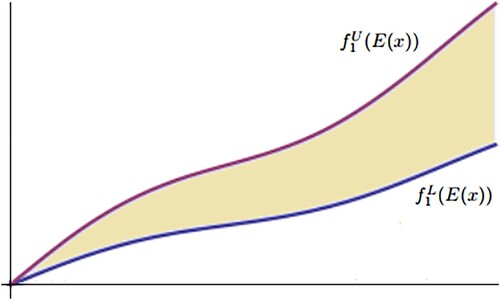
Figure 4. Graphical view of $f_2(E(x))$ of the problem (IVP1${}_E$).

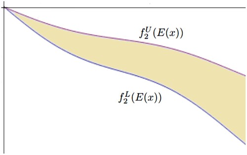
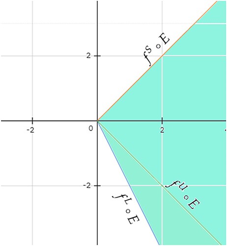
Figure 5. The set of all feasible solutions of (IVP1${}_E$).

4. Concluding remarks

In this paper, we have considered E-differentiable interval-valued vector optimization problems in which their optimal solutions are defined by LU and LS relations. The so-called E-Karush–Kuhn–Tucker necessary optimality conditions have been established for the considered E-differentiable interval-valued vector optimization problem for a weak LS-E-Pareto solution. Further, the sufficient optimality conditions for the so-called (weak) LU-E-Pareto and LS-E-Pareto optimality have been derived for the considered E-differentiable vector optimization problem with multiple interval-valued objective function under E-invexity and/or generalized E-invexity hypotheses. For the case of the (weak) LU-E-Pareto optimality, the results obtained here are more general than those ones obtained previously by Antczak and Abdulaleem [5]. This result has been illustrated in the paper by the suitable example of E-differentiable interval-valued vector optimization problem with E-differentiable E-invex function which is not an E-differentiable E-convex interval-valued function. For the (weak) LS-E-Pareto optimality, the results we obtained are novel for the class of E-differentiable vector optimization problems.

However, some interesting topics for further research remain. It would be of interest to investigate whether it is possible to prove similar optimality results for other classes of interval-valued optimization problems. We shall investigate these questions in subsequent papers.

Disclosure statement

No potential conflict of interest was reported by the author(s).

References

- N. Abdulaleem, E-optimality conditions for E-differentiable E-invex multiobjective programming problems, WSEAS Trans. Math. 18 (2019), pp. 14–27.
- N. Abdulaleem, E-invexity and generalized E-invexity in E-differentiable multiobjective programming, in ITM Web of Conferences, 2019, 24, 01002, pp. 1–12.
- N. Abdulaleem, Optimality and duality for E-differentiable multiobjective programming problems involving E-type I functions, J. Ind. Manag. Optim. 19(2) (2022), pp. 1513–1527.
- T. Antczak and N. Abdulaleem, E-optimality conditions and Wolfe E-duality for E-differentiable vector optimization problems with inequality and equality constraints, J. Nonlinear Sci. Appl. 12 (2019), pp. 745–764.
- T. Antczak and N. Abdulaleem, Optimality conditions for E-differentiable vector optimization problems with the multiple interval-valued objective function, J. Ind. Manag. Optim. 16 (2020), pp. 2971–2989.
- A.K. Bhurjee and G. Panda, Efficient solution of interval optimization problem, Math. Methods Oper. Res. 76 (2012), pp. 273–288.
- A.K. Bhurjee and S.K. Padhan, Optimality conditions and duality results for nondifferentiable interval optimization problems, J. Appl. Math. Comput. 50 (2016), pp. 59–71.
- Y. Chalco-Cano, W.A. Lodwick, and A. Rufián-Lizana, Optimality conditions of type KKT for optimization problem with interval-valued objective function via generalized derivative, Fuzzy Optim. Decis. Mak. 12 (2013), pp. 305–322.
- S. Chanas and D. Kuchta, Multiobjective programming in optimization of interval objective functions—A generalized approach, Eur. J. Oper. Res. 94 (1996), pp. 594–598.
- E. Hosseinzade and H. Hassanpour, The Karush–Kuhn–Tucker optimality conditions in interval-valued multiobjective programming problems, J. Appl. Math. Inform. 29 (2011), pp. 1157–1165.
- H. Ishibuchi and H. Tanaka, Multiobjective programming in optimization of the interval objective function, Eur. J. Oper. Res. 48 (1990), pp. 219–225.
- A. Jayswal, I. Stancu-Minasian, and I. Ahmad, On sufficiency and duality for a class of interval-valued programming problems, Appl. Math. Comput. 218 (2011), pp. 4119–4127.
- A. Jayswal, I. Stancu-Minasian, and J. Banerjee, Optimality conditions and duality for interval-valued optimization problems using convexifactors, Rend. Circ. Mat. Palermo. 65 (2016), pp. 17–32.
- A. Jayswal, I. Stancu-Minasian, J. Banerjee, and A.M. Stancu, Sufficiency and duality for optimization problems involving interval-valued invex functions in parametric form, Oper. Res. 15(1) (2015), pp. 137–161.
- A. Jayswal, I. Stancu-Minasian, and J. Banerjee, On interval-valued programming problem with invex functions, J. Nonlinear Convex Anal. 17(3) (2016), pp. 549–567.
- M. Jana and G. Panda, Solution of nonlinear interval vector optimization problem, Oper. Res. 14 (2014), pp. 71–85.
- S. Jha, P. Das, and S. Bandhyopadhyay, Characterization of LU-efficiency and saddle-point criteria for F-approximated multiobjective interval-valued variational problems, Results Cont. Optim. 4 (2021), pp. 100044, 1–11.
- S. Karmakar and A.K. Bhunia, An alternative optimization technique for interval objective constrained optimization problems via multiobjective programming, J. Egypt. Math. Soc. 22 (2014), pp. 292–303.
- V.I. Levin, Nonlinear optimization under interval uncertainty, Cybernet. Syst. Anal. 35 (1999), pp. 297–306.
- L. Li, S. Liu, and J. Zhang, On interval-valued invex mappings and optimality conditions for interval-valued optimization problems, J. Inequal. Appl. 179 (2015), pp. 1–19.
- J. Lin, Maximal vectors and multi-objective optimization, J. Optim. Theory Appl. 18 (1976), pp. 41–64.
- O.L. Mangasarian, Nonlinear Programming, McGraw-Hill Book Company, New York, 1969.
- A.E.M.A. Megahed, H.G. Gomma, E.A. Youness, and A.Z.H. El-Banna, Optimality conditions of E-convex programming for an E-differentiable function, J. Inequal. Appl. 246 (2013), pp. 1–11.
- R.E. Moore, Method and Applications of Interval Analysis, SIAM, Philadelphia, 1979.
- M.S. Rahman, A.A. Shaikh, and A.K. Bhunia, Necessary and sufficient optimality conditions for non-linear unconstrained and constrained optimization problem with interval valued objective function, Comput. Ind. Eng. 147 (2020), pp. 1–6.
- D. Singh, B.A. Dar, and A. Goyal, KKT optimality conditions for interval valued optimization problems, J. Nonlinear Anal. Optim. 5 (2014), pp. 91–103.
- D. Singh, B.A. Dar, and D.S. Kim, KKT optimality conditions in interval valued multi-objective programming with generalized differentiable functions, Eur. J. Oper. Res. 254 (2015), pp. 29–39.
- A.M. Stancu, Mathematical Programming with Type-I Functions, Matrix Rom, Bucharest.2013. p. 197.
- Y. Sun and L. Wang, Optimality conditions and duality in nondifferentiable interval-valued programming, J. Ind. Manag. Optim. 9 (2013), pp. 131–142.
- H-C. Wu, The Karush–Kuhn–Tucker optimality conditions in an optimization problem with interval-valued objective function, Eur. J. Oper. Res. 176 (2007), pp. 46–59.
- H-C. Wu, On interval-valued nonlinear programming problems, J. Math. Anal. Appl. 338 (2008), pp. 299–316.
- H-C. Wu, The Karush–Kuhn–Tucker optimality conditions in multiobjective programming problems with interval-valued objective functions, Eur. J. Oper. Res. 196 (2009), pp. 49–60.
- H-C. Wu, Duality theory for optimization problems with interval-valued objective functions, J. Optim. Theory Appl. 144 (2010), pp. 615–628.
- E.A. Youness, E-convex sets, E-convex functions, and E-convex programming, J. Optim. Theory Appl. 102 (1999), pp. 439–450.
- J.K. Zhang, S.Y. Liu, L.F. Li, and Q.X. Feng, The KKT optimality conditions in a class of generalized convex optimization problems with an interval-valued objective function, Optim. Lett. 8 (2014), pp. 607–631.