Interactive smart battery storage for a PV and wind hybrid energy management control based on conservative power theory

ABSTRACT

This paper presents interactive smart battery-based storage (BBS) for wind generator (WG) and photovoltaic (PV) systems. The BBS is composed of an asymmetric cascaded H-bridge multilevel inverter (ACMI) with staircase modulation. The structure is parallel to the WG and PV systems, allowing the ACMI to have a reduction in power losses compared to the usual solution for storage connected at the DC-link of the converter for WG or PV systems. Moreover, the BBS is embedded with a decision algorithm running real-time energy costs, plus a battery state-of-charge manager and power quality capabilities, making the described system in this paper very interactive, smart and multifunctional. The paper describes how BBS interacts with the WG and PV and how its performance is improved. Experimental results are presented showing the efficacy of this BBS for renewable energy applications.

KEYWORDS:

• Storage
• wind energy
• solar energy
• asymmetric multilevel inverter

1. Introduction

The power delivery industry faces the continuous growth of electrical energy consumption. As society needs more improvements in technology and in social advancements, more electrical energy is needed. Therefore, new electrical power resources and new ways of integration to the transmission or distribution grid are required. Recently, renewable energy sources have been applied as a long-term and promising solution to such energy challenges. Currently, distributed generation (DG) systems, which are composed of both renewable and non-renewable energy micro-sources, have been integrated into the power system's distribution level (Bhende, Mishra, & Malla, 2011; Kroposki et al., 2006). DG has a smaller size compared to traditional power plants. Such power generation units associated with their energy management and demand side control techniques are normally called microgrids, and when such microgrids have a high degree of control, integration with the utility and users, and several functionalities, they are called smartgrids (Chakraborty, Weiss, & Simoes, 2007).

It is very important to design appropriate power electronics for integration of renewable energy sources to the grid. (Kroposki et al., 2006). DG systems such as wind, micro-turbine, IC engine or flywheel storage, generate AC output voltage usually with variable frequency. Therefore, these DGs need an AC–DC converter to surpass the input distortion and frequency variation effects before merging to an AC-compatible grid voltage. Likewise, for DG systems with DC output voltage (such as photovoltaic (PV), fuel cells or batteries), a DC–DC converter is typically needed to boost the DC voltage level to the appropriate DC level (Carnieletto, Brandao, Suryanarayanan, Farret, & Simoes, 2010; Lute, Simoes, Brandao, Durra, & Muyeen, 2014). In both cases, once an appropriate DC voltage is achieved from converters, a grid-connected inverter (GCI) module is used in order to convert the primed DC voltage to grid-compatible AC power (Harirchi, Simões, Al-Durra, & Muyeen, 2015; Harirchi, Simões, Babakmehr, Al-Durra, & Muyeen, 2015). Finally, an output filtering module filters the AC output of the inverter (Reznik, Simões, Al-Durra, & Muyeen, 2014).

The most promising renewable sources are wind and solar energy. Both of them may operate in grid-tied or stand-alone conditions. Wind stand-alone systems are used to supply isolated loads requiring energy storage to manage the variable load demand. For such systems, the control scheme is designed to perform the management of power during fluctuation of wind and load demand (Barote, Marinescu, & Cirstea, 2013; Bhende, Mishra, & Malla, 2011; Lagorse, Simoes, & Miraoui, 2009). Power electronic inverters are used to control active/reactive power, frequency, and support grid voltage during faults (Angela, Liserre, Mastromauro, & Aquila, 2013; Li, Haskew, Swatloski, & Gathings, 2012).

Storage systems are very important in order to support PV and WG integration, since wind and solar energy may not fully satisfy the instantaneous power balance. There are several configurations to store energy, such as batteries, compressed air, flywheel, supercapacitor and pumped hydro. They have different power density, volume and time response. So, the way the energy is stored depends on the application. There are also differences between power and energy storage concepts. Storage for power applications is designed to supply power for a long timescale (hours). Pumped hydro and batteries are examples of power storage suited for bulky systems (Chakraborty, Simões, & Kramer, 2013). On the other hand, storage for energy applications is demanded when there is a need for a high time response. Supercapacitors may supply a great amount of energy in a short time complementing power quality (PQ) requirements, and slower storage systems are not capable of having a comparable performance.

Battery-based storage (BBS) combined to wind WG and PV is commonly found in real-world applications. The literature demonstrates the efficacy of using BBS to support the wind generator system (WGS) random nature (Barote, Marinescu, & Cirstea, 2013; Bhuiyan & Yazdani, 2009; Li, Joos, & Belanger, 2010). A BBS with WGS for a single-phase stand-alone structure is described by Li et al. (2010) and Bhuiyan and Yazdani (2009) and they present another stand-alone system containing a WG, a hydro generator and a BBS. The goals are mainly to achieve the maximum power-tracking and to control the magnitude and frequency of the output voltage. A multimode control for WG aggregated to a BBS unit for remote applications is presented by Barote, Marinescu, and Cirstea (2013).

This paper presents an alternative way of connecting the BBS with the WG and PV. Most of the past work described in the literature has a BBS connected parallel to the DC-link which interfaces the generator to the grid or loads. The proposed structure of this paper is to connect the BBS in parallel to the whole system by using a DC–AC converter. In this paper the authors propose the use of asymmetric cascade multilevel inverter topology with staircase modulation. Three battery banks are used with different capacities for those batteries.

The use of the multilevel inverter guarantees a reduction in power losses compared to the conventional structure. In storage systems, any reduction in power losses supports an increase in the time between charging cycles, with an overall improvement of storage response time. Moreover, the point of connection allows the BBS to perform ancillary services independent of the PV and WG system.

The asymmetric cascaded H-bridge multilevel inverter (ACMI) embedded with the staircase modulation allows the operation of the upper cell, which transfers the major part of the battery power, to be switched to 60 Hz. This low switching frequency contributes to the reduction of the power losses. Moreover, the ACMI allows a minimisation in the output filter volume due to the reduced voltage total harmonic distortion (THD) in the output voltage. The control strategy is based on the conservative power theory (CPT) (Busarello & Pomilio, 2015).

2. The battery storage system

Figure 1 presents a simplified unifilar (single-line) diagram of the proposed three-phase structure, where a grid with 127 Vrms and frequency of 60 Hz has been used. The BBS is connected in parallel to the WG and PV system. The ACMI is composed of three series-connected H-bridge modules with a voltage scaled 1:2:6, presenting 19 levels at its terminal voltage. The storage is divided in three banks, one for each module. The upper module has twelve 12 V lead acid batteries connected in a series. Similarly, the middle and lower modules have four and two 12 V lead acid batteries, respectively. The banks are connected at each DC side of the H-bridge module. The WG system is composed of a permanent magnet synchronous generator (PMSG), and it is connected to the grid through a back-to-back system. The PV system is composed of a solar array, an interleaved boost converter, plus one H-bridge converter. A nonlinear load, in this analysis made by a diode rectifier with an LC filter at the DC side, is connected to the PCC (point of common coupling).

Figure 1. Simplified diagram of the proposed three-phase structure.

2.1 The control strategy

Figure 2 shows the control strategy applied to the BBS. At the PCC voltage, the WG system output, the PV system output and the load current are individually measured and sent to the CPT real-time calculation module. The CPT calculation gives the current reference to be used in the BBS. A phase-locked loop (PLL) (Chung, 2000) supplies information about the PCC voltage phase angle. Once the current reference is defined, it is compared to the BBS output measured current, and the control signal is sent to the current controller. The current controller is a proportional-integrator (PI) with PCC voltage feedforward. The AMCI switch commands are modulated by staircase modulation. A decision algorithm based on the price of energy, on the state-of-charge (SOC) curve and on the power requirement decides the operation mode of the BBS.

Figure 2. Control strategy applied to the BBS.

2.2 The staircase modulation

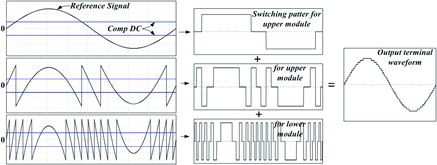
The possibility of the upper module switching to 60 Hz is due to the staircase modulation, also known as nearest level modulation (Perez, Rodriguez, Pontt, & Kouro, 2007). Figure 3 presents the principle of it. The reference is sinusoidal, and the pattern for each ACMI module is different. The reference for the upper module is obtained by comparing the reference to the DC value. Its result is the switching pattern for the upper module. The reference for the middle module is obtained by subtracting the sinusoidal reference from the switching pattern for the upper module. The resulting signal is then compared to another DC value. This process continues for the next module. Noticeably, the upper cell switches to 60 Hz. Moreover, the resulting output signal is close to the reference signal, indicating the possibility of a reduction in the volume of the output filter. The staircase modulation has the disadvantage of presenting a regenerative process in the smaller voltage cells depending on the fundamental component amplitude and it must be avoided (Rech & Pinheiro, 2007).

Figure 3. Principle of operation of the staircase modulation.

The reduction in power losses proposed in this paper may be verified. The switching losses are directly proportional to the voltage and current across a switch and also across the switching frequency. Figure 4 illustrates the voltage and current across a switch during a turn-on transition. The power losses (P_sw) are shown by the dashed area. The result is the higher the switching frequency, the higher the number of transitions and the higher the power losses. In a conventional pulse width modulation (PWM) converter with 10 kHz switching frequency, the number of commutations in a 60 Hz grid-cycle is around 300.

Figure 4. Voltage and current across a switch during a turn-on transition.

Regarding Figure 3, the voltage across the upper module has a 120 Hz frequency waveform. Therefore, the upper module transistors present four voltage and current transitions in a 60 Hz grid-cycle and once the upper cell process approximates 80% of the power, the reduction in losses is evident.

2.3 Decision algorithm

Figure 5 presents the flow chart of the decision algorithm based on the following rules about how the lead acid battery SOC is evaluated. If the battery needs to be charged, then the price of the energy is evaluated. If its value is considered feasible, the BBS charges its batteries with the unit power factor. The process of charging the batteries is called mode 1. The threshold voltage to charge the banks is 11.4 V for each battery. If the batteries do not need to be charged, the price of the energy is evaluated. If the price of the energy is considered high, then the BBS sells energy to the grid at nominal power; otherwise, the BBS supplies power to compensate for the intermittent behaviour of the PV and WG systems together. The process of selling energy to the grid with the unit power factor is called mode 2, while compensating for renewable behaviours is called mode 3. When the BBS either injects energy into the grid or charges its batteries, a PQ requirement may be applied. In this work, the PQ requirement is simplified by the fact that the grid current must present THDi lower than 5%, but a more complex and evolving PQ index performance can also be implemented. Therefore, the BBS injects active power and charges its batteries and also operates as an active filter simultaneously. The process of injecting active power with PQ improvement is called mode 4, and the process of charging the batteries with PQ improvement is called mode 5. There is also a mode in which the BBS operates exclusively as a shunt active filter. This mode is performed when the battery is at one of the two threshold points, and the price of energy is high. This mode is called mode 6.

Figure 5. The flow chart of the decision algorithm.

2.4 Battery model

In order to design integrated battery-based power electronics, a very good battery behavioural model is required which may include several parameters like SOC, terminal voltage, cell temperature, internal pressure and so on. There are many battery models in the literature (Chen & Rincon-Mora, 2006; Gao, Liu, & Dougal, 2002; Jackey, Plett, & Klein, 2009; Li, Mazzola, Gafford, & Younan, 2012; Plett, 2004; Salameh, Casacca, & Lynch, 1992; Wang et al., 2011). So, choosing a more complex or a more simplified model depends on the application. In a typical battery model, the applied current is the input, and the terminal voltage is the output (Chen & Rincon-Mora, 2006; Gao, Liu, & Dougal, 2002). However, in this work it was necessary to reverse the input–output relationship of the current and voltage, because the modelling of the BBS requires a voltage source as the input while the system operates in current-mode control in respect to the power flow to the utility grid. As described in the previous section, the decision algorithm makes use of the SOC curve in order to prescribe the operation mode. Therefore, a third-order battery model is used because it can guarantee the correct operation of the BBS. Figure 6 presents a typical SOC curve, obtained through a simulation (Sato & Kawamura, 2002), with two threshold points. The threshold points are the ones used in our decision algorithm, and their locations on the SOC curve were chosen using the criterion of the spinning reserve (Chakraborty, Simões, & Kramer, 2013).

Figure 6. The SOC curve and the threshold points used in the decision algorithm.

Figure 7 presents the third-order model of a lead acid battery (Wang et al., 2011) in which E_m is the open-circuit voltage, R₁ is the overvoltage resistance, C₁ is the overvoltage capacitance, R₂ is the internal resistance, I_P(V_PN) is the parasitic current in function of PN voltage, mainly caused by self-discharge, and R₀ is the terminal resistance.

Figure 7. Third-order model of lead acid batteries.

The model may be divided into three parts: (1) the main branch, composed of E_m, R₁, R₂ and C₁; (2) the parasitic branch, composed of the block called I_P(V_PN); and (3) the terminal branch, composed of the R₀.

The battery extracted charge is given by (1). (1) $$Q_{\mathrm{extr}}\left(t\right)=Q_{\mathrm{extr}\_\mathrm{ini}}-{\int }_0^t{i}_m\left(\tau \right)d\tau$$(1) where $Q_{\mathrm{extr}\_\mathrm{ini}}$ is the charge computed previously.

The battery total capacity is given by (2(2) $$C\left(i,T_{\mathrm{emp}}\right)=\frac{k{C}_0}{1+\left(k-1\right){\left(\frac{i}{i_{\mathrm{nom}}}\right)}^{\delta }}{\left(1-\frac{T_{\mathrm{emp}}}{T_{\mathrm{empf}}}\right)}^{ϵ}$$(2) ). (2) $$C\left(i,T_{\mathrm{emp}}\right)=\frac{k{C}_0}{1+\left(k-1\right){\left(\frac{i}{i_{\mathrm{nom}}}\right)}^{\delta }}{\left(1-\frac{T_{\mathrm{emp}}}{T_{\mathrm{empf}}}\right)}^{ϵ}$$(2) where k is the multiplier gain, C₀ is the no-load capacity at 0 °C, T_emp is the electrolyte temperature in °C (f means final), δ, ϵ are constants and i_nom is the battery nominal current.

The SOC is given by (3(3) $$\mathrm{SOC}=1-\frac{Q_{\mathrm{extr}}}{C\left(i,T_{\mathrm{emp}}\right)}$$(3) ). (3) $$\mathrm{SOC}=1-\frac{Q_{\mathrm{extr}}}{C\left(i,T_{\mathrm{emp}}\right)}$$(3)

The depth of discharge (DOD) is given by (4(4) $$\mathrm{DOD}=1-\frac{Q_{\mathrm{extr}}}{C\left(i_{\mathrm{avg}},T_{\mathrm{emp}}\right)}$$(4) ). (4) $$\mathrm{DOD}=1-\frac{Q_{\mathrm{extr}}}{C\left(i_{\mathrm{avg}},T_{\mathrm{emp}}\right)}$$(4)

By using the previous equations, the battery model parameter can be determined.

The overvoltage resistance is given by (5(5) $$R_1=-k_{R1}ln\left(\mathrm{DOD}\right)$$(5) ). (5) $$R_1=-k_{R1}ln\left(\mathrm{DOD}\right)$$(5) where k_R1 is a constant.

The overvoltage capacitance is given by (6(6) $$C_1=\frac{{\tau }_1}{R_1}$$(6) ). (6) $$C_1=\frac{{\tau }_1}{R_1}$$(6) where τ₁ is main branch constant time.

The internal resistance is given by (7(7) $$R_2=k_2\frac{e^{\left(k_{21}\left(1-\mathrm{SOC}\right)\right)}}{1+e^{\left(k_{22}\frac{i}{i_{\mathrm{nom}}}\right)}}$$(7) ). (7) $$R_2=k_2\frac{e^{\left(k_{21}\left(1-\mathrm{SOC}\right)\right)}}{1+e^{\left(k_{22}\frac{i}{i_{\mathrm{nom}}}\right)}}$$(7)

The terminal resistance is given by (8(8) $$R_0=R_{00}\left[1+k_a\left(1-\mathrm{SOC}\right)\right]$$(8) ). (8) $$R_0=R_{00}\left[1+k_a\left(1-\mathrm{SOC}\right)\right]$$(8) where R₀₀ is the terminal resistance at SOC = 1.

The parasitic current is given by (9(9) $$\begin{array}{ccc}\hfill I_P\left(V_{\mathrm{PN}}\right)& =& V_{\mathrm{PN}}{k}_{pn}\exp [\frac{V_{\mathrm{PN}}/\left({\tau }_{pn}+1\right)}{k_p}\hfill \\ & & +k_3\left(1-\frac{T_{\mathrm{emp}}}{T_{\mathrm{empf}}}\right)]\hfill \end{array}$$(9) ). (9) $$\begin{array}{ccc}\hfill I_P\left(V_{\mathrm{PN}}\right)& =& V_{\mathrm{PN}}{k}_{pn}\exp [\frac{V_{\mathrm{PN}}/\left({\tau }_{pn}+1\right)}{k_p}\hfill \\ & & +k_3\left(1-\frac{T_{\mathrm{emp}}}{T_{\mathrm{empf}}}\right)]\hfill \end{array}$$(9) where τ_n is the constant time of the parasitic branch. The battery terminal voltage is given by (10(10) $$v_t=E_m+i_m{Z}_{\mathrm{eq}}+i{R}_o$$(10) ). (10) $$v_t=E_m+i_m{Z}_{\mathrm{eq}}+i{R}_o$$(10) where Z_eq is given by (11). (11) $$Z_{\mathrm{eq}}=\frac{R_1+R_2+s{R}_1{R}_2{C}_1}{s{R}_1{C}_1+1}$$(11) And the i_m and i are related as (12(12) $$I_P=i_m-i$$(12) ). (12) $$I_P=i_m-i$$(12)

Although a state-space formulation leading to a transfer function expansion for the battery system can be developed as indicated in Hafsaoui et al. (2010), the authors of this paper preferred the equation oriented model for a circuit-based simulation in PSIM.

The battery capacity is found by looking into the manufacturer's datasheet, and the constants k presented in the previous equations are not easy to determine, but they can be found through specific experimental tests; such procedure is beyond the scope of this paper (Mandal & Cox, 2010; Plett, 2007).

The battery model is used to understand how the battery behaves. Based on the behaviour, the design of the BBS takes into account the interested aspect. In this case, the SOC curve is used. During operation, the current point of the SOC curve is estimated in order to be used as input information for the decision-taker algorithm through Equations (1)(1) $$Q_{\mathrm{extr}}\left(t\right)=Q_{\mathrm{extr}\_\mathrm{ini}}-{\int }_0^t{i}_m\left(\tau \right)d\tau$$(1) –(3(3) $$\mathrm{SOC}=1-\frac{Q_{\mathrm{extr}}}{C\left(i,T_{\mathrm{emp}}\right)}$$(3) ).

2.1.4 BBS current reference

The methodology described here is presented for a single-phase grid, but it is extended to a three-phase grid, with or without four wires without any loss of generality. Each one of the six modes of operation has its current reference. The mode 1 BBS current reference is given by (13(13) $$i_{\mathrm{BBS}1}^{*}\left(t\right)=\frac{P_{\mathrm{charge}}}{V_{\mathrm{PCC}}}\sin \left(\omega t+\varphi -\pi \right)$$(13) ). (13) $$i_{\mathrm{BBS}1}^{*}\left(t\right)=\frac{P_{\mathrm{charge}}}{V_{\mathrm{PCC}}}\sin \left(\omega t+\varphi -\pi \right)$$(13) where ϕ is the PCC phase angle supplied by the PLL, and P_charge is the power reference to charge the batteries.

Similarly, the mode 2 BBS current reference is given by (14(14) $$i_{\mathrm{BBS}2}^{*}\left(t\right)=\frac{P_{\mathrm{nom}}}{V_{\mathrm{PCC}}}\sin \left(\omega t+\varphi \right)$$(14) ): (14) $$i_{\mathrm{BBS}2}^{*}\left(t\right)=\frac{P_{\mathrm{nom}}}{V_{\mathrm{PCC}}}\sin \left(\omega t+\varphi \right)$$(14) where P_nom is the nominal power of the storage. The mode 3 operates according to the difference between the nominal power of the storage and the WG and PV instantaneous output power. Therefore, the active power reference for the BBS is given by (15(15) $$P_{\mathrm{BBS}}^{*}\left(t\right)=1-P_{\mathrm{PV}}\left(t\right)-P_{\mathrm{WG}}\left(t\right)\left(\mathrm{pu}\right),$$(15) ): (15) $$P_{\mathrm{BBS}}^{*}\left(t\right)=1-P_{\mathrm{PV}}\left(t\right)-P_{\mathrm{WG}}\left(t\right)\left(\mathrm{pu}\right),$$(15) where P_WG and P_PV are the WG and PV system output power. The right side of (15(15) $$P_{\mathrm{BBS}}^{*}\left(t\right)=1-P_{\mathrm{PV}}\left(t\right)-P_{\mathrm{WG}}\left(t\right)\left(\mathrm{pu}\right),$$(15) ) has three parts. The first is a unit because the equation is written per unit (pu). The second and third are P_WG and P_PV, obtained by measurement.

The proposed BBS operates only with the active power. However, the WG and PV system may supply more than just active power, it might supply reactive power and also harmonic currents. Therefore, for this study the BBS must extract only the active power information from the WG and PV output power; that is how the CPT is used. The authors will investigate further uses of CPT for improved extra functionalities in the future.

According to the CPT, for a given voltage v(t) and a currenti(t), the active current for one phase is given by (16(16) $$i_{\mathrm{active}}\left(t\right)=\frac{\frac{1}{T}{\int }_t^{t+T}v\left(t\right)i\left(t\right)dt}{v_{\mathrm{rms}}}v\left(t\right)$$(16) ): (16) $$i_{\mathrm{active}}\left(t\right)=\frac{\frac{1}{T}{\int }_t^{t+T}v\left(t\right)i\left(t\right)dt}{v_{\mathrm{rms}}}v\left(t\right)$$(16)

Therefore, the WG output active current is given by (17(17) $$i_{\mathrm{WG}\_\mathrm{active}}\left(t\right)=\frac{\frac{1}{T}{\int }_t^{t+T}{v}_{\mathrm{PCC}}\left(t\right)i_{\mathrm{WG}}\left(t\right)dt}{V_{\mathrm{PCC}}}{v}_{\mathrm{PCC}}\left(t\right),$$(17) ): (17) $$i_{\mathrm{WG}\_\mathrm{active}}\left(t\right)=\frac{\frac{1}{T}{\int }_t^{t+T}{v}_{\mathrm{PCC}}\left(t\right)i_{\mathrm{WG}}\left(t\right)dt}{V_{\mathrm{PCC}}}{v}_{\mathrm{PCC}}\left(t\right),$$(17) where V_PCC is the root mean square (RMS) value of the PCC voltage. The WG system output active power is given by (18(18) $$P_{\mathrm{WG}}\left(t\right)=\frac{1}{T}{\int }_t^{t+T}{v}_{\mathrm{PCC}}\left(t\right)i_{\mathrm{WG}\_\mathrm{active}}\left(t\right)dt$$(18) ): (18) $$P_{\mathrm{WG}}\left(t\right)=\frac{1}{T}{\int }_t^{t+T}{v}_{\mathrm{PCC}}\left(t\right)i_{\mathrm{WG}\_\mathrm{active}}\left(t\right)dt$$(18)

Similarly, the output active current of the PV system is given by (19(19) $$i_{\mathrm{PV}\_\mathrm{active}}\left(t\right)=\frac{\frac{1}{T}{\int }_t^{t+T}{v}_{\mathrm{PCC}}\left(t\right)i_{\mathrm{PV}}\left(t\right)dt}{V_{\mathrm{PCC}}}{v}_{\mathrm{PCC}}\left(t\right)$$(19) ): (19) $$i_{\mathrm{PV}\_\mathrm{active}}\left(t\right)=\frac{\frac{1}{T}{\int }_t^{t+T}{v}_{\mathrm{PCC}}\left(t\right)i_{\mathrm{PV}}\left(t\right)dt}{V_{\mathrm{PCC}}}{v}_{\mathrm{PCC}}\left(t\right)$$(19)

And the output active power of the PV system is given by (20(20) $$P_{\mathrm{PV}}\left(t\right)=\frac{1}{T}{\int }_t^{t+T}{v}_{\mathrm{PCC}}\left(t\right)i_{\mathrm{PV}\_\mathrm{active}}\left(t\right)dt.$$(20) ): (20) $$P_{\mathrm{PV}}\left(t\right)=\frac{1}{T}{\int }_t^{t+T}{v}_{\mathrm{PCC}}\left(t\right)i_{\mathrm{PV}\_\mathrm{active}}\left(t\right)dt.$$(20)

The mode 3 BBS current reference is given by (21(21) $$i_{\mathrm{BBS}}^{*}\left(t\right)=\frac{P_{\mathrm{BBS}}^{*}}{V_{\mathrm{PCC}}}\sin \left(\omega t+\varphi \right).$$(21) ):(21) $$i_{\mathrm{BBS}}^{*}\left(t\right)=\frac{P_{\mathrm{BBS}}^{*}}{V_{\mathrm{PCC}}}\sin \left(\omega t+\varphi \right).$$(21)

The modes 4–6 deal with active filtering. Therefore, in order to obtain the current reference for these modes, the CPT is also used. The BBS active filter current reference is given by (22(22) $$i_{\mathrm{BBS}\_\mathrm{AF}}\left(t\right)=i_{\mathrm{load}}\left(t\right)-\frac{\frac{1}{T}{\int }_t^{t+T}v\left(t\right)i_{\mathrm{load}}\left(t\right)dt}{v_{\mathrm{rms}}}v\left(t\right)$$(22) ), which must be added to mode 4 and mode 5 references and used alone in mode 6 as a current reference. (22) $$i_{\mathrm{BBS}\_\mathrm{AF}}\left(t\right)=i_{\mathrm{load}}\left(t\right)-\frac{\frac{1}{T}{\int }_t^{t+T}v\left(t\right)i_{\mathrm{load}}\left(t\right)dt}{v_{\mathrm{rms}}}v\left(t\right)$$(22)

3. System implementation

The three-phase system presented in Figure 1 was simulated in PSIM. In order to make the simulation more realistic and to evaluate the system's dynamic behaviour, the BBS, the PV and the WG were simulated by using the switching converters. Therefore, a brief description on how the WG and PV systems were designed and simulated results are presented in the following section.

3.1 Wind generator system

This section describes the WG system (Li & Chen, 2008; Simoes, Bose, & Spiegel, 1997). The power transfer and control of a wind turbine system is based on PMSG and connected to the three-phase grid using a back-to-back converter. The machine side converter is controlled to extract the maximum power from wind using vector control. The grid side controller is designed to control the power flow using α–β reference frame. The power transfer strategy is proposed to control the flow of the power between the WT and the grid. Figure 8 presents the WG system and its control strategy. When the wind goes through the turbine, a mechanical torque (T_W) is applied to the PMSG. Measured wind speed (for example with anemometer) is used to get the optimum rotor speed required to achieve the maximum power from the wind turbine. The speed of the rotor is measured in order to compensate for the error of the controller and the reference of the direct axis current is zero. The PIs of the d-axis and q-axis can be designed using a small-signal (average) model, and the d–q reference voltages are transformed using Clarke and Park transformations to form three-phase reference voltages to command the switches of the converter using the sinusoidal pulse width modulation (SPWM) method. The DC-link voltage is controlled in a constant value by the grid side converter.

Figure 8. Wind turbine model and control scheme.

3.1.1 Wind turbine model

The air motion across the wind turbine produces mechanical power expressed as (23(23) $$P_w=\frac{1}{2}{C}_p\left(\lambda ,\beta \right)A_w{\rho }_{\mathrm{air}}{v}_W^3,$$(23) ). (23) $$P_w=\frac{1}{2}{C}_p\left(\lambda ,\beta \right)A_w{\rho }_{\mathrm{air}}{v}_W^3,$$(23) where the power coefficientC_p is a function of pitch angle and tip speed ratio is expressed as (24(24) $$C_p\left(\lambda ,\beta \right)=c_1\left(c_2\frac{1}{\gamma }-c_3\beta -c_4{\beta }^x-c_5\right)e^{-\frac{c_6}{\gamma }}$$(24) ) (Lubosny, 2003, pp. 80–81) (24) $$C_p\left(\lambda ,\beta \right)=c_1\left(c_2\frac{1}{\gamma }-c_3\beta -c_4{\beta }^x-c_5\right)e^{-\frac{c_6}{\gamma }}$$(24)

The coefficientsγ, x and c₁ − c₆ in (25(25) $$\begin{array}{ccc}& & c_1=0.5,c_2=116,c_3=0.4,c_4=0,c_5=5,\hfill \\ & & c_6=21,x=0,\hfill \end{array}$$(25) ) can be defined in different ways based on the type of turbine rotor (Erich & Renouard, 2013). The coefficients defined in Lubosny (2003) are used for the wind turbine model where (25) $$\begin{array}{ccc}& & c_1=0.5,c_2=116,c_3=0.4,c_4=0,c_5=5,\hfill \\ & & c_6=21,x=0,\hfill \end{array}$$(25) (26) $$\frac{1}{\gamma }=\frac{1}{\gamma +0.08*\beta }-\frac{0.035}{1+{\beta }^3}$$(26)

The tip speed ratio is defined as (27(27) $$\lambda =\frac{R_W{\omega }_r}{v_W},$$(27) ): (27) $$\lambda =\frac{R_W{\omega }_r}{v_W},$$(27) where R_W is the radius of the turbine's blades, ω_r is the turbine rotor speed and v_W is the average wind speed.

3.1.2 PSMG model

The d–q equivalent circuits of PMSG are described (Krishnan, 2010, pp. 226–260). The core loss is ignored in the circuits assuming high core resistance. The equations of the d-axis and q-axis in rotating reference frame are given as (28(28) $$v_{ds}^r=-R_s{i}_d-L_d\frac{d}{dt}{i}_d-{\omega }_e{L}_q{i}_q$$(28) ) and (29(29) $$v_{qs}^r=-R_{s}iq-L_q\frac{d}{dt}{i}_q+{\omega }_e{L}_d{i}_d+{\omega }_e{\psi }_m$$(29) ). (28) $$v_{ds}^r=-R_s{i}_d-L_d\frac{d}{dt}{i}_d-{\omega }_e{L}_q{i}_q$$(28) (29) $$v_{qs}^r=-R_{s}iq-L_q\frac{d}{dt}{i}_q+{\omega }_e{L}_d{i}_d+{\omega }_e{\psi }_m$$(29)

The instantaneous power is given by (30(30) $$P_i=\frac{2}{3}\left[v_{ds}^r{i}_d+v_{qs}^r{i}_q\right]$$(30) ): (30) $$P_i=\frac{2}{3}\left[v_{ds}^r{i}_d+v_{qs}^r{i}_q\right]$$(30)

Replacing (28(28) $$v_{ds}^r=-R_s{i}_d-L_d\frac{d}{dt}{i}_d-{\omega }_e{L}_q{i}_q$$(28) ) and (29(29) $$v_{qs}^r=-R_{s}iq-L_q\frac{d}{dt}{i}_q+{\omega }_e{L}_d{i}_d+{\omega }_e{\psi }_m$$(29) ) in the power equation and from the air gap power, the electromagnetic torque is given by (31(31) $$T_e=\frac{3}{4}p\left[{\psi }_m+\left(L_d-L-q\right)i_d\right]i_q$$(31) ): (31) $$T_e=\frac{3}{4}p\left[{\psi }_m+\left(L_d-L-q\right)i_d\right]i_q$$(31)

Then, the rotational angular speed is expressed as (32(32) $$\frac{d}{dt}{\omega }_r=\frac{1}{J}\left(T_W-T_e-B{\omega }_r\right),$$(32) ):(32) $$\frac{d}{dt}{\omega }_r=\frac{1}{J}\left(T_W-T_e-B{\omega }_r\right),$$(32) where T_W is the torque produced by the wind turbine, and T_e is the turbine equivalent moment of inertia, and B is the friction coefficient. The angular electrical speed is related to the rotor speed by (33(33) $${\omega }_e=\frac{p}{2}{\omega }_r,$$(33) ). (33) $${\omega }_e=\frac{p}{2}{\omega }_r,$$(33) where p is the number of poles of the synchronous machine.

3.1.3 Machine side controller

The purpose of the machine side controller is to track the optimum point of the rotor and extract the maximum power existing in the turbine. For a given wind turbine, the maximum power occurs at the maximum power coefficient (C_{p, max}) of the turbine. For a given wind speed, there is an optimum rotor speed that gives the optimum tip speed ratio (34(34) $${\lambda }_{\mathrm{opt}}=\frac{R_W{\omega }_{r,\mathrm{opt}}}{v_W}$$(34) ): (34) $${\lambda }_{\mathrm{opt}}=\frac{R_W{\omega }_{r,\mathrm{opt}}}{v_W}$$(34)

A simple approach to extract the maximum power is to calculate the optimum tip speed ratio ahead of time and then calculate the required rotor speed for any measured wind speed as (35(35) $${\omega }_{r,\mathrm{opt}}=\frac{v_W{\lambda }_{\mathrm{opt}}}{R_W}$$(35) ). (35) $${\omega }_{r,\mathrm{opt}}=\frac{v_W{\lambda }_{\mathrm{opt}}}{R_W}$$(35)

The maximum power, though, occurs at the optimum speed for every wind speed (v_W). As the wind speed changes from one point to another, the optimum point changes to a different value. A controller must be designed to follow the reference speed, and different techniques can be applied using a search technique that does not need measurement of the wind speed or use the direct relationship as in (35(35) $${\omega }_{r,\mathrm{opt}}=\frac{v_W{\lambda }_{\mathrm{opt}}}{R_W}$$(35) ).

3.1.4 Grid side controller

The purpose of the grid side converter is to inject electrical power in the grid produced by the generator with a good PQ. Moreover, the DC-link voltage control is also commanded by the grid side converter. The converter output current flows through the grid. Therefore, it is desirable that this current has a sinusoidal waveform. Figure 9 presents the α-axis control loop used in the grid side converter, and a similar closed loop is used for the β-axis. The grid converter output current is controlled by the inner loop and has a faster response than the DC-link loop. Therefore, the inner loop is considered unitary when the DC-link voltage control is designed. The power calculation uses the active and reactive power references to produce the current references, which in turn will be multiplied by the DC-link controller output signal. Then the signal is used to command the inverter.

Figure 9. α-axis control loop.

The PWM block could be assumed to have a gain of one. The power calculation block is given by (36(36) $$i_{\alpha ,\mathrm{power}}\left(s\right)=\frac{2}{3}\frac{v_{s\alpha }}{v_{s\alpha }^2+v_{s\beta }^2}{P}_{\mathrm{ref}}\left(s\right)+\frac{2}{3}\frac{v_{s\beta }}{v_{s\alpha }^2+v_{s\beta }^2}{Q}_{\mathrm{ref}}\left(s\right).$$(36) ) (Yazdani & Iravani, 2010, pp. 163–164) (36) $$i_{\alpha ,\mathrm{power}}\left(s\right)=\frac{2}{3}\frac{v_{s\alpha }}{v_{s\alpha }^2+v_{s\beta }^2}{P}_{\mathrm{ref}}\left(s\right)+\frac{2}{3}\frac{v_{s\beta }}{v_{s\alpha }^2+v_{s\beta }^2}{Q}_{\mathrm{ref}}\left(s\right).$$(36)

The inverter plus the filter connecting the inverter to the grid can be expressed as (37(37) $$\mathrm{IF}\left(s\right)=\frac{V_{\mathrm{DC}}/\phantom{V_{\mathrm{DC}}2}2}{}$$(37) ). (37) $$\mathrm{IF}\left(s\right)=\frac{V_{\mathrm{DC}}/\phantom{V_{\mathrm{DC}}2}2}{}$$(37)

The DC-link plant is given by (38(38) $$V_{\mathrm{D}{\mathrm{C}}_{\mathrm{link}}}\left(s\right)=\frac{2}{s{C}_{\mathrm{DC}}{V}_{s,pk}}.$$(38) ): (38) $$V_{\mathrm{D}{\mathrm{C}}_{\mathrm{link}}}\left(s\right)=\frac{2}{s{C}_{\mathrm{DC}}{V}_{s,pk}}.$$(38)

The current controller is composed of a phase-lead and phase-lag controller and the voltage control is a PI. Both are designed using classical frequency-response techniques. The designed controller transfer functions for the current and voltage are given by (39(39) $$C_i\left(s\right)=\frac{s2.804233·{10}^{-4}+1}{s^{2}3.840346·{10}^{-11}+s1.377492·{10}^{-6}},$$(39) ) and (40(40) $$C_{v_{\mathrm{DC}}}\left(s\right)=0.232\frac{s+0.03}{s}$$(40) ). (39) $$C_i\left(s\right)=\frac{s2.804233·{10}^{-4}+1}{s^{2}3.840346·{10}^{-11}+s1.377492·{10}^{-6}},$$(39) (40) $$C_{v_{\mathrm{DC}}}\left(s\right)=0.232\frac{s+0.03}{s}$$(40)

Figures 10 and 11 present the Bode diagrams for the current loop and for the voltage loop, respectively.

Figure 10. Bode diagram for the current loop.

Figure 11. Bode diagram for the voltage loop.

The PMSG parameters are similar and presented in Table 1 (Xia, Ahmed, & Williams, 2011). The wind turbine has the optimum wind speed of 200 rpm at 10 m/s rated wind speed.

Table 1. PMSG parameters and wind turbine specifications.

PMSG
Rs (stator resistance)	0.672 Ω
Ld (d-axis leakage inductance)	13.47 mH
Lq (q-axis leakage inductance)	13.47 mH
ψm (leakage inductance)	2.39 Wb
P (number of poles of machines)	24
Wind turbine
Nominal output power	10 kW
Base wind speed	10 m/s
Base rotor speed	200 rpm

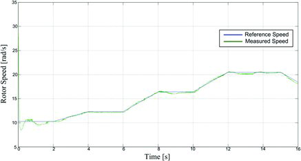
The performance of the machine and grid side converter is evaluated. The wind turbine tracks the maximum power point (MPP) as shown in Figure 12. The DC-link voltage is kept constant at 1400 V by the grid side converter.

Figure 12. Measured (red) and reference (blue) rotor speed in rad/s.

Figure 13 presents the DC-link voltage in steady-state condition. It is constant and controlled at 1400 V.

Figure 13. DC-link voltage in steady-state condition.

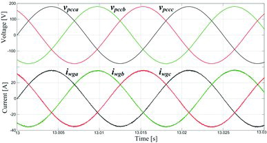
Figure 14 presents the three-phase PCC voltage and the WG three-phase output current in a steady-state condition. The current is sinusoidal and in phase with the PCC voltage.

Figure 14. The three-phase PCC voltage and the WG three-phase output current in steady-state condition.

3.2 PV system

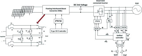
This section describes the PV system designed. The schematic of the proposed power electronic interface for a grid-connected PV-based system and its control strategy is shown in Figure 15. A floating four-leg interleaved boost converter (FIBC) and a smart grid-connected inverter (SGCI) were used. The FIBCs for PV and fuel cell applications are used because of their high voltage gain, high efficiency, low input current ripple and smaller components (capacitors and inductors) (Lute et al., 2014). In this paper, a type-III compensator is designed in order to control the output voltage of the FIBC and support a high gain and constant DC-link voltage for the SGCI in the full FIBC–SGCI interface. In order to limit the effect of the harmonics, the SGCI is connected to the grid through an LCL filter module. The proposed control technique for the SGCI is based on d − q theory, where a smooth transition method is applied in order to switch between GC and islanding modes.

Figure 15. Schematic of the proposed power electronic interface for grid-connected PV-based system and its control strategy.

3.2.1 Designing a controller for FIBC

A controller for DC–DC FIBC with an input voltage of 25 V (which is the output voltage of PV modules) and an output voltage of 380 V is presented in this section. A type-III controller is selected to control this converter, and the controller contains a closed-loop error amplifier circuit, a power stage and a PWM unit. The PWM has been used in order to apply the output control signal from the compensator to the FIBC switches. The error amplifier compares the converter output voltage with a reference voltage in order to produce an error signal that is used to adjust the duty ratio of the switch. The small-signal transfer function of the type-III amplifier is expressed in terms of its input and feedback impedances Z_i and Z_f and given by (41(41) $$G\left(s\right)=\frac{V_c\left(s\right)}{V_o\left(s\right)}=-\frac{Z_f}{Z_i}=-\frac{\left(R_2+\frac{1}{s{C}_1}\right)\parallel \frac{1}{s{C}_2}}{R_1\parallel \left(R_3+\frac{1}{s{C}_3}\right)}$$(41) ): (41) $$G\left(s\right)=\frac{V_c\left(s\right)}{V_o\left(s\right)}=-\frac{Z_f}{Z_i}=-\frac{\left(R_2+\frac{1}{s{C}_1}\right)\parallel \frac{1}{s{C}_2}}{R_1\parallel \left(R_3+\frac{1}{s{C}_3}\right)}$$(41)

There are two well-known methods for designing a type III error amplifier. The first method is the K factor method (Fernandez et al., 2013); the second method (Raut & Talukder, 2011) is called manual placement of poles and zeros (MPPZ). In the MPPZ approach, the resonant frequency of the LC filter is used and given by (42(42) $$f_{\mathrm{LC}}=\frac{1}{2\pi \sqrt{\mathrm{LC}}}$$(42) ). (42) $$f_{\mathrm{LC}}=\frac{1}{2\pi \sqrt{\mathrm{LC}}}$$(42)

The first zero is commonly placed at 50%–100% of thef_LC, while the second zero is placed at f_LC. The second pole is placed at the equivalent series resistance (ESR) zero in the filter transfer function (1/(r_cc)); the third pole is placed at one-half of the switching frequency. The values for the controller zeros and poles are as follows: ω_z1= 461.2667, ω_z2= 922.5334, ω_p1= 0, ω_p2= 5.1894k and ω_p3= 62.832k. Table 2 represents the parameters of the designated compensators.

Table 2. Parameters of the type-III compensator.

C1 = 0.2 nF	R1 = 1 kΩ
C2 = 1.5 nF	R2 = 120 kΩ
C3 = 1 uF	R3 = 15 Ω

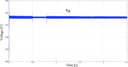
Figure 16 presents the FIBC output voltage in steady-state condition when the PV system is injecting 2 kW into the grid. It is verified that the FIBC output voltage is controlled at 380 V.

Figure 16. The FIBC output voltage in steady-state condition when the PV system is injecting 2 kW into the grid.

3.2.2 Smart grid-connected inverter (SGCI)

Controlling the injected power is the most important issue during the grid-connected mode (Hu, Kuo, Lee, & Guerrero, 2011). In order to achieve this goal, the current components are controlled. Due to the DC nature of the d − q components in the d–q reference frame, a PI controller is used to control the d and q components of currents. Moreover, since the d and q control loops have the same dynamics, the tuning of the PI controller for the current is done only for the d-axis.

The reference values of currents are calculated from (43(43) $$P_{\mathrm{ref}}=\frac{3}{2}\left(V_d{I_d}^{*}+V_q{I_q}^{*}\right)$$(43) ) and (44(44) $$Q_{\mathrm{ref}}=\frac{3}{2}\left(V_q{I_d}^{*}-V_d{I_q}^{*}\right)$$(44) ), where P_ref and Q_ref are determined, for example, by an energy management system in addition to power negotiation with the main grid. (43) $$P_{\mathrm{ref}}=\frac{3}{2}\left(V_d{I_d}^{*}+V_q{I_q}^{*}\right)$$(43) (44) $$Q_{\mathrm{ref}}=\frac{3}{2}\left(V_q{I_d}^{*}-V_d{I_q}^{*}\right)$$(44)

Table 3 presents the FIBC parameters, while in Table 4 the SGCI is presented. For this set of simulations, the reference values for active and reactive powers are set to 2 kW and 0 kVAR, respectively.

Table 3. Parameters of FIBC.

Input voltage	Vin = 25 V
Output voltage	Vout = 380 V
Inductor	L = 250e-6 H
Capacitor	C = 4.7e-3 F
Duty cycle	D = 0.876
Output capacitor ESR	r = 41e-3 Ω
Switching frequency	20 kHz

Table 4. Parameters of the inverter.

Input voltage	VDC= 380 V
Output voltage (1Ф)	Vout = 120 Vrms
Inductor of LCL	L = 1e-3 H
Capacitor of LCL	C = 0.1e-6 F
Switching frequency	Fsw = 15 KHz
Frequency of the grid	fg = 60 Hz

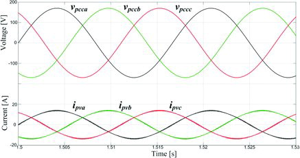
Figure 17 presents the three-phase PCC voltage and the three-phase PV system output current. Similar to the WG system, the current is sinusoidal and in phase with the PCC voltage.

Figure 17. The three-phase PCC voltage and the three-phase PV system output current in steady-state condition.

3.3 The whole system

The three-phase system presented in Figure 1 was simulated. The parameters are presented in Table 5. The batteries were simulated by using the battery model found in the PSIM software.

Table 5. Prototype parameters.

RMS phase-voltage grid	Vgrid = 127 V
Grid frequency	fgrid = 60 Hz
BBS output inductance	LBBS = 4.25 mH
Inverter upper module voltage	Vh = 144 V (12 × 12 V battery)
Inverter middle module voltage	Vm = 48 V (4 × 12 V battery)
Inverter lower module voltage	VL = 24 V (2 × 12 V battery)

Figure 18 presents the PV, the WG and the BBS output power, as well as the sum of them for phase A. The PV and the WG supply a variable power due to the intermittent behaviour found in renewable sources. At t = 1.5 s, the BBS begins to operate. It is noticeable that the BBS compensates for the deficiency of the PV and WG systems. Consequently, the grid receives constant power independently of wind and sun conditions. During the interval between 3.2 and 4.9 s, the PV and WG both supply nominal power. Therefore, the BBS does not inject any power, and the BBS will charge its battery bank.

Figure 18. The PV, the WG and the BBS output power, as well as the sum of them for phase A.

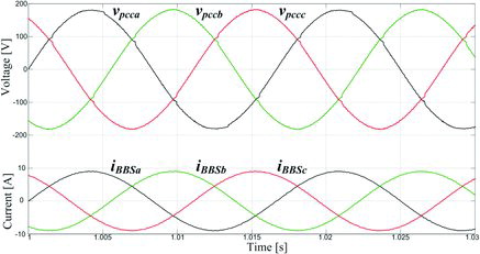
Figure 19 presents the three-phase PCC voltage and the three-phase BBS output current under mode 2. The BBS output current is sinusoidal and in phase with the PCC voltage.

Figure 19. Three-phase PCC voltage and the three-phase BBS output current in steady-state condition under mode 2.

Figure 20 presents the BBS terminal voltage for each module for phase A. The upper waveform is the upper module terminal voltage. As previously described, the number of commutations is reduced, indicating a reduction in the power losses.

Figure 20. BBS terminal voltage for each module for phase A.

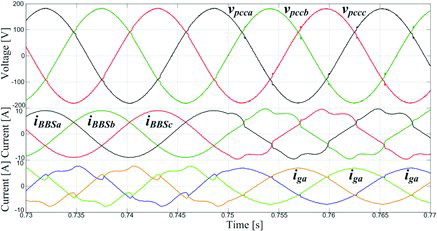
Figure 21 presents the PCC voltage, the BBS current and the grid current during the transition from mode 2 to mode 4. During this transition, the BBS begins to operate as an active filter in addition to providing injection power. Before t = 0.75 s, the BBS injects active power with unity power factor. Its output current is sinusoidal and in phase with the PCC voltage. Once there is a nonlinear load connected to the PCC and there is no filter to compensate the harmonic currents, the grid current is distorted. At t = 0.75 s, the BBS begins to operate as an active filter simultaneously with the injection power mode. As a result, its output current is distorted because of the harmonic currents and the grid current becomes sinusoidal. Now, one of the smart features of the proposed BBS appears. The grid begins absorbing active power injected by PV, the WG and BBS, as can be observed in the same figure by the 180° displacement between the PCC voltage and the grid current. Even absorbing active power, the grid is receiving active filter compensation by means of the BBS.

Figure 21. The PCC voltage, the BBS current and the grid current when the BBS during the transition from mode 2 to mode 4.

4. Experimental results

The system presented in Figure 1 has been partially verified experimentally with a single-phase 2 kVA prototype. The experiment uses the same parameters as in simulation. Although the experimental set-up could not have a full WG and PV because of laboratory resource limitations, the BBS system was embedded with a fictitious WG and PV output power curve behaviour. Such a curve emulates the information produced from the WG and PV systems, and the curve demonstrates similar currents. As can be observed, the experimental results demonstrate the efficacy of the BBS. The control strategy and the decision algorithm were embedded in the float-point digital signal controller TMS320L28335. The experimental results presented in this section come from the flow chart presented in Figure 3. The measured variables are referred to those presented in Figure 1.

Figure 22 presents the PCC voltage, BBS output current and the load current during transition from mode 2 to mode 1. Initially, the price of the energy is the one expected, and the BBS output current is sinusoidal and in phase related to the PCC voltage, which means that the BBS injects active power into the grid. Later, the BBS begins to charge the batteries with the unity power factor from the grid's point of view. As a result, the BBS output current is 180° phase-shift related to the PCC voltage. The load current is kept unchanged.

Figure 22. PCC voltage, BBS output current and the load current during transition from mode 2 to mode 1.

Figure 23 presents the BBS terminal voltage and the cell output voltages during mode 2 in a steady-state condition. The terminal voltage has 19 levels, and it produces a sinusoidal waveform with a reduced output filter. The upper cell output voltage is a quasi-square waveform with 60 Hz frequency. Since the commutation number in this module is reduced, it is expected that a reduction in the switching losses will be observed compared to other topologies.

Figure 23. The BBS terminal voltage (v_t) and the cell output voltages (v_{t_h}, v_{t_m} and v_{t_L}) (R1, R2, R3, Ch4: 500 mV/250 V).

Figure 24 presents the BBS output current measured on a long timescale and a detail of a short timescale when the WG and PV systems are emulated. This operation corresponds to mode 3 as previously explained. The BBS output current amplitude changes because it is injecting power according to the difference between the WG and PV instantaneous output power. Therefore, the sum of the BBS and WG and the PV output powers is constant. The figure shows that the BBS output current is sinusoidal.

Figure 24. The BBS output current measured in a long timescale and a detail of a short period when the WG and PV systems are emulated, mode 3 (Ch1: 0.1 V/A).

Figure 25 shows the PCC voltage, the BBS, the grid and load currents when the BBS operates exclusively as an active filter (mode 6). The BBS output current is highly distorted and the achieved grid current waveform is close to the PCC voltage. This is because the CPT forces the grid current to follow the PCC waveform, similar to resistive load behaviour.

Figure 25. PCC voltage, the BBS, the grid and load currents when the BBS is operating exclusively as active filter (mode 6).

5. Conclusions

Connecting a storage system in parallel to both WG and PV systems is an effective solution for supplying constant power to a system with a nonlinear load. Besides the main functions of the proposed smart battery-based system, the required active power is supplied with a sinusoidal current waveform using CPT. The implemented asymmetric cascaded multilevel inverter shows the advantage of transferring the major part of the power under 60 Hz switching frequency. Consequently, the commutation number is reduced and the power losses are minimised as shown in both simulation and experimental results. Moreover, the dimensioning of the output filter is reduced. Experimental results show a very efficient performance of the BBS. Neither unpredictability nor instability was observed. The proposed full-fledged system described in this paper is a potential candidate towards a novel solution of a hybrid storage system associated with WG and PV systems. The simulation file used in this paper will be freely available on https://sites.google.com/site/busarellosmartgrid/home.

Acknowledgements

The authors are grateful for the São Paulo Research Foundation (FAPESP), grant no. 2012/23914-5, as well as to CNPq grant no. 303036/2010-9 and CAPES. Thanks to the US Department of State Fulbright Fellowship allowing one of the authors to work in Denmark for 6 months.

Disclosure statement

No potential conflict of interest was reported by the authors.

References

- Angela, N., Liserre, M., Mastromauro, R.A., & Aquila, A.D. (2013). A survey of control issues in PMSG-based small wind-turbine systems. IEEE Transactions on Industrial Informatics, 9(3), 1211–1221.
- Barote, L., Marinescu, C., & Cirstea, M.N. (2013). Control structure for single-phase stand-alone wind-based energy sources. IEEE Transactions on Industrial Electronics, 60(2), 764–772.
- Baroudi, J.A., Dinavahi, V., & Knight, A.M. (2007). A review of power converter topologies for wind generators. Renewable Energy, 32(14), 2369–2385.
- Bhende, C.N., Mishra, S., & Malla, S.G. (2011). Permanent magnet synchronous generator-based standalone wind energy supply system. IEEE Transactions on Sustainable Energy, 2(4), 361–373.
- Bhuiyan, F., & Yazdani, A. (2009). Multimode control of a DFIG-based wind-power unit for remote applications. IEEE Transactions on Power Delivery, 24(4), 2079–2089.
- Busarello, T.D.C, & Pomilio, J.A. (2015). Bidirectional multilevel shunt compensator with simultaneous functionalities based on the conservative power theory for battery-based storages. Generation, Transmission & Distribution, IET, 9(12), 1361–1368.
- Carnieletto, R., Brandao, D., Suryanarayanan, S., Farret, F., & Simoes, M.G. (2010). Smart grid initiative. IEEE Industry Applications Magazine, 17(5), 27–35.
- Chakraborty, S., Simões, M.G., & Kramer, W.E. (2013). Power electronics for renewable and distributed energy systems. London: Springer.
- Chakraborty, S., Weiss, M., & Simoes, M. (2007). Distributed intelligent energy management system for a single-phase high-frequency AC microgrid. IEEE Transactions on Industrial Electronics, 54(1), 97–109.
- Chen, M., & Rincon-Mora, G. (2006). Accurate electrical battery model capable of predicting runtime and I-V performance. IEEE Transactions on Energy Conversion, 21(2), 504–511.
- Chung, S. (2000). Phase-locked loop for grid-connected three-phase power conversion systems. IEE Proceedings – Electric Power Applications, 147(3), 213–219.
- Erich, H., & Renouard, H.V. (2013). Wind turbines: Fundamentals, technologies, application, economics (2nd ed.). New York: Springer.
- Fernandez, C., Lazaro, A., Zumel, P., Valdivia, V., Martinez, C., & Barrado, A. (2013, March). Design space boundaries of linear compensators applying the k-factor method. In 2013 Twenty-Eighth Annual IEEE Applied Power Electronics Conference and Exposition (APEC) (pp. 2706–2711). IEEE.
- Gao, L., Liu, S., & Dougal, R. (2002). Dynamic lithium-ion battery model for system simulation. IEEE Transactions on Components and Packaging Technologies, 25(3), 495–505.
- Hafsaoui, J., Scordia, J., Sellier, F., Liu, W., Delacourt, C., & Aubret, P. (2010, May). Development of an electrochemical battery model and its parameters identification tool. SAE Society of Automotive Engineers World Congress, Yokohama, Japan.
- Harirchi, F., Simões, M.G., Al-Durra, A., & Muyeen, S. (2015). Short transient recovery of low voltage-grid-tied DC distributed generation. In Energy Conversion Congress & Expo (ECCE). Vancouver: IEEE.
- Harirchi, F., Simões, M.G., Babakmehr, M., Al-Durra, A., & Muyeen, S. (2015). Designing smart inverter with unified controller and smooth transition between grid-connected and islanding modes for microgrid application. In IEEE Industry Applications Society Annual Meeting (IAS), Dallas, TX.
- Hu, S.-H., Kuo, C.-Y., Lee, T.-L., & Guerrero, J.M. (2011). Droop-controlled inverters with seamless transition between islanding and grid connected operations. In 2011 IEEE Energy Conversion Congress and Exposition (ECCE) (pp. 2196–2201). IEEE.
- Jackey, R.A., Plett, G.L., & Klein, M.J. (2009). Parameterization of a Battery Simulation Model Using Numerical Optimization Methods (No. 2009-01-1381). SAE Technical Paper.
- Li, J., Mazzola, M., Gafford, J., & Younan, N. (2012, February). A new parameter estimation algorithm for an electrical analogue battery model. In 2012 Twenty-Seventh Annual IEEE Applied Power Electronics Conference and Exposition (APEC) (pp. 427–433). IEEE.
- Krishnan, R. (2010). Permanent magnet synchronous and brushless DC motor drives. Boca Raton, FL: CRC Press.
- Kroposki, B., Pink, C., DeBlasio, R., Thomas, H., Simoes, M., & Sen, P. (2006). Benefits of power electronic interfaces for distributed energy systems. In IEEE Power Engineering Society General Meeting (pp. 1–8) Montreal, QC, Canada.
- Lagorse, J., Simoes, M.G., & Miraoui, A. (2009). A multiagent fuzzy-logic-based energy management of hybrid systems. IEEE Transactions on Industrial Applications, 45(6), 2123–2129.
- Li, H., & Chen, Z. (2008). Overview of different wind generator systems and their comparisons. IET Renewable Power Generation, 2(2), 123–138.
- Li, S., Haskew, T.A., Swatloski, R.P., & Gathings, W. (2012). Optimal and direct-current vector control of direct-driven PMSG wind turbines. IEEE Transactions on Power Electronics, 27(5), 2325–2337.
- Li, W., Joos, G., & Belanger, J. (2010). Real-time simulation of a wind turbine generator coupled with a battery supercapacitor energy storage system. IEEE Transactions on Industrial Electronics, 57(4), 1137–1145.
- Lubosny, Z. (2003). Wind turbine operation in electric power systems. Berlin, Germany: Springer.
- Lute, C.D., Simoes, M.G., Brandao, D.I., Durra, A.A., & Muyeen, S. (2014). Development of a four pulse floating interleaved boost converter for photovoltaic systems. In IEEE Energy Conversion Congress and Exposition (ECCE), (pp. 1895–1902), Pittsburgh, PA.
- Mandal, L.P., & Cox, R.W. (2010, September). A transient-based approach to estimation of the electrical parameters of a lead-acid battery model. In 2010 IEEE Energy Conversion Congress and Exposition (ECCE) (pp. 4238–4242). IEEE.
- Palle, B., Simoes, M.G., & Farret, F.A. (2005). Dynamic simulation and analysis of parallel self-excited induction generators for islanded wind farm systems. IEEE Transactions on Industry Applications, 41(4), 1099–1106 .
- Perez, M., Rodriguez, J., Pontt, J., & Kouro, S. (2007). Power distribution in hybrid multi-cell converter with nearest level modulation. In IEEE International Symposium on Industrial Electronics (pp. 736–741). Vigo, Spain: IEEE.
- Plett, G. (2004). High-performance battery-pack power estimation using a dynamic cell model. IEEE Transactions on Vehicular Technology, 53(5), 1586–1593.
- Plett, G. (2007). Battery management system algorithms for HEV battery state-of-charge and state-of health estimation. In S. Zhang (Ed.), Advanced materials and methods for lithium-ion batteries (pp. 449–474). Kerala: Research Signpost.
- Raut, R., & Talukder, M. (2011, December). Estimating the design value(s) of the shunt-peaking inductor(s) in CMOS trans-impedance amplifier system by placement of poles and zeros. In 2011 18th IEEE International Conference on Electronics, Circuits and Systems (ICECS) (pp. 17–20). Beirut: IEEE.
- Rech, C., & Pinheiro, J. (2007). Impact of hybrid multilevel modulation strategies on input and output harmonic performances. IEEE Transactions on Power Electronics, 22(3), 967–977.
- Reznik, A., Simões, M., Al-Durra, A., & Muyeen, S. (2014). LCL filter design and performance analysis for grid interconnected systems. IEEE Transactions on Industry Applications, 50(2), 1225–1232.
- Salameh, Z., Casacca, M., & Lynch, W.A. (1992). A mathematical model for lead-acid batteries. IEEE Transactions on Energy Conversion, 7(1), 93–98.
- Sato, S., & Kawamura, A. (2002). A new estimation method of state of charge using terminal voltage and internal resistance for lead acid battery. Proceedings of the Power Conversion Conference, 2, 565–570.
- Simoes, M., Bose, B., & Spiegel, R.J. (1997). Fuzzy logic based intelligent control of a variable speed cage machine wind generation system. IEEE Transactions on Power Electronics, 12(1), 87–95.
- Wang, H., Li, G., Li, M., Jiang, Z., Wang, X., & Zhao, Q. (2011, August). Third-order dynamic model of a lead acid battery for use in fuel cell vehicle simulation. In 2011 International Conference on Mechatronic Science, Electric Engineering and Computer (MEC) (pp. 715–720). Jilin, China: IEEE.
- Xia, Y., Ahmed, K.H., & Williams, B.W. (2011). A new maximum power point tracking technique for permanent magnet synchronous generator based wind energy conversion system. IEEE Transactions on Power Electronics, 26(12), 3609–3620.
- Yazdani, A., & Iravani, R. (2010). Voltage-sourced converters in power systems: Modeling, control, and applications. Hoboken, NJ: Wiley.