Robustness evaluation and robust design for proportional-integral-plus control

ABSTRACT

Proportional-integral-plus (PIP) control provides a logical extension to conventional two- or three-term (proportional-integral-derivative) industrial control, with additional dynamic feedback and input compensators introduced when the process has second order or higher dynamics, or time delays. Although PIP control has been applied in a range of engineering applications, evaluation of closed-loop robustness has generally relied on empirical methods. In the present article, expressions for the ${\mathcal{H}}_{\infty }$ norm of two commonly used PIP control implementations, the feedback and forward path forms, are used, for the first time, to quantify closed-loop robustness. It is shown that the forward path form is not robust for unstable plants. Additional expressions for the ${\mathcal{H}}_{\infty }$ norm that encompass frequency weightings of generalised disturbance inputs are also determined. Novel analytical expressions to minimise the ${\mathcal{H}}_{\infty }$ norm are derived for the simplest plant, while simulation results based on numerical optimisation are provided for higher order examples. We show that, for certain plants, there are (non-unique) sets of PIP control gains that minimise the ${\mathcal{H}}_{\infty }$ norm. The ${\mathcal{H}}_2$ norm is introduced in these cases to determine the controller that balances performance with robustness. Finally, the ${\mathcal{H}}_{\infty }$ norm is used as a design parameter for a practical example, namely control of airflow in a 2 m by 1 m by 1 m forced ventilation chamber. The performance of the new PIP ${\mathcal{H}}_{\infty }$ controller is compared to previously developed PIP controllers based on pole placement and linear quadratic design.

KEYWORDS:

• Proportional-integral-plus
• non-minimal state space
• robust control
• ${\mathcal{H}}_{\infty }$ norm
• ${\mathcal{H}}_2$ norm
• hair dryer model
• forced ventilation chamber

1. Introduction

This article considers the robustness of proportional-integral-plus (PIP) controllers using ${\mathcal{H}}_{\infty }$ methods. PIP control can be interpreted as a logical extension of conventional proportional-integral (PI) or proportional-integral-derivative (PID) control, with additional dynamic feedback and input compensators introduced when the process has second order or higher dynamics, or pure time delays greater than one sampling interval (e.g. Taylor, Chotai, & Cross, 2012; Taylor, Young, & Chotai, 2013; Young, Behzadi, Wang, & Chotai, 1987). The approach is based on the definition of non-minimal state space (NMSS) models, which are formulated so that full state variable feedback control can be implemented directly from the measured signals of the controlled process. For discrete-time models, the states of the NMSS representation are the present and past values of the outputs and the past values of the inputs. An integral-of-error state is commonly included to ensure Type 1 servomechanism performance.

More generally, controllers based on NMSS models have been successfully used by researchers working in a wide range of application areas, including, for example: micro-climate control in buildings (Taylor et al., 2004) and vehicles (Quanten et al., 2003); positioning of industrial piling rigs (Seward, Scott, Dixon, Findlay, & Kinniburgh, 1997) and ground compaction systems (Shaban, Ako, Taylor, & Seward, 2008) on construction sites; laboratory coupled tank experiments (Fletcher, Wilson, & Cox, 1994); active noise control (Yucelen & Pourboghrat, 2009); and in relation to recent advances in process control (Bigdeli, 2015), such as coke furnaces (Zhang & Gao, 2013) and crude distillation columns (Khalilipour, Sadeghi, Shahraki, & Razzaghi, 2016), among other examples in the literature.

For controlling real systems, closed-loop robustness is a key concern. Robust control design aims to ensure satisfactory performance in the presence of uncertainty, e.g. parametric and non-parametric modelling errors, external disturbances and sensor noise. The ${\mathcal{H}}_{\infty }$ control problem, as originally formulated by Zames (1981), is concerned with minimising appropriately defined ${\mathcal{H}}_{\infty }$ norms (Green & Limebeer, 2012; Zhou & Doyle, 1998) to maximise the robustness properties of the controller. A key research question in this regard is how to design a controller which minimises the ${\mathcal{H}}_{\infty }$ norm of a pre-designated closed-loop transfer function matrix (Francis, 1987). Considerable research effort has been made over many years towards answering this question, e.g. Kwakernaak (1993), Zhou et al. (1996), Zhou and Doyle (1998) and Green and Limebeer (2012).

In spite of significant research over the last three decades, with numerous theoretically optimal ${\mathcal{H}}_{\infty }$ norm solutions in the literature, the approach is rarely used in industrial applications. This is in part because the order of the ideal ${\mathcal{H}}_{\infty }$ optimal controller is often high, and robust solutions can be mathematically complex, hence relatively inaccessible to users (Ho, 2003). It is not surprising, therefore, that ${\mathcal{H}}_{\infty }$-based methods have been similarly developed to enable use of robust design for PI/PID control (Åström, Panagopoulos, & Hägglund, 1998; Goncalves, Palhares, & Takahashi, 2008; Ho, 2003; Ho & Lu, 2005; Kristiansson & Lennartson, 2002). In such cases, ${\mathcal{H}}_{\infty }$ (and often ${\mathcal{H}}_2$) costs are used to tune the gains of PID control structures to improve their robustness.

However, despite providing a closely related but more general alternative to PID control, no equivalent design methods currently exist for PIP control. The NMSS/PIP approach has been extended, or constrained, and used to mimic exactly a number of other design methods including, for example, minimal linear quadratic (LQ) and generalised predictive control (Taylor, Chotai, & Young, 2000), other forms of model-predictive control (Exadaktylos & Taylor, 2010; Wang & Young, 2006), and statistical regret-regression (Clairon, Wilson, Henderson, & Taylor, 2017). Taylor, Young, and Chotai (1996) and Taylor et al. (2013) utilise linear-exponential-of-quadratic cost functions (Whittle, 1981) to link PIP design to ${\mathcal{H}}_{\infty }$ concepts but subsequently rely entirely on Monte-Carlo simulation to investigate robustness. In the present contribution, by contrast, we derive appropriate ${\mathcal{H}}_{\infty }$ norms in order to quantitatively evaluate and hence optimise the robustness of the closed-loop PIP control system.

To our knowledge, there have been no previous attempts to evaluate overall PIP closed-loop performance using the ${\mathcal{H}}_{\infty }$ norm. The robustness of the control elements within the PIP closed-loop system were studied some years ago by Liu, Dixon, and Daley (2001) and Liu, Duan, and Dixon (2001), who used ${\mathcal{H}}_{\infty }$ methods to ensure that the designed controller was stable. However, these articles did not consider the overall closed-loop performance, which is the focus of the present work. Such closed-loop system robustness is necessary for the system to be insensitive to component variations. Hence, in this contribution, we first derive analytical expressions, in terms of the ${\mathcal{H}}_{\infty }$ norm, for the robustness of the two main implementation forms of NMSS/PIP control. In developing such expressions, the exogenous inputs are initially assumed to be additive white Gaussian noise at the plant input and output. However, additional expressions for the ${\mathcal{H}}_{\infty }$ norm, in which the frequency weightings of generalised disturbance inputs are included in the formulation, are also determined. This second approach aims to provide a more realistic measure of the ${\mathcal{H}}_{\infty }$ norm for the case when unknown load disturbances and sensor noise signals can be modelled as generalised noise processes.

The two main implementation forms of PIP control are the ‘forward path’ and ‘feedback’ control structures. The forward path form uses an internal model of the plant to provide noise-free estimates of the output. Hence, it generally yields smoother control inputs in comparison to the feedback form, typically at the cost of a qualitative reduction in robustness, as evaluated by Monte-Carlo simulation (Taylor, Chotai, & Young, 1998). In this article, a significant limitation of the forward path form is determined for unstable plants.

A second contribution of the article concerns the optimisation (minimisation) of the ${\mathcal{H}}_{\infty }$ norm to improve the robustness of the controller. Numerical examples demonstrate how the ${\mathcal{H}}_{\infty }$ norm of the PIP controller can be minimised through the choice of the state variable feedback control gains. These gains are associated with the ‘design’ closed-loop poles of the system. These are the poles that would be obtained using the estimated control gains when assuming an ideal model. We show that, for certain plants, there is a non-unique solution, i.e. a range of gain values (and hence associated closed-loop poles) that minimise the ${\mathcal{H}}_{\infty }$ norm. In these cases, an additional constraint, namely the ${\mathcal{H}}_2$ norm, is introduced to help determine the controller that balances performance with robustness, as jointly represented by the ${\mathcal{H}}_2$ and ${\mathcal{H}}_{\infty }$ norms. Joint optimisation of the ${\mathcal{H}}_{\infty }$ norm and the ${\mathcal{H}}_2$ norm is considered good design practice (Palhares, Taicahashi, & Peres, 1997), hence the ${\mathcal{H}}_2$ norm is often used alongside the ${\mathcal{H}}_{\infty }$ norm for robust control design (Bernstein & Haddad, 1989; Khargonekar & Rotea, 1991; Palhares et al., 1997; Toivonen & Pensar, 1996; Yeh, Banda, & Chang, 1992).

Novel analytical expressions to solve the PIP ${\mathcal{H}}_{\infty }$ problem are derived for the simplest plant, and numerical optimisation results are provided for a higher order example, namely a plant based on the hair dryer system of Ljung (1987). Finally, the ${\mathcal{H}}_{\infty }$ norm is used as a design parameter for a practical example, namely PIP control of airflow in a 2 m by 1 m by 1 m forced ventilation chamber that is used for research into micro-climate control (Tsitsimpelis & Taylor, 2015). The performance of the new PIP ${\mathcal{H}}_{\infty }$ controller is compared to PIP control based on both pole placement and LQ design, by implementing each to control the airflow in a real-time laboratory experiment.

The remainder of the article is organised as follows. Section 2 reviews the standard NMSS/PIP approach, including feedback and forward path forms. The robustness of the controllers thus obtained are evaluated in Section 3, where expressions for the ${\mathcal{H}}_{\infty }$ norm are derived. In Section 4, we use the ${\mathcal{H}}_{\infty }$ norm to study the robustness of PIP control for illustrative plant models, both analytically and in simulation. Experimental results are considered in Section 5, followed by the conclusions in Section 6.

2. NMSS/PIP control design

Consider the following linear, single-input, single-output (SISO) discrete-time system: (1) $$\begin{array}{c}\hfill y\left(k\right)=\frac{B\left(z^{-1}\right)}{A\left(z^{-1}\right)}u\left(k\right)=\frac{b_1{z}^{-1}+\cdots +b_m{z}^{-m}}{1+a_1{z}^{-1}+\cdots +a_n{z}^{-n}}u\left(k\right)\end{array}$$(1) where y(k) is the output, u(k) the control input and z ⁻¹ the backward shift operator, i.e. z ⁻ⁿ y(k) = y(k − n). A time-delay τ > 1 is represented by b ₁ = … = b _{τ − 1} = 0. For NMSS/PIP control design, the model (1(1) $$\begin{array}{c}\hfill y\left(k\right)=\frac{B\left(z^{-1}\right)}{A\left(z^{-1}\right)}u\left(k\right)=\frac{b_1{z}^{-1}+\cdots +b_m{z}^{-m}}{1+a_1{z}^{-1}+\cdots +a_n{z}^{-n}}u\left(k\right)\end{array}$$(1) ) is represented by the following NMSS form  (Taylor et al., 2013; Young et al., 1987): (2) $$\begin{array}{c}\hfill \mathit{x}\left(k\right)=\mathit{F}\mathit{x}(k-1)+\mathit{g}u(k-1)+\mathit{d}{y}_d\left(k\right);y\left(k\right)=\mathit{h}\mathit{x}\left(k\right)\end{array}$$(2) where the n + m (non-minimal) state vector (3) $$\begin{array}{ccc}\hfill \mathit{x}\left(k\right)& =& \left[y\right(k),y(k-1),\cdots ,y(k-n+1),\hfill \\ & & {u(k-1),\cdots ,u(k-m+1),q\left(k\right)]}^{⊺}\hfill \end{array}$$(3) consists of the present and past sampled values of the output, past sampled values of the input and an integral-of-error state variable q(k) = q(k − 1) + y _d (k) − y(k), in which y _d (k) is the reference signal or command. Here, q(k) is introduced to ensure Type 1 servomechanism behaviour, i.e. zero steady-state error in response to a time-invariant command. Finally, F , g , d , h are fully defined in the Appendix.

2.1 PIP control structures

The state variable feedback control law takes the usual form u(k) = − kx (k) where k is a n + m dimensional control gain vector; (4) $$\begin{array}{c}\hfill \mathit{k}=\left[\begin{array}{cccccccc}{f}_0& f_1& \cdots & f_{n-1}& g_1& \cdots & g_{m-1}& -k_I\end{array}\right]\end{array}$$(4) These gains are selected by the designer to achieve desired closed-loop characteristics, for example by using LQ methods or pole assignment (Taylor et al., 2013). The control input is most commonly generated directly from the state variable feedback algorithm above, yielding the feedback form of the algorithm, as illustrated in Figure 1(a). An alternative, internal model control structure or forward path form utilises the estimated plant model $\widehat{B}\left(z^{-1}\right)/\widehat{A}\left(z^{-1}\right)$ to determine the first n states in Equation (3(3) $$\begin{array}{ccc}\hfill \mathit{x}\left(k\right)& =& \left[y\right(k),y(k-1),\cdots ,y(k-n+1),\hfill \\ & & {u(k-1),\cdots ,u(k-m+1),q\left(k\right)]}^{⊺}\hfill \end{array}$$(3) ) and is illustrated in Figure 1(b). In both cases, the control polynomials are defined as follows: (5) $$\begin{array}{c}\hfill F\left(z^{-1}\right)=f_0+f_1{z}^{-1}+\cdots +f_{n-1}{z}^{-n+1}\end{array}$$(5) (6) $$\begin{array}{c}\hfill G\left(z^{-1}\right)=1+g_1{z}^{-1}+\cdots +g_{m-1}{z}^{-m+1}\end{array}$$(6) while k _I /Δ is the integral control element, in which the difference operator, defined Δ = 1 − z ⁻¹, is used in these figures and in the remainder of the article.

Figure 1. PIP control block diagrams. (a) Feedback and (b) forward path implementations.

2.2 Generalised disturbance inputs

In this article, we consider the case when the plant input is corrupted by an unknown additive input d(k), and the output by additive noise n(k). Therefore, the controlled system is treated as a multi-input, multi-output (MIMO) process, even though the plant model (1(1) $$\begin{array}{c}\hfill y\left(k\right)=\frac{B\left(z^{-1}\right)}{A\left(z^{-1}\right)}u\left(k\right)=\frac{b_1{z}^{-1}+\cdots +b_m{z}^{-m}}{1+a_1{z}^{-1}+\cdots +a_n{z}^{-n}}u\left(k\right)\end{array}$$(1) ) is SISO. Here, the generalised inputs are ω = (n, d) and the generalised errors, representing the values to be minimised in the next section of the article, are ζ = (y, −u); the negative sign is introduced to simplify the equations but is not essential. The analysis below also assumes the reference signal y _d (k) = 0. However, the resulting robust NMSS/PIP designs can still be applied to the case when the reference is non-zero, as shown in Section 5. With these assumptions in place, block diagram reduction or straightforward algebra yields the modified PIP control systems illustrated in Figure 2.

Figure 2. Reduced form PIP control block diagrams, assuming y _d = 0 and with external disturbance d(k) and noise n(k) signals. (a) Feedback and (b) forward path implementations.

3. Robustness evaluation for PIP control

Expressions for the ${\mathcal{H}}_{\infty }$ norm of the feedback and forward path implementation forms of PIP control are developed, followed by consideration of several methods for optimising (minimising) these norms. We use the notation H _FB to refer to a system with a feedback PIP controller, H _FP to refer to the case with a forward path PIP controller and H to represent a generalised system without a specific controller structure.

The ${\mathcal{H}}_{\infty }$ space is defined as the class of systems for which H(z ⁻¹) is defined and analytic for z ⁻¹ in the unit disk $\mathbb{D}$ (the unit disk $\mathbb{D}$ is the set of complex numbers with modulus less than one).

For a discrete-time MIMO system, the ${\mathcal{H}}_{\infty }$ norm (denoted ‖H‖_∞) is determined as follows (e.g.  Stoorvogel, 1992): (7) $$\begin{array}{c}\hfill \parallel H\left(z^{-1}\right){\parallel }_{\infty }:=\underset{\theta \in (0,2\pi )}{sup}\bar{\sigma }\left(H\left(e^{-i\theta }\right)\right)\end{array}$$(7) where $\bar{\sigma }(·)$ denotes the largest singular value, as follows: (8) $$\begin{array}{c}\hfill \bar{\sigma }\left(H\left(e^{-i\theta }\right)\right)=\sqrt{{\lambda }_{\text{max}}\left(H{\left(e^{-i\theta }\right)}^{*}H\left(e^{-i\theta }\right)\right)}\end{array}$$(8) in which λ_max is the maximum eigenvalue and H(e ^−iθ)^* the complex conjugate transpose of H(e ^−iθ).

Theorem 3.1:

(Feedback PIP ${\mathcal{H}}_{\infty }$ norm) If $\bar{X}$ is used to denote the complex conjugate of X, the ${\mathcal{H}}_{\infty }$ norm of the feedback PIP controlled system (Figure 2(a)) is as follows: (9) $$\begin{array}{c}\hfill {\displaystyle \parallel H_{FB}\left(z^{-1}\right){\parallel }_{\infty }=\underset{\theta \in (0,2\pi )}{sup}\sqrt{{\displaystyle \frac{\overline{\mathcal{A}\mathcal{G}\Delta }\mathcal{AG}\Delta +\overline{\mathcal{BG}\Delta }\mathcal{BG}\Delta +\overline{\mathcal{A}(\mathcal{F}\Delta +k_I)}{\displaystyle \mathcal{A}(\mathcal{F}\Delta +k_I)}+\overline{\mathcal{B}(\mathcal{F}\Delta +k_I)}\mathcal{B}(\mathcal{F}\Delta +k_I)}{\overline{\mathcal{A}\mathcal{G}\Delta +\mathcal{B}(\mathcal{F}\Delta +k_I)}\mathcal{A}\mathcal{G}\Delta +\mathcal{B}(\mathcal{F}\Delta +k_I)}}}}\end{array}$$(9) Here, $\mathcal{A},\mathcal{B},\mathcal{G},\mathcal{F},\Delta$ are all functions of e ^−iθ but this notation has been omitted to simplify the expression. Note that $A\left(z^{-1}\right)\equiv \mathcal{A}\left(e^{-i\theta }\right)$ and each of these expressions is defined in terms of the model parameters (a ₁, …, a_n , b ₁, …, b_m ) and controller parameters (f ₀, …, f _{n − 1}, g ₁, …, g _{m − 1}, k_I ) using Euler's formula (e ^ix = cos x + isin x).

Proof of Theorem 3.1:

The transfer function H(z ⁻¹) describes how the generalised error ζ relates to the generalised input ω, (10) $$\begin{array}{c}\hfill \zeta =H\left(z^{-1}\right)\omega \end{array}$$(10) The generalised inputs are equivalent to the exogenous variables and are ω = (n, d) for the system in Figure 2. The generalised errors represent the values to be minimised, here the system output and control input ζ = (y, −u). From Figure 2(a), the generalised errors y and −u are (11) $$\begin{array}{ccc}\hfill y& =& {\displaystyle \frac{1}{{\displaystyle 1+\frac{B\left(z^{-1}\right)}{A\left(z^{-1}\right)}\frac{1}{G\left(z^{-1}\right)}\left({\displaystyle F\left(z^{-1}\right)+\frac{k_I}{\Delta }}\right)}}n}\hfill \\ & & {\displaystyle +\frac{{\displaystyle \frac{B\left(z^{-1}\right)}{A\left(z^{-1}\right)}}}{{\displaystyle 1+\frac{B\left(z^{-1}\right)}{A\left(z^{-1}\right)}\frac{1}{G\left(z^{-1}\right)}\left({\displaystyle F\left(z^{-1}\right)+\frac{k_I}{\Delta }}\right)}}d}\hfill \end{array}$$(11) (12) $$\begin{array}{ccc}\hfill -u& =& {\displaystyle \frac{{\displaystyle \frac{1}{G\left(z^{-1}\right)}\left({\displaystyle F\left(z^{-1}\right)+\frac{k_I}{\Delta }}\right)}}{{\displaystyle 1+\frac{B\left(z^{-1}\right)}{A\left(z^{-1}\right)}\frac{1}{G\left(z^{-1}\right)}\left({\displaystyle F\left(z^{-1}\right)+\frac{k_I}{\Delta }}\right)}}n}\hfill \\ & & {\displaystyle +\frac{{\displaystyle \frac{B\left(z^{-1}\right)}{A\left(z^{-1}\right)}\frac{1}{G\left(z^{-1}\right)}\left({\displaystyle F\left(z^{-1}\right)+\frac{k_I}{\Delta }}\right)}}{{\displaystyle 1+\frac{B\left(z^{-1}\right)}{A\left(z^{-1}\right)}\frac{1}{G\left(z^{-1}\right)}\left({\displaystyle F\left(z^{-1}\right)+\frac{k_I}{\Delta }}\right)}}d}\hfill \end{array}$$(12) simplified, and in matrix form, this yields (13) $$\begin{array}{c}\hfill \zeta =H_{FB}\left(z^{-1}\right)\omega \end{array}$$(13) (14) $$\begin{array}{c}\hfill \zeta =\left(\begin{array}{cc}\frac{AG\Delta }{AG\Delta +B(F\Delta +k_I)}& \frac{BG\Delta }{AG\Delta +B(F\Delta +k_I)}\\ \frac{A(F\Delta +k_I)}{AG\Delta +B(F\Delta +k_I)}& \frac{B(F\Delta +k_I)}{AG\Delta +B(F\Delta +k_I)}\end{array}\right)\omega \end{array}$$(14) Note that A, B, F and G are polynomials in z ⁻¹ but the operator notation has been omitted for brevity here and in later equations. Equivalent to Equation (14(14) $$\begin{array}{c}\hfill \zeta =\left(\begin{array}{cc}\frac{AG\Delta }{AG\Delta +B(F\Delta +k_I)}& \frac{BG\Delta }{AG\Delta +B(F\Delta +k_I)}\\ \frac{A(F\Delta +k_I)}{AG\Delta +B(F\Delta +k_I)}& \frac{B(F\Delta +k_I)}{AG\Delta +B(F\Delta +k_I)}\end{array}\right)\omega \end{array}$$(14) ), (15) $$\begin{array}{c}\hfill H=\left(\begin{array}{cc}\hfill \frac{1}{1+PC}& \hfill \frac{P}{1+PC}\\ \hfill \frac{C}{1+PC}& \hfill \frac{PC}{1+PC}\end{array}\right)\end{array}$$(15) which is a standard result for a general system. Again, P and C are polynomials in z ⁻¹, with (z ⁻¹) omitted, while P represents the plant, i.e. P = B/A. For the feedback PIP controller, (16) $$\begin{array}{c}\hfill C=\frac{1}{G}\left(F+\frac{k_I}{\Delta }\right)\end{array}$$(16) To calculate $\bar{\sigma }\left(H\left(e^{-i\theta }\right)\right)$ as in Equation (8(8) $$\begin{array}{c}\hfill \bar{\sigma }\left(H\left(e^{-i\theta }\right)\right)=\sqrt{{\lambda }_{\text{max}}\left(H{\left(e^{-i\theta }\right)}^{*}H\left(e^{-i\theta }\right)\right)}\end{array}$$(8) ), the matrix H(e ^−iθ) and its complex conjugate transpose H(e ^−iθ)^* are represented as (17) $$\begin{array}{c}\hfill H_{FB}\left(e^{-i\theta }\right)=\left(\begin{array}{cc}\hfill O& \hfill Q\\ \hfill R& \hfill E\end{array}\right)H_{FB}{\left(e^{-i\theta }\right)}^{*}=\left(\begin{array}{cc}\hfill \bar{O}& \hfill \bar{R}\\ \hfill \bar{Q}& \hfill \bar{E}\end{array}\right)\end{array}$$(17) Here, (18) $$\begin{array}{c}\hfill \begin{array}{ccc}O=\frac{\mathcal{A}\mathcal{G}\Delta }{\mathcal{A}\mathcal{G}\Delta +\mathcal{B}(\mathcal{F}\Delta +k_I)}& & Q=\frac{\mathcal{B}\mathcal{G}\Delta }{\mathcal{A}\mathcal{G}\Delta +\mathcal{B}(\mathcal{F}\Delta +k_I)}\\ \\ R=\frac{\mathcal{A}(\mathcal{F}\Delta +k_I)}{\mathcal{A}\mathcal{G}\Delta +\mathcal{B}(\mathcal{F}\Delta +k_I)}& & E=\frac{\mathcal{B}(\mathcal{F}\Delta +k_I)}{\mathcal{A}\mathcal{G}\Delta +\mathcal{B}(\mathcal{F}\Delta +k_I)}\end{array}\end{array}$$(18) The eigenvalues λ of H _FB (e ^−iθ)^* H _FB (e ^−iθ) are (19) $$\begin{array}{c}\hfill \lambda =\bar{O}O+\bar{R}R+\bar{Q}Q+\bar{E}E,\text{or}\text{zero}\end{array}$$(19) Hence, (20) $$\begin{array}{c}\hfill {\lambda }_{\text{max}}\left(H_{FB}{\left(e^{-i\theta }\right)}^{*}{H}_{FB}\left(e^{-i\theta }\right)\right)=\bar{O}O+\bar{R}R+\bar{Q}Q+\bar{E}E\end{array}$$(20) As a result, the ${\mathcal{H}}_{\infty }$ norm can be expressed as (21) $$\begin{array}{c}\hfill \parallel H_{FB}\left(z^{-1}\right){\parallel }_{\infty }=\underset{\theta \in (0,2\pi )}{sup}\sqrt{\bar{O}O+\bar{R}R+\bar{Q}Q+\bar{E}E}\end{array}$$(21) From the definitions of O, E, Q, R (see Equation (18(18) $$\begin{array}{c}\hfill \begin{array}{ccc}O=\frac{\mathcal{A}\mathcal{G}\Delta }{\mathcal{A}\mathcal{G}\Delta +\mathcal{B}(\mathcal{F}\Delta +k_I)}& & Q=\frac{\mathcal{B}\mathcal{G}\Delta }{\mathcal{A}\mathcal{G}\Delta +\mathcal{B}(\mathcal{F}\Delta +k_I)}\\ \\ R=\frac{\mathcal{A}(\mathcal{F}\Delta +k_I)}{\mathcal{A}\mathcal{G}\Delta +\mathcal{B}(\mathcal{F}\Delta +k_I)}& & E=\frac{\mathcal{B}(\mathcal{F}\Delta +k_I)}{\mathcal{A}\mathcal{G}\Delta +\mathcal{B}(\mathcal{F}\Delta +k_I)}\end{array}\end{array}$$(18) )), this yields Equation (9(9) $$\begin{array}{c}\hfill {\displaystyle \parallel H_{FB}\left(z^{-1}\right){\parallel }_{\infty }=\underset{\theta \in (0,2\pi )}{sup}\sqrt{{\displaystyle \frac{\overline{\mathcal{A}\mathcal{G}\Delta }\mathcal{AG}\Delta +\overline{\mathcal{BG}\Delta }\mathcal{BG}\Delta +\overline{\mathcal{A}(\mathcal{F}\Delta +k_I)}{\displaystyle \mathcal{A}(\mathcal{F}\Delta +k_I)}+\overline{\mathcal{B}(\mathcal{F}\Delta +k_I)}\mathcal{B}(\mathcal{F}\Delta +k_I)}{\overline{\mathcal{A}\mathcal{G}\Delta +\mathcal{B}(\mathcal{F}\Delta +k_I)}\mathcal{A}\mathcal{G}\Delta +\mathcal{B}(\mathcal{F}\Delta +k_I)}}}}\end{array}$$(9) ) of Theorem 3.1.

Theorem 3.2

(Forward path PIP ${\mathcal{H}}_{\infty }$ norm): The ${\mathcal{H}}_{\infty }$ norm of the forward path PIP controlled system (Figure 2(b)) is as follows: (22) $$\begin{array}{c}\hfill \parallel H_{FP}\left(z^{-1}\right){\parallel }_{\infty }=\underset{\theta \in (0,2\pi )}{sup}\sqrt{{\displaystyle \frac{n_{fp}}{d_{fp}}}}\end{array}$$(22) where (23) $$\begin{array}{ccc}\hfill n_{fp}& =& \overline{\mathcal{A}(\mathcal{G}\widehat{\mathcal{A}}+\mathcal{F}\widehat{\mathcal{B}})\Delta }\mathcal{A}(\mathcal{G}\widehat{\mathcal{A}}+\mathcal{F}\widehat{\mathcal{B}})\Delta \hfill \\ & & +\overline{\mathcal{B}(\mathcal{G}\widehat{\mathcal{A}}+\mathcal{F}\widehat{\mathcal{B}})\Delta }\mathcal{B}(\mathcal{G}\widehat{\mathcal{A}}+\mathcal{F}\widehat{\mathcal{B}})\Delta \hfill \\ & & +\overline{k_I\mathcal{A}\widehat{\mathcal{A}}}{k}_I\mathcal{A}\widehat{\mathcal{A}}+\overline{k_I\mathcal{B}\widehat{\mathcal{A}}}{k}_I\mathcal{B}\widehat{\mathcal{A}}\hfill \end{array}$$(23) (24) $$\begin{array}{c}\hfill d_{fp}=\overline{\mathcal{A}(\mathcal{G}\widehat{\mathcal{A}}+\mathcal{F}\widehat{\mathcal{B}})\Delta +\mathcal{B}{k}_I\widehat{\mathcal{A}}}\mathcal{A}(\mathcal{G}\widehat{\mathcal{A}}+\mathcal{F}\widehat{\mathcal{B}})\Delta +\mathcal{B}{k}_I\widehat{\mathcal{A}}\end{array}$$(24) Here, $\widehat{\mathcal{A}}$ and $\widehat{\mathcal{B}}$ are the denominator and numerator, respectively of the estimated model (as distinct from the nominal plant).

Proof of Theorem 3.2:

The proof is similar to that of Theorem 3.1 with the definitions of O, E, Q, R modified to reflect the different controller design. From Figure 2(b), (25) $$\begin{array}{c}\hfill \zeta =H_{FP}\left(z^{-1}\right)\omega \end{array}$$(25) (26) $$\begin{array}{c}\hfill \zeta =\left(\begin{array}{cc}\frac{A(G\widehat{A}+F\widehat{B})\Delta }{A(G\widehat{A}+F\widehat{B})\Delta +B{k}_I\widehat{A}}& \frac{B(G\widehat{A}+F\widehat{B})\Delta }{A(G\widehat{A}+F\widehat{B})\Delta +B{k}_I\widehat{A}}\\ \frac{k_{I}A\widehat{A}}{A(G\widehat{A}+F\widehat{B})\Delta +B{k}_I\widehat{A}}& \frac{k_{I}B\widehat{A}}{A(G\widehat{A}+F\widehat{B})\Delta +B{k}_I\widehat{A}}\end{array}\right)\omega \end{array}$$(26) where H _FP (z ⁻¹) is represented by Equation (15(15) $$\begin{array}{c}\hfill H=\left(\begin{array}{cc}\hfill \frac{1}{1+PC}& \hfill \frac{P}{1+PC}\\ \hfill \frac{C}{1+PC}& \hfill \frac{PC}{1+PC}\end{array}\right)\end{array}$$(15) ), here with, (27) $$\begin{array}{c}\hfill C=\frac{k_I\widehat{A}}{(G\widehat{A}+F\widehat{B})\Delta }\end{array}$$(27) This yields the following definitions of O, E, Q, R: (28) $$\begin{array}{c}\hfill \begin{array}{ccc}O=\frac{\mathcal{A}(\mathcal{G}\widehat{\mathcal{A}}+\mathcal{F}\widehat{\mathcal{B}})\Delta }{\mathcal{A}(\mathcal{G}\widehat{\mathcal{A}}+\mathcal{F}\widehat{\mathcal{B}})\Delta +\mathcal{B}{k}_I\widehat{\mathcal{A}}}& & Q=\frac{\mathcal{B}(\mathcal{G}\widehat{\mathcal{A}}+\mathcal{F}\widehat{\mathcal{B}})\Delta }{\mathcal{A}(\mathcal{G}\widehat{\mathcal{A}}+\mathcal{F}\widehat{\mathcal{B}})\Delta +\mathcal{B}{k}_I\widehat{\mathcal{A}}}\\ \\ R=\frac{k_I\mathcal{A}\widehat{\mathcal{A}}}{\mathcal{A}(\mathcal{G}\widehat{\mathcal{A}}+\mathcal{F}\widehat{\mathcal{B}})\Delta +\mathcal{B}{k}_I\widehat{\mathcal{A}}}& & E=\frac{k_I\mathcal{B}\widehat{\mathcal{A}}}{\mathcal{A}(\mathcal{G}\widehat{\mathcal{A}}+\mathcal{F}\widehat{\mathcal{B}})\Delta +\mathcal{B}{k}_I\widehat{\mathcal{A}}}\end{array}\end{array}$$(28) Following through with the same arguments as provided in the proof of Theorem 3.1 yields Equation (22(22) $$\begin{array}{c}\hfill \parallel H_{FP}\left(z^{-1}\right){\parallel }_{\infty }=\underset{\theta \in (0,2\pi )}{sup}\sqrt{{\displaystyle \frac{n_{fp}}{d_{fp}}}}\end{array}$$(22) ) of Theorem 3.2.

Corollary 3.1

(Forward path PIP control for an unstable plant): The value of the forward path ${\mathcal{H}}_{\infty }$ norm, ‖H _FP ‖_∞, is infinite for the case when the identified plant is unstable, i.e. $\widehat{A}$ has poles that lie outside the unit circle on the complex z-plane. Hence, the forward path PIP controller is not robust to exogenous inputs d if the plant being controlled is unstable (even if the plant is modelled correctly, i.e. $\widehat{A}=A$ and $B=\widehat{B}$).

3.1 Observations on Corollary 3.1

If the magnitude of any pole, in any of the transfer functions contained in the matrix H _FP in Equation (26(26) $$\begin{array}{c}\hfill \zeta =\left(\begin{array}{cc}\frac{A(G\widehat{A}+F\widehat{B})\Delta }{A(G\widehat{A}+F\widehat{B})\Delta +B{k}_I\widehat{A}}& \frac{B(G\widehat{A}+F\widehat{B})\Delta }{A(G\widehat{A}+F\widehat{B})\Delta +B{k}_I\widehat{A}}\\ \frac{k_{I}A\widehat{A}}{A(G\widehat{A}+F\widehat{B})\Delta +B{k}_I\widehat{A}}& \frac{k_{I}B\widehat{A}}{A(G\widehat{A}+F\widehat{B})\Delta +B{k}_I\widehat{A}}\end{array}\right)\omega \end{array}$$(26) ) is greater than unity, there is a component without bound, causing the system to be unstable and the value of ‖H _FP ‖_∞ to be infinite. From the observation of Equation (26(26) $$\begin{array}{c}\hfill \zeta =\left(\begin{array}{cc}\frac{A(G\widehat{A}+F\widehat{B})\Delta }{A(G\widehat{A}+F\widehat{B})\Delta +B{k}_I\widehat{A}}& \frac{B(G\widehat{A}+F\widehat{B})\Delta }{A(G\widehat{A}+F\widehat{B})\Delta +B{k}_I\widehat{A}}\\ \frac{k_{I}A\widehat{A}}{A(G\widehat{A}+F\widehat{B})\Delta +B{k}_I\widehat{A}}& \frac{k_{I}B\widehat{A}}{A(G\widehat{A}+F\widehat{B})\Delta +B{k}_I\widehat{A}}\end{array}\right)\omega \end{array}$$(26) ), the (1,2) element of the matrix H _FP contains no pole-zero cancellations of the unstable plant poles in A. Therefore, the forward path PIP controller is not robust to exogenous inputs at the plant input d if the plant being controlled is unstable.

Corollary 3.2:

If a frequency weighting is included in the formulation, in order to remove the implicit assumption above that all disturbances and frequencies are equally important, then as a corollary of Theorems 3.1 and 3.2, a new expression for the ${\mathcal{H}}_{\infty }$ norm that takes into account the frequency weighting of disturbance and noise inputs can be determined. The corresponding weighted ${\mathcal{H}}_{\infty }$ norm is (29) $$\begin{array}{c}\hfill \parallel H_{wt}\left(z^{-1}\right){\parallel }_{\infty }=\underset{\theta \in (0,2\pi )}{sup}\sqrt{{\bar{O}}_{wt}{O}_{wt}+{\bar{R}}_{wt}{R}_{wt}+{\bar{Q}}_{wt}{Q}_{wt}+{\bar{E}}_{wt}{E}_{wt}}\end{array}$$(29) where O _wt = F _n O, R _wt = F _n R, E _wt = F _d E, Q _wt = F _d Q and O, R, E, Q are defined as before for the forward and feedback path PIP controllers (see Equations (18(18) $$\begin{array}{c}\hfill \begin{array}{ccc}O=\frac{\mathcal{A}\mathcal{G}\Delta }{\mathcal{A}\mathcal{G}\Delta +\mathcal{B}(\mathcal{F}\Delta +k_I)}& & Q=\frac{\mathcal{B}\mathcal{G}\Delta }{\mathcal{A}\mathcal{G}\Delta +\mathcal{B}(\mathcal{F}\Delta +k_I)}\\ \\ R=\frac{\mathcal{A}(\mathcal{F}\Delta +k_I)}{\mathcal{A}\mathcal{G}\Delta +\mathcal{B}(\mathcal{F}\Delta +k_I)}& & E=\frac{\mathcal{B}(\mathcal{F}\Delta +k_I)}{\mathcal{A}\mathcal{G}\Delta +\mathcal{B}(\mathcal{F}\Delta +k_I)}\end{array}\end{array}$$(18) ) and (28(28) $$\begin{array}{c}\hfill \begin{array}{ccc}O=\frac{\mathcal{A}(\mathcal{G}\widehat{\mathcal{A}}+\mathcal{F}\widehat{\mathcal{B}})\Delta }{\mathcal{A}(\mathcal{G}\widehat{\mathcal{A}}+\mathcal{F}\widehat{\mathcal{B}})\Delta +\mathcal{B}{k}_I\widehat{\mathcal{A}}}& & Q=\frac{\mathcal{B}(\mathcal{G}\widehat{\mathcal{A}}+\mathcal{F}\widehat{\mathcal{B}})\Delta }{\mathcal{A}(\mathcal{G}\widehat{\mathcal{A}}+\mathcal{F}\widehat{\mathcal{B}})\Delta +\mathcal{B}{k}_I\widehat{\mathcal{A}}}\\ \\ R=\frac{k_I\mathcal{A}\widehat{\mathcal{A}}}{\mathcal{A}(\mathcal{G}\widehat{\mathcal{A}}+\mathcal{F}\widehat{\mathcal{B}})\Delta +\mathcal{B}{k}_I\widehat{\mathcal{A}}}& & E=\frac{k_I\mathcal{B}\widehat{\mathcal{A}}}{\mathcal{A}(\mathcal{G}\widehat{\mathcal{A}}+\mathcal{F}\widehat{\mathcal{B}})\Delta +\mathcal{B}{k}_I\widehat{\mathcal{A}}}\end{array}\end{array}$$(28) ), respectively), where F _d and F _n are the following filters. In particular, F _d is the filter used to weight the disturbance at the plant input: (30) $$\begin{array}{c}\hfill F_d=\frac{D_d\left(z^{-1}\right)}{C_d\left(z^{-1}\right)}=\frac{d_{d0}+d_{d1}{z}^{-1}+\cdots +d_{dq}{z}^{-q}}{1+c_{d1}{z}^{-1}+\cdots +c_{dp}{z}^{-p}}\end{array}$$(30) where, consistent with previous notation, $D_d\left(z^{-1}\right)\equiv {\mathcal{D}}_d\left(e^{-i\theta }\right)$ and $C_d\left(z^{-1}\right)\equiv {\mathcal{C}}_d\left(e^{-i\theta }\right)$. Similarly, F _n is the filter used to weight the additive noise at the plant output: (31) $$\begin{array}{c}\hfill F_n=\frac{D_n\left(z^{-1}\right)}{C_n\left(z^{-1}\right)}=\frac{d_{n0}+d_{n1}{z}^{-1}+\cdots +d_{ns}{z}^{-s}}{1+c_{n1}{z}^{-1}+\cdots +c_{nr}{z}^{-r}}\end{array}$$(31) where $D_n\left(z^{-1}\right)\equiv {\mathcal{D}}_n\left(e^{-i\theta }\right)$ and $C_n\left(z^{-1}\right)\equiv {\mathcal{C}}_n\left(e^{-i\theta }\right)$.

3.2 Observations on Corollary 3.2

Introducing weighting filters on the exogenous inputs modifies the problem so that disturbances of different frequencies are given different emphasis. For example, instead of assuming Gaussian white noise, the additive noise terms are described by the following auto-regressive moving average models, (32) $$\begin{array}{c}\hfill n\left(k\right)=\frac{D_n\left(z^{-1}\right)}{C_n\left(z^{-1}\right)}\bar{n}\left(k\right)\end{array}$$(32) and (33) $$\begin{array}{c}\hfill d\left(k\right)=\frac{D_d\left(z^{-1}\right)}{C_d\left(z^{-1}\right)}\bar{d}\left(k\right)\end{array}$$(33) where $\bar{n}\left(k\right)$ and $\bar{d}\left(k\right)$ are independent Gaussian white noise terms. Although not the focus of the present article, system identification methods can be utilised to estimate these models from the experimental data; see Section 4.4 for an example. The modified system is represented as z = H(P, C, F _d , F _n )ω. The expression for H(e ^−iθ) in Equation (17(17) $$\begin{array}{c}\hfill H_{FB}\left(e^{-i\theta }\right)=\left(\begin{array}{cc}\hfill O& \hfill Q\\ \hfill R& \hfill E\end{array}\right)H_{FB}{\left(e^{-i\theta }\right)}^{*}=\left(\begin{array}{cc}\hfill \bar{O}& \hfill \bar{R}\\ \hfill \bar{Q}& \hfill \bar{E}\end{array}\right)\end{array}$$(17) ) when frequency weighting is included is (34) $$\begin{array}{c}\hfill H_{wt}\left(e^{-i\theta }\right)=\left(\begin{array}{cc}\hfill F_{n}O& \hfill F_{d}Q\\ \hfill F_{n}R& \hfill F_{d}E\end{array}\right)\end{array}$$(34) Using these updated definitions yields ‖H _wt (z ⁻¹)‖_∞ given by Equation (29(29) $$\begin{array}{c}\hfill \parallel H_{wt}\left(z^{-1}\right){\parallel }_{\infty }=\underset{\theta \in (0,2\pi )}{sup}\sqrt{{\bar{O}}_{wt}{O}_{wt}+{\bar{R}}_{wt}{R}_{wt}+{\bar{Q}}_{wt}{Q}_{wt}+{\bar{E}}_{wt}{E}_{wt}}\end{array}$$(29) ).

3.3 Constrained optimisation for a simple plant

The simplest digital control model is based on Equation (1(1) $$\begin{array}{c}\hfill y\left(k\right)=\frac{B\left(z^{-1}\right)}{A\left(z^{-1}\right)}u\left(k\right)=\frac{b_1{z}^{-1}+\cdots +b_m{z}^{-m}}{1+a_1{z}^{-1}+\cdots +a_n{z}^{-n}}u\left(k\right)\end{array}$$(1) ) with n = m = 1 (and τ = 1): (35) $$\begin{array}{c}\hfill y\left(k\right)=\frac{b_1{z}^{-1}}{1+a_1{z}^{-1}}u\left(k\right)\end{array}$$(35) The corresponding NMSS/PIP control system reduces to a form of digital PI control, with two closed-loop poles and two state variable feedback control gains, namely the integral gain k _I and an output proportional gain f ₀ (Taylor et al., 2013; Young et al., 1987). In this case, F(z ⁻¹) = f ₀ and G(z ⁻¹) = 1. If the control law is designed using pole assignment methods, such that the two closed-loop poles lie at positions p ₁ and p ₂ on the complex z-plane, this yields the following control gains: (36) $$\begin{array}{c}\hfill f_0=-\frac{1}{b_1}(p_1{p}_2+a_1)\end{array}$$(36) (37) $$\begin{array}{c}\hfill k_I=-\frac{1}{b_1}(p_1+p_2-p_1{p}_2-1)\end{array}$$(37) For the plant (35(35) $$\begin{array}{c}\hfill y\left(k\right)=\frac{b_1{z}^{-1}}{1+a_1{z}^{-1}}u\left(k\right)\end{array}$$(35) ), if the design poles are further constrained to be repeated and real, i.e. p ₁ = p ₂ = p, and assuming a ₁ and b ₁ are also real, then an analytical expression can be determined that yields constraints on values of p that minimise the ${\mathcal{H}}_{\infty }$ norm. For the feedback PIP controller, using Equations (36(36) $$\begin{array}{c}\hfill f_0=-\frac{1}{b_1}(p_1{p}_2+a_1)\end{array}$$(36) ) and (37(37) $$\begin{array}{c}\hfill k_I=-\frac{1}{b_1}(p_1+p_2-p_1{p}_2-1)\end{array}$$(37) ), this yields (38) $$\begin{array}{ccc}& & \parallel H_{FB}\left(z^{-1}\right)\parallel \hfill \\ & =& \underset{\theta \in (0,2\pi )}{sup}{\displaystyle \frac{1}{(p^2-2cos\theta +1)}}\hfill \\ & & \times ((a_1^2+2a_{1}cos\theta +1)(2-2cos\theta )+b_1^2(2-2cos\theta )\hfill \\ & & +\frac{1}{b_1^2}{(2p+a_1-1)}^2(a_1^2+2a_{1}cos\theta +1)\hfill \\ & & \times \left(\frac{{(p^2+a_1)}^2}{{(2p+a_1-1)}^2}-2\frac{p^2+a_1}{2p+a_1-1}cos\theta +1\right)\hfill \\ & & +{(2p+a_1-1)}^2\hfill \\ & & \times \left(\frac{{(p^2+a_1)}^2}{{(2p+a_1-1)}^2}-2\frac{p^2+a_1}{2p+a_1-1}cos\theta +1\right){)}^{1/2}\hfill \end{array}$$(38) A minimum for the ${\mathcal{H}}_{\infty }$ norm is determined in the usual manner by differentiating the above expression and setting the solution to zero. The value of θ is (39) $$\begin{array}{c}\hfill \theta =\left\{\pi -{cos}^{-1}\left(f(b_1,a_1,p)\right),0,\pi \right\}\end{array}$$(39) where f(b ₁, a ₁, p) is the appropriate function obtained from differentiation of (38(38) $$\begin{array}{ccc}& & \parallel H_{FB}\left(z^{-1}\right)\parallel \hfill \\ & =& \underset{\theta \in (0,2\pi )}{sup}{\displaystyle \frac{1}{(p^2-2cos\theta +1)}}\hfill \\ & & \times ((a_1^2+2a_{1}cos\theta +1)(2-2cos\theta )+b_1^2(2-2cos\theta )\hfill \\ & & +\frac{1}{b_1^2}{(2p+a_1-1)}^2(a_1^2+2a_{1}cos\theta +1)\hfill \\ & & \times \left(\frac{{(p^2+a_1)}^2}{{(2p+a_1-1)}^2}-2\frac{p^2+a_1}{2p+a_1-1}cos\theta +1\right)\hfill \\ & & +{(2p+a_1-1)}^2\hfill \\ & & \times \left(\frac{{(p^2+a_1)}^2}{{(2p+a_1-1)}^2}-2\frac{p^2+a_1}{2p+a_1-1}cos\theta +1\right){)}^{1/2}\hfill \end{array}$$(38) ). The ${\mathcal{H}}_{\infty }$ norm is minimised if θ occurs at 0 or π. Therefore, the ${\mathcal{H}}_{\infty }$ norm is minimised if cos ⁻¹(f(b ₁, a ₁, p)) = π (equivalently f(b ₁, a ₁, p) = −1) and there are real solutions to this equation. Hence, the roots of the following polynomial yield design constraints on the choice of repeated real closed-loop poles p that minimise the ${\mathcal{H}}_{\infty }$ norm: (40) $$\begin{array}{c}\hfill c_4{p}^4+c_3{p}^3+c_1{p}^2+c_{1}p+c_0=0\end{array}$$(40) where c ₄ = a ₁, c ₃ = −4a ₁ and $$\begin{array}{ccc}\hfill c_2& =& (-a_1^3-a_1{b}_1^2-5a_1^2-3b_1^2-a_1-3)\hfill \\ \hfill c_1& =& (-2a_1^3-2a_1{b}_1^2-2a_1^2+2b_1^2-2a_1+2)\hfill \\ \hfill c_0& =& (-a_1^4-2a_1^2{b}_1^2-b_1^4-a_1^3-a_1{b}_1^2+a_1^2-b_1^2+2a_1)\hfill \end{array}$$Although the above utilises pole assignment as the control design framework, the control gains are determined by choosing the poles from within the constrained set that minimise the ${\mathcal{H}}_{\infty }$ norm. Hence, f ₀ and k _I are chosen according to a constrained ${\mathcal{H}}_{\infty }$ optimisation problem rather than purely by pole placement. An example of this novel PIP ${\mathcal{H}}_{\infty }$ approach for simple plant models is presented in Section 4.2.

3.4 Numerical optimisation of ${\mathcal{H}}_{\infty }$ norm

The analytical expressions above that minimise the ${\mathcal{H}}_{\infty }$ norm can only be used for a simple plant, with structure equivalent to Equation (35(35) $$\begin{array}{c}\hfill y\left(k\right)=\frac{b_1{z}^{-1}}{1+a_1{z}^{-1}}u\left(k\right)\end{array}$$(35) ), so that the values of a ₁ and b ₁ ensure Equation (40(40) $$\begin{array}{c}\hfill c_4{p}^4+c_3{p}^3+c_1{p}^2+c_{1}p+c_0=0\end{array}$$(40) ) has real roots. Numerical optimisation, which allows for fewer constraints, is used for the higher order examples in this article. For such optimisation, initial pole positions are allocated randomly within the unit disk on the complex z-plane (i.e. all the initial closed-loop poles are assumed stable with magnitude less than 1) and complex poles are always initialised as a complex conjugate pair. From the initial estimate, the MATLAB function fminsearch is utilised to find a local minimum of the ${\mathcal{H}}_{\infty }$ norm and the poles that corresponded to this minimum. Where the local minimum was unchanging, regardless of the initial conditions, we used this as the minimum. Although this does not guarantee a global minimum, the method yields good results for the particular simulation and practical examples considered in this article.

3.5 Multi-objective optimisation of ${\mathcal{H}}_{\infty }$ and ${\mathcal{H}}_2$ norms

For some plants, the approach above yields a range of solutions that minimise the norm ‖H _FB ‖_∞, i.e. the surface is approximately flat. In order to select a suitable solution from this set we use an additional design constraint, the ${\mathcal{H}}_2$ norm. Whereas the ${\mathcal{H}}_{\infty }$ norm reflects the maximum amplification of input signals, the ${\mathcal{H}}_2$ norm reflects how much a dynamic system amplifies its input over all frequencies (Valério & da Costa, 2006). For the feedback PIP controller, this is determined from Equations (17(17) $$\begin{array}{c}\hfill H_{FB}\left(e^{-i\theta }\right)=\left(\begin{array}{cc}\hfill O& \hfill Q\\ \hfill R& \hfill E\end{array}\right)H_{FB}{\left(e^{-i\theta }\right)}^{*}=\left(\begin{array}{cc}\hfill \bar{O}& \hfill \bar{R}\\ \hfill \bar{Q}& \hfill \bar{E}\end{array}\right)\end{array}$$(17) ) and (18(18) $$\begin{array}{c}\hfill \begin{array}{ccc}O=\frac{\mathcal{A}\mathcal{G}\Delta }{\mathcal{A}\mathcal{G}\Delta +\mathcal{B}(\mathcal{F}\Delta +k_I)}& & Q=\frac{\mathcal{B}\mathcal{G}\Delta }{\mathcal{A}\mathcal{G}\Delta +\mathcal{B}(\mathcal{F}\Delta +k_I)}\\ \\ R=\frac{\mathcal{A}(\mathcal{F}\Delta +k_I)}{\mathcal{A}\mathcal{G}\Delta +\mathcal{B}(\mathcal{F}\Delta +k_I)}& & E=\frac{\mathcal{B}(\mathcal{F}\Delta +k_I)}{\mathcal{A}\mathcal{G}\Delta +\mathcal{B}(\mathcal{F}\Delta +k_I)}\end{array}\end{array}$$(18) ) using the following definition of ${\mathcal{H}}_2$ (Zhou et al., 1996): (41) $$\begin{array}{c}\hfill \parallel H_{FB}\left(z^{-1}\right){\parallel }_2=\sqrt{\frac{1}{2\pi }{\int }_{-\pi }^{\pi }Trace\left(H_{FB}{\left(e^{-i\omega }\right)}^{*}{H}_{FB}\left(e^{-i\omega }\right)\right)d\omega }\end{array}$$(41) where the $Trace$ of a matrix is defined as the sum of the elements on the main diagonal. A similar expression is used to calculate the ${\mathcal{H}}_2$ norm of the forward path PIP controller but with H _FB replaced by H _FP .

3.6 Frequency weighted optimisation

The above discussion assumes that the noise and disturbance signals are both zero mean Gaussian white noise terms with variance σ², i.e. the load disturbance and noise inputs are equally important over all frequencies. The formulation can be modified to instead reflect disturbances at user selected frequencies by using the expression given by Equation (29(29) $$\begin{array}{c}\hfill \parallel H_{wt}\left(z^{-1}\right){\parallel }_{\infty }=\underset{\theta \in (0,2\pi )}{sup}\sqrt{{\bar{O}}_{wt}{O}_{wt}+{\bar{R}}_{wt}{R}_{wt}+{\bar{Q}}_{wt}{Q}_{wt}+{\bar{E}}_{wt}{E}_{wt}}\end{array}$$(29) ), i.e. to include frequency weightings in the ${\mathcal{H}}_{\infty }$ norm and associated numerical optimisation.

4. Simulation results

We first demonstrate a limitation of forward path PIP control. Subsequent results in this section focus on the feedback PIP form. Numerical results are considered when the expression in Equation (9(9) $$\begin{array}{c}\hfill {\displaystyle \parallel H_{FB}\left(z^{-1}\right){\parallel }_{\infty }=\underset{\theta \in (0,2\pi )}{sup}\sqrt{{\displaystyle \frac{\overline{\mathcal{A}\mathcal{G}\Delta }\mathcal{AG}\Delta +\overline{\mathcal{BG}\Delta }\mathcal{BG}\Delta +\overline{\mathcal{A}(\mathcal{F}\Delta +k_I)}{\displaystyle \mathcal{A}(\mathcal{F}\Delta +k_I)}+\overline{\mathcal{B}(\mathcal{F}\Delta +k_I)}\mathcal{B}(\mathcal{F}\Delta +k_I)}{\overline{\mathcal{A}\mathcal{G}\Delta +\mathcal{B}(\mathcal{F}\Delta +k_I)}\mathcal{A}\mathcal{G}\Delta +\mathcal{B}(\mathcal{F}\Delta +k_I)}}}}\end{array}$$(9) ) is used to evaluate the ${\mathcal{H}}_{\infty }$ norm for a range of different plants.

4.1 Simple unstable plant

We consider the ${\mathcal{H}}_{\infty }$ norm of the simplest digital control model (Equation (35(35) $$\begin{array}{c}\hfill y\left(k\right)=\frac{b_1{z}^{-1}}{1+a_1{z}^{-1}}u\left(k\right)\end{array}$$(35) )). Parameters b ₁ = 0.1 and a ₁ = −1.05 are chosen such that the plant is unstable (this is an arbitrary example of an unstable plant). The PIP control gains are determined using pole placement, for which the closed-loop poles 0.95 ± 0.16i are also arbitrarily selected for the purpose of this example. 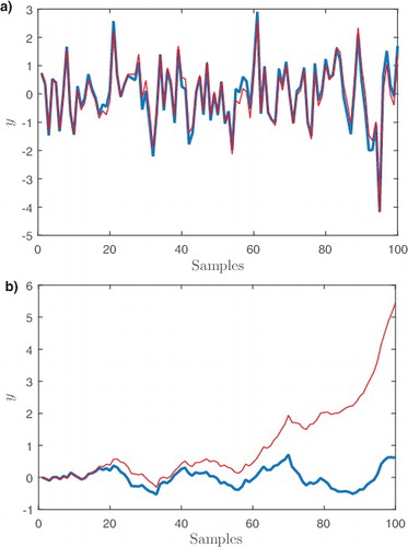The resultant ${\mathcal{H}}_{\infty }$ norm of the forward path system is infinity, as expected from Corollary 3.1, while ‖H _FB (z ⁻¹)‖_∞ = 6.72. The response of both controllers to additive Gaussian white noise at the plant input d(k) or plant output n(k) are shown in Figure 3. With noise at the plant input, the closed-loop response of the forward path controller is unstable, as expected from the observations in Section 3.

Figure 3. Forward path (thin trace, red) and feedback (thick trace, blue) PIP control of the unstable plant. (a) Output responses with d = 0 and zero mean, σ² = 1, Gaussian white noise n at the plant output. (b) Output responses with n = 0 and zero mean, σ² = 1, Gaussian white noise d at the plant input.

4.2 Simple stable plant

The ${\mathcal{H}}_{\infty }$ norm for a simple stable plant, again based on Equation (35(35) $$\begin{array}{c}\hfill y\left(k\right)=\frac{b_1{z}^{-1}}{1+a_1{z}^{-1}}u\left(k\right)\end{array}$$(35) ), is determined for a range of controller gains (and associated desired pole locations). Initially the poles are constrained to be real, repeated, and the plant parameters b ₁ = 0.1 and a ₁ = 0.55 are deliberately chosen (as an illustrative scenario) such that the polynomial Equation (40(40) $$\begin{array}{c}\hfill c_4{p}^4+c_3{p}^3+c_1{p}^2+c_{1}p+c_0=0\end{array}$$(40) ) yields real roots. In this case, the bounds of the roots of Equation (40(40) $$\begin{array}{c}\hfill c_4{p}^4+c_3{p}^3+c_1{p}^2+c_{1}p+c_0=0\end{array}$$(40) ) yield the range of closed-loop poles that minimise the ${\mathcal{H}}_{\infty }$ norm. These analytically derived bounds are illustrated by the shaded area in Figure 4(a), along with the numerical values of the ${\mathcal{H}}_{\infty }$ norm for a range of repeated, real pole positions. There is an agreement between the analytical and numerical methods. However, if the constraints that the poles are repeated and real are now relaxed, then Equation (40(40) $$\begin{array}{c}\hfill c_4{p}^4+c_3{p}^3+c_1{p}^2+c_{1}p+c_0=0\end{array}$$(40) ) can no longer be used to determine bounds on the poles. Numerical optimisation is used instead, as discussed in Section 3.4, with the results (i.e. 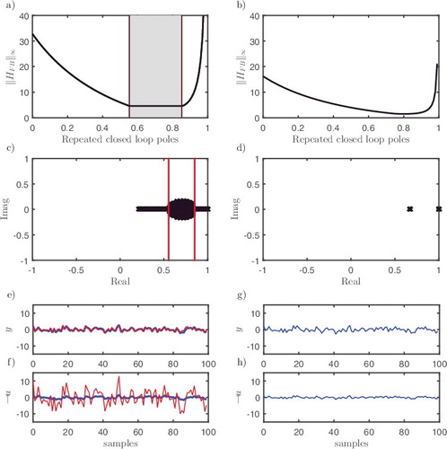pole positions that minimise the ${\mathcal{H}}_{\infty }$ norm) for the present example illustrated in Figure 4(c).

Figure 4. Minimising the ${\mathcal{H}}_{\infty }$ norm of the first-order plant Equation (35(35) $$\begin{array}{c}\hfill y\left(k\right)=\frac{b_1{z}^{-1}}{1+a_1{z}^{-1}}u\left(k\right)\end{array}$$(35) ). (a) Closed-loop poles determined from Equation (40(40) $$\begin{array}{c}\hfill c_4{p}^4+c_3{p}^3+c_1{p}^2+c_{1}p+c_0=0\end{array}$$(40) ) (bounds indicated by shaded region) and numerically determined ‖H _FB ‖_∞ for a range of real, repeated poles (solid trace) when b ₁ = 0.1 and a ₁ = −0.55. (b) Numerically determined ‖H _FB ‖_∞ for a range of repeated closed-loop poles when b ₁ = 0.3 and a ₁ = −0.8. (c) Poles plotted on the complex z-plane that minimise ‖H _FB ‖_∞ when b ₁ = 0.1 and a ₁ = −0.55, together with the constraints determined from Equation (40(40) $$\begin{array}{c}\hfill c_4{p}^4+c_3{p}^3+c_1{p}^2+c_{1}p+c_0=0\end{array}$$(40) ) for real, repeated poles (vertical bounds). (d) Poles plotted on the complex z-plane that minimise ‖H _FB ‖_∞ when b ₁ = 0.3 and a ₁ = −0.8. (e) Output y and (f) control input −u, for b ₁ = 0.1 and a ₁ = −0.55 when the ${\mathcal{H}}_{\infty }$ norm is minimised, showing the case that the ${\mathcal{H}}_2$ norm is maximised (thin trace, red) and minimised (thick trace, blue). (g) Output y and (h) control input −u, for b ₁ = 0.3 and a ₁ = −0.8 when the ${\mathcal{H}}_{\infty }$ norm is minimised.

Even with the repeated, real pole constraints in place, if the polynomial Equation (40(40) $$\begin{array}{c}\hfill c_4{p}^4+c_3{p}^3+c_1{p}^2+c_{1}p+c_0=0\end{array}$$(40) ) does not yield real roots, then we cannot use this expression to find bounds on the poles. Numerical optimisation remains an option, as illustrated in Figure 4(b,d) . A numerical example showing ‖H _FB ‖_∞ for a range of repeated, real pole positions when b ₁ = 0.3 and a ₁ = −0.8 is illustrated in Figure 4(b). Relaxing the constraint on the design poles, Figure 4(d) shows the estimated closed-loop poles that minimise the ${\mathcal{H}}_{\infty }$ norm. In this case, the closed-loop poles converge around a single optimal solution.

For certain plant parameters, such as a ₁ = −0.55 and b ₁ = 0.1 discussed above, it is clear that a range of closed-loop poles (and hence an associated range of possible controller gains) minimises the ${\mathcal{H}}_{\infty }$ norm. This result is illustrated by the ‘flat’ part of the ${\mathcal{H}}_{\infty }$ norm trace in Figure 4(a) but also applies when unconstrained poles are utilised. Optimal poles from the set given in Figure 4(c) that minimise the ${\mathcal{H}}_{\infty }$ norm, are subsequently selected by determining the poles within this set that yield the smallest ${\mathcal{H}}_2$ norm. For the present example, based on a ₁ = −0.55 and b ₁ = 0.1, these poles are p ₁ = 0.27 and p ₂ = 0.96. As a comparison, poles within the set with the largest ${\mathcal{H}}_2$ norm are also determined, i.e. p ₁ = 0.63 + 0.1j and p ₂ = 0.63 − 0.1j. The closed-loop responses, i.e. the generalised outputs ζ when the ${\mathcal{H}}_2$ norm is minimised, are compared to the case when the ${\mathcal{H}}_2$ norm is maximised in Figure 4(e,f) . Minimising the ${\mathcal{H}}_2$ norm yields a significantly smaller magnitude, smoother control input (u) in this case. Similar output responses are shown in Figure 4(g,h) for the plant with b ₁ = 0.3 and a ₁ = −0.8 (the optimal closed-loop poles converge around a single solution hence only one set of responses are shown).

4.3 Stable plant with frequency weighting

We use a weighting filter for low-frequency additive disturbances at the plant input d, in order to estimate poles (and associated PIP control gains) that minimise the ${\mathcal{H}}_{\infty }$ norm for the plant in Equation (35(35) $$\begin{array}{c}\hfill y\left(k\right)=\frac{b_1{z}^{-1}}{1+a_1{z}^{-1}}u\left(k\right)\end{array}$$(35) ) with b ₁ = 0.1 and a ₁ = −0.55. This is achieved using a third order, low pass, Butterworth filter D _d /C _d , where D _d (z ⁻¹) = 0.0004 + 0.0012z ⁻¹ + 0.0012z ⁻² + 0.0004z ⁻³ and C _d (z ⁻¹) = 1.0000 − 2.6862z ⁻¹ + 2.4197z ⁻² − 0.7302z ⁻³ are chosen by trial and error for the purpose of this example. Additive noise at the plant output is ignored, hence D _n /C _n = 0. To evaluate the effect of including a frequency weighting, the input n(k) is set to zero, while d(k) is represented using both filtered (using the filter described above) and unfiltered Gaussian white noise with variance σ² = 1. For comparison, the ${\mathcal{H}}_{\infty }$ norm is minimised with and without frequency weightings for both the filtered and unfiltered disturbances, with the results illustrated in Figure 5. When there are no frequency weightings, a range of gains that minimise the ${\mathcal{H}}_{\infty }$ norm arises, similar to the previous example, hence the optimal gains are determined by also minimising the ${\mathcal{H}}_2$ norm.

Figure 5. The effect of including frequency weightings when minimising the ${\mathcal{H}}_{\infty }$ norm. (a) Filtered disturbance input; (b) output and (d) control input in response to a filtered disturbance when the frequency weighting is not used to minimise the ${\mathcal{H}}_{\infty }$ norm; (c) output and (e) control input in response to a filtered disturbance when the frequency weighting is used to minimise the ${\mathcal{H}}_{\infty }$ norm. (f) Unfiltered, Gaussian white noise disturbance input; (g) output and (i) control input in response to an unfiltered disturbance when the frequency weighting is not used to minimise the ${\mathcal{H}}_{\infty }$ norm; (h) output and (j) control input in response to an unfiltered disturbance when the frequency weighting is used to minimise the ${\mathcal{H}}_{\infty }$ norm.

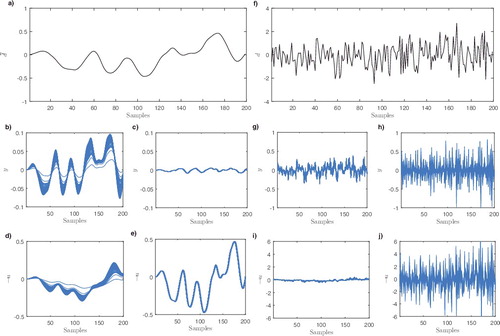
To investigate model uncertainty in the simulation study, the plant parameters are varied from the nominal values (used for PIP control system design) using Monte-Carlo simulation, with 50 realisations based on a diagonal covariance matrix $\mathcal{N}$, and diagonal elements all 10⁻⁴. Figure 5(b–e) compares the generalised errors, ζ = (y, −u), when the ${\mathcal{H}}_{\infty }$ norm is minimised without (Figure 5(b,d)) and with (Figure 5(c,e)) frequency weighting, for the case that the disturbance input is filtered (Figure 5(a)). For this example, use of the frequency weighting approach proposed in Section 3.6 successfully minimises the effect of the low-frequency disturbance inputs on the magnitude of the output y. It also yields reduced variations between the responses when the plant parameters are varied, i.e. improved robustness to model mismatch represented by the smaller envelope of Monte Carlo realisations. By contrast, Figure 5(g–j) compares the generalised errors when the disturbance input is not filtered, i.e. the disturbance is Gaussian white noise (Figure 5(f)). In this case, the generalised errors (y, −u) are greater when including the frequency weighting (using the filter described above) in the optimisation, i.e. as expected, the more robust solution is to use the unweighted approach based on Gaussian noise inputs. To conclude, the frequency weighting approach can be used to improve the robustness of the system to certain types of generalised input signals, ω = (n, d), which is useful in cases when these input signals can be well described as appropriately modelled noise.

4.4 Higher order plant (hair dryer model)

The ${\mathcal{H}}_{\infty }$ norm for a more complex plant model, Equation (42(42) $$\begin{array}{c}\hfill y\left(k\right)={\displaystyle \frac{b_2{z}^{-2}+b_3{z}^{-3}+b_4{z}^{-4}}{1+a_1{z}^{-1}+a_2{z}^{-2}}}u\left(k\right)+\frac{1}{1+c_1{z}^{-1}}e\left(k\right)\end{array}$$(42) ), is considered. This example is based on the Ljung (1987) laboratory hair dryer system. A fan blows heated air through a tube and the air temperature is measured by a thermocouple at the outlet. The input and output variables are the voltage over the heating device (a mesh of resistor wires) and the voltage from the thermocouple, respectively. The sampling interval is Δt = 0.08 s. The plant model is adapted from a Box–Jenkins model with an auto-regressive noise term that has been identified from the experimental data (available in the MATLAB System Identification Toolbox) using the optimal refined instrumental variable (RIV) algorithm (Taylor et al., 2013; Young, 2012): (42) $$\begin{array}{c}\hfill y\left(k\right)={\displaystyle \frac{b_2{z}^{-2}+b_3{z}^{-3}+b_4{z}^{-4}}{1+a_1{z}^{-1}+a_2{z}^{-2}}}u\left(k\right)+\frac{1}{1+c_1{z}^{-1}}e\left(k\right)\end{array}$$(42) where a ₁ = −1.3145, a ₂ = 0.4325, b ₂ = 0.0017, b ₃ = 0.0655, b ₄ = 0.0406, c ₁ = −0.9230 and e(k) is Gaussian white noise with σ² = 0.00142. To calculate the weighted ${\mathcal{H}}_{\infty }$ norm, we use the noise filter, Equation (32(32) $$\begin{array}{c}\hfill n\left(k\right)=\frac{D_n\left(z^{-1}\right)}{C_n\left(z^{-1}\right)}\bar{n}\left(k\right)\end{array}$$(32) ) with D _n (z ⁻¹) = 0.0014 and C _n (z ⁻¹) = 1 − 0.923z ⁻¹. We assume the additive disturbance at the plant input d is Gaussian white noise with σ² = 0.01, hence the weighting filter D _d /C _d = 0.01.

The weighted ${\mathcal{H}}_{\infty }$ norm, expressed in Equation (29(29) $$\begin{array}{c}\hfill \parallel H_{wt}\left(z^{-1}\right){\parallel }_{\infty }=\underset{\theta \in (0,2\pi )}{sup}\sqrt{{\bar{O}}_{wt}{O}_{wt}+{\bar{R}}_{wt}{R}_{wt}+{\bar{Q}}_{wt}{Q}_{wt}+{\bar{E}}_{wt}{E}_{wt}}\end{array}$$(29) ), is used to numerically estimate the controller parameters that minimise the ${\mathcal{H}}_{\infty }$ norm. A wide range of poles (and so control gains) are found to minimise the ${\mathcal{H}}_{\infty }$ norm, as illustrated in Figure 6(a). Therefore, the poles (from the set that minimises the ${\mathcal{H}}_{\infty }$ norm) that both minimise and (for comparison purposes) maximise the ${\mathcal{H}}_2$ norm are determined. The response to filtered exogenous input signals, when using the filters described above, are illustrated in Figure 6(b). Jointly minimising the ${\mathcal{H}}_{\infty }$ norm and ${\mathcal{H}}_2$ norm for this simulation example yields a relatively very low variance control input signal (implying reduced actuator wear and tear in some applications). Whilst the ${\mathcal{H}}_{\infty }$ norm reflects the worst case, or maximum amplification at a single frequency between the errors and exogenous inputs, the ${\mathcal{H}}_2$ norm represents amplification over all frequencies. In this example, maximum amplification across all frequencies occurs when θ = 0, hence introducing the ${\mathcal{H}}_2$ norm ensures that the gain over all frequencies is reduced, yielding the significantly smaller input amplitudes seen in Figure 6(b).

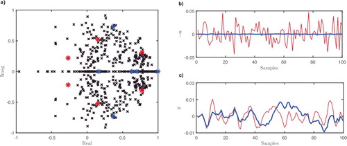
Figure 6. Minimising the ${\mathcal{H}}_{\infty }$ norm of the hair dryer model. Results when the ${\mathcal{H}}_2$ norm is minimised (thick trace, blue) and maximised (thin trace, red) are both shown. (a) Estimated poles plotted on the complex z-plane that minimise the ${\mathcal{H}}_{\infty }$ norm. (b) Control input response and (c) output response to filtered noise n and disturbance d.

5. Experimental example

To demonstrate the practical utility of the proposed approach, the final example concerns control of the air velocity within a 2 m by 1 m by 1 m ventilation chamber at Lancaster University. The chamber contains an array of 30 thermocouples, air velocity transducers at the inlet and outlet, and three actuators, namely axial fans at the inlet and outlet, and a 400 W heating element, used to generate various micro-climatic conditions within the chamber. Operation of the chamber is controlled by National Instruments hardware/software, with the control input signals in the range 0–5 V in each case. For more information, see, e.g. Tsitsimpelis and Taylor (2015) and the references therein.

The outlet ventilation rate is usually controlled via the outlet axial fan. However, to increase the control challenge for the purpose of the present article, the outlet axial fan u(k) is instead used to control the inlet air velocity v(k), increasing the noise and uncertainties involved in the system dynamics. In fact, to use the reduced block diagram form in Figure 2(a), the controlled output y(k) = v(k) − y ₀ where y ₀ is an off-set to allow for non-zero reference inputs. To identify the control model, a pseudo-random-binary-signal with 1 Hz sampling frequency is applied to the fan, and the airflow is measured at the same sampling frequency. Use of Young's Information Criteria and the RIV algorithm (Taylor et al., 2013; Young, 2012), both implemented within the CAPTAIN toolbox (Taylor, Pedregal, Young, & Tych, 2007), yields the following model for air velocity at the inlet: (43) $$\begin{array}{c}\hfill y\left(k\right)={\displaystyle \frac{b_2{z}^{-2}}{1+a_1{z}^{-1}}}u\left(k\right)\end{array}$$(43) The identified model is based on Equation (1(1) $$\begin{array}{c}\hfill y\left(k\right)=\frac{B\left(z^{-1}\right)}{A\left(z^{-1}\right)}u\left(k\right)=\frac{b_1{z}^{-1}+\cdots +b_m{z}^{-m}}{1+a_1{z}^{-1}+\cdots +a_n{z}^{-n}}u\left(k\right)\end{array}$$(1) ), with n = 1, m = 2 and b ₁ = 0, i.e. there are two samples pure time delay. The time delay is automatically compensated for by the third-order NMSS representation in this case, based on x (k) = [y(k)~u(k − 1)~q(k)]^⊺and the associated PIP control elements, F(z ⁻¹) = f ₀, G(z ⁻¹) = 1 + g ₁ z ⁻¹ and k _I /Δ.

Following a similar approach to the earlier examples, values of the PIP control gains that minimise the ${\mathcal{H}}_{\infty }$ norm are estimated numerically, with the results shown in Table 1. Initially, the minimal ${\mathcal{H}}_{\infty }$ norm yields an integral gain k _I = 0, which is unsatisfactory in practice since the controller would not ensure Type 1 servomechanism performance. The present example addresses step changes in the reference signal for a real (nonlinear) system, hence for good steady-state control performance, low-frequency signals have increased importance. Therefore, using the frequency weighting approach described in Section 3.6, a low-pass filter 0.1z ⁻¹/(1 − 0.98z ⁻¹) is designed, and the PIP control gains that minimise the weighted ${\mathcal{H}}_{\infty }$ norm, and within this set the ${\mathcal{H}}_2$ norm, are determined. For comparison, PIP controllers are designed using standard pole placement and LQ methods without considering robustness in terms of the ${\mathcal{H}}_{\infty }$ norm. For pole placement, closed-loop poles were placed at 0.6, 0.7, 0.8 to obtain a relatively fast response, while for LQ optimisation two options are considered: (1) with the control weights set to unity (the ‘default’ in many applications) and (2) with the weight for the integral-of-error state reduced to 0.1 to obtain a slower response; see Chapter 5 in Taylor et al. (2013) for details. The corresponding control gains are listed in Table 1.

Table 1. Model parameters and various PIP control designs for the ventilation chamber. The control model is defined by Equation (43(43) $$\begin{array}{c}\hfill y\left(k\right)={\displaystyle \frac{b_2{z}^{-2}}{1+a_1{z}^{-1}}}u\left(k\right)\end{array}$$(43) ). The coefficient of determination Rt² provides a measure of the model fit, where Rt² = 1.0 indicates an exact fit to the data. PIP control parameters (i.e. control gains and associated pole positions) are estimated using the ${\mathcal{H}}_{\infty }$ norm, the weighted ${\mathcal{H}}_{\infty }$ norm, pole placement and LQ optimisation. The closed-loop poles refer to the poles of the closed-loop system when there is no model mismatch. For example, the weighted ${\mathcal{H}}_{\infty }$ approach yields control gains f ₀ = 0.8, g ₁ = −0.3 and k _I = 0.06, and these gains are utilised to determine the poles 0.94, 0.73 and 0.56. For LQ design, W _e is the weight associated with the integral-of-error state variable.

Model	a 1	−0.92
parameters	b 2	0.13
Model fit	Rt^2	0.976
	${\mathcal{H}}_{\infty }$	1.00, 0.88, −0.49
Closed-loop	Weighted ${\mathcal{H}}_{\infty }$	0.94 0.73 0.56
poles	Pole placement	0.6, 0.7, 0.8
	LQ (W e = 1)	0.00, 0.74 ± 0.18i
	LQ (W e = 0.1)	0.00, 0.84 ± 0.10i
	${\mathcal{H}}_{\infty }$	0.47, 0.53, 0.00
PIP control	Weighted ${\mathcal{H}}_{\infty }$	0.80, −0.30, 0.06
gains	Pole placement	1.34, −0.18, 0.19
(f 0, g 1, k I )	LQ (W e = 1)	3.18, 0.44, 0.79
	LQ (W e = 0.1)	1.72 0.24 0.28

Earlier articles (e.g. Tsitsimpelis & Taylor, 2015) demonstrate a nonlinear relationship between fan input voltage and steady-state air velocity, hence the standard concept of selecting an operating condition for designing a linear controller is important. To investigate the significance of ${\mathcal{H}}_{\infty }$ design, the design operating condition and associated control model, Equation (43(43) $$\begin{array}{c}\hfill y\left(k\right)={\displaystyle \frac{b_2{z}^{-2}}{1+a_1{z}^{-1}}}u\left(k\right)\end{array}$$(43) ), are deliberately based on a relatively low magnitude input, 1 − 2 V, associated with steady-state air velocities of approximately 1 m/s, while the controllers are evaluated for reference outputs in the range 0 − 4 m/s, as shown in Figure 7. This represents significant model mismatch in practice and is the reason for the oscillatory responses observed, particularly for the controllers designed without considering robustness. 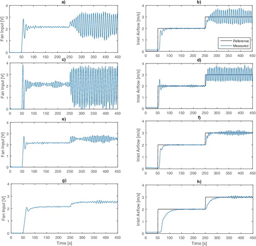By contrast, the response of the controller designed using the weighted ${\mathcal{H}}_{\infty }$ norm yields a slower response time but is less oscillatory (Figure 7(g,h)), especially over the last 200 s where the model mismatch is greatest.

Figure 7. Experimental results showing the control input (left-hand side subplots) and output (right) for each PIP control algorithm. The controllers are all based on an air velocity operating condition of approximately 1 m/s but the reference signal is 0 for 50 s, 2 m/s for 200 s and 3 m/s for a further 200 s. (a) Control input and (b) output for pole placement. (c) Control input and (d) output for LQ optimisation with unity weights. (e) Control input and (f) output for LQ optimisation with the integral-of-error weight set to 0.1 and the other weights unity. (g) Control input and (h) output using the weighted ${\mathcal{H}}_{\infty }$ norm.

6. Conclusions

The article has presented new analytical expressions for evaluating the robustness of feedback and forward path PIP control. The robustness of the closed-loop system is a key concern when controlling real systems that are subject to uncertainty. Our analytical expressions are used to evaluate the robustness of existing PIP controllers, as well as to provide an additional design constraint for determining control gains that result in a more robust closed-loop system.

The forward path PIP structure was originally introduced to provide smoother input signals for some types of control problem (Taylor et al., 1998). However, the present article shows that it is not robust when the controlled system is unstable. Moreover, methods to jointly minimise the ${\mathcal{H}}_{\infty }$ and ${\mathcal{H}}_2$ norms, as developed in this article, provide an alternative way to reduce the variance of the control input signals, while using the more robust, feedback PIP control structure: see Figure 6(b) for an example. More generally, the ${\mathcal{H}}_{\infty }$ norm (or weighted ${\mathcal{H}}_{\infty }$ norm) provides an alternative model-based approach to tuning the PIP control gains, in comparison to trial and error adjustment of the pole positions or optimal LQ design. Nonetheless, the PIP algorithm obtained in this way has the same, relatively straightforward implementation form as the conventional PIP approach, often with a similar degree of complexity to PI/PID control.

Each design approach (e.g. LQ, pole placement and ${\mathcal{H}}_{\infty }$ norm) represents a model-based method to determine the gains of the PIP control system, based on the ‘desired’ performance of the closed-loop system. For the pole assignment method, performance relates to the poles of the closed-loop system, for LQ optimisation, it is the minimisation of the ubiquitous LQ cost function, and for ${\mathcal{H}}_{\infty }$ optimisation, the minimisation of the ${\mathcal{H}}_{\infty }$ norm of the closed-loop system. Of course, each method could produce the same outcome if the design criteria are set ‘correctly’. For example, the conventional PIP pole assignment algorithm (Taylor et al., 2013) can be utilised to set the closed-loop poles corresponding to the poles that minimise the ${\mathcal{H}}_{\infty }$ norm (once these are known). Hence, it can be argued that the choice of poles, LQ weights and the weighting filter used in the ventilation control example (Section 5) are somewhat arbitrary. However, the advantage of the ${\mathcal{H}}_{\infty }$ design criteria is that it provides a quantitative method of determining the closed-loop poles (or equivalently control gains) that result in a robust control design.

Classical solutions of the ${\mathcal{H}}_{\infty }$ control problem usually refer to the full order case, where the size and structure of the controller is not constrained. By contrast, the expressions given in this article are for a specific form of the controller, i.e. PIP control. As a result, the comparative study presented here concerns different approaches to selecting the control coefficients (${\mathcal{H}}_{\infty }$, LQ and pole assignment) within this constrained case. Nonetheless, the relationship between PIP ${\mathcal{H}}_{\infty }$ control and other ${\mathcal{H}}_{\infty }$ approaches (e.g. Grimble, 1989; Kwakernaak, 1993) will be investigated in future work.

The ${\mathcal{H}}_{\infty }$ approach is most useful in cases where large uncertainties are involved, and stability across a range of operating conditions is required. However, the examples in this article show that the increased robustness is often synonymous with slower performance; in other words, they demonstrate the classical trade-off between speed of response and robustness. Therefore, in cases when the model is well defined and there are no significant sources of noise, a ‘non-robust’ (e.g. LQ optimal) solution is likely to provide better performance in terms of settling times. Finally, where there are multiple constraints on the closed-loop performance, the ${\mathcal{H}}_{\infty }$ norm can be used in combination with multi-objective optimisation techniques (e.g. Exadaktylos & Taylor, 2010) to provide the most robust design (in terms of the ${\mathcal{H}}_{\infty }$ norm) that also meets defined performance criteria, and this is the subject of on-going research by the authors.

Disclosure statement

No potential conflict of interest was reported by the authors.

Additional information

Funding

This work is supported by the UK Engineering and Physical Sciences Research Council (EPSRC) [grant number EP/M015637/1].

Appendix

The elements of the NMSS equations (given in Equation (2(2) $$\begin{array}{c}\hfill \mathit{x}\left(k\right)=\mathit{F}\mathit{x}(k-1)+\mathit{g}u(k-1)+\mathit{d}{y}_d\left(k\right);y\left(k\right)=\mathit{h}\mathit{x}\left(k\right)\end{array}$$(2) )) are defined in this Appendix. The state transition matrix F , input vector g , command input vector d and output vector h are (A1) $$\begin{array}{c}\hfill \mathit{F}=\left[\begin{array}{ccccccccccc}-a_1& -a_2& \cdots & -a_{n-1}& -a_n& b_2& b_3& \cdots & b_{m-1}& b_m& 0\\ 1& 0& \cdots & 0& 0& 0& 0& \cdots & 0& 0& 0\\ 0& 1& \cdots & 0& 0& 0& 0& \cdots & 0& 0& 0\\ ⋮& ⋮& \ddots & ⋮& ⋮& ⋮& ⋮& \ddots & ⋮& ⋮& ⋮\\ 0& 0& \cdots & 1& 0& 0& 0& \cdots & 0& 0& 0\\ 0& 0& \cdots & 0& 0& 0& 0& \cdots & 0& 0& 0\\ 0& 0& \cdots & 0& 0& 1& 0& \cdots & 0& 0& 0\\ 0& 0& \cdots & 0& 0& 0& 1& \cdots & 0& 0& 0\\ ⋮& ⋮& \ddots & ⋮& ⋮& ⋮& ⋮& \ddots & ⋮& ⋮& ⋮\\ 0& 0& \cdots & 0& 0& 0& 0& \cdots & 1& 0& 0\\ a_1& a_2& \cdots & a_{n-1}& a_n& -b_2& -b_3& \cdots & -b_{m-1}& -b_m& 1\end{array}\right]\end{array}$$(A1) (A2) $$\begin{array}{c}\hfill \mathit{g}={\left[\begin{array}{ccccccccccc}{b}_1& 0& 0& \cdots & 0& 0& 0& 0& \cdots & 0& -b_1\end{array}\right]}^{⊺}\end{array}$$(A2) (A3) $$\begin{array}{c}\hfill \mathit{d}={\left[\begin{array}{ccccccccccc}0& 0& 0& \cdots & 0& 0& 0& 0& \cdots & 0& 1\end{array}\right]}^{⊺}\end{array}$$(A3) (A4) $$\begin{array}{c}\hfill \mathit{h}=\left[\begin{array}{ccccccccccc}1& 0& \cdots & 0& 0& 0& 0& \cdots & 0& 0& 0\end{array}\right]\end{array}$$(A4)

References

- Åström, K. J. , Panagopoulos, H. , & Hägglund, T. (1998). Design of PI controllers based on non-convex optimization. Automatica , 34 (5), 585–601.
- Bernstein, D. S. , & Haddad, W. M. (1989). LQG control with an H ∞ performance bound: A Riccati equation approach. IEEE Transactions on Automatic Control , 34 (3), 293–305.
- Bigdeli, N. (2015). The design of a non-minimal state space fractional-order predictive functional controller for fractional systems of arbitrary order. Journal of Process Control , 29 , 45–56.
- Clairon, Q. , Wilson, E. D. , Henderson, R. , & Taylor, C. J. (2017). Adaptive biomedical treatment and robust control. IFAC-PapersOnLine, 50(1), 12191–12196.
- Exadaktylos, V. , & Taylor, C. J. (2010). Multi-objective performance optimisation for model predictive control by goal attainment. International Journal of Control , 83 (7), 1374–1386.
- Fletcher, I. , Wilson, I. , & Cox, C. S. (1994). A comparison of some multivariable design techniques using a coupled tanks experiment. In R. Whalley (Ed.), Application of multivariable system techniques (pp. 49–60). London: Mechanical Engineering Publications Limited.
- Francis, B. A. (1987). Lecture notes in control and information sciences. A Course in H∞ Control Theory . Berlin: Springer-Verlag.
- Goncalves, E. N. , Palhares, R. M. , & Takahashi, R. H. (2008). A novel approach for H2 / H∞ robust PID synthesis for uncertain systems. Journal of Process Control , 18 (1), 19–26.
- Green, M. , & Limebeer, D. J. (2012). Linear robust control . New York: Dover Publications, Inc.
- Grimble, M. J. (1989). Generalised H∞ multivariable controllers. IEE Proceedings D , 136 (6), 285–297.
- Ho, M.-T. (2003). Synthesis of H ∞ PID controllers: A parametric approach. Automatica , 39 (6), 1069–1075.
- Ho, M.-T. , & Lu, J.-M. (2005). H ∞ PID controller design for lur’e systems and its application to a ball and wheel apparatus. International Journal of Control , 78 (1), 53–64.
- Khalilipour, M. M. , Sadeghi, J. , Shahraki, F. , & Razzaghi, K. (2016). Nonsquare multivariable non-minimal state space-proportional integral plus (NMSS-PIP) control for atmospheric crude oil distillation column. Chemical Engineering Research and Design , 113 , 140–150.
- Khargonekar, P. P. , & Rotea, M. A. (1991). Mixed H 2 and H ∞ control: A convex optimization approach. IEEE Transactions on Automatic Control , 36 (7), 824–837.
- Kristiansson, B. , & Lennartson, B. (2002). Robust and optimal tuning of PI and PID controllers. IEE Proceedings: Control Theory and Applications , 149 (1), 17–25.
- Kwakernaak, H. (1993). Robust control and H-∞ optimization-tutorial paper. Automatica , 29 (2), 255–273.
- Liu, G. , Dixon, R. , & Daley, S. (2001). Design of stable proportional-integral-plus controllers. International Journal of Control , 74 (16), 1581–1587.
- Liu, G. , Duan, G. , & Dixon, R . (2001). Robust control with stable proportional-integral-plus controllers. In 2001 European Control Conference (ECC) , (pp. 3201–3206).
- Ljung, L. (1987). System identification, theory for the user . Englewood Cliffs, NJ: Prentice Hall.
- Palhares, R. , Taicahashi, R. , & Peres, P. L. (1997). H-∞ and H2 guaranteed costs computation for uncertain linear systems. International Journal of Systems Science , 28 (2), 183–188.
- Quanten, S. , McKenna, P. , Van Brecht, A. , Van Hirtum, A. , Young, P. , Janssens, K. , & Berckmans, D. (2003). Model-based PIP control of the spatial temperature distribution in cars. International Journal of Control , 76 (16), 1628–1634.
- Seward, D. , Scott, J. , Dixon, R. , Findlay, J. , & Kinniburgh, H. (1997). The automation of piling rig positioning using satellite GPS. Automation in Construction , 6 (3), 229–240.
- Shaban, E. M. , Ako, S. , Taylor, C. J. , & Seward, D. W. (2008). Development of an automated verticality alignment system for a vibro-lance. Automation in Construction , 17 (5), 645–655.
- Stoorvogel, A. A. (1992). The discrete time H ∞ control problem with measurement feedback. SIAM Journal on Control and Optimization , 30 (1), 182–202.
- Taylor, C. J. , Chotai, A. , & Cross, P. (2012). Non-minimal state variable feedback decoupling control for multivariable continuous-time systems. International Journal of Control , 85 (6), 722–734.
- Taylor, C. J. , Chotai, A. , & Young, P. C. (1998). Proportional-integral-plus (PIP) control of time delay systems. IMECHE Proceedings Part I: Journal of Systems and Control Engineering , 212 (1), 37–48.
- Taylor, C. J. , Chotai, A. , & Young, P. C. (2000). State space control system design based on non-minimal state-variable feedback: Further generalization and unification results. International Journal of Control , 73 (14), 1329–1345.
- Taylor, C. J. , Leigh, P. , Price, L. , Young, P. , Vranken, E. , & Berckmans, D. (2004). Proportional-integral-plus (PIP) control of ventilation rate in agricultural buildings. Control Engineering Practice , 12 (2), 225–233.
- Taylor, C. J. , Pedregal, D. J. , Young, P. C. , & Tych, W. (2007). Environmental time series analysis and forecasting with the Captain toolbox. Environmental Modelling & Software , 22 (6), 797–814.
- Taylor, C. J. , Young, P. C. , & Chotai, A. (1996). PIP optimal control with a risk sensitive criterion. In Control '96, UKACC International Conference , IEE Conference Publication No. 427.
- Taylor, C. J. , Young, P. C. , & Chotai, A. (2013). True digital control: Statistical modelling and non-minimal state space design. Chichester, UK: John Wiley & Sons, Ltd.
- Toivonen, H. , & Pensar, J. (1996). A worst-case approach to optimal tracking control with robust performance. International Journal of Control , 65 (1), 17–32.
- Tsitsimpelis, I. , & Taylor, C. J. (2015). Partitioning of indoor airspace for multi-zone thermal modelling using hierarchical cluster analysis. In 2015 European Control Conference (ECC) . Linz, Austria.
- Valério, D. , & da Costa, J. S. (2006). Tuning of fractional controllers minimising H 2 and H ∞ norms. Acta Polytechnica Hungarica , 3 (4), 55–70.
- Wang, L. , & Young, P. C. (2006). An improved structure for model predictive control using non-minimal state space realisation. Journal of Process Control , 16 (4), 355–371.
- Whittle, P. (1981). Risk sensitive linear/quadratic/gaussian control. Advances in Applied Probability , 13 , 764–777.
- Yeh, H.-H. , Banda, S. S. , & Chang, B.-C. (1992). Necessary and sufficient conditions for mixed H 2 and H∞ optimal control. IEEE Transactions on Automatic Control , 37 (3), 355–358.
- Young, P. C. (2012). Recursive estimation and time-series analysis: An introduction . Berlin: Springer-Verlag.
- Young, P. , Behzadi, M. , Wang, C. , & Chotai, A. (1987). Direct digital and adaptive control by input-output state variable feedback pole assignment. International Journal of Control , 46 (6), 1867–1881.
- Yucelen, T. , & Pourboghrat, F . (2009). Active noise blocking: Non-minimal modeling, robust control, and implementation. In 2009 American control conference (pp. 5492–5497).
- Zames, G. (1981). Feedback and optimal sensitivity: Model reference transformations, multiplicative seminorms, and approximate inverses. IEEE Transactions on Automatic Control , 26 (2), 301–320.
- Zhang, R. , & Gao, F. (2013). Multivariable decoupling predictive functional control with non-zero-pole cancellation and state weighting: Application on chamber pressure in a coke furnace. Chemical Engineering Science , 94 , 30–43.
- Zhou, K. , & Doyle, J. C . (1998). Essentials of robust control . Upper Saddle River, NJ: Prentice Hall.
- Zhou, K. , Doyle, J. C. , Glover, K. (1996). Robust and optimal control . New Jersey, NJ: Prentice Hall.