Tensor networks for MIMO LPV system identification

ABSTRACT

In this paper, we present a novel multiple input multiple output (MIMO) linear parameter varying (LPV) state-space refinement system identification algorithm that uses tensor networks. Its novelty mainly lies in representing the LPV sub-Markov parameters, data and state-revealing matrix condensely and in exact manner using specific tensor networks. These representations circumvent the ‘curse-of-dimensionality’ as they inherit the properties of tensor trains. The proposed algorithm is ‘curse-of-dimensionality’-free in memory and computation and has conditioning guarantees. Its performance is illustrated using simulation cases and additionally compared with existing methods.

KEYWORDS:

• Identification
• LPV systems
• tensor trains
• subspace methods
• closed-loop identification
• time-varying systems

1. Introduction

In this paper, the focus is on linear parameter varying (LPV) systems. Because these systems are able to describe time-varying and non-linear systems, while allowing for powerful properties extended from linear system theory. Also, there are control design methods which can guarantee robust performance (Scherer, 2001), and several convex and non-convex identification methods exist. The dynamics of LPV systems are a function of the scheduling sequence, which contains the time-varying and non-linear effects. In this paper, we focus on affine functions of known arbitrary scheduling sequences, which are relevant to wind turbine applications (Bianchi, Mantz, & Christiansen, 2005; Gebraad, van Wingerden, Fleming, & Wright, 2011; van Wingerden & Verhaegen, 2009). Other applications are aircraft applications (Balas, 2002), compressors (Giarré, Bauso, Falugi, & Bamieh, 2006), batteries (Remmlinger, Buchholz, & Dietmayer, 2013) and wafer stages (van der Maas, van der Maas, & Oomen, 2015; Wassink, van de Wal, Scherer, & Bosgra, 2005). The scheduling sequence can be any function of known variables. This representation allows us for example to take the effect of blade position on gravity forces and blade rotational speed into account (Gebraad, van Wingerden, Fleming, & Wright, 2013).

In this paper, the focus is on LPV identification methods. That is, from input–output and scheduling data we try to estimate an LPV model of the system. This model can then be used to design a controller. Several methods exist, which can be divided in two different ways. Firstly, global and local methods can be distinguished (De Caigny, Camino, & Swevers, 2009; Shamma, 2012; Tóth, 2010). Local methods utilise that LPV systems act as LTI systems when the scheduling sequence is kept at constant value. These methods identify LTI models at several fixed constant value scheduling sequences and then combine them into an LPV model through interpolation techniques. This does require the application to allow for such experiments. In contrast, global methods use only a single experiment. In this paper, only global methods will be considered. Secondly, input–output (Laurain, Gilson, Tóth, & Garnier, 2010; Tóth, 2010) and state-space methods (Cox & Tóth, 2016; Larimore & Buchholz, 2012; van Wingerden & Verhaegen, 2009; Verdult, Bergboer, & Verhaegen, 2003) exist. The first produces input–output models and the latter state-space models. While in the linear time invariant (LTI) framework these two types of models can be transformed back and forth, in the LPV case this is not trivial and problematic (Tóth, Abbas, & Werner, 2012). In this paper, the focus is on state-space models, because they are the mainstream control design models and can inherently deal with multiple input multiple output (MIMO) problems. More specifically, we focus on predictor-based methods because they can deal with closed-loop data. However, one possible drawback of these methods is the ‘curse-of-dimensionality’.

Namely, the number of to be estimated (LPV sub-Markov) parameters scales exponentially. This can give problems with memory usage and computational cost. Furthermore, the number of parameters can exceed the number of data points, resulting in ill-conditioned problems. Both problems demand special care.

In literature, these problems have been tackled using both convex methods and non-convex refinement methods. Convex methods such as proposed by van Wingerden and Verhaegen (2009) and Gebraad et al. (2011) overcome the memory and computation cost problem by using a dual parametrisation, and address the ill-condition with regularisation. Regularisation is a way to introduce a bias-variance trade-off in estimates. Refinement methods use a non-linear parametrisation with few variables to overcome both problems. However, this returns a non-convex optimisation problem which requires initialisation by an initial estimate. Hence, the goal of refinement methods is to refine initial estimates. The method proposed by Verdult et al. (2003) directly parametrises the state-space matrices for this purpose, and works for open-loop data.

These problems have also been tackled in Gunes, van Wingerden, and Verhaegen (2017) and Gunes, van Wingerden, and Verhaegen (2016). Those two papers and this paper differ in that they use different tensors and different tensor techniques. The different tensor techniques result in vastly different methods. In Gunes et al. (2016), a parameter tensor is constructed whose matricisations are each low-rank. This allows exploitation through nuclear norms and has resulted in a convex subspace method. Tensor techniques are not used to tackle the ‘curse-of-dimensionality’ in that paper. In Gunes et al. (2017), a parameter tensor is constructed which admits a constrained polyadic decomposition and parametrisation. This resulted in a refinement method. However, the computation of the polyadic rank is NP-hard (Håstad, 1990) and approximation with a fixed polyadic rank in the Frobenius norm can be ill-posed (De Silva & Lim, 2008). This method is not ‘curse-of-dimensionality’-free in memory or computation. In this paper, a tensor network approach will be used. The identification problem will be recast and optimised using tensor networks. The major difference with previous work is that this approach uses tensor networks. These allow the method to circumvent the explicit construction of the LPV sub-Markov parameters and makes the proposed refinement method ‘curse-of-dimensionality’-free in memory and computation. This includes a novel technique for constructing the estimate state-revealing matrix directly from the estimate tensor estimate. Notice that both the ‘curse-of-dimensionality’ and novelty lie in the first regression step and in forming the state-revealing matrix. Another difference with Gunes et al. (2016) is that this method is a refinement method, and does not limit the exploitation of the tensor structure to a regularisation term. For completeness, the problem definition is to develop an LPV state-space refinement method which by exploiting underlying tensor network structure is ‘curse-of-dimensionality’-free in memory and computation and successfully refines initial estimates from convex methods.

In this paper, we present the following novel contributions. Firstly, the LPV identification problem is recast and optimised using tensor networks to make the proposed refinement method ‘curse-of-dimensionality’-free in memory and computation. This is done by circumventing the explicit construction of the LPV sub-Markov parameters. Namely, operations can be performed directly on the tensor network decompositions. In detail, the used class of tensor network (Batselier, Chen, & Wong, 2017) is a generalisation of tensor trains (Oseledets, 2011). They inherit tensor train efficiency results, and become tensor trains for single-output problems. These decompositions allow efficient storage and computation in the tensor network domain. This recast in tensor networks includes not only the LPV sub-Markov parameters, but also the data and state-revealing matrix. More specifically, the LPV sub-Markov parameters are shown to admit exact tensor network representation with ranks equal to the model order, and the data tensor admits exact and sparse tensor network representation. Secondly, these properties are exploited to obtain a condensed tensor network parametrisation which can be optimised ‘curse-of-dimensionality’-free in memory and computation. Thirdly, we propose an efficient way to obtain the estimate state sequence from the estimate tensor networks without explicitly constructing the LPV sub-Markov parameters. Additionally, we provide an upper bound on the condition numbers of its sub-problems.

The paper outline is as follows. In Section 3 our LPV identification problem is presented in the tensor network framework. Subsequently in Section 4 a tensor network identification method is proposed. Finally, simulations results and conclusions are presented. In the next section, background is provided on LPV identification and tensor trains (and networks).

2. Background

Before presenting the novel results, relevant topics are reviewed. These topics are LPV identification with state-space matrices, tensor trains and tensor networks. Throughout the paper, for clarity matrices will be denoted by capital characters, tensors which are part of a tensor network decomposition by calligraphic characters and other tensors by bold characters.

2.1. LPV system identification with state-space matrices

In this subsection, LPV system identification with state-space matrices is reviewed (van Wingerden & Verhaegen, 2009). First define the following signals relevant to LPV state-space systems: (1) $x_k\in {\mathbb{R}}^n,u_k\in {\mathbb{R}}^r,y_k\in {\mathbb{R}}^l,{\mu }_k\in {\mathbb{R}}^m,$(1) as the state, input, output and scheduling sequence vector at sample number k. For later use, additionally define (2) $\begin{array}{rl}{\mu }_k& =\left[\begin{array}{ccc}{\mu }_k^{\left(1\right)}& \dots & {\mu }_k^{\left(m\right)}\end{array}\right]{}^T,\\ \mu & =\left[\begin{array}{ccc}{\mu }_1& \dots & {\mu }_N\end{array}\right].\end{array}$(2)

Predictor-based methods (Chiuso, 2007; van Wingerden & Verhaegen, 2009) use the innovation representation and predictor-based representation of LPV state-space systems. Therefore, we directly present the assumed data-generating system as (3a) $x_{k+1}=\sum _{i=1}^m{\mu }_k^{\left(i\right)}\left(A^{\left(i\right)}{x}_k+B^{\left(i\right)}{u}_k+K^{\left(i\right)}{e}_k\right),$(3a) (3b) $y_k=C{x}_k+e_k,$(3b) where the variables $A^{\left(i\right)}$, $B^{\left(i\right)}$, C and $K^{\left(i\right)}$ are appropriately dimensioned state, input, output and observer matrices and $e_k$ is the innovation term at sample k. Notice that the output equation has an LTI C matrix and the feed-through term D is the zero matrix. This assumption is made for the sake of presentation and simplicity of derivation, similar to what has been done in van Wingerden and Verhaegen (2009). This will not trivialise the bottleneck ‘curse-of-dimensionality’. 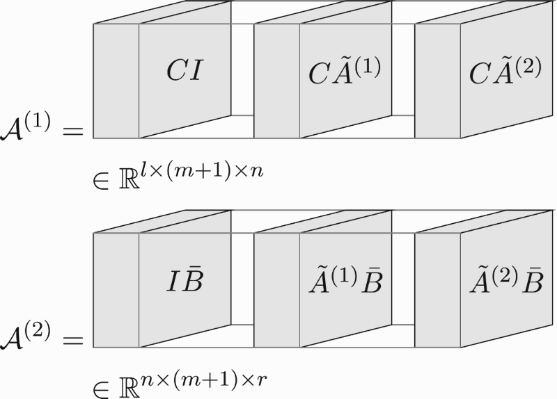Furthermore, it is assumed that ${\mu }_k$ is known and this state-space system has affine dependency on ${\mu }_k$ like in van Wingerden and Verhaegen (2009). That is, ${\mu }_k^{\left(1\right)}=1,\mathrm{\forall }k$. The predictor-based representation follows by substituting (3b(3b) $y_k=C{x}_k+e_k,$(3b) ) in (3a(3a) $x_{k+1}=\sum _{i=1}^m{\mu }_k^{\left(i\right)}\left(A^{\left(i\right)}{x}_k+B^{\left(i\right)}{u}_k+K^{\left(i\right)}{e}_k\right),$(3a) ): (4a) $x_{k+1}=\sum _{i=1}^m{\mu }_k^{\left(i\right)}\left({\tilde{A}}^{\left(i\right)}{x}_k+{\overline{B}}^{\left(i\right)}\left[\begin{array}{c}{u}_k\\ y_k\end{array}\right]\right),$(4a) (4b) $y_k=C{x}_k+e_k,$(4b) where ${\tilde{A}}^{\left(i\right)}$ is $A^{\left(i\right)}-K^{\left(i\right)}C$ and ${\overline{B}}^{\left(i\right)}$ is $[B^{\left(i\right)},K^{\left(i\right)}]$. Notice that the states here are the observer states. Also, define p as a past window for later use. Furthermore, define the discrete-time time-varying transition matrix (van Wingerden & Verhaegen, 2009): (5a) ${\tilde{A}}_k=\sum _{i=1}^m{\mu }_k^{\left(i\right)}{\tilde{A}}^{\left(i\right)},$(5a) (5b) ${\phi }_{j,k}={\tilde{A}}_{k+j-1}\dots {\tilde{A}}_{k+1}{\tilde{A}}_k.$(5b) Predictor-based methods make the assumption that this matrix is exactly zero when j is greater than or equal to the past window p (Chiuso, 2007; van Wingerden & Verhaegen, 2009): (6) ${\phi }_{j,k}\approx 0,\mathrm{\forall }j\ge p.$(6) A similar approximation is also used in several LTI methods (van der Veen, van Wingerden, Bergamasco, Lovera, & Verhaegen, 2013). If the predictor-based system is uniformly exponentially stable, then the approximation error can be made arbitrarily small by increasing p (Knudsen, 2001). In fact the introduced bias disappears as p goes to infinity, but is hard to quantify for finite p (Chiuso, 2007). This assumption results in the predictor-based data equation.

Before presenting this data equation, first some definitions must be given. For ease of presenting matrix sizes, define (7) $q=(l+r)\sum _{j=1}^p{m}^j.$(7) Now define the extended LPV controllability matrix (van Wingerden & Verhaegen, 2009) as (8a) $\begin{array}{rl}{K}_{\left(p\right)}& =[L_p\dots L_2\overline{B}]\in {\mathbb{R}}^{n\times q},\end{array}$(8a) (8b) $\begin{array}{rl}\overline{B}& =[{\overline{B}}^{\left(1\right)}\dots {\overline{B}}^{\left(m\right)}]\in {\mathbb{R}}^{n\times (l+r)m},\end{array}$(8b) (8c) $\begin{array}{rl}{L}_2& =[{\tilde{A}}^{\left(1\right)}\overline{B}\dots {\tilde{A}}^{\left(m\right)}\overline{B}]\in {\mathbb{R}}^{n\times (l+r)m^2},\end{array}$(8c) (8d) $\begin{array}{rl}{L}_{i+1}& =[{\tilde{A}}^{\left(1\right)}{L}_i\dots {\tilde{A}}^{\left(m\right)}{L}_i]\in {\mathbb{R}}^{n\times (l+r)m^{i+1}},\\ & 2\ge i\ge p-1.\end{array}$(8d) For this purpose also define the data matrix (van Wingerden & Verhaegen, 2009) as (9) $Z_{k+p}=N_{k+p}^p{\overline{z}}_{k+p}\in {\mathbb{R}}^q,$(9) where ${\overline{z}}_{k+p}$ is (10a) $z_{k+p}=\left[\begin{array}{c}{u}_{k+p}\\ y_{k+p}\end{array}\right]\in {\mathbb{R}}^{l+r},$(10a) (10b) ${\overline{z}}_{k+p}=\left[\begin{array}{c}{z}_k\\ z_{k+1}\\ ⋮\\ z_{k+p-1}\end{array}\right]\in {\mathbb{R}}^{p(l+r)},$(10b) where the subscript of ${\overline{z}}_{k+p}$ indicates its relation to $y_{k+p}$ in Equation 14(14) $y_{k+p}\approx C{K}_{\left(p\right)}{Z}_{k+p}+e_{k+p},$(14) , and $N_{k+p}^p$ is (11a) $P_{j|k}={\mu }_{k+j-1}\otimes \cdots \otimes {\mu }_k\otimes I_{l+r}\in {\mathbb{R}}^{(l+r)m^j\times (l+r)},$(11a) (11b) $N_{k+p}^p=\left[\begin{array}{cccc}{P}_{p|k}& 0& \cdots & 0\\ 0& P_{p-1|k+1}& \cdots & 0\\ ⋮& ⋮& \ddots & ⋮\\ 0& 0& \cdots & P_{1|k+p-1}\end{array}\right]\in {\mathbb{R}}^{q\times p(l+r)},$(11b) where ${\mu }_k$ is a column vector and the operator ⊗ is the Kronecker product (Brewer, 1978). Notice that $Z_{k+p}$ involves samples from k to k+p−1. With these definitions and Equation (4(4a) $x_{k+1}=\sum _{i=1}^m{\mu }_k^{\left(i\right)}\left({\tilde{A}}^{\left(i\right)}{x}_k+{\overline{B}}^{\left(i\right)}\left[\begin{array}{c}{u}_k\\ y_k\end{array}\right]\right),$(4a) ), the states can be described by (12) $x_{k+p}={\phi }_{p,k}{x}_k+K_{\left(p\right)}{Z}_{k+p}.$(12) Using assumption (6(6) ${\phi }_{j,k}\approx 0,\mathrm{\forall }j\ge p.$(6) ) gives (13) $x_{k+p}\approx K_{\left(p\right)}{Z}_{k+p},$(13) which yields the predictor-based data equation: (14) $y_{k+p}\approx C{K}_{\left(p\right)}{Z}_{k+p}+e_{k+p},$(14) where the entries of $C{K}_{\left(p\right)}$ are named the LPV sub-Markov parameters.

However, the number of columns of $K_{\left(p\right)}$ (or rows of $Z_{k+p}$) is q (7(7) $q=(l+r)\sum _{j=1}^p{m}^j.$(7) ), which scales exponentially with the past window. Additionally, as argued earlier in this section the past window affects the approximation error and bias. Hence, the resulting matrix sizes can yield problems with memory storage, computation costs and cause ill-conditioned estimation problems. For brevity, define:

Definition 2.1

The curse-of-dimensionality

In this paper, we say that a vector, matrix, tensor or set suffers from the curse-of-dimensionality if the number of elements c scale exponentially with the past window, as $\mathcal{O}\left(c^p\right)$.

For later use, additionally define (15) $Z=[Z_{p+1}\dots Z_N]\in {\mathbb{R}}^{q\times N-p}$(15) and (16) $z=[z_1\dots z_N].$(16) Notice that the width of Z is N−p because every $Z_k$ involves samples from k−p to k−1. Thus when using all samples, this yields N−p many $Z_k$.

Also for later use, define the partial extended observability matrix as in van Wingerden and Verhaegen (2009): (17) ${\mathrm{\Gamma }}^f=\left[\begin{array}{c}C\\ C{\tilde{A}}^{\left(1\right)}\\ ⋮\\ C{\left({\tilde{A}}^{\left(1\right)}\right)}^{f-1}\end{array}\right]\in {\mathbb{R}}^{fl\times n},$(17) where the future window f is chosen as $p\ge f\ge n$ (van der Veen et al., 2013). We assume that this matrix is full column rank.

An estimate of the LPV state-space matrices can be obtained as follows (van Wingerden & Verhaegen, 2009). Firstly, the matrix $C{K}_{\left(p\right)}$ can be estimated using linear or non-linear regression using (14(14) $y_{k+p}\approx C{K}_{\left(p\right)}{Z}_{k+p}+e_{k+p},$(14) ). Secondly, this estimate can be used to construct a state-revealing matrix whose singular value decomposition (SVD) returns an estimate of the state sequence. We define the state sequence as $X=[x_{p+1}\dots x_N]$ and assume it to have full row-rank as in van Wingerden and Verhaegen (2009). If the predictor-based assumption (6(6) ${\phi }_{j,k}\approx 0,\mathrm{\forall }j\ge p.$(6) ) holds exactly, the following equality holds exactly too: (18) ${\mathrm{\Gamma }}^f{K}_{\left(p\right)}Z\approx {\mathrm{\Gamma }}^{f}X,$(18) such that its SVD (19) ${\mathrm{\Gamma }}^f{K}_{\left(p\right)}Z=\overline{U}\mathrm{\Sigma }V{}^T$(19) returns the states through $X=\mathrm{\Sigma }{V}^T$ modulo global state-coordinate transformation. Additionally, the model order can be chosen by discarding the smallest singular values in Σ.

However, notice that ${\mathrm{\Gamma }}^f{K}_{\left(p\right)}$ is not suitable when working with estimates, because it involves terms which are not estimated. One example are its bottom rows $C({\tilde{A}}^{\left(1\right)}{)}^{f-1}{K}_{\left(p\right)}$. But under the same predictor-based assumption (6(6) ${\phi }_{j,k}\approx 0,\mathrm{\forall }j\ge p.$(6) ), these terms can be assumed zero to obtain the ‘state-revealing matrix’ R: (20) $R=\left[\begin{array}{cccc}C{L}_p& C{L}_{p-1}& \cdots & C{L}_1\\ 0& C{\tilde{A}}^{\left(1\right)}{L}_{p-1}& \cdots & C{\tilde{A}}^{\left(1\right)}{L}_1\\ ⋮& \ddots & \ddots & ⋮\\ 0& 0& & C{\left({\tilde{A}}^{\left(1\right)}\right)}^{f-1}{L}_1\end{array}\right]Z\in {\mathbb{R}}^{fl\times N-p},$(20) where the block-lower-triangular entries are assumed negligible. The estimate R can be constructed from the columns of the estimate $C{K}_{\left(p\right)}$. Therefore, the SVD of R is used to obtain an estimate state sequence. Additionally, for persistence of excitation it is assumed that $[{\mu }_1\dots {\mu }_{N-p+1}]$ has rank m and N−p+1>m. Finally, the estimate state sequence allows readily obtaining the state-space matrices using two least squares problems (van Wingerden & Verhaegen, 2009).

2.2. Tensor trains and networks

In this subsection, the background on tensors and the tensor train framework (Oseledets, 2011) is presented. Furthermore, we also present the slightly generalised tensor network framework of Batselier et al. (2017).

Firstly, the notion of a tensor has to be defined. A tensor is a multi-dimensional generalisation of a matrix. That is, it can have more than two dimensions. Formally define a tensor and how its elements are accessed:

Definition 2.2

Consider a tensor $\mathbf{T}$ with d dimensions. Let its size be $\mathbf{T}\in {\mathbb{R}}^{J_1\times \cdots \times J_d}$. Let $j_1$ to $j_d$ be the d indices of the tensor, which each correspond to one dimension. Then, $\mathbf{T}\left(j_1,\dots ,j_d\right)$ is its single element at position $j_1$, …, $j_d$. Furthermore, the symbol ‘:’ is used when multiple elements are involved. More specifically, ‘:’ indicates that an index is not fixed. For example, $\mathbf{T}(:,\dots ,:)=\mathbf{T}$ and $\mathbf{T}(:,:,j_3,\dots ,j_d)\in {\mathbb{R}}^{J_1\times J_2}$ is a matrix obtained by fixing the indices $j_3$ to $j_d$.

The multi-dimensional structure of tensors can be exploited using techniques from the tensor framework such as tensor networks.

Secondly, tensor trains are discussed (Oseledets, 2011). They are condense decompositions of tensors. These tensor trains consist of d ‘cores’ ${\mathcal{A}}^{\left(1\right)}$ to ${\mathcal{A}}^{\left(d\right)}$, where each core is a three-dimensional tensor. Notice that to distinguish regular tensors and cores, calligraphic characters have been used for cores. The relation between a tensor and its tensor train is defined element-wise as (21) $\mathbf{T}\left(i_1,\dots ,i_d\right)={\mathcal{A}}^{\left(1\right)}\left(:,i_1,:\right){\mathcal{A}}^{\left(2\right)}\left(:,i_2,:\right)\dots {\mathcal{A}}^{\left(d\right)}\left(:,i_d,:\right),$(21) where the left-hand side is defined in Definition 2.2. Notice that because the left- hand side is a scalar, ${\mathcal{A}}^{\left(1\right)}\left(:,i_1,:\right)$ is a row vector and ${\mathcal{A}}^{\left(d\right)}\left(:,i_d,:\right)$ is a column vector. The remaining terms in the product are matrices. For brevity of notation, define the generator operator $g(\ast )$ as (22) $\mathbf{T}=g({\mathcal{A}}^{\left(1\right)},\dots ,{\mathcal{A}}^{\left(d\right)}),$(22) where ${\mathcal{A}}^{(\ast )}$ are the cores of the tensor train of $\mathbf{T}$.

The tensor train decomposition allows describing a tensor with less variables and performing computations without constructing the original tensor and at lower computational cost. To specify this, first, define the tensor train ranks as the first and third dimension of each core. In this paragraph, let each tensor train rank¹ be $\overline{r}$ and let the size of the original tensor be $\in {\mathbb{R}}^{J\times \cdots \times J}$. Then, the memory cost of the tensor train scales as $\mathcal{O}\left(J{\overline{r}}^2\right)$, while the memory cost of the original tensor scales as $\mathcal{O}\left(J^d\right)$. Hence, the memory cost can be reduced, depending on the size of the tensor train ranks. It is also possible to decrease the tensor train ranks by introducing an approximation (with guaranteed error bounds, Oseledets, 2011). The computational cost can also be reduced, by performing computations using the tensor train without constructing the original tensor. This is possible for many operations (Oseledets, 2011). For example, consider the inner product of the example tensor with itself. This is equivalent to the sum of its individual entries squared. A straightforward computation scales with $J^d$, while performing the computation directly on its tensor train using Oseledets (2011) scales with $dJ{r}^3$. Hence, the computation cost can be reduced, depending on the size of the tensor train ranks. Most importantly, the memory and computation cost scale differently when using tensor trains.

This property allows tensor trains to break exponential scaling and ‘curse-of-dimensionality’ (Definition 2.1). For brevity, also define:

Definition 2.3

‘Curse-of-dimensionality’-free in memory and computation

In this paper, we say that an algorithm is ‘curse-of-dimensionality’-free in memory and computation if its memory usage and computational cost does not scale exponentially with the past window as $\mathcal{O}\left({\ast }^p\right)$, but as a polynomial as $\mathcal{O}\left(p^{\ast }\right)$.

Furthermore, in order to be able to deal with multiple output systems, we use the slightly generalised tensor network of  Batselier et al. (2017). This generalisation is that we allow ${\mathcal{A}}^{\left(1\right)}\left(:,i_1,:\right)$ to be a full matrix instead of a row vector. As a result, the right-hand side of (21(21) $\mathbf{T}\left(i_1,\dots ,i_d\right)={\mathcal{A}}^{\left(1\right)}\left(:,i_1,:\right){\mathcal{A}}^{\left(2\right)}\left(:,i_2,:\right)\dots {\mathcal{A}}^{\left(d\right)}\left(:,i_d,:\right),$(21) ) would return a column vector instead of a scalar. This generalisation preserves the previously presented properties. In the remainder of this paper, we will refer to this specific tensor network directly as ‘tensor network’.

Additionally, we define the inner product for later use:

Definition 2.4

The inner product of two tensors is the sum of their element-wise multiplication (Oseledets, 2011). This is well defined if the tensors have the same size. If one tensor has an additional leading dimension, we use the definition of Oseledets (2011) to obtain a column vector containing inner products of slices of the larger tensor with the other tensor.

If the two tensors have a tensor train or network representations, then this operation can be performed directly using those representations (Oseledets, 2011). The resulting computational cost scales linearly with the dimension count and dimension sizes and as a third power of the tensor train ranks.

The inner product operation can be performed using the Tensor Train Toolbox (Oseledets, 2011). The technical descriptions of this subsection will be used in the next section to derive the tensor networks for our LPV identification problem.

3. The LPV identification problem in tensor network form

In this section, we present several key aspects of the LPV identification problem using tensor networks (Section 2.2). The LPV sub-Markov parameters, their associated data matrix (9(9) $Z_{k+p}=N_{k+p}^p{\overline{z}}_{k+p}\in {\mathbb{R}}^q,$(9) ), the system output, the model output and the state-revealing matrix are represented using tensor networks. This allows directly formulating the proposed method based on tensor networks in the next section. Through the use of these tensor networks, the proposed method is ‘curse-of-dimensionality’-free in memory and computation (Definition 2.3).

3.1. An illustration for a simple case

In this subsection, we present an example to illustrate the two more complicated tensor networks. Namely, we derive and present the tensor networks for the LPV sub-Markov parameters and their associated data matrix (9(9) $Z_{k+p}=N_{k+p}^p{\overline{z}}_{k+p}\in {\mathbb{R}}^q,$(9) ). The following simplified SISO LPV state-space system is considered: (23a) $x_{k+1}=\sum _{i=1}^{m=2}{\mu }_k^{\left(i\right)}\left(A^{\left(i\right)}{x}_k\right)+B{u}_k,$(23a) (23b) $y_k=C{x}_k+e_k,$(23b) with one input, one output and two states. This simplification also affects other equations. Because there is only one input, the tensor network is also just a tensor train. We consider the following, first few, LPV sub-Markov parameters corresponding to p=3: $\begin{array}{rl}& C{\tilde{A}}^{\left(1\right)}{\tilde{A}}^{\left(1\right)}\overline{B},C{\tilde{A}}^{\left(1\right)}{\tilde{A}}^{\left(2\right)}\overline{B},\dots \\ & C{\tilde{A}}^{\left(2\right)}{\tilde{A}}^{\left(1\right)}\overline{B},C{\tilde{A}}^{\left(2\right)}{\tilde{A}}^{\left(2\right)}\overline{B},\dots \\ & C{\tilde{A}}^{\left(1\right)}\overline{B},C{\tilde{A}}^{\left(2\right)}\overline{B},\dots \\ & C\overline{B}\in {\mathbb{R}}^{1\times 7}.\end{array}$ These parameters can be rearranged into the following tensor: (24) $\begin{array}{r}\mathbf{T}=\left[\begin{array}{ccc}C\overline{B}& C{\tilde{A}}^{\left(1\right)}\overline{B}& C{\tilde{A}}^{\left(2\right)}\overline{B}\\ C{\tilde{A}}^{\left(1\right)}\overline{B}& C{\tilde{A}}^{\left(1\right)}{\tilde{A}}^{\left(1\right)}\overline{B}& C{\tilde{A}}^{\left(1\right)}{\tilde{A}}^{\left(2\right)}\overline{B}\\ C{\tilde{A}}^{\left(2\right)}\overline{B}& C{\tilde{A}}^{\left(2\right)}{\tilde{A}}^{\left(1\right)}\overline{B}& C{\tilde{A}}^{\left(2\right)}{\tilde{A}}^{\left(2\right)}\overline{B}\end{array}\right]\in {\mathbb{R}}^{3\times 3},\end{array}$(24) where some entries appear multiple times, such that it admits an exact tensor train network decomposition with its cores equal to

Notice that the ranks of this tensor network are equal to the system order. In detail, the illustrated sub-tensors can be accessed using for example ${\mathcal{A}}^{\left(1\right)}\left(:,1,:\right)=CI$. Proof of this decomposition follows through straightforward computations.

Details on its generalisation are as follows. Firstly, while the parameter tensor for this example is a two-dimensional tensor (matrix), the general case produces a higher dimensional tensor. Secondly, while for this example the matrix $\overline{B}$ is only a vector and absorbed into the second core for simplicity, it will appear in a separate core for the general case. The matrix C will not appear in a separate core, because optimising this core (with alternating least squares, ALS) would stringently require $l\ge n$. The general case will be presented in the next subsection.

Next the tensor network of the associated data matrix (9(9) $Z_{k+p}=N_{k+p}^p{\overline{z}}_{k+p}\in {\mathbb{R}}^q,$(9) ) is illustrated using the same example. For one sample, the following vector is obtained: (25) $\begin{array}{rl}{Z}_k=N_{k+p}^p{\overline{z}}_{k+p}& =\left[\begin{array}{ccc}{\mu }_{k-1}\otimes {\mu }_{k-2}& 0& 0\\ 0& {\mu }_{k-1}& 0\\ 0& 0& 1\end{array}\right]\left[\begin{array}{c}{u}_{k-3}\\ u_{k-2}\\ u_{k-1}\end{array}\right]\\ & =\left[\begin{array}{c}({\mu }_{k-1}\otimes {\mu }_{k-2})u_{k-3}\\ {\mu }_{k-1}{u}_{k-2}\\ u_{k-1}\end{array}\right]\in {\mathbb{R}}^{7\times 1},\end{array}$(25) where ${\mu }_k$ is a column vector and $u_j=u_j^T$ is a scalar. This data can be rearranged into the following tensor: (26a) ${\mathbf{Z}}_k=\left[\begin{array}{cc}{u}_{k-1}& {\mu }_{k-1}^T{u}_{k-2}/2\\ {\mu }_{k-1}{u}_{k-2}/2& {\mu }_{k-1}{\mu }_{k-2}^T{u}_{k-3}\end{array}\right]\in {\mathbb{R}}^{3\times 3}$(26a) (26b) $=\left[\begin{array}{cc}1(1\otimes u_{k-1}{)}^{T}1& ({\mu }_{k-1}\otimes u_{k-2}/2{)}^T\\ {\mu }_{k-1}(1\otimes u_{k-2}/2{)}^T& {\mu }_{k-1}({\mu }_{k-2}\otimes u_{k-3}{)}^T\end{array}\right],$(26b) where some entries appear multiple times (and are divided by two), such that it admits an exact tensor train network decomposition. We present its cores as sliced matrices: (27a) ${\mathcal{B}}_k^{\left(1\right)}\left(:,1,:\right)=[1,0],$(27a) (27b) ${\mathcal{B}}_k^{\left(1\right)}\left(:,1+b,:\right)=[0,{\mu }_{k-1}^{\left(b\right)}],b\in \{1,\dots ,m\},$(27b) (27c) ${\mathcal{B}}_k^{\left(2\right)}\left(:,1,:\right)=\left[\begin{array}{c}1\otimes u_{k-1}\\ 1\otimes u_{k-2}/2\end{array}\right],$(27c) (27d) ${\mathcal{B}}_k^{\left(2\right)}\left(:,1+b,:\right)=\left[\begin{array}{c}{\mu }_{k-1}^{\left(b\right)}\otimes u_{k-2}/2\\ {\mu }_{k-2}^{\left(b\right)}\otimes u_{k-3}\end{array}\right],b\in \{1,\dots ,m\}.$(27d) The division by two appears in entries which appear twice in order to allow for a simple tensor network output equation in the next subsection. For the general case, these factors will appear as binomial coefficients. Proof of this decomposition follows through straightforward computations. In the next subsection, the general case for this subsection and the tensor network output equation are presented.

3.2. The general case

In this subsection, we present the tensor networks of the LPV sub-Markov parameters (8(8a) $\begin{array}{rl}{K}_{\left(p\right)}& =[L_p\dots L_2\overline{B}]\in {\mathbb{R}}^{n\times q},\end{array}$(8a) ) and the associated data matrix (9(9) $Z_{k+p}=N_{k+p}^p{\overline{z}}_{k+p}\in {\mathbb{R}}^q,$(9) ) for the general case. Additionally, we present the predictor-based data equation (14(14) $y_{k+p}\approx C{K}_{\left(p\right)}{Z}_{k+p}+e_{k+p},$(14) ) using these tensor networks.

The classic form of this equation is (28) $y_k\approx C{K}_{\left(p\right)}{Z}_k+e_k,$(28) which has the bottleneck that the matrices $C{K}_{\left(p\right)}$ and $Z_k$ suffer from the ‘curse-of-dimensionality’ (Definition 2.1).

Therefore, we first present their tensor network decompositions. Define the cores of the tensor network of the LPV sub-Markov parameters in three-dimensional view as

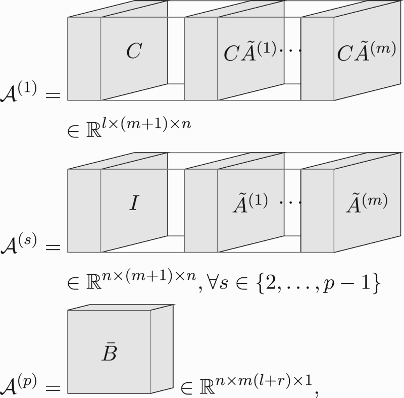
or equivalently, (29a) ${\mathcal{A}}^{\left(1\right)}\left(:,1,:\right)=C,$(29a) (29b) ${\mathcal{A}}^{\left(1\right)}\left(:,1+b,:\right)=C{\tilde{A}}^{\left(b\right)},\mathrm{\forall }b\in \{1,\dots ,m\},$(29b) (29c) ${\mathcal{A}}^{\left(s\right)}\left(:,1,:\right)=I_n,\mathrm{\forall }s\in \{2,\dots ,p-1\},$(29c) (29d) $\begin{array}{rl}{\mathcal{A}}^{\left(s\right)}\left(:,1+b,:\right)& ={\tilde{A}}^{\left(b\right)},\mathrm{\forall }b\in \{1,\dots ,m\},\\ & \mathrm{\forall }s\in \{2,\dots ,p-1\},\end{array}$(29d) (29e) ${\mathcal{A}}^{\left(p\right)}=\overline{B}.$(29e) Also, define the cores of the tensor network of the associated data matrix (per sample) in three-dimensional view as

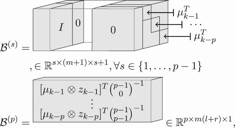
where $[{\mu }_{k-j}\otimes z_{k-j}{]}^T$ is a row vector, and equivalently, (30a) $\begin{array}{rl}{\mathcal{B}}_k^{\left(s\right)}\left(:,1,:\right)& =\left[\begin{array}{cc}{I}_s& 0\end{array}\right]\in {\mathbb{R}}^{s\times s+1}\\ & \mathrm{\forall }s\in \{1,\dots ,p-1\},\end{array}$(30a) (30b) $\begin{array}{rl}{\mathcal{B}}_k^{\left(s\right)}\left(:,1+b,:\right)& =\left[\begin{array}{ccccc}0& {\mu }_{k-1}^{\left(b\right)}& 0& \cdots & 0\\ 0& 0& {\mu }_{k-2}^{\left(b\right)}& \cdots & 0\\ ⋮& ⋮& ⋮& \ddots & ⋮\\ 0& 0& 0& 0& {\mu }_{k-s}^{\left(b\right)}\end{array}\right]\in {\mathbb{R}}^{s\times s+1}\\ & \mathrm{\forall }b\in \{1,\dots ,m\},\mathrm{\forall }s\in \{1,\dots ,p-1\},\end{array}$(30b) (30c) $\begin{array}{rl}{\mathcal{B}}_k^{\left(p\right)}& =\left[\begin{array}{c}[{\mu }_{k-1}\otimes z_{k-1}{]}^T{\left(\genfrac{}{}{0em}{}{p-1}{0}\right)}^{-1}\\ ⋮\\ [{\mu }_{k-p}\otimes z_{k-p}{]}^T{\left(\genfrac{}{}{0em}{}{p-1}{p-1}\right)}^{-1}\end{array}\right]\\ & \in {\mathbb{R}}^{p\times m(l+r)}.\end{array}$(30c) Notice that these cores have this specific sparse form, because Kronecker products of subsequent scheduling sequence samples appear in the data (see for example (11(11a) $P_{j|k}={\mu }_{k+j-1}\otimes \cdots \otimes {\mu }_k\otimes I_{l+r}\in {\mathbb{R}}^{(l+r)m^j\times (l+r)},$(11a) )). Proof of both decompositions follows through straightforward computations. The binomial coefficients in this last core divide entries of the full tensor by how many times they appear in the full tensor. These coefficients may give finite precision problems for $p\ge 58$. These cores are defined like this to keep the following data equation simple.

Using these two tensor networks, the predictor-based data equation can be recast as (31) $y_k\approx C{K}_{\left(p\right)}{Z}_k+e_k=⟨\mathbf{T},{\mathbf{Z}}_k⟩+e_k,$(31) where $⟨\ast ,\ast ⟩$ is the inner product (Definition 2.4), and $\mathbf{T}$ and ${\mathbf{Z}}_k$ are defined by their tensor networks: (32a) $\begin{array}{rl}\mathbf{T}& =g({\mathcal{A}}^{\left(1\right)},\dots ,{\mathcal{A}}^{\left(p\right)})\\ & \in {\mathbb{R}}^{l\times (m+1)\times \cdots \times (m+1)\times m(l+r)},\end{array}$(32a) (32b) $\begin{array}{rl}{\mathbf{Z}}_k& =g({\mathcal{B}}_k^{\left(1\right)},\dots ,{\mathcal{B}}_k^{\left(p\right)})\\ & \in {\mathbb{R}}^{1\times (m+1)\times \cdots \times (m+1)\times m(l+r)}.\end{array}$(32b) In detail, the full tensor $\mathbf{T}$ has $l(l+r)m(m+1{)}^{p-1}$ elements of which $l(l+r)\sum _{j=1}^p{m}^j$ (7(7) $q=(l+r)\sum _{j=1}^p{m}^j.$(7) ) are unique. The advantage of this recast is that $⟨\mathbf{T},{\mathbf{Z}}_k⟩$ can be computed ‘curse-of-dimensionality’-free in memory and computation using tensor networks (Definition 2.4).

In the next subsection, the state-revealing matrix is recast using tensor networks.

3.3. The state-revealing matrix

In this subsection, we present how the (estimate) state-revealing matrix (20(20) $R=\left[\begin{array}{cccc}C{L}_p& C{L}_{p-1}& \cdots & C{L}_1\\ 0& C{\tilde{A}}^{\left(1\right)}{L}_{p-1}& \cdots & C{\tilde{A}}^{\left(1\right)}{L}_1\\ ⋮& \ddots & \ddots & ⋮\\ 0& 0& & C{\left({\tilde{A}}^{\left(1\right)}\right)}^{f-1}{L}_1\end{array}\right]Z\in {\mathbb{R}}^{fl\times N-p},$(20) ) can be constructed from the (estimate) parameter tensor network (31(31) $y_k\approx C{K}_{\left(p\right)}{Z}_k+e_k=⟨\mathbf{T},{\mathbf{Z}}_k⟩+e_k,$(31) ) and the data sequence ‘curse-of-dimensionality’-free in memory and computation. Afterwards the (estimate) state sequence and state-space matrices can be obtained using Section 2.1.

Constructing the (estimate) state-revealing matrix R (20(20) $R=\left[\begin{array}{cccc}C{L}_p& C{L}_{p-1}& \cdots & C{L}_1\\ 0& C{\tilde{A}}^{\left(1\right)}{L}_{p-1}& \cdots & C{\tilde{A}}^{\left(1\right)}{L}_1\\ ⋮& \ddots & \ddots & ⋮\\ 0& 0& & C{\left({\tilde{A}}^{\left(1\right)}\right)}^{f-1}{L}_1\end{array}\right]Z\in {\mathbb{R}}^{fl\times N-p},$(20) ) in straightforward manner from the (estimate) LPV sub-Markov parameters and associated data matrix is problematic, because they both suffer from the ‘curse-of-dimensionality’. Therefore, we present how it can be constructed with tensor networks using the operator $h\left(\right)$ as (33a) $R=h({\mathcal{A}}^{\left(1\right)},\dots ,{\mathcal{A}}^{\left(p\right)},\mu ,z,f),$(33a) (33b) $R\left(\theta \right)=h\left({\mathcal{A}}^{\left(1\right)}\right(\theta ),\dots ,{\mathcal{A}}^{\left(p\right)}(\theta ),\mu ,z,f),$(33b) where R and ${\mathcal{A}}^{(\ast )}$ are defined in (20(20) $R=\left[\begin{array}{cccc}C{L}_p& C{L}_{p-1}& \cdots & C{L}_1\\ 0& C{\tilde{A}}^{\left(1\right)}{L}_{p-1}& \cdots & C{\tilde{A}}^{\left(1\right)}{L}_1\\ ⋮& \ddots & \ddots & ⋮\\ 0& 0& & C{\left({\tilde{A}}^{\left(1\right)}\right)}^{f-1}{L}_1\end{array}\right]Z\in {\mathbb{R}}^{fl\times N-p},$(20) ) and (29(29a) ${\mathcal{A}}^{\left(1\right)}\left(:,1,:\right)=C,$(29a) ), respectively, and the parametrisation is discussed in detail in the next section. Because the definition of $h\left(\right)$ is lengthy, its details are provided in Appendix 3. This equation allows computing the (estimate) state-revealing matrix ‘curse-of-dimensionality’-free in memory and computation.

In the next section, the proposed method is presented.

4. The proposed method

In this section, the proposed method is presented. The proposed refinement predictor-based method uses a tensor network parametrisation in order to obtain refined LPV state-space estimates ‘curse-of-dimensionality’-free in memory and computation. This can be as exploitation of the underlying tensor structure.

4.1. Parametrisation

A tensor network parametrisation of the LPV sub-Markov parameters is used by the proposed method. That is, the LPV sub-Markov parameter tensor (32(32a) $\begin{array}{rl}\mathbf{T}& =g({\mathcal{A}}^{\left(1\right)},\dots ,{\mathcal{A}}^{\left(p\right)})\\ & \in {\mathbb{R}}^{l\times (m+1)\times \cdots \times (m+1)\times m(l+r)},\end{array}$(32a) ) is parametrised as (34) $\mathbf{T}\left(\theta \right)=g\left({\mathcal{A}}^{\left(1\right)}\right({\theta }_1),\dots ,{\mathcal{A}}^{\left(p\right)}({\theta }_p\left)\right),$(34) with each core parametrised as black-box. Using the data equation (31(31) $y_k\approx C{K}_{\left(p\right)}{Z}_k+e_k=⟨\mathbf{T},{\mathbf{Z}}_k⟩+e_k,$(31) ), the model output can be described as (35) $y_k\left(\theta \right)=⟨\mathbf{T}\left(\theta \right),{\mathbf{Z}}_k⟩.$(35) Furthermore, the estimated state-revealing matrix (20(20) $R=\left[\begin{array}{cccc}C{L}_p& C{L}_{p-1}& \cdots & C{L}_1\\ 0& C{\tilde{A}}^{\left(1\right)}{L}_{p-1}& \cdots & C{\tilde{A}}^{\left(1\right)}{L}_1\\ ⋮& \ddots & \ddots & ⋮\\ 0& 0& & C{\left({\tilde{A}}^{\left(1\right)}\right)}^{f-1}{L}_1\end{array}\right]Z\in {\mathbb{R}}^{fl\times N-p},$(20) ) is (36) $R\left(\theta \right)=h\left({\mathcal{A}}^{\left(1\right)}\right({\theta }_1),\dots ,{\mathcal{A}}^{\left(p\right)}({\theta }_p),\mu ,z,f).$(36) Notice that the system order is generally not known, so the sizes of the cores will depend on the model order $\tilde{n}$ instead. We underline that this parametrisation is a free parametrisation and not canonical. Furthermore, the core and state estimates are modulo global state-coordinate transformation. In total there are $l(m+1)\tilde{n}+\left(\tilde{n}\right(m+1\left)\tilde{n}\right)(p-2)+\tilde{n}m(l+r)$ parameters to estimate. Notice that the number of LPV sub-Markov parameters is generally many times larger ($l(l+r)\sum _{j=1}^p{m}^j$ (7(7) $q=(l+r)\sum _{j=1}^p{m}^j.$(7) )). The parameter tensor $\mathbf{T}\left(\theta \right)$ has over-parametrisation: an LPV sub-Markov parameter can appear multiple times and each will be parametrised differently. The chosen parametrisation allows for well-known (tensor network) optimisation techniques.

The optimisation of these parameters is performed using ALS for tensor networks (Batselier et al., 2017; Oseledets, 2011). That is, we start with an initialisation of the cores and iteratively update them one-by-one. Every update boils down to solving a least squares problem (A.16(A16) $\overline{Y}={\overline{V}}^{\left(s\right)}\mathrm{vec}\left({\mathcal{A}}^{\left(s\right)}\right)+\overline{E},$(A16) ). Afterwards we make an orthogonalisation step in order to improve the conditioning of the next sub-problem. This orthogonalisation is also performed on the initialisation of the cores. We refer to Oseledets (2011), Batselier et al. (2017) and Chen, Batselier, Suykens, and Wong (2016) for this common step. For this orthogonalisation step, some assumptions are made on the sizes of the cores. Let ${\mathcal{A}}^{\left(s\right)}\left(\theta \right)$ be $\in {\mathbb{R}}^{a\times b\times c}$. Then, for $1\le s\le p-1$ we assume $ab\ge c$, and for $2\le s\le p$ we assume $bc\ge a$.

This optimisation approach enjoys some nice properties. Firstly, the optimisation has local linear convergence under some mild condition (Holtz, Rohwedder, & Schneider, 2012; Rohwedder & Uschmajew, 2013). Secondly, the condition number of the least squares problem of every sub-problem has upper bounds (Holtz et al., 2012). The latter result allows exchanging the assumption that each sub-problem is well-conditioned by the assumption that this upper bound holds (Holtz et al., 2012) and is finite. We show how to compute these bounds for our problem ‘curse-of-dimensionality’-free in memory and computation in Appendix 2.

In the next subsection, the algorithm of the proposed method is summarised.

4.2. Algorithm

Algorithm 4.1

The proposed method

Input: an initial estimate of the LPV state-space matrices, $\mu ,z,p,f,$ termination conditions

Output: a refined estimate of the LPV state-space matrices

1. Initialise the tensor network cores $\mathcal{A}\left(\theta \right)$ (34(34) $\mathbf{T}\left(\theta \right)=g\left({\mathcal{A}}^{\left(1\right)}\right({\theta }_1),\dots ,{\mathcal{A}}^{\left(p\right)}({\theta }_p\left)\right),$(34) ). This can be done using an initial estimate of the LPV state-space matrices and the formulas (29(29a) ${\mathcal{A}}^{\left(1\right)}\left(:,1,:\right)=C,$(29a) ). This initial estimate can be obtained from a (‘curse-of-dimensionality’-free in memory and computation) convex method, such as proposed by Gunes et al. (2016) and van Wingerden and Verhaegen (2009).

2. Compute the tensor network cores $\mathcal{B}$ of the data (30(30a) $\begin{array}{rl}{\mathcal{B}}_k^{\left(s\right)}\left(:,1,:\right)& =\left[\begin{array}{cc}{I}_s& 0\end{array}\right]\in {\mathbb{R}}^{s\times s+1}\\ & \mathrm{\forall }s\in \{1,\dots ,p-1\},\end{array}$(30a) ).

3. Optimise the tensor network cores $\mathcal{A}\left(\theta \right)$ using the tensor network ALS (Holtz et al., 2012) and Section 4.1 until the termination conditions(discussed in the next paragraph) are met. The sub-problems of this ALS are given in Appendix 1.

4. Use the estimate cores to compute the estimate state-revealing matrix using (33(33a) $R=h({\mathcal{A}}^{\left(1\right)},\dots ,{\mathcal{A}}^{\left(p\right)},\mu ,z,f),$(33a) ).

5. Use an SVD to obtain an estimate of the states as described in Section 2.1.

6. Solve two least squares problem to obtain a (refined) estimate of the LPV state-space matrices as described in van Wingerden and Verhaegen (2009).

The entire algorithm is ‘curse-of-dimensionality’-free in memory and computation. Some details on the algorithm are worth mentioning. Firstly notice that the initial estimate also provides a well-supported choice of the tensor network ranks, so these ranks can be kept fixed during optimisation. It is worth remarking that methods without fixed ranks exist such as the density matrix renormalisation group (DMRG) algorithm (White, 1992). Secondly, there are several ways to terminate theoptimisation. One option is to terminate when the residual changes less than $0.1\mathrm{\%}$ after updating all cores forward and backward. Another option is to terminate after a few such ‘sweeps’. We do not recommend a termination condition on the absolute residual itself for this application, as the LPV data equation (14(14) $y_{k+p}\approx C{K}_{\left(p\right)}{Z}_{k+p}+e_{k+p},$(14) ) can have non-negligible bias. Furthermore, in the simulations we will solve the least squares problem for every update with added Tikhonovregularisation. More specifically, instead of solving $\parallel \overline{Y}-{\overline{V}}^{\left(s\right)}\mathrm{vec}\left({\mathcal{A}}^{\left(s\right)}\right){\parallel }_F^2$ we solve $\parallel \overline{Y}-{\overline{V}}^{\left(s\right)}\mathrm{vec}\left({\mathcal{A}}^{\left(s\right)}\right){\parallel }_F^2+\lambda \parallel \mathrm{vec}\left({\mathcal{A}}^{\left(s\right)}\right){\parallel }_F^2$ where the definitions are given in Appendix 1. The tuning parameter λ is chosen using generalised cross validation (GCV) (Golub, Heath, & Wahba, 1979). Additionally, the computation cost of this algorithm scales favourably with the past window as a fifth power as $\mathcal{O}\left(p^5\right)$. This is dominated by the computation of the inner products in the ALS step. In the next section simulation results are presented to evaluate the performance of the proposed method.

5. Simulation results

In this section, we illustrate the performance of the proposed method with simulation results.

5.1. Simulation settings

In this section, the general simulation settings, constant over every case, are presented.

The following information is passed to the identification methods. All methods are passed the input, output and scheduling sequences. The model order is chosen equal to the system order. The future window in any SVD step is chosen equal to the past window. The evaluated methods are all global LPV identification methods for known arbitrary scheduling sequences. All cases generate data based on a finite-dimensional discrete affine state-space LPV system. Together with the proposed non-convex method, the convex LPV-PBSID${}_{opt}$ (kernel) method by van Wingerden and Verhaegen (2009), the non-convex predictor-based tensor regression (PBTR) method by Gunes et al. (2017) and the non-convex polynomial method by Verdult et al. (2003) are evaluated. More specifically, the LPV-PBSID${}_{opt}$ with its own Tikhonov regularisation and GCV, and the output error variant of the polynomial method (Verdult et al., 2003) is used. The proposed method is terminated after five sweeps. All the non-convex methods are initialised from the estimate of the convex method. Additionally, results are presented of the proposed method initialised in ‘random’ manner as follows. Firstly, m (3(3a) $x_{k+1}=\sum _{i=1}^m{\mu }_k^{\left(i\right)}\left(A^{\left(i\right)}{x}_k+B^{\left(i\right)}{u}_k+K^{\left(i\right)}{e}_k\right),$(3a) ) random, stable LTI systems with the chosen model order and matching input and output counts are generated. Secondly, these m LTI systems are combined in straightforward manner into an LPV system. Thirdly, this LPV system is regarded as an initial estimate. The matrix K is generated in the same way as B. These methods are or will soon be available with the PBSID toolbox (van Wingerden & Verhaegen, 2009). The convex method (Gunes et al., 2016) from previous work is not evaluated, because it is not related to the core contributions of the current paper. All results are based on 100 Monte Carlo simulations. For each Monte Carlo simulation, a different realisation of both the input and the innovation vector is used, while the scheduling sequence is kept the same.

The produced estimates are then scored using the Variance Accounted For (VAF) criterion on a validation data set. That is, fresh data not available to the methods is used which has different realisations of both the input and the innovation vector. The VAF for single-output systems is defined as follows (van Wingerden & Verhaegen, 2009): $\mathrm{VAF}({\overline{y}}_k,{\hat{y}}_k)=\max \left\{1-\frac{var({\overline{y}}_k-{\hat{y}}_k)}{var\left({\overline{y}}_k\right)},0\right\}100\mathrm{\%}.$ The variable ${\overline{y}}_k$ denotes the noise-free simulated output of the system, and similarly ${\hat{y}}_k$ denotes the noise-free (simulated) model output. The operator $var(\ast )$ returns the variance of its argument. If a non-convex refinement method returns an estimate with identification VAF 15% lower than that of its initialisation, then the refined estimate is rejected and substituted by the initialisation. Notice that this only involves identification data. Also notice that this does not prevent local minima, but only serves to reject known poor optimisation results. Finally, the computations are performed on an Intel i7 quad-core processor running at 2.7GHz with 8 GB RAM, and the computation times are provided. In the next subsections, we present several cases and the parameter counts.

5.2. Simulation results – Case 1

In this subsection, a case which relates to the flapping dynamics of a wind turbine is used to evaluate the performance of the proposed method and existing methods. This case has been used before in Felici, Van Wingerden, and Verhaegen (2007) and van Wingerden and Verhaegen (2009). Consider the following LPV state-space system (3(3a) $x_{k+1}=\sum _{i=1}^m{\mu }_k^{\left(i\right)}\left(A^{\left(i\right)}{x}_k+B^{\left(i\right)}{u}_k+K^{\left(i\right)}{e}_k\right),$(3a) ): $\begin{array}{rl}[A^{\left(1\right)},A^{\left(2\right)}]& =\left[\begin{array}{cc}0& 0.0734\\ -6.5229& 0.4997\end{array}\left|\begin{array}{cc}-0.0021& 0\\ -0.0138& 0.5196\end{array}\right.\right],\\ [B^{\left(1\right)},B^{\left(2\right)}]& =\left[\begin{array}{c}-0.7221\\ -9.6277\end{array}|\begin{array}{c}0\\ 0\end{array}\right],C=\left[\begin{array}{cc}1& 0\end{array}\right],\end{array}$ where D is zero and K is LPV. The matrix $K^{\left(i\right)}$ for $i=\{1,\dots ,m\}$ has been obtained from the discrete algebraic Ricatti equation (DARE) using $A^{\left(i\right)}$ and C and identity covariance of the concatenated process and measurement noise. The input $u_k$ is chosen as white noise with unit power and the innovation $e_k$ is also chosen as white noise with unit power. The past window is 6. The data size N is 200.

The system is evaluated at the affine scheduling sequence: ${\mu }_k^{\left(2\right)}=\cos \left(2\pi k\frac{10}{N}\right)/2+0.2.$ The results are shown in Table 1, Figures 1 and 2. The average computation times are 0.033, 15, 0.82, 10 and 9.4 s for, respectively, the LPV-PBSID${}_{opt}$, the PBTR, the polynomial and the proposed method (for pseudo-random and normal initialisation) per Monte Carlo simulation.

Figure 1. This figure shows a box-plot of the validation VAF of the 100 Monte Carlo simulations for five methods. The initialisation method is LPV-PBSID${}_{opt}$ (kernel), and the other four are refinement methods. The text ‘r.i.’ indicates random initialisation, as discussed in Section 5.1.

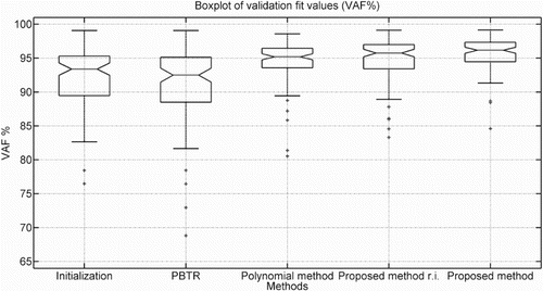
Figure 2. This figure shows how the validation VAF of the proposed method, averaged over the Monte Carlo simulations, is affected by the number of sweeps. The VAF at 0 sweeps performed is the initialisation. This sweep is defined in Section 4.1.

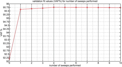
Table 1. Mean VAF for different methods for Case 1.

Method	VAF%
LPV-PBSID${}_{opt}$ (kernel)	92.2 $\pm 0.5$
PBTR	91.1 $\pm 0.6$
Polynomial method	94.6 $\pm 0.3$
Proposed method (r.i.)	94.8 $\pm 0.3$
Proposed method	95.8 $\pm 0.2$

Note: The text ‘r.i.’ indicates random initialisation, as discussed in Section 5.1.

From Table 1, Figures 1 and 2, it is visible that for this case the proposed method and the polynomial method can refine the initial estimates successfully. Two additional, minor results are that the proposed method may converge quickly and perform well for random initialisation.

5.3. Simulation results – Case 2

In this subsection, the proposed method is shown to work for a MIMO case with higher system order. Consider the following LPV state-space system (3(3a) $x_{k+1}=\sum _{i=1}^m{\mu }_k^{\left(i\right)}\left(A^{\left(i\right)}{x}_k+B^{\left(i\right)}{u}_k+K^{\left(i\right)}{e}_k\right),$(3a) ) with $\begin{array}{rl}{A}^{\left(1\right)}& =\left[\begin{array}{cccc}\frac{-15}{30}& 0& 0& 0\\ \frac{2}{30}& \frac{-17}{30}& \frac{-4}{30}& \frac{38}{30}\\ \frac{2}{30}& \frac{-2}{30}& \frac{-19}{30}& \frac{2}{30}\\ 0& 0& 0& \frac{21}{30}\end{array}\right],\\ A^{\left(2\right)}& =\left[\begin{array}{cccc}\frac{24}{30}& 0& 0& 0\\ \frac{9}{30}& \frac{15}{30}& \frac{-18}{30}& \frac{-18}{30}\\ \frac{9}{30}& \frac{-9}{30}& \frac{6}{30}& \frac{9}{30}\\ 0& 0& 0& \frac{-1}{30}\end{array}\right],\\ A^{\left(3\right)}& =\left[\begin{array}{cccc}0& 0& 0& 0\\ \frac{-2}{30}& \frac{2}{30}& \frac{4}{30}& \frac{-2}{30}\\ \frac{-2}{30}& \frac{2}{30}& \frac{4}{30}& \frac{-1}{30}\\ 0& 0& 0& 0\end{array}\right],\\ A^{\left(4\right)}& =\left[\begin{array}{cccc}0& 0& 0& 0\\ 0& 0& 0& \frac{6}{30}\\ 0& 0& 0& 0\\ 0& 0& 0& \frac{6}{30}\end{array}\right]\end{array}$ and $\begin{array}{rl}{B}^{\left(1\right)}& =\left[\begin{array}{cc}1& 0\\ 1& 0\\ 0& 1\\ 0& 1\end{array}\right],B^{\left(2\right)}=B^{\left(3\right)}=B^{\left(4\right)}=B^{\left(1\right)}/4,\\ C& =\left[\begin{array}{cccc}1& 0& 0& 0\\ 0& 1& 0& 0\\ 0& 0& 1& 0\end{array}\right],\end{array}$ where D is zero and K is LPV. The matrix $K^{\left(i\right)}$ for $i=\{1,\dots ,m\}$ has been obtained from the DARE using $A^{\left(i\right)}$ and C and identity covariance of the concatenated process and measurement noise. Every input signal is chosen as white noise with unit power and every innovation signal is chosen as white noise with half a unit power. The past window is 6. The data size N is 200.

The system is evaluated at the affine scheduling sequence: $\begin{array}{r}\begin{array}{rl}{\mu }_k^{\left(2\right)}& =\mathrm{sawtooth}\left(1+2\pi k\frac{1}{N}\right)/3+0.2\\ {\mu }_k^{\left(3\right)}& =\mathrm{sawtooth}\left(-1+2\pi k\frac{1}{N}/3.5+0.5\pi \right)\\ {\mu }_k^{\left(4\right)}& =\cos \left(2\pi k\frac{1}{N}/3\right)+0.2,\end{array}\end{array}$ where ‘sawtooth’ is a sawtooth wave function with peaks of $-1$ and 1. It is $-1$ when its argument is a multiple of $2\pi$. The results are shown in Table 2, Figures 3 and 4. The average computation times are 0.020 and 13  s for, respectively, the LPV-PBSID${}_{opt}$ method and the proposed method per Monte Carlo simulation.

Figure 3. This figure shows a box-plot of the validation VAF of the 100 Monte Carlo simulations for two methods. The initialisation method is LPV-PBSID${}_{opt}$ (kernel), and the refinement method is the proposed method.

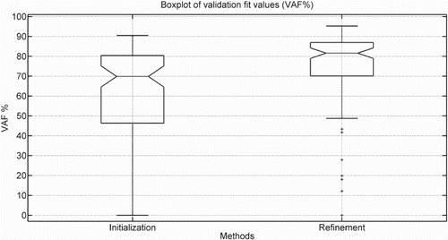
Figure 4. This figure shows a scatter-plot of the validation VAF of the 100 Monte Carlo simulations for two methods. The initialisation method is LPV-PBSID${}_{opt}$ (kernel), and the refinement method is the proposed method.

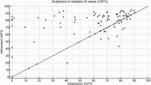
Table 2. Mean VAF for different methods for Case 2.

Method	Output channel	VAF%
	1	67.3 $\pm 2.9$
LPV-PBSID${}_{opt}$ (kernel)	2	54.5 $\pm 3.0$
	3	60.3 $\pm 3.3$
	1	79.7 $\pm 1.9$
Proposed method	2	73.9 $\pm 2.3$
	3	74.2 $\pm 2.4$

From the results of Table 2, Figure 3 and 4, it is visible that the proposed method can refine initial estimates for this case. We do remark that a few ‘refined’ estimates have decreased VAF, which is possible due to the two compared methods optimising different objective functions.

5.4. Parameter counts

For completeness, the parameter counts of several methods are presented in Table 3. The computational cost scaling is also briefly recapped. A more specific cost for the proposed method is given in Section 4.2.

Table 3. Comparison of the parameter counts for the (first) estimation step for model order equal to system order, and the computational cost scaling.

	Parameter count
Method	Formula	Case 1	Case 2	Computation cost scaling
LPV-PBSID${}_{opt}$ (primal)	$l(l+r){\displaystyle \sum _{j=1}^p{m}^j}$	252	81,900	c.o.d.
LPV-PBSID${}_{opt}$ (kernel)	lN	200	600	c.o.d.-free
PBTR	$nl+n(l+r)m$	50	412	c.o.d.
	$+n^{2}m(p-1)$
Polynomial method	$nl+nrm+n^{2}m$	14	108	c.o.d.-free
Proposed method	$l(m+1)n$	62	460	c.o.d.-free
	$+n^2(m+1)(p-2)$
	$+n(l+r)m$

Note: The abbreviation 'c.o.d.' stands for 'curse-of-dimensionality'.

This table shows that a straightforward black-box parametrisation, like LPV-PBSID${}_{opt}$ without kernels, results in a parameter count which scales exponentially. A more condense parametrisation can be obtained by using kernels (van Wingerden & Verhaegen, 2009) or a non-linear parametrisation. The parameter count of the proposed method is comparable with the one of PBTR and larger than the one of the polynomial method. The parameter counts for Case 2 show that the parameter counts of the evaluated methods are much smaller than the case for a straightforward approach.

6. Conclusions

In this paper, it was shown that the MIMO LPV identification problem with state-space matrices admits a tensor network description. That is, the LPV sub-Markov parameters, data and state-revealing matrix were condensely and exactly presented as tensor networks. Additionally, it was shown how to obtain the (estimate) state-revealing matrix directly from (estimate) tensor networks. These results provided a tensor network perspective on the MIMO LPV identification problem. Then, a refinement method was proposed which is ‘curse-of-dimensionality’-free in memory and computation and has conditioning guarantees. The performance of the proposed method was illustrated using simulation cases and additionally compared with existing methods.

Disclosure statement

No potential conflict of interest was reported by the authors.

ORCID

Bilal Gunes   http://orcid.org/0000-0002-2846-9519

Additional information

Funding

This work is funded and supported by the Design for Reliable Power Performance (D4REL) program, project code P91202.

Notes

1 Except the first and last one, as they are fixed at one (21(21) $\mathbf{T}\left(i_1,\dots ,i_d\right)={\mathcal{A}}^{\left(1\right)}\left(:,i_1,:\right){\mathcal{A}}^{\left(2\right)}\left(:,i_2,:\right)\dots {\mathcal{A}}^{\left(d\right)}\left(:,i_d,:\right),$(21) ).

Appendices

Appendix 1. Derivation of the least squares problem

The proposed method involves the optimisation of a tensor network using ALS. At every update of a tensor network core, a least squares problem must be solved. In this appendix, we derive that least squares problem.

Using the algorithm for the inner products of two tensor networks (Oseledets, 2011) and (29(29a) ${\mathcal{A}}^{\left(1\right)}\left(:,1,:\right)=C,$(29a) ), (30(30a) $\begin{array}{rl}{\mathcal{B}}_k^{\left(s\right)}\left(:,1,:\right)& =\left[\begin{array}{cc}{I}_s& 0\end{array}\right]\in {\mathbb{R}}^{s\times s+1}\\ & \mathrm{\forall }s\in \{1,\dots ,p-1\},\end{array}$(30a) ), we can state that (A1) $⟨\mathbf{T},{\mathbf{Z}}_k⟩=\prod _{s=1}^{s=p}\sum _{i_s=1}^{n_s}{\mathcal{A}}^{\left(s\right)}\left(:,i_s,:\right)\otimes {\mathcal{B}}_k^{\left(s\right)}\left(:,i_s,:\right),$(A1) where $n_s$ is (A2) $n_s=m+1\mathrm{for}s\le p-1,\mathrm{otherwise}m(l+r)$(A2) and the operator $\prod$ is defined as (A3) $\prod _{i=1}^d{M}_i=M_1{M}_2\dots M_d.$(A3) Then, we can isolate the sth core: (A4) $⟨\mathbf{T},{\mathbf{Z}}_k⟩=V_{-,k}^{\left(s\right)}\left(\sum _{i_s=1}^{n_s}{\mathcal{A}}^{\left(s\right)}\left(:,i_s,:\right)\otimes {\mathcal{B}}_k^{\left(s\right)}\left(:,i_s,:\right)\right)V_{+,k}^{\left(s\right)},$(A4) where ${\mathcal{A}}^{\left(s\right)}\in {\mathbb{R}}^{\overline{m}\times n_s\times \overline{n}}$, ${\mathcal{B}}_k^{\left(s\right)}\in {\mathbb{R}}^{\overline{p}\times n_s\times \overline{q}}$, and (A5) $\begin{array}{rl}{V}_{-,k}^{\left(s\right)}& =I_{\overline{m}\overline{p}}\mathrm{for}s=1,\\ & \prod _{t=1}^{t=s-1}\sum _{i_t=1}^{n_t}{\mathcal{A}}^{\left(t\right)}\left(:,i_t,:\right)\otimes {\mathcal{B}}_k^{\left(t\right)}\left(:,i_t,:\right)\mathrm{otherwise},\end{array}$(A5) and (A6) $\begin{array}{rl}{V}_{+,k}^{\left(s\right)}& =I_{\overline{n}\overline{q}}\mathrm{for}s=p,\\ & \prod _{t=s+1}^{t=p}\sum _{i_t=1}^{n_t}{\mathcal{A}}^{\left(t\right)}\left(:,i_t,:\right)\otimes {\mathcal{B}}_k^{\left(t\right)}\left(:,i_t,:\right)\mathrm{otherwise}.\end{array}$(A6) Using the Kronecker algebra trick in Batselier et al. (2017), we can rewrite (A7) $\begin{array}{rl}⟨\mathbf{T},{\mathbf{Z}}_k⟩& =\left((V_{+,k}^{\left(s\right)}{)}^T\otimes V_{-,k}^{\left(s\right)}\right)\\ & \times \sum _{i_s=1}^{n_s}\mathrm{vec}\left({\mathcal{A}}^{\left(s\right)}\left(:,i_s,:\right)\otimes {\mathcal{B}}_k^{\left(s\right)}\left(:,i_s,:\right)\right),\end{array}$(A7) where we additionally pulled the summer out of the vectorisation operator $\mathrm{vec}(\ast )$. Next we use the following equivalence (Turkington, 2013). For a matrix M of size $\overline{m}$-by-$\overline{n}$ and a matrix N of size $\overline{p}$-by-$\overline{q}$: (A8) $\mathrm{vec}(M\otimes N)=(I_{\overline{n}}\otimes {\overline{K}}_{\overline{q}\overline{m}}\otimes I_{\overline{p}})(I_{\overline{m}\overline{n}}\otimes \mathrm{vec}(N\left)\right)\mathrm{vec}\left(M\right),$(A8) where the matrix $\overline{K}$ is defined such that (A9) ${\overline{K}}_{\overline{m}\overline{n}}\mathrm{vec}\left(M\right)=\mathrm{vec}\left(M^T\right).$(A9) Now we can fill in (A10) $\begin{array}{rl}M& ={\mathcal{A}}^{\left(s\right)}\left(:,i_s,:\right),\\ N& ={\mathcal{B}}_k^{\left(s\right)}\left(:,i_s,:\right)\end{array}$(A10) to obtain (A11) $\begin{array}{rl}⟨\mathbf{T},{\mathbf{Z}}_k⟩& =\left((V_{+,k}^{\left(s\right)}{)}^T\otimes V_{-,k}^{\left(s\right)}\right)(I_{\overline{n}}\otimes {\overline{K}}_{\overline{q}\overline{m}}\otimes I_{\overline{p}})\sum _{i_s=1}^{n_s}\\ & \times (I_{\overline{m}\overline{n}}\otimes \mathrm{vec}({\mathcal{B}}_k^{\left(s\right)}\left(:,i_s,:\right)\left)\mathrm{vec}\right({\mathcal{A}}^{\left(s\right)}\left(:,i_s,:\right)).\end{array}$(A11) Notice that the sizes are constant over $i_s$. Next we can rewrite without summation: (A12) $\begin{array}{rl}⟨\mathbf{T},{\mathbf{Z}}_k⟩& =\left((V_{+,k}^{\left(s\right)}{)}^T\otimes V_{-,k}^{\left(s\right)}\right)(I_{\overline{n}}\otimes {\overline{K}}_{\overline{q}\overline{m}}\otimes I_{\overline{p}})\\ & \times [I_{\overline{m}\overline{n}}\otimes \mathrm{vec}({\mathcal{B}}_k^{\left(s\right)}\left(:,1,:\right))\dots ]\\ & \times \left[\begin{array}{c}\mathrm{vec}\left({\mathcal{A}}^{\left(s\right)}\right(:,1,:\left)\right)\\ ⋮\\ \mathrm{vec}\left({\mathcal{A}}^{\left(s\right)}\right(:,n_s,:\left)\right)\end{array}\right].\end{array}$(A12) We can further simplify this equation by reorganising the right-most matrix into $\mathrm{vec}\left({\mathcal{A}}^{\left(s\right)}\right)$ as follows. Define the matrix ${\overline{V}}_k^{\left(s\right)}$ in pseudo-code: (A13) $\begin{array}{rl}{\overline{V}}_k^{\left(s\right)}& =\mathrm{reshape}\left(\mathrm{permute}\right(\mathrm{reshape}(\\ & \times \left((V_{+,k}^{\left(s\right)}{)}^T\otimes V_{-,k}^{\left(s\right)}\right)(I_{\overline{n}}\otimes {\overline{K}}_{\overline{q}\overline{m}}\otimes I_{\overline{p}})\\ & \times \left[I_{\overline{m}\overline{n}}\otimes \mathrm{vec}\left({\mathcal{B}}_k^{\left(s\right)}\right(:,1,:\left)\right)\dots \right],\\ & [l,\overline{m},n_s,\overline{n}]),[1,2,4,3\left]\right),[l,\overline{m}{n}_s\overline{n}]),\end{array}$(A13) where the two functions are defined as follows. The ‘reshape’ function changes the size of the dimensions of its first argument as specified in its second argument. The ordering of the elements is not changed. The ‘permute’ function changes the indexing of its first argument as specified in its second argument. Then, we obtain (using (31(31) $y_k\approx C{K}_{\left(p\right)}{Z}_k+e_k=⟨\mathbf{T},{\mathbf{Z}}_k⟩+e_k,$(31) )): (A14) $y_k\approx ⟨\mathbf{T},{\mathbf{Z}}_k⟩+e_k={\overline{V}}_k^{\left(s\right)}\mathrm{vec}\left({\mathcal{A}}^{\left(s\right)}\right)+e_k.$(A14) We can stack this over all samples. Define (A15) $\begin{array}{rl}{\overline{V}}^{\left(s\right)}& =\left[\begin{array}{c}{\overline{V}}_{p+1}^{\left(s\right)}\\ ⋮\\ {\overline{V}}_N^{\left(s\right)}\end{array}\right]\in {\mathbb{R}}^{l(N-p)\times \overline{m}{n}_s\overline{n}},\overline{Y}=\left[\begin{array}{c}{y}_{p+1}\\ ⋮\\ y_N\end{array}\right],\\ \overline{E}& =\left[\begin{array}{c}{e}_{p+1}\\ ⋮\\ e_N\end{array}\right]\in {\mathbb{R}}^{l(N-p)},\end{array}$(A15) such that (A16) $\overline{Y}={\overline{V}}^{\left(s\right)}\mathrm{vec}\left({\mathcal{A}}^{\left(s\right)}\right)+\overline{E},$(A16) where it is assumed that $l(N-p)$ is greater than or equal to the number of elements of each ${\mathcal{A}}^{\left(s\right)}$. Additionally, upper bounds are derived on the condition number of ${\overline{V}}^{\left(s\right)}$ in Appendix 2. This is the least squares problem that has to be solved when updating a core.

Appendix 2. The condition guarantee

The proposed method uses ALS to optimise its tensor network cores. This involves solving a number of sub-problems (A.16(A16) $\overline{Y}={\overline{V}}^{\left(s\right)}\mathrm{vec}\left({\mathcal{A}}^{\left(s\right)}\right)+\overline{E},$(A16) ), whose conditioning depends on the condition number of ${\overline{V}}^{\left(s\right)}$. In this appendix, we derive an upper bound on this condition number using Holtz et al. (2012). Notice that this property is in part due to the orthogonalisation steps of tensor network ALS. Additionally, we provide a means to compute it ‘curse-of-dimensionality’-free in memory and computation.

Firstly, define the condition number of a matrix as the ratio of the largest singular value of that matrix to the smallest singular value. If the smallest singular value is zero, then the condition number is by convention infinite. Let ‘cond$\left(\right)$’ be an operator whose output is the condition number of its argument.

Define using (31(31) $y_k\approx C{K}_{\left(p\right)}{Z}_k+e_k=⟨\mathbf{T},{\mathbf{Z}}_k⟩+e_k,$(31) ): (A17) $\check{Y}=\left[\begin{array}{c}{y}_{p+1}^T\\ ⋮\\ y_N^T\end{array}\right],\check{E}=\left[\begin{array}{c}{e}_{p+1}^T\\ ⋮\\ e_N^T\end{array}\right],\check{\mathbf{Z}}=\left[\begin{array}{c}\mathrm{vec}({\mathbf{Z}}_{p+1}{)}^T\\ ⋮\\ \mathrm{vec}({\mathbf{Z}}_N{)}^T\end{array}\right],$(A17) such that we can rewrite (31(31) $y_k\approx C{K}_{\left(p\right)}{Z}_k+e_k=⟨\mathbf{T},{\mathbf{Z}}_k⟩+e_k,$(31) ) as (A18) $\check{Y}\approx (C{K}_{\left(p\right)}Z{)}^T+\check{E}=\check{\mathbf{Z}}({\mathbf{T}}_{⟨1⟩}{)}^T+\check{E}.$(A18) Additionally, we assume that the chosen initialisation of the tensor network cores results in all ${\overline{V}}^{\left(s\right)}$ (A.16(A16) $\overline{Y}={\overline{V}}^{\left(s\right)}\mathrm{vec}\left({\mathcal{A}}^{\left(s\right)}\right)+\overline{E},$(A16) ) being invertible at the start of the optimisation. Then, using the results of Holtz et al. (2012), we can now state that the condition number of each ${\overline{V}}^{\left(s\right)}$ (A.16(A16) $\overline{Y}={\overline{V}}^{\left(s\right)}\mathrm{vec}\left({\mathcal{A}}^{\left(s\right)}\right)+\overline{E},$(A16) ) is upper bounded by the condition number of the matrix $\check{\mathbf{Z}}$.

Next, we provide means to compute the latter condition number ‘curse-of-dimensionality’-free in memory and computation using tensor trains. Notice that $\check{\mathbf{Z}}$ suffers from the ‘curse-of-dimensionality’, such that the computation of its condition number is problematic. However, since $\check{\mathbf{Z}}$ only has N−p rows, the following trick can be applied. For any wide matrix M, $\text{cond}\left[M\right]=\text{cond}\left[\right(M{M}^T{)}^{1/2}]$ holds. Notice that $M{M}^T$ is smaller than the wide M. Hence, we use that (A19) $\text{cond}\left[\check{\mathbf{Z}}\right]=\text{cond}\left[\right(\check{\mathbf{Z}}{\check{\mathbf{Z}}}^T{)}^{1/2}],$(A19) where the size of $(\check{\mathbf{Z}}{\check{\mathbf{Z}}}^T{)}^{1/2}$ is only N−p-by-N−p. Hence, $\text{cond}\left[\right(\check{\mathbf{Z}}{\check{\mathbf{Z}}}^T{)}^{1/2}]$ can be computed if $\left(\check{\mathbf{Z}}{\check{\mathbf{Z}}}^T\right)$ is available. In other words, the size and square root do not induce any ‘curse-of-dimensionality’, such that the problem reduces to computing the following equation ‘curse-of-dimensionality’-free in memory and computation. This reduced problem can be tackled using tensor trains. Using (A.17(A17) $\check{Y}=\left[\begin{array}{c}{y}_{p+1}^T\\ ⋮\\ y_N^T\end{array}\right],\check{E}=\left[\begin{array}{c}{e}_{p+1}^T\\ ⋮\\ e_N^T\end{array}\right],\check{\mathbf{Z}}=\left[\begin{array}{c}\mathrm{vec}({\mathbf{Z}}_{p+1}{)}^T\\ ⋮\\ \mathrm{vec}({\mathbf{Z}}_N{)}^T\end{array}\right],$(A17) ) (A20) $\left[\check{\mathbf{Z}}{\check{\mathbf{Z}}}^T\right]\left(i,j\right)=\mathrm{vec}\left({\mathbf{Z}}_{p+i}{)}^T\mathrm{vec}\right({\mathbf{Z}}_{p+j}),$(A20) or equivalently (A21) $\left[\check{\mathbf{Z}}{\check{\mathbf{Z}}}^T\right]\left(i,j\right)=⟨{\mathbf{Z}}_{p+i},{\mathbf{Z}}_{p+j}⟩$(A21) which is an inner product of two tensor trains (Definition 2.4). This inner product and, with it, the upper bound on the condition number can be computed ‘curse-of-dimensionality’-free in memory and computation.

Appendix 3. The operator for the state-revealing matrix

In Section 2.1 it has been discussed how the estimate (LPV sub-Markov) parameters can be used to obtain an estimate of the state sequence. This is done by constructing the estimate state-revealing matrix $R\left(\theta \right)$ and taking its SVD. In this appendix, we show how to obtain this matrix from the estimate tensor networks ‘curse-of-dimensionality’-free in memory and computation.

Recall that R has been defined as (20(20) $R=\left[\begin{array}{cccc}C{L}_p& C{L}_{p-1}& \cdots & C{L}_1\\ 0& C{\tilde{A}}^{\left(1\right)}{L}_{p-1}& \cdots & C{\tilde{A}}^{\left(1\right)}{L}_1\\ ⋮& \ddots & \ddots & ⋮\\ 0& 0& & C{\left({\tilde{A}}^{\left(1\right)}\right)}^{f-1}{L}_1\end{array}\right]Z\in {\mathbb{R}}^{fl\times N-p},$(20) ): (A22) $R=\left[\begin{array}{cccc}C{L}_p& C{L}_{p-1}& \cdots & C{L}_1\\ 0& C{\tilde{A}}^{\left(1\right)}{L}_{p-1}& \cdots & C{\tilde{A}}^{\left(1\right)}{L}_1\\ ⋮& \ddots & \ddots & ⋮\\ 0& 0& & C{\left({\tilde{A}}^{\left(1\right)}\right)}^{f-1}{L}_1\end{array}\right]Z\in {\mathbb{R}}^{fl\times N-p}.$(A22) Notice that both matrices of the product suffer from the ‘curse-of-dimensionality’. However, we can avoid this problem by using the tenor networks as in (33(33a) $R=h({\mathcal{A}}^{\left(1\right)},\dots ,{\mathcal{A}}^{\left(p\right)},\mu ,z,f),$(33a) ) (A23a) $R=h({\mathcal{A}}^{\left(1\right)},\dots ,{\mathcal{A}}^{\left(p\right)},\mu ,z,f),$(A23a) (A23b) $R\left(\theta \right)=h\left({\mathcal{A}}^{\left(1\right)}\right(\theta ),\dots ,{\mathcal{A}}^{\left(p\right)}(\theta ),\mu ,z,f),$(A23b) where some operator $h(\ast )$ is used which is ‘curse-of-dimensionality’-free in memory and computation.

This operator is non-trivial, because of the following reason. The rows of R involve subsets of the LPV sub-Markov parameters and the relation of these subsets to the tensor network decomposition is complex. Firstly, the LPV sub-Markov parameters appear multiple times in the parameter tensor and require averaging. Secondly, the tensor network cores contain identity matrices which add further ambiguity. The remainder of this appendix provides details on the functionality of this operator. The operator is presented formally in Algorithm A.2.

The operator $h(\ast )$ consists of several loops. The major loop is over the outputs. That is, we split the full problem into l single-output sub-problems. Then, we solve each sub-problem individually and merge the results. How we split and merge is presented in full detail in Algorithm A.2. How we solve each sub-problem will be introduced next. In the remainder of this appendix we consider one such sub-problem with output number o for clarity.

For each such sub-problem, we compute the state-revealing matrix (20(20) $R=\left[\begin{array}{cccc}C{L}_p& C{L}_{p-1}& \cdots & C{L}_1\\ 0& C{\tilde{A}}^{\left(1\right)}{L}_{p-1}& \cdots & C{\tilde{A}}^{\left(1\right)}{L}_1\\ ⋮& \ddots & \ddots & ⋮\\ 0& 0& & C{\left({\tilde{A}}^{\left(1\right)}\right)}^{f-1}{L}_1\end{array}\right]Z\in {\mathbb{R}}^{fl\times N-p},$(20) ) with C replaced by $C_o=C(o,:)$. The top row of this matrix is $C_o{K}_{\left(p\right)}Z$ and can be computed efficiently using inner products of tensor networks (31(31) $y_k\approx C{K}_{\left(p\right)}{Z}_k+e_k=⟨\mathbf{T},{\mathbf{Z}}_k⟩+e_k,$(31) ), where C is substituted by $C_o$. The other rows are more involved.

The difficulty of the other rows is that we do not have a single inner product, because these rows involve only subsets of the LPV sub-Markov parameters. Namely, row number t only involves LPV sub-Markov parameters whose product begins with $C_o({\tilde{A}}^{\left(1\right)}{)}^{t-1}$ (20(20) $R=\left[\begin{array}{cccc}C{L}_p& C{L}_{p-1}& \cdots & C{L}_1\\ 0& C{\tilde{A}}^{\left(1\right)}{L}_{p-1}& \cdots & C{\tilde{A}}^{\left(1\right)}{L}_1\\ ⋮& \ddots & \ddots & ⋮\\ 0& 0& & C{\left({\tilde{A}}^{\left(1\right)}\right)}^{f-1}{L}_1\end{array}\right]Z\in {\mathbb{R}}^{fl\times N-p},$(20) ). Therefore, we compute these rows in two parts. The first part relates to the required begin of the product, and the second part relates to the ‘free’ part.

Before presenting the computation, we first provide insight into how LPV sub-Markov parameters appear multiple times in the parameter tensor and how to deal with this. The reason LPV sub-Markov parameters appear multiple times in the parameter tensor is that they can be constructed in different ways from the tensor train cores. For example consider the (1,2,1)th and (2,1,1)th entry of the estimate parameter tensor for three cores: (A24) $\begin{array}{rl}\mathbf{T}(1,2,1)\left(\theta \right)& =\left[C_o\right]\left({\theta }_1\right)\left[{\tilde{A}}^{\left(1\right)}\right]\left({\theta }_2\right)\left[B^{\left(1\right)}\right]\left({\theta }_3\right),\\ \mathbf{T}(2,1,1)\left(\theta \right)& =\left[C_o{\tilde{A}}^{\left(1\right)}\right]\left({\theta }_1\right)\left[I\right]\left({\theta }_2\right)\left[B^{\left(1\right)}\right]\left({\theta }_3\right).\end{array}$(A24) Both relate to the same LPV sub-Markov parameter. To be exact, LPV sub-Markov parameters with c many ${\tilde{A}}^{(\ast )}$'s appear $\left(\genfrac{}{}{0em}{}{p-1}{c}\right)$ times. This phenomenon poses a problem, as we have several estimates of the same LPV sub-Markov parameter. It turns out that discarding all but one estimate is not viable, because it changes the model output. However, averaging estimates does not change the model output and removes the ambiguity. This is possible because the estimates are multiplied with the same data during the computation of the model output. We will explain later in this subsection how to perform this averaging efficiently.

First we define the matrix S in order to store all possible ways of fixing the cores to obtain the subset of LPV sub-Markov parameters relevant to one row of the state-revealing matrix. Let the number of cores we fix be δ. Then, we need to fix δ cores, of which t−1 cores to ${\tilde{A}}^{\left(1\right)}$ and the rest as I. The last core we have to fix as ${\tilde{A}}^{\left(1\right)}$, for reasons we will explain later in this subsection. This becomes a pick t−2 cores out of $\delta -1$ cores problem. This can be done in $\left(\genfrac{}{}{0em}{}{\delta -1}{t-2}\right)$ ways. For every possible way, we put a row in S where the sth element of that row is a 1 if core s is fixed at ${\tilde{A}}^{\left(1\right)}$ and a 0 otherwise for s is one to δ. We summarise this algorithm:

Algorithm A.1

$S=f_S(\delta ,t)$

For every possible way of picking t−2 cores out of $\delta -1$ cores, put a row in S, where the sth element of that row is a 1 if core s is picked and a 0 otherwise. Let the δth element of that row be 1. This results in a $\left(\genfrac{}{}{0em}{}{\delta -1}{t-2}\right)$-by-δ matrix.

We illustrate the result of the algorithm with an example: (A25) $f_S(\delta =4,t=4)=\left[\begin{array}{cccc}0& 1& 1& 1\\ 1& 0& 1& 1\\ 1& 1& 0& 1\end{array}\right].$(A25)

In this paragraph, we discuss why we need δ in the computations. The LPV sub-Markov parameters related to the tth row all start with $C({\tilde{A}}^{\left(1\right)}{)}^{t-1}$, and we can isolate these by fixing cores. This we can do by fixing the first t−1 cores as $C{\tilde{A}}^{\left(1\right)}$ and ${\tilde{A}}^{\left(1\right)}$. The remaining cores are ‘free’. We can also do this while fixing more cores, by fixing some at I. That can also leave a number of cores ‘free’. Therefore, to capture all estimates of the same LPV sub-Markov parameter, we have to consider $\delta =t-1$ to p−1. Additionally, to avoid counting estimates double, we let the last fixed core always be fixed at ${\tilde{A}}^{\left(1\right)}$. Now we return to how to perform the computations of the operator $h(\ast )$.

The first part of the computation relates to the fixed cores. The fixed cores are simply matrices. More specifically, they are slices of the cores corresponding to either I or ${\tilde{A}}^{\left(1\right)}$. They form a series of matrix products. This product returns a row vector, as we consider one output at a time. We define this product as $\overline{L}$.

The second part of the computation relates to the ‘free’ cores. Notice that for the top row we had no fixed cores and directly used a tensor network inner product. Here we again use inner products. We form a reduced tensor network from the free cores. To match this smaller size tensor network in size, we also define a reduced data tensor network. This tensor network can simply be computed using (30(30a) $\begin{array}{rl}{\mathcal{B}}_k^{\left(s\right)}\left(:,1,:\right)& =\left[\begin{array}{cc}{I}_s& 0\end{array}\right]\in {\mathbb{R}}^{s\times s+1}\\ & \mathrm{\forall }s\in \{1,\dots ,p-1\},\end{array}$(30a) ) with p substituted by $p-\delta$, and the following change.

Additionally, we have to change the duplication correction factors (30(30a) $\begin{array}{rl}{\mathcal{B}}_k^{\left(s\right)}\left(:,1,:\right)& =\left[\begin{array}{cc}{I}_s& 0\end{array}\right]\in {\mathbb{R}}^{s\times s+1}\\ & \mathrm{\forall }s\in \{1,\dots ,p-1\},\end{array}$(30a) ) to account for the effect of δ not being just zero. Therefore, we define the matrix $D_r$: (A26) $D_r=\left[\begin{array}{ccc}\left(\genfrac{}{}{0em}{}{p-(t-1)}{1}\right){\left(\genfrac{}{}{0em}{}{p-\delta -1}{0}\right)}^{-1}& \cdots & 0\\ ⋮& \ddots & ⋮\\ 0& \cdots & \left(\genfrac{}{}{0em}{}{p-(t-1)}{p-\delta }\right){\left(\genfrac{}{}{0em}{}{p-\delta -1}{p-\delta -1}\right)}^{-1}\end{array}\right],$(A26) such that changing the last data tensor network core as (A27) ${\check{\mathcal{B}}}_k^{(p-\delta )}=D_r{\check{\mathcal{B}}}_k^{(p-\delta )}$(A27) ensures the correct duplication correction factors for the computation of the state-revealing matrix. Notice that ${\check{\mathcal{B}}}_k^{(p-\delta )}$ is a matrix. This then forms the tensor network of the reduced data tensor.

Then, we combine these computations to obtain the state-revealing matrix of the sub-problem. Namely, we post-multiply L with the inner product of the reduced parameter and reduced data tensor networks. This is done over several loops, over: the sample, row, δ and rows of S. We remark that the operator $R(\ast )$ is ‘curse-of-dimensionality’-free in memory and computation. Next we summarise the computation of the operator $h(\ast )$ in the following algorithm in pseudo-code.

Algorithm A.2

The operator $h(\ast )$

Input: (estimate) ${\mathcal{A}}^{\left(1\right)},\dots ,{\mathcal{A}}^{\left(p\right)},\mu ,z,f$

Output: (estimate) state-revealing matrix R

1. R $=\overline{0}\in {\mathbb{R}}^{fl\times N-p}$

2. for o=1 to l do

3.  ${\overline{\mathcal{A}}}_o^{\left(1\right)}={\mathcal{A}}^{\left(1\right)}(o,:,:)$

4.  $R^{\left(o\right)}=\overline{h}({\overline{\mathcal{A}}}^{\left(1\right)},{\mathcal{A}}^{\left(2\right)},\dots ,{\mathcal{A}}^{\left(p\right)},\mu ,z,f)$

    using Algorithm A.3

5.  v=o:l:fl

6.  $R(v,:)=R^{\left(o\right)}$

7. end for

Algorithm A.3

The operator $\overline{h}(\ast )$

Input: (estimate) ${\overline{\mathcal{A}}}^{\left(1\right)},{\mathcal{A}}^{\left(2\right)},\dots ,{\mathcal{A}}^{\left(p\right)},\mu ,z,f$

Output: (estimate) state-revealing matrix $R^{\left(o\right)}$

1. $R^{\left(o\right)}=\overline{0}\in {\mathbb{R}}^{f\times N-p}$

2. for k=p+1 to N do

3.  $R\left(1,k-p\right)=⟨\mathbf{T},{\mathbf{Z}}_k⟩$ using (31(31) $y_k\approx C{K}_{\left(p\right)}{Z}_k+e_k=⟨\mathbf{T},{\mathbf{Z}}_k⟩+e_k,$(31) )

4.  for row number t=2 to f do

5.   for fixed cores number $\delta =t-1$ to p−1 do

6.    $S=f_S(\delta ,t)\in {\mathbb{R}}^{\overline{c}\times \delta }$ using Algorithm A.1

7.    for c=1 to $\overline{c}$

8.     $\overline{L}={\mathcal{A}}^{\left(1\right)}\left(:,1+S\left(c,1\right),:\right)$

9.     for s=2 to δ

10.      $\overline{L}=\overline{L}{\mathcal{A}}^{\left(s\right)}\left(:,1+S\left(c,s\right),:\right)$

11.     end for

12.     $\check{\mathbf{T}}=g({\mathcal{A}}^{(1+\delta )},\dots ,{\mathcal{A}}^{\left(p\right)})$ using (22(22) $\mathbf{T}=g({\mathcal{A}}^{\left(1\right)},\dots ,{\mathcal{A}}^{\left(d\right)}),$(22) )

13.     Compute ${\check{\mathcal{B}}}_k^{\left(1\right)}$ to ${\check{\mathcal{B}}}_k^{(p-\delta )}$ using (30(30a) $\begin{array}{rl}{\mathcal{B}}_k^{\left(s\right)}\left(:,1,:\right)& =\left[\begin{array}{cc}{I}_s& 0\end{array}\right]\in {\mathbb{R}}^{s\times s+1}\\ & \mathrm{\forall }s\in \{1,\dots ,p-1\},\end{array}$(30a) )

        with p substituted by $p-\delta$

14.     ${\check{\mathcal{B}}}_k^{(p-fixno)}=D_r{\check{\mathcal{B}}}_k^{(p-\delta )}$ using (A.26(A26) $D_r=\left[\begin{array}{ccc}\left(\genfrac{}{}{0em}{}{p-(t-1)}{1}\right){\left(\genfrac{}{}{0em}{}{p-\delta -1}{0}\right)}^{-1}& \cdots & 0\\ ⋮& \ddots & ⋮\\ 0& \cdots & \left(\genfrac{}{}{0em}{}{p-(t-1)}{p-\delta }\right){\left(\genfrac{}{}{0em}{}{p-\delta -1}{p-\delta -1}\right)}^{-1}\end{array}\right],$(A26) )

15.     ${\check{\mathbf{Z}}}_k=g({\check{\mathcal{B}}}_k^{\left(1\right)},\dots ,{\check{\mathcal{B}}}_k^{(p-\delta )})$ using (22(22) $\mathbf{T}=g({\mathcal{A}}^{\left(1\right)},\dots ,{\mathcal{A}}^{\left(d\right)}),$(22) )

16.     $R^{\left(o\right)}\left(t,k-p\right)=R^{\left(o\right)}\left(t,k-p\right)+$

        $\overline{L}⟨\check{\mathbf{T}},{\check{\mathbf{Z}}}_k⟩/\overline{c}$

17.    end for

18.   end for

19.  end for

20. end for

References

- Balas, G. J. (2002). Linear, parameter-varying control and its application to aerospace systems. ICAS Congress proceedings, Toronto, Canada (pp. 541.1–541.9).
- Batselier, K., Chen, Z., & Wong, N. (2017). Tensor network alternating linear scheme for MIMO Volterra system identification. Automatica, 84, 26–35. doi: 10.1016/j.automatica.2017.06.033
- Bianchi, F. D., Mantz, R. J., & Christiansen, C. F. (2005). Gain scheduling control of variable-speed wind energy conversion systems using quasi-LPV models. Control Engineering Practice, 13(2), 247–255. doi: 10.1016/j.conengprac.2004.03.006
- Brewer, J. (1978). Kronecker products and matrix calculus in system theory. IEEE Transactions on Circuits and Systems, 25(9), 772–781. doi: 10.1109/TCS.1978.1084534
- Chen Z., Batselier K., Suykens J. A., & Wong N. (2016). Parallelized tensor train learning for polynomial pattern classification. arXiv preprint arXiv:1612.06505.
- Chiuso, A. (2007). The role of vector autoregressive modeling in predictor-based subspace identification. Automatica, 43(6), 1034–1048. doi: 10.1016/j.automatica.2006.12.009
- Cox, P., & Tóth, R. (2016). Alternative form of predictor based identification of LPV-SS models with innovation noise. 2016 IEEE 55th conference on decision and control (CDC), Las Vegas, United States of America (pp. 1223–1228).
- De Caigny, J., Camino, J. F., & Swevers, J. (2009). Interpolating model identification for SISO linear parameter-varying systems. Mechanical Systems and Signal Processing, 23(8), 2395–2417. doi: 10.1016/j.ymssp.2009.04.007
- De Silva, V., & Lim, L.-H. (2008). Tensor rank and the ill-posedness of the best low-rank approximation problem. SIAM Journal on Matrix Analysis and Applications, 30(3), 1084–1127. doi: 10.1137/06066518X
- Felici, F., Van Wingerden, J.-W., & Verhaegen, M. (2007). Subspace identification of MIMO LPV systems using a periodic scheduling sequence. Automatica, 43(10), 1684–1697. doi: 10.1016/j.automatica.2007.02.027
- Gebraad, P. M., van Wingerden, J.-W., Fleming, P. A., & Wright, A. D. (2011). LPV subspace identification of the edgewise vibrational dynamics of a wind turbine rotor. 2011 IEEE International Conference on Control Applications (CCA), Denver, United States of America (pp. 37–42).
- Gebraad, P. M., van Wingerden, J.-W., Fleming, P. A., & Wright, A. D. (2013). LPV identification of wind turbine rotor vibrational dynamics using periodic disturbance basis functions. IEEE Transactions on Control Systems Technology, 21(4), 1183–1190. doi: 10.1109/TCST.2013.2257775
- Giarré, L., Bauso, D., Falugi, P., & Bamieh, B. (2006). LPV model identification for gain scheduling control: An application to rotating stall and surge control problem. Control Engineering Practice, 14(4), 351–361. doi: 10.1016/j.conengprac.2005.01.013
- Golub, G. H., Heath, M., & Wahba, G. (1979). Generalized cross-validation as a method for choosing a good ridge parameter. Technometrics, 21(2), 215–223. doi: 10.1080/00401706.1979.10489751
- Gunes B., van Wingerden J.-W., & Verhaegen M. (2016). Tensor nuclear norm LPV subspace identification. Transactions on Automatic Control, conditionally accepted.
- Gunes, B., van Wingerden, J.-W., & Verhaegen, M. (2017). Predictor-based tensor regression (PBTR) for LPV subspace identification. Automatica, 79, 235–243. doi: 10.1016/j.automatica.2017.01.039
- Håstad, J. (1990). Tensor rank is NP-complete. Journal of Algorithms, 11(4), 644–654. doi: 10.1016/0196-6774(90)90014-6
- Holtz, S., Rohwedder, T., & Schneider, R. (2012). The alternating linear scheme for tensor optimization in the tensor train format. SIAM Journal on Scientific Computing, 34(2), A683–A713. doi: 10.1137/100818893
- Knudsen, T. (2001). Consistency analysis of subspace identification methods based on a linear regression approach. Automatica, 37(1), 81–89. doi: 10.1016/S0005-1098(00)00125-4
- Larimore, W. E., & Buchholz, M. (2012). ADAPT-LPV software for identification of nonlinear parameter-varying systems. IFAC Proceedings Volumes, 45(16), 1820–1825. doi: 10.3182/20120711-3-BE-2027.00418
- Laurain, V., Gilson, M., Tóth, R., & Garnier, H. (2010). Refined instrumental variable methods for identification of LPV Box–Jenkins models. Automatica, 46(6), 959–967. doi: 10.1016/j.automatica.2010.02.026
- Oseledets, I. V. (2011). Tensor-train decomposition. SIAM Journal on Scientific Computing, 33(5), 2295–2317. doi: 10.1137/090752286
- Remmlinger, J., Buchholz, M., & Dietmayer, K. (2013). Identification of a bilinear and parameter-varying model for lithium-ion batteries by subspace methods. 2013 American control conference (ACC), Washington, DC, United States of America (pp. 2268–2273).
- Rohwedder, T., & Uschmajew, A. (2013). On local convergence of alternating schemes for optimization of convex problems in the tensor train format. SIAM Journal on Numerical Analysis, 51(2), 1134–1162. doi: 10.1137/110857520
- Scherer, C. W. (2001). LPV control and full block multipliers. Automatica, 37(3), 361–375. doi: 10.1016/S0005-1098(00)00176-X
- Shamma, J. S. (2012). An overview of LPV systems. In J. Mohammadpour, & C. W. Scherer (Eds.), Control of linear parameter varying systems with applications (pp. 3–26). Boston, MA: Springer.
- Tóth, R. (2010). Modeling and identification of linear parameter-varying systems (Vol. 403). Springer.
- Tóth, R., Abbas, H. S., & Werner, H. (2012). On the state-space realization of LPV input–output models: Practical approaches. IEEE Transactions on Control Systems Technology, 20(1), 139–153.
- Turkington, D. A. (2013). Generalized vectorization, cross-products, and matrix calculus. Cambridge: Cambridge University Press.
- van der Maas, R., van der Maas, A., & Oomen, T. (2015). Accurate frequency response function identification of LPV systems: A 2D local parametric modeling approach. 2015 IEEE 54th annual conference on decision and control (CDC), Osaka, Japan (pp. 1465–1470).
- van der Veen, G., van Wingerden, J.-W., Bergamasco, M., Lovera, M., & Verhaegen, M. (2013). Closed-loop subspace identification methods: An overview. IET Control Theory & Applications, 7(10), 1339–1358. doi: 10.1049/iet-cta.2012.0653
- van Wingerden, J.-W., & Verhaegen, M. (2009). Subspace identification of bilinear and LPV systems for open- and closed-loop data. Automatica, 45(2), 372–381. doi: 10.1016/j.automatica.2008.08.015
- Verdult V., Bergboer N., & Verhaegen M. (2003). Identification of fully parameterized linear and nonlinear state-space systems by projected gradient search. Proceedings of the 13th IFAC symposium on system identification, Rotterdam.
- Wassink, M. G., van de Wal, M., Scherer, C., & Bosgra, O. (2005). LPV control for a wafer stage: Beyond the theoretical solution. Control Engineering Practice, 13(2), 231–245. doi: 10.1016/j.conengprac.2004.03.008
- White, S. R. (1992). Density matrix formulation for quantum renormalization groups. Physical Review Letters, 69(19), 2863. doi: 10.1103/PhysRevLett.69.2863