Robust load frequency control of nonlinear power networks^*

* Preliminary results appeared in Trip, Cucuzzella, Ferrara, and De Persis (2017).

ABSTRACT

This paper proposes a decentralised second-order sliding mode (SOSM) control strategy for load frequency control (LFC) in power networks, regulating the frequency and maintaining the net inter-area power flows at their scheduled values. The considered power network is partitioned into control areas, where each area is modelled by an equivalent generator including second-order turbine-governor dynamics, and where the areas are nonlinearly coupled through the power flows. Asymptotic convergence to the desired state is established by constraining the state of the power network on a suitably designed sliding manifold. This manifold is designed relying on stability considerations made on the basis of an incremental energy (storage) function. Simulation results confirm the effectiveness of the proposed control approach.

KEYWORDS:

• Sliding mode control
• decentralised control
• stability of nonlinear systems
• power systems stability

1. Introduction

To operate the power network successfully, the total generation should match the total load demand and associated system losses. It is however common that over time mismatches occur, resulting in a deviation of the system frequency from its nominal value and in power flows between the areas that differ from their scheduled exchanges. A weighted combination of the deviations in the frequency and in the tie-line power flows is generally called the ‘Area Control Error’ (ACE). Reducing this error is achieved by the so-called load frequency control (LFC) or automatic generation control (AGC), where an appropriate control scheme changes governor setpoints to compensate for local load changes and to maintain the scheduled tie-line power flows (Kundur, Balu, & Lauby, 1994).

Since the power network can be regarded as one of the most important infrastructures, improving LFC received a considerable amount of attention from various research communities (Ibraheem, Kumar, & Kothari, 2005; Pandey, Mohanty, & Kishor, 2013). Particularly, due to the increasing share of renewable energy sources, it is unsure if the existing implementations are still adequate (Apostolopoulou, Domínguez-García, & Sauer, 2016). To cope with the increasing uncertainties affecting a control area and to improve the controllers performance, advanced control techniques have been proposed to redesign the conventional control schemes, such as passivity-based control (Pogromsky, Fradkov, & Hill, 1996), model predictive control (Ersdal, Imsland, & Uhlen, 2016), adaptive control (Zribi, Al-Rashed, & Alrifai, 2005) and fuzzy control (Chang & Fu, 1997).

In this work, we propose a new control strategy based on the sliding mode (SM) control methodology, which is a well-known robust control approach, especially useful to control systems subject to modelling uncertainties and external disturbances (Edwards & Spurgen, 1998; Utkin, 1992). Since the power network is typically subject to modelling uncertainties and external disturbances (Furtat & Fradkov, 2015), there are indeed various SM-based approaches to improve the conventional LFC schemes (Dong, 2016; Mi, Fu, Wang, & Wang, 2013; Trip, Cucuzzella, Persis, van der Schaft, & Ferrara, 2018), possibly together with fuzzy logic (Ha, 1998), genetic algorithms (Vrdoljak, Perić, & Petrović, 2010), disturbances observers (Mi et al., 2016) and linear matrix inequalities (LMI) based control techniques (Prasad, Purwar, & Kishor, 2015).

1.1. Main contributions

Although the use of SMs in LFC has received a considerable amount of attention, the solution proposed in this work and the associated stability analysis differ substantially from the aforementioned works. Particularly, we notice that a common assumption in the literature is that the coupling between the control areas is linear. Instead, we consider a more realistic nonlinear coupling between the control areas, induced by the nonlinear power flow equations, which poses new challenges in the design of the sliding manifold. To the best of our knowledge, we are not aware of existing controllers for nonlinear power networks (including second-order turbine-governor dynamics) that provably achieve frequency regulation while maintaining the scheduled tie-line power flows. We summarise the main contributions of this work as follows:

1. The considered nonlinear power network model is more general than commonly considered in the analytical studies of LFC schemes. In this paper, we adopt the model of a power network partitioned into control areas, having an arbitrarily complex and meshed topology. Besides including the nonlinear coupling between the areas, we model the generation side by an equivalent generator including second-order turbine-governor dynamics. Particularly, the appearance of nonlinear power flows in combination with the second-order turbine-governor dynamics is challenging as it requires the development of a new nonlinear storage function for the stability analysis (Trip & De Persis, 2018).

2. SM control typically generates discontinuous control inputs that could lead to an undesired chattering effect (Utkin, 2016; Ventura & Fridman, 2016) and/or damage the system actuator. In this work, we argue that the use of higher order SM schemes are beneficial to LFC, as they result in a continuous control input, avoiding to possibly damage the (mechanical) turbine governor. Particularly, we focus on the suboptimal second-order sliding mode (SSOSM) control algorithm proposed in Bartolini, Ferrara, and Usai (1998a), and explicitly design a decentralised controller. Moreover, the convergence to the sliding manifold is obtained neither measuring the power demand, nor using load observers.

3. When the power network is constrained to the designed sliding manifold, the convergence towards the desired state is established relying on a Barbashin–Krasovskii–LaSalle invariance principle, and a new incremental storage function, composed of a commonly used incremental energy function (Trip, Bürger, & De Persis, 2016) and additional cross-terms. Particularly, the design of a nonlinear sliding function is inspired by the proposed nonlinear incremental storage function. A case study shows the effectiveness of the proposed controller and demonstrates that, besides the immediate application to LFC, the combined use of sliding mode control and other nonlinear control techniques can provide new insights and control strategies.

1.2. Outline

The present paper is organised as follows: In Section 2, the network model is introduced. In Section 3, the considered LFC problem is formulated. The proposed controller is described in Section 4. The stability of the controlled power network is studied in Section 5. Simulation results are reported and discussed in Section 6, while some conclusions are finally gathered in Section 7.

1.3. Notation

Let $\mathbf{0}$ be the vector of all zeros of suitable dimension and let ${\mathbf{1}}_n$ be the vector containing all ones of length n. The ith element of vector x is denoted by $x_i$. A constant signal is denoted by $x^{\ast }$. A steady-state solution to system $\dot{x}=\zeta \left(x\right)$, is denoted by $\overline{x}$, i.e. $\mathbf{0}=\zeta \left(\overline{x}\right)$. In case the argument of a function is clear from the context, we occasionally write $\zeta \left(x\right)$ as ζ. Let $A\in {\mathbb{R}}^{n\times n}$ be a matrix. In case A is a positive definite (positive semi-definite) matrix, we write $A\succ 0$ ($A⪰0$). The sign function is defined as follows (Shtessel, Edwards, Fridman, & Levant, 2014): (1) $\mathrm{sgn}\left(x\right):=\{\begin{array}{ll}-1& \mathrm{if}x<0,\\ 1& \mathrm{if}x>0,\end{array}$(1) and $\mathrm{sgn}\left(0\right)\in [-1,1]$.

2. Nonlinear power network model

In this section, the dynamic model of a power network partitioned into control areas is presented. The dynamic behaviour of a single control area is described by an aggregated load and an equivalent thermal power plant with a non-reheat turbine, which is commonly represented by second-order turbine-governor dynamics. A block diagram of the considered system with two control areas is represented in Figure 1 (see also Table 1 for the description of the used symbols). Consequently, the dynamic equations of the ith area are the following: (2) $\begin{array}{rl}{\dot{\delta }}_i& ={\omega }_i^b\\ T_{pi}{\dot{\omega }}_i^b& =-({\omega }_i^b-{\omega }^{\ast })+K_{pi}{P}_{ti}-K_{pi}{P}_{di}\\ & -K_{pi}\sum _{j\in {\mathcal{A}}_i}\frac{V_i^{\ast }{V}_j^{\ast }}{X_{ij}}\sin ({\delta }_i-{\delta }_j),\end{array}$(2) where ${\mathcal{A}}_i$ is the set of control areas connected to the ith area by transmission lines. Note that we assume that the network is lossless, which is generally valid in high-voltage transmission networks where the line resistance is negligible. Moreover, $P_{ti}$ in (2(2) $\begin{array}{rl}{\dot{\delta }}_i& ={\omega }_i^b\\ T_{pi}{\dot{\omega }}_i^b& =-({\omega }_i^b-{\omega }^{\ast })+K_{pi}{P}_{ti}-K_{pi}{P}_{di}\\ & -K_{pi}\sum _{j\in {\mathcal{A}}_i}\frac{V_i^{\ast }{V}_j^{\ast }}{X_{ij}}\sin ({\delta }_i-{\delta }_j),\end{array}$(2) ) is the power generated by the ith plant, and it can be expressed as the output of the following second-order dynamical system that describes the behaviour of both the governor and the turbine: (3) $\begin{array}{rl}{T}_{gi}{\dot{P}}_{gi}& =-\frac{1}{R_i}({\omega }_i^b-{\omega }^{\ast })-P_{gi}+u_i\\ T_{ti}{\dot{P}}_{ti}& =-P_{ti}+P_{gi}.\end{array}$(3) In this paper, we aim at the design of a continuous control input $u_i$ to achieve frequency regulation and to maintain the power flows at their desired (scheduled) values. These control objectives will be made explicit in the next section. First, we suggest a compact notation for the overall power network that is useful for the upcoming discussions.

Figure 1. Block diagram of two interconnected control areas.

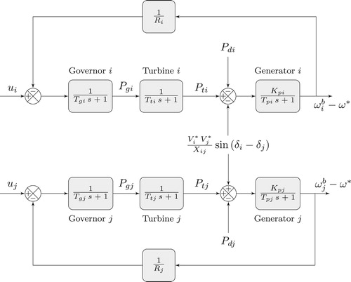
Table 1. Description of the used symbols.

Symbol	Description
${\delta }_i$	Voltage angle
${\omega }_i^b$	Frequency
${\omega }_i$	Frequency deviation
$P_{ti}$	Turbine output power
$P_{gi}$	Governor output
${\omega }^{\ast }$	Nominal frequency
$T_{pi}$	Time constant of the control area
$T_{ti}$	Time constant of the turbine
$T_{gi}$	Time constant of the governor
$K_{pi}$	Gain of the control area
$R_i$	Speed regulation coefficient
$V_i^{\ast }$	Constant voltage
$X_{ij}$	Line reactance
$u_i$	Control input
$P_{di}$	Unknown power demand

The considered power network consists of n interconnected control areas, of which the topology is represented by a connected and undirected graph $\mathcal{G}=(\mathcal{V},\mathcal{E})$, where the nodes $\mathcal{V}=\{1,\dots ,n\}$, represent the control areas and the edges $\mathcal{E}\subset \mathcal{V}\times \mathcal{V}=\{1,\dots ,m\}$, represent the transmission lines connecting the areas. The topology can be described by its corresponding incidence matrix $\mathcal{B}\in {\mathbb{R}}^{n\times m}$. Then, by arbitrarily labelling the ends of edge k with a ‘+’ and a ‘−’, one has that ${\mathcal{B}}_{ik}=\{\begin{array}{ll}+1& \mathrm{if}i\mathrm{is}\mathrm{the}\mathrm{positive}\mathrm{end}\mathrm{of}k\\ -1& \mathrm{if}i\mathrm{is}\mathrm{the}\mathrm{negative}\mathrm{end}\mathrm{of}k\\ 0& \mathrm{otherwise}.\end{array}$ The dynamics of the overall power network can now be compactly written for all areas $i\in \mathcal{V}$ as (4) $\begin{array}{rl}\dot{\eta }& ={\mathcal{B}}^{\mathrm{T}}\omega \\ T_p{K}_p^{-1}\dot{\omega }& =-K_p^{-1}\omega +P_t-P_d-\mathcal{B}\mathrm{\Gamma }\sin \left(\eta \right)\\ T_g{\dot{P}}_g& =-R^{-1}\omega -P_g+u\\ T_t{\dot{P}}_t& =-P_t+P_g,\end{array}$(4) where $\omega ={\omega }^b-{\omega }^{\ast }{\mathbf{1}}_n\in {\mathbb{R}}^n$ is the frequency deviation, $P_t\in {\mathbb{R}}^n$, $P_g\in {\mathbb{R}}^n$, $\mathrm{\Gamma }=\mathrm{diag}\{{\mathrm{\Gamma }}_1,\dots ,{\mathrm{\Gamma }}_m\}$, with ${\mathrm{\Gamma }}_k=V_i^{\ast }{V}_j^{\ast }/X_{ij}$, where line k connects areas i and j, $\sin \left(\eta \right)=(\sin ({\eta }_1),\dots ,\sin ({\eta }_m){)}^{\mathrm{T}}$, $P_d\in {\mathbb{R}}^n$ and $u\in {\mathbb{R}}^n$. Note furthermore that we introduced the variable $\eta ={\mathcal{B}}^{\mathrm{T}}\delta \in {\mathbb{R}}^m$, where element ${\eta }_k$ is the difference in voltage angles across line k between areas i and j. Matrices $T_p,T_t,T_g,K_p,R$ are positive definite $n\times n$ diagonal matrices, e.g. $K_p=\mathrm{diag}\{K_{p1},\dots ,K_{pn}\}$.

3. Problem formulation

Before focussing on the controller design, we formulate the two main objectives of LFC (automatic generation control). The first objective is concerned with the stead-state frequency deviation $\overline{\omega }$, i.e. with $\underset{t\to \mathrm{\infty }}{lim}\omega \left(t\right)$.

Objective 1

Frequency regulation

(5) $\underset{t\to \mathrm{\infty }}{lim}\omega \left(t\right)=\overline{\omega }=\mathbf{0}.$(5)

Let $(\mathcal{B}{P}_f^{\ast }{)}_i$ denote the total desired power flow exchanged by control area $i\in \mathcal{V}$, $P_f^{\ast }$ being an external reference signal. The second objective is to maintain the scheduled net power flows between the control areas.

Objective 2

Maintaining scheduled net power flows

(6) $\underset{t\to \mathrm{\infty }}{lim}\mathcal{B}\mathrm{\Gamma }\sin \left(\eta \right(t\left)\right)=\mathcal{B}\mathrm{\Gamma }\sin \left(\overline{\eta }\right)=\mathcal{B}{P}_f^{\ast }.$(6)

In case the power network does not contain cycles, Objective 2 is equivalent to $\underset{t\to \mathrm{\infty }}{lim}\mathrm{\Gamma }\sin \left(\eta \right(t\left)\right)=P_f^{\ast }$, such that the power flow on every line is regulated towards its desired value (see also Remark 5.2 in Section 5). To be able to achieve Objectives 1 and 2, we make the following assumption on the feasibility of the control problem:

Assumption 3.1

Feasibility

For a given constant $P_d^{\ast },$ there exist a constant input $\overline{u}$ and state $(\overline{\omega }=\mathbf{0},\overline{\eta },{\overline{P}}_g,{\overline{P}}_t)$ that satisfies (7) $\begin{array}{rl}\mathbf{0}& ={\mathcal{B}}^{\mathrm{T}}\mathbf{0}\\ \mathbf{0}& =-K_p^{-1}\mathbf{0}+{\overline{P}}_t-P_d^{\ast }-\mathcal{B}\mathrm{\Gamma }\sin \left(\overline{\eta }\right)\\ \mathbf{0}& =-R^{-1}\mathbf{0}-{\overline{P}}_g+\overline{u}\\ \mathbf{0}& =-{\overline{P}}_t+{\overline{P}}_g,\end{array}$(7) where $\mathcal{B}\mathrm{\Gamma }\sin \left(\overline{\eta }\right)=\mathcal{B}{P}_f^{\ast }$.

To increase the practical applicability, we furthermore desire the controllers to be decentralised and to be able to provide a continuous control input, avoiding to damage the turbine governor. We are now in a position to formulate the control problem:

Control Problem 1

Let Assumption 3.1 hold. Given system (4(4) $\begin{array}{rl}\dot{\eta }& ={\mathcal{B}}^{\mathrm{T}}\omega \\ T_p{K}_p^{-1}\dot{\omega }& =-K_p^{-1}\omega +P_t-P_d-\mathcal{B}\mathrm{\Gamma }\sin \left(\eta \right)\\ T_g{\dot{P}}_g& =-R^{-1}\omega -P_g+u\\ T_t{\dot{P}}_t& =-P_t+P_g,\end{array}$(4) ), design a decentralised control scheme, providing a continuous control input u, capable of guaranteeing that the controlled system is asymptotically stable with zero steady-state frequency deviation (Objective 1), maintaining, at the steady state, the scheduled (net) power flows (Objective 2).

4. The proposed robust solution

In this section, a decentralised SOSM control scheme is proposed to solve the aforementioned control problem. In this work, we focus on the well-established SSOSM controller proposed in Bartolini et al. (1998a) and apply it to the power network augmented with an additional state variable $\theta \in {\mathbb{R}}^n$ with dynamics (8) $T_{\theta }\dot{\phantom{a}}\theta =-\theta +P_t,$(8) that will provide additional freedom to shape the transient behaviour. To facilitate the upcoming discussion, we recall for convenience the following definitions that are essential to sliding mode control:

Definition 4.1

Sliding function

Consider system (9) $\dot{x}=\zeta (x,u),$(9) with state $x\in {\mathbb{R}}^n$, and input $u\in {\mathbb{R}}^m$. The sliding function $\sigma \left(x\right):{\mathbb{R}}^n\to {\mathbb{R}}^m$ is a sufficiently smooth output function of system (9(9) $\dot{x}=\zeta (x,u),$(9) ).

Definition 4.2

r-sliding manifold

The r-sliding manifold¹ is given by (10) $\{x\in {\mathbb{R}}^n,u\in {\mathbb{R}}^m:\sigma =L_{\zeta }\sigma =\cdots =L_{\zeta }^{(r-1)}\sigma =\mathbf{0}\},$(10) where $L_{\zeta }^{(r-1)}\sigma \left(x\right)$ is the $(r-1)$th order Lie derivative of $\sigma \left(x\right)$ along the vector field $\zeta (x,u)$. With a slight abuse of notation we also write $L_{\zeta }\sigma \left(x\right)=\dot{\sigma }\left(x\right)$, and $L_{\zeta }^{\left(2\right)}\sigma \left(x\right)=\ddot{\sigma }\left(x\right)$.

Definition 4.3

r-order sliding mode (controller)

An r-order sliding mode is enforced from $t=T_r\ge 0$, when, starting from an initial condition, the state of (9(9) $\dot{x}=\zeta (x,u),$(9) ) reaches the r-sliding manifold, and remains there for all $t\ge T_r$. The order of a sliding mode controller that enforces an r-order sliding mode is equal to r.

Bearing in mind the definitions above, we propose for the system at hand, the sliding function $\sigma (\omega ,P_t,P_g,\theta ,\eta ):{\mathbb{R}}^{4n+m}\to {\mathbb{R}}^n$ given by (11) $\sigma =M_1\omega +M_2{P}_t+M_3{P}_g+M_4\theta +M_5\mathcal{B}(\mathrm{\Gamma }\sin (\eta )-P_f^{\ast }),$(11) where $M_1,\dots ,M_5$ are constant $n\times n$ diagonal matrices, suitable selected in order to assign the dynamics of the augmented system on the manifold $\sigma =\mathbf{0}$. The sliding function (11(11) $\sigma =M_1\omega +M_2{P}_t+M_3{P}_g+M_4\theta +M_5\mathcal{B}(\mathrm{\Gamma }\sin (\eta )-P_f^{\ast }),$(11) ) is stated in an ad-hoc manner to facilitate the discussion on the controller design. Nevertheless, the choice of (11(11) $\sigma =M_1\omega +M_2{P}_t+M_3{P}_g+M_4\theta +M_5\mathcal{B}(\mathrm{\Gamma }\sin (\eta )-P_f^{\ast }),$(11) ) is inspired by the stability analysis in Section 5. Particularly, the permitted values for $M_1,\dots ,M_5$ follow directly from the stability analysis, and we provide explicit values for these matrices in Assumption 5.1 in the next section.

Regarding the sliding function (11(11) $\sigma =M_1\omega +M_2{P}_t+M_3{P}_g+M_4\theta +M_5\mathcal{B}(\mathrm{\Gamma }\sin (\eta )-P_f^{\ast }),$(11) ) as the output function² of system (4(4) $\begin{array}{rl}\dot{\eta }& ={\mathcal{B}}^{\mathrm{T}}\omega \\ T_p{K}_p^{-1}\dot{\omega }& =-K_p^{-1}\omega +P_t-P_d-\mathcal{B}\mathrm{\Gamma }\sin \left(\eta \right)\\ T_g{\dot{P}}_g& =-R^{-1}\omega -P_g+u\\ T_t{\dot{P}}_t& =-P_t+P_g,\end{array}$(4) ), (8(8) $T_{\theta }\dot{\phantom{a}}\theta =-\theta +P_t,$(8) ), the relative degree³ is one. This implies that a first-order sliding mode controller can be naturally applied in order to make the state of the controlled system reach, in a finite time, the manifold $\sigma =\mathbf{0}$. However, a sliding mode controller typically generates a fast switching discontinuous control input that could lead to an undesired chattering effect (Utkin, 2016; Ventura & Fridman, 2016) and/or damage the actuator. As a consequence, it is important to provide a continuous control input u to the governor. To obtain a continuous input u, we adopt the procedure suggested in Bartolini et al. (1998a), yielding for system (4(4) $\begin{array}{rl}\dot{\eta }& ={\mathcal{B}}^{\mathrm{T}}\omega \\ T_p{K}_p^{-1}\dot{\omega }& =-K_p^{-1}\omega +P_t-P_d-\mathcal{B}\mathrm{\Gamma }\sin \left(\eta \right)\\ T_g{\dot{P}}_g& =-R^{-1}\omega -P_g+u\\ T_t{\dot{P}}_t& =-P_t+P_g,\end{array}$(4) ) augmented with (8(8) $T_{\theta }\dot{\phantom{a}}\theta =-\theta +P_t,$(8) ): (12) $\begin{array}{rl}\dot{\eta }& ={\mathcal{B}}^{\mathrm{T}}\omega \\ T_p{K}_p^{-1}\dot{\omega }& =-K_p^{-1}\omega +P_t-P_d-\mathcal{B}\mathrm{\Gamma }\sin \left(\eta \right)\\ T_g{\dot{P}}_g& =-R^{-1}\omega -P_g+u\\ T_t{\dot{P}}_t& =-P_t+P_g\\ T_{\theta }\dot{\phantom{a}}\theta & =-\theta +P_t\\ \dot{u}& =w,\end{array}$(12) where w is the new (discontinuous) input generated by a sliding mode controller discussed below. Note that indeed the input signal to the governor, $u\left(t\right)={\int }_0^{t}w\left(\tau \right)\mathrm{d}\tau$, is continuous, since, as will we show later, the input w is piecewise constant. Furthermore, a consequence of the previous procedure is that the system relative degree (with respect to the new control input w) is now two, and we need to rely on a second-order sliding mode control strategy to attain the sliding manifold $\sigma =\dot{\sigma }=\mathbf{0}$ in a finite time (Levant, 2003). To make the controller design explicit, we introduce two auxiliary variables ${\xi }_1=\sigma$ and ${\xi }_2=\dot{\sigma }$ and define the so-called auxiliary system as follows: (13) $\begin{array}{rl}{\dot{\xi }}_1& ={\xi }_2\\ {\dot{\xi }}_2& =\phi +Gw\\ \dot{u}& =w,\end{array}$(13) where ${\xi }_2$ is not measurable as it depends, e.g. on the unknown power demand $P_d$. Bearing in mind (11(11) $\sigma =M_1\omega +M_2{P}_t+M_3{P}_g+M_4\theta +M_5\mathcal{B}(\mathrm{\Gamma }\sin (\eta )-P_f^{\ast }),$(11) ) and that $\ddot{\sigma }=\phi +Gw$, it follows that $\phi \in {\mathbb{R}}^n$ and $G\in {\mathbb{R}}^{n\times n}$ are given by (14) $\begin{array}{rl}\phi & =(M_1{T}_p^{-2}+M_3{R}^{-1}{T}_p^{-1}{T}_g^{-1}-M_2{R}^{-1}{T}_t^{-1}{T}_g^{-1}\\ & +M_3{R}^{-1}{T}_g^{-2})\omega -(M_1{K}_p{T}_p^{-2}+M_3{K}_p{R}^{-1}{T}_p^{-1}{T}_g^{-1}\\ & +M_1{K}_p{T}_p^{-1}{T}_t^{-1}-M_2{T}_t^{-2}+M_4{T}_t^{-1}{T}_{\theta }^{-1}+M_4{T}_{\theta }^{-2})P_t\\ & +(M_1{K}_p{T}_p^{-1}{T}_t^{-1}-M_2{T}_t^{-2}-M_2{T}_t^{-1}{T}_g^{-1}+M_3{T}_g^{-2}\\ & +M_4{T}_t^{-1}{T}_{\theta }^{-1})P_g+(M_2{T}_t^{-1}-M_3{T}_g^{-1})T_g^{-1}u\\ & +(M_1{T}_p^{-1}+M_3{R}^{-1}{T}_g^{-1})(K_p{T}_p^{-1}{P}_d+K_p{T}_p^{-1}\mathcal{B}\mathrm{\Gamma }\sin (\eta \left)\right)\\ & -M_1{K}_p{T}_p^{-1}({\dot{P}}_d+\mathcal{B}\mathrm{\Gamma }\frac{\mathrm{d}}{\mathrm{d}t}\sin (\eta \left)\right)\\ & +M_5\mathcal{B}\mathrm{\Gamma }\frac{{\mathrm{d}}^2}{\mathrm{d}t}\sin \left(\eta \right)+M_4{T}_{\theta }^{-2}\theta ,\\ G& =M_3{T}_g^{-1}.\end{array}$(14) Note that, $\phi ,G$ are uncertain due to the presence of the unmeasurable power demand $P_d$ and possible parameter uncertainties. However, we assume that φ and G can be bounded.

Assumption 4.1

Bounded uncertainty

The terms ${\phi }_i$ and $G_{ii}$ in (13(13) $\begin{array}{rl}{\dot{\xi }}_1& ={\xi }_2\\ {\dot{\xi }}_2& =\phi +Gw\\ \dot{u}& =w,\end{array}$(13) ) have known bounds, i.e. (15) $\begin{array}{rl}& \parallel {\phi }_i\parallel \le {\mathrm{\Phi }}_i\mathrm{\forall }i\in \mathcal{V}\end{array}$(15) (16) $\begin{array}{rl}& 0<G_i^{min}\le G_{ii}\le G_i^{max}\mathrm{\forall }i\in \mathcal{V},\end{array}$(16) ${\mathrm{\Phi }}_i,G_i^{min}$ and $G_i^{max}$ being positive constants.

To steer ${\xi }_{1i}$ and ${\xi }_{2i}$ to zero in a finite time even in the presence of the uncertainties, the SSOSM algorithm (Bartolini et al., 1998a) is used. Consequently, the control law for the ith node is given by (17) $w_i=-{\alpha }_i{W}_i\mathrm{sgn}({\xi }_{1i}-\frac{1}{2}{\xi }_{1i}^{max}),$(17) with (18) $\begin{array}{rl}& W_i>max(\frac{{\mathrm{\Phi }}_i}{{\alpha }_i^{\ast }{G}_i^{min}};\frac{4{\mathrm{\Phi }}_i}{3G_i^{min}-{\alpha }_i^{\ast }{G}_i^{max}}),\end{array}$(18) (19) $\begin{array}{rl}& {\alpha }_i^{\ast }\in (0,1]\cap (0,\frac{3G_i^{min}}{G_i^{max}}),\end{array}$(19) ${\alpha }_i$ switching between ${\alpha }_i^{\ast }$ and 1, according to Bartolini et al. (1998a, Algorithm 1). The extremal values ${\xi }_{1i}^{max}$ in (17(17) $w_i=-{\alpha }_i{W}_i\mathrm{sgn}({\xi }_{1i}-\frac{1}{2}{\xi }_{1i}^{max}),$(17) ) can be detected by implementing for instance a peak detection as in Bartolini, Ferrara, and Usai (1998b)⁴, or by checking $\mathrm{sgn}\left(\dot{\sigma }\right)$, where $\dot{\sigma }$ can be estimated by implementing the well-known Levant differentiator (Levant, 2003).

Remark 4.1

Adaptive SSOSM

In practical cases, the bounds in (15(15) $\begin{array}{rl}& \parallel {\phi }_i\parallel \le {\mathrm{\Phi }}_i\mathrm{\forall }i\in \mathcal{V}\end{array}$(15) ) and (16(16) $\begin{array}{rl}& 0<G_i^{min}\le G_{ii}\le G_i^{max}\mathrm{\forall }i\in \mathcal{V},\end{array}$(16) ) can be determined relying on e.g. data analysis or physical insights. However, if these bounds cannot be estimated a priori, the adaptive version of the SSOSM algorithm proposed in Incremona, Cucuzzella, and Ferrara (2016) can be used to dominate the effect of the uncertainties.

Remark 4.2

Local measurements

Because $M_1,\dots ,M_5$ are diagonal matrices, each sliding variable ${\sigma }_i$ is defined by only local variables at area $i\in \mathcal{V}$ and the overall control scheme is indeed decentralised.

Remark 4.3

Second-order sliding modes

In order to constrain system (4(4) $\begin{array}{rl}\dot{\eta }& ={\mathcal{B}}^{\mathrm{T}}\omega \\ T_p{K}_p^{-1}\dot{\omega }& =-K_p^{-1}\omega +P_t-P_d-\mathcal{B}\mathrm{\Gamma }\sin \left(\eta \right)\\ T_g{\dot{P}}_g& =-R^{-1}\omega -P_g+u\\ T_t{\dot{P}}_t& =-P_t+P_g,\end{array}$(4) ) augmented with dynamics (8(8) $T_{\theta }\dot{\phantom{a}}\theta =-\theta +P_t,$(8) ) on the sliding manifold $\sigma =\dot{\sigma }=\mathbf{0}$, any other SOSM control law can be used, such as the super-twisting control algorithm proposed in Levant (1993), which requires only the measurement of σ.

5. Stability analysis

In this section, we study the stability of the power network controlled by the proposed control scheme. To do so, we first show that the closed-loop system reaches in finite time the sliding manifold $\sigma =\dot{\sigma }=\mathbf{0}$. Second, to study the (nonlinear) system restricted to that manifold, we suggest an incremental storage function that under suitable conditions attains a local minimum at the desired steady state. Third, the desired convergence result is obtained by invoking the Barbashin–Krasovskii–LaSalle invariance principle.

In order to prove the stability, we require two (nonrestrictive) assumptions. First, we notice that the matrices $M_1,\dots ,M_5$, in (11(11) $\sigma =M_1\omega +M_2{P}_t+M_3{P}_g+M_4\theta +M_5\mathcal{B}(\mathrm{\Gamma }\sin (\eta )-P_f^{\ast }),$(11) ) can be freely designed to obtain a suitable sliding manifold. As we will show, the upcoming stability analysis suggests the possible values for $M_1,\dots ,M_5$, leading to the following assumption:

Assumption 5.1

Desired sliding manifold

Let $M_1\succ 0,$ $M_2⪰0,$ $M_3\succ 0$ diagonal matrices and let $M_4$ and $M_5$ be defined as (20) $\begin{array}{rl}{M}_4& =-(M_2+M_3)\\ M_5& =M_{1}X,\end{array}$(20) where X is a diagonal matrix satisfying⁵ (21) $0\prec T_p{K}_p^{-1}-X{T}_p{K}_p^{-1}\mathcal{B}\mathrm{\Gamma }[\cos (\overline{\eta }\left)\right]{\mathcal{B}}^{\mathrm{T}}{K}_p^{-1}{T}_{p}X,$(21) and (22) $\begin{array}{rl}& 0\prec K_p^{-1}-\frac{1}{4}{K}_p^{-1}X{K}_p^{-1}-\frac{1}{2}\left(T_p{K}_p^{-1}X\mathcal{B}\mathrm{\Gamma }\right[\cos \left(\eta \right)]{\mathcal{B}}^{\mathrm{T}}\\ & +\mathcal{B}\mathrm{\Gamma }[\cos (\eta \left)\right]{\mathcal{B}}^{\mathrm{T}}X{K}_p^{-1}{T}_p).\end{array}$(22)

Remark 5.1

Required information on the network topology

The value of X needs to be calculated once for the whole network and can be determined offline. The obtained value of $X_{ii}$ needs then to be transmitted to control area i. Since all $M_i$ are diagonal, the proposed control scheme is fully decentralised once the value of X is obtained. To facilitate the controller design that improves the scalability of the proposed solution, we provide a simple algorithm to determine a value of X satisfying (21(21) $0\prec T_p{K}_p^{-1}-X{T}_p{K}_p^{-1}\mathcal{B}\mathrm{\Gamma }[\cos (\overline{\eta }\left)\right]{\mathcal{B}}^{\mathrm{T}}{K}_p^{-1}{T}_{p}X,$(21) ) and (22(22) $\begin{array}{rl}& 0\prec K_p^{-1}-\frac{1}{4}{K}_p^{-1}X{K}_p^{-1}-\frac{1}{2}\left(T_p{K}_p^{-1}X\mathcal{B}\mathrm{\Gamma }\right[\cos \left(\eta \right)]{\mathcal{B}}^{\mathrm{T}}\\ & +\mathcal{B}\mathrm{\Gamma }[\cos (\eta \left)\right]{\mathcal{B}}^{\mathrm{T}}X{K}_p^{-1}{T}_p).\end{array}$(22) ) in Section 5.1

Second, the following assumption is made on the differences of voltage angles at steady state, which is generally satisfied under normal operating conditions of the power network.

Assumption 5.2

Steady state voltage angles

The differences in voltage angles in (7(7) $\begin{array}{rl}\mathbf{0}& ={\mathcal{B}}^{\mathrm{T}}\mathbf{0}\\ \mathbf{0}& =-K_p^{-1}\mathbf{0}+{\overline{P}}_t-P_d^{\ast }-\mathcal{B}\mathrm{\Gamma }\sin \left(\overline{\eta }\right)\\ \mathbf{0}& =-R^{-1}\mathbf{0}-{\overline{P}}_g+\overline{u}\\ \mathbf{0}& =-{\overline{P}}_t+{\overline{P}}_g,\end{array}$(7) ) satisfy (23) $\overline{\eta }\in {(-\frac{\pi }{2},\frac{\pi }{2})}^m.$(23)

The restrictions on $M_i$ and $\overline{\eta }$ are required to apply the invariance principle later on in Theorem 5.1, where stability of the proposed control scheme is proven. This shows how the sliding manifold can be designed relying on an energy (storage) function-based stability analysis. Before discussing this main result, some useful intermediate results are derived. First, we show that the SOSM controller (11(11) $\sigma =M_1\omega +M_2{P}_t+M_3{P}_g+M_4\theta +M_5\mathcal{B}(\mathrm{\Gamma }\sin (\eta )-P_f^{\ast }),$(11) )–(19(19) $\begin{array}{rl}& {\alpha }_i^{\ast }\in (0,1]\cap (0,\frac{3G_i^{min}}{G_i^{max}}),\end{array}$(19) ) constrains the system in finite time to the manifold characterised in the lemma below.

Lemma 5.1

Convergence to the sliding manifold

Let Assumptions 3.1–5.1 hold. System (4(4) $\begin{array}{rl}\dot{\eta }& ={\mathcal{B}}^{\mathrm{T}}\omega \\ T_p{K}_p^{-1}\dot{\omega }& =-K_p^{-1}\omega +P_t-P_d-\mathcal{B}\mathrm{\Gamma }\sin \left(\eta \right)\\ T_g{\dot{P}}_g& =-R^{-1}\omega -P_g+u\\ T_t{\dot{P}}_t& =-P_t+P_g,\end{array}$(4) ) augmented with (8(8) $T_{\theta }\dot{\phantom{a}}\theta =-\theta +P_t,$(8) ) converges in a finite time $T_r\ge 0$ to the manifold where (24) $P_g=-M_3^{-1}(M_1\omega +M_2{P}_t+M_4\theta +M_5\mathcal{B}(\mathrm{\Gamma }\sin \left(\eta \right)-P_f^{\ast }\left)\right).$(24)

Proof.

Following Bartolini et al. (1998a), the application of (17(17) $w_i=-{\alpha }_i{W}_i\mathrm{sgn}({\xi }_{1i}-\frac{1}{2}{\xi }_{1i}^{max}),$(17) )–(19(19) $\begin{array}{rl}& {\alpha }_i^{\ast }\in (0,1]\cap (0,\frac{3G_i^{min}}{G_i^{max}}),\end{array}$(19) ) to each control area guarantees that an SOSM is enforced, i.e. $\mathrm{\exists }{T}_r\ge 0:\sigma \left(t\right)=\dot{\sigma }\left(t\right)=\mathbf{0},\mathrm{\forall }t\ge T_r$, where $T_r$ is the so-called reaching time. Then, from the definition of σ in (11(11) $\sigma =M_1\omega +M_2{P}_t+M_3{P}_g+M_4\theta +M_5\mathcal{B}(\mathrm{\Gamma }\sin (\eta )-P_f^{\ast }),$(11) ), one can easily obtain (24(24) $P_g=-M_3^{-1}(M_1\omega +M_2{P}_t+M_4\theta +M_5\mathcal{B}(\mathrm{\Gamma }\sin \left(\eta \right)-P_f^{\ast }\left)\right).$(24) ), where $M_3$ is invertible since, according to Assumption 5.1, $M_3\succ 0$.

Exploiting relation (24(24) $P_g=-M_3^{-1}(M_1\omega +M_2{P}_t+M_4\theta +M_5\mathcal{B}(\mathrm{\Gamma }\sin \left(\eta \right)-P_f^{\ast }\left)\right).$(24) ), the equivalent system on the sliding manifold is as follows: (25) $\begin{array}{rl}\dot{\eta }& ={\mathcal{B}}^{\mathrm{T}}\omega \\ T_p{K}_p^{-1}\dot{\omega }& =-K_p^{-1}\omega +P_t-P_d-\mathcal{B}\mathrm{\Gamma }\sin \left(\eta \right)\\ M_1^{-1}{M}_3{T}_t{\dot{P}}_t& =-M_1^{-1}(M_2+M_3)P_t-M_1^{-1}{M}_4\theta \\ & -\omega -M_1^{-1}{M}_5\mathcal{B}(\mathrm{\Gamma }\sin (\eta )-P_f^{\ast })\\ T_{\theta }\dot{\phantom{a}}\theta & =-\theta +P_t\\ \sigma & =\mathbf{0},\end{array}$(25) where we include the additional dynamic (8(8) $T_{\theta }\dot{\phantom{a}}\theta =-\theta +P_t,$(8) ). As we now focus on the asymptotic convergence of the equivalent system to a desired steady state satisfying Objective 1 and Objective 2, we make the following assumption (see also Remark 5.3), which is required in order to allow for a steady state solution.

Assumption 5.3

Constant power demand

The power demand $($unmatched disturbance$)$ $P_d^{\ast }$ is constant.

As a consequence of Assumptions 3.1 and 5.3, there exists a $(\overline{\omega }=\mathbf{0},\overline{\eta },{\overline{P}}_t,\overline{\theta })$ satisfying (26) $\begin{array}{rl}\mathbf{0}& ={\mathcal{B}}^{\mathrm{T}}\mathbf{0}\\ \mathbf{0}& =-K_p^{-1}\mathbf{0}+{\overline{P}}_t-P_d^{\ast }-\mathcal{B}\mathrm{\Gamma }\sin \left(\overline{\eta }\right)\\ \mathbf{0}& =-M_1^{-1}(M_2+M_3){\overline{P}}_t-M_1^{-1}{M}_4\overline{\theta }-\mathbf{0}\\ & -M_1^{-1}{M}_5\mathcal{B}(\mathrm{\Gamma }\sin (\overline{\eta })-P_f^{\ast })\\ \mathbf{0}& =-\overline{\theta }+{\overline{P}}_t\\ \sigma & =\mathbf{0},\end{array}$(26) where in (7(7) $\begin{array}{rl}\mathbf{0}& ={\mathcal{B}}^{\mathrm{T}}\mathbf{0}\\ \mathbf{0}& =-K_p^{-1}\mathbf{0}+{\overline{P}}_t-P_d^{\ast }-\mathcal{B}\mathrm{\Gamma }\sin \left(\overline{\eta }\right)\\ \mathbf{0}& =-R^{-1}\mathbf{0}-{\overline{P}}_g+\overline{u}\\ \mathbf{0}& =-{\overline{P}}_t+{\overline{P}}_g,\end{array}$(7) ), ${\overline{P}}_g=\overline{\theta }=\overline{u}$. To show the desired convergence properties of the equivalent system (25(25) $\begin{array}{rl}\dot{\eta }& ={\mathcal{B}}^{\mathrm{T}}\omega \\ T_p{K}_p^{-1}\dot{\omega }& =-K_p^{-1}\omega +P_t-P_d-\mathcal{B}\mathrm{\Gamma }\sin \left(\eta \right)\\ M_1^{-1}{M}_3{T}_t{\dot{P}}_t& =-M_1^{-1}(M_2+M_3)P_t-M_1^{-1}{M}_4\theta \\ & -\omega -M_1^{-1}{M}_5\mathcal{B}(\mathrm{\Gamma }\sin (\eta )-P_f^{\ast })\\ T_{\theta }\dot{\phantom{a}}\theta & =-\theta +P_t\\ \sigma & =\mathbf{0},\end{array}$(25) ) we consider the function (27) $\begin{array}{rl}S(\omega ,\eta ,P_t,\theta )& =\frac{1}{2}{\omega }^{\mathrm{T}}{T}_p{K}_p^{-1}\omega -{\mathbf{1}}_m^{\mathrm{T}}\mathrm{\Gamma }\cos \left(\eta \right)\\ & +{\omega }^{\mathrm{T}}{T}_p{K}_p^{-1}X\mathcal{B}\mathrm{\Gamma }\sin \left(\eta \right)+\frac{1}{2}{P}_t^{\mathrm{T}}{M}_1^{-1}{M}_3{T}_t{P}_t\\ & +\frac{1}{2}{\theta }^{\mathrm{T}}{M}_1^{-1}(M_2+M_3)T_{\theta }\theta ,\end{array}$(27) that consists of an energy function of the power network (Trip et al., 2016), a cross-term and common quadratic functions for the states of the turbine and the auxiliary dynamics. The stability of the system is then proven using an incremental storage function that is the Bregman distance (Bregman, 1967) associated to the function (27(27) $\begin{array}{rl}S(\omega ,\eta ,P_t,\theta )& =\frac{1}{2}{\omega }^{\mathrm{T}}{T}_p{K}_p^{-1}\omega -{\mathbf{1}}_m^{\mathrm{T}}\mathrm{\Gamma }\cos \left(\eta \right)\\ & +{\omega }^{\mathrm{T}}{T}_p{K}_p^{-1}X\mathcal{B}\mathrm{\Gamma }\sin \left(\eta \right)+\frac{1}{2}{P}_t^{\mathrm{T}}{M}_1^{-1}{M}_3{T}_t{P}_t\\ & +\frac{1}{2}{\theta }^{\mathrm{T}}{M}_1^{-1}(M_2+M_3)T_{\theta }\theta ,\end{array}$(27) ). The Bregman distance associated to S is defined as: (28) $\begin{array}{rl}{S}_B& =S(\omega ,\eta ,P_t,\theta )-S(\mathbf{0},\overline{\eta },{\overline{P}}_t,\overline{\theta })\\ & -{\frac{\mathrm{\partial }S}{\mathrm{\partial }\omega }|}_{x=\overline{x}}^{\mathrm{T}}(\omega -\mathbf{0})-{\frac{\mathrm{\partial }S}{\mathrm{\partial }\eta }|}_{x=\overline{x}}^{\mathrm{T}}(\eta -\overline{\eta })-{\frac{\mathrm{\partial }S}{\mathrm{\partial }{P}_t}|}_{x=\overline{x}}^{\mathrm{T}}(P_t-{\overline{P}}_t)\\ & -{\frac{\mathrm{\partial }S}{\mathrm{\partial }\theta }|}_{x=\overline{x}}^{\mathrm{T}}(\theta -\overline{\theta })\\ & =\frac{1}{2}{\omega }^{\mathrm{T}}{T}_p{K}_p^{-1}\omega -{\mathbf{1}}^{\mathrm{T}}\mathrm{\Gamma }\cos \left(\eta \right)+{\mathbf{1}}^{\mathrm{T}}\mathrm{\Gamma }\cos \left(\overline{\eta }\right)\\ & -(\mathrm{\Gamma }\sin (\overline{\eta }\left){)}^{\mathrm{T}}\right(\eta -\overline{\eta })+{\omega }^{\mathrm{T}}{T}_p{K}_p^{-1}X\mathcal{B}(\mathrm{\Gamma }\sin \left(\eta \right)-\mathrm{\Gamma }\sin \left(\overline{\eta }\right))\\ & +\frac{1}{2}(P_t-{\overline{P}}_t{)}^{\mathrm{T}}{M}_1^{-1}{M}_3{T}_t(P_t-{\overline{P}}_t)\\ & +\frac{1}{2}(\theta -\overline{\theta }{)}^{\mathrm{T}}{M}_1^{-1}(M_2+M_3\left)T_{\theta }\right(\theta -\overline{\theta }),\end{array}$(28) where $x=(\omega ,\eta ,P_t,\theta )$ and $\overline{x}=(\mathbf{0},\overline{\eta },{\overline{P}}_t,\overline{\theta })$ satisfies (26(26) $\begin{array}{rl}\mathbf{0}& ={\mathcal{B}}^{\mathrm{T}}\mathbf{0}\\ \mathbf{0}& =-K_p^{-1}\mathbf{0}+{\overline{P}}_t-P_d^{\ast }-\mathcal{B}\mathrm{\Gamma }\sin \left(\overline{\eta }\right)\\ \mathbf{0}& =-M_1^{-1}(M_2+M_3){\overline{P}}_t-M_1^{-1}{M}_4\overline{\theta }-\mathbf{0}\\ & -M_1^{-1}{M}_5\mathcal{B}(\mathrm{\Gamma }\sin (\overline{\eta })-P_f^{\ast })\\ \mathbf{0}& =-\overline{\theta }+{\overline{P}}_t\\ \sigma & =\mathbf{0},\end{array}$(26) ). We remark that the Bregman distance $S_B$ is equal to S minus the first-order Taylor expansion of S around $(\mathbf{0},\overline{\eta },{\overline{P}}_t,\overline{\theta })$. We now derive two useful properties of $S_B$, namely that $S_B$ has a local minimum at $(\mathbf{0},\overline{\eta },{\overline{P}}_t,\overline{\theta })$ and that ${\dot{S}}_B\le 0$. We start with the first claim.

Lemma 5.2

Local minimum of $S_B$

Let Assumptions 3.1–5.3 hold. Then $S_B$ has a local minimum at $(\mathbf{0},\overline{\eta },{\overline{P}}_t,\overline{\theta })$.

Proof.

Since $S_B$ is a Bregman distance associated to (27(27) $\begin{array}{rl}S(\omega ,\eta ,P_t,\theta )& =\frac{1}{2}{\omega }^{\mathrm{T}}{T}_p{K}_p^{-1}\omega -{\mathbf{1}}_m^{\mathrm{T}}\mathrm{\Gamma }\cos \left(\eta \right)\\ & +{\omega }^{\mathrm{T}}{T}_p{K}_p^{-1}X\mathcal{B}\mathrm{\Gamma }\sin \left(\eta \right)+\frac{1}{2}{P}_t^{\mathrm{T}}{M}_1^{-1}{M}_3{T}_t{P}_t\\ & +\frac{1}{2}{\theta }^{\mathrm{T}}{M}_1^{-1}(M_2+M_3)T_{\theta }\theta ,\end{array}$(27) ), it is sufficient to show that (27(27) $\begin{array}{rl}S(\omega ,\eta ,P_t,\theta )& =\frac{1}{2}{\omega }^{\mathrm{T}}{T}_p{K}_p^{-1}\omega -{\mathbf{1}}_m^{\mathrm{T}}\mathrm{\Gamma }\cos \left(\eta \right)\\ & +{\omega }^{\mathrm{T}}{T}_p{K}_p^{-1}X\mathcal{B}\mathrm{\Gamma }\sin \left(\eta \right)+\frac{1}{2}{P}_t^{\mathrm{T}}{M}_1^{-1}{M}_3{T}_t{P}_t\\ & +\frac{1}{2}{\theta }^{\mathrm{T}}{M}_1^{-1}(M_2+M_3)T_{\theta }\theta ,\end{array}$(27) ) is convex at the point $(\mathbf{0},\overline{\eta },{\overline{P}}_t,\overline{\theta })$ in order to infer that $S_B$ has a local minimum at that point. We consider therefore the Hessian matrix $H\left(S\right(\omega ,\eta ,P_t,\theta \left)\right)$, evaluated at $(\mathbf{0},\overline{\eta },{\overline{P}}_t,\overline{\theta })$, which we briefly denote $\overline{H}\left(S\right)$. A straightforward calculation shows that (29) $\overline{H}\left(S\right)=\left[\begin{array}{cc}Q& \mathbf{0}\\ \mathbf{0}& M\end{array}\right],$(29) with (30) $\begin{array}{rl}Q& =\left[\begin{array}{cc}{T}_p{K}_p^{-1}& T_p{K}_p^{-1}X\mathcal{B}\mathrm{\Gamma }[\cos (\overline{\eta }\left)\right]\\ [\cos (\overline{\eta }\left)\right]\mathrm{\Gamma }{\mathcal{B}}^{\mathrm{T}}X{K}_p^{-1}{T}_p& \mathrm{\Gamma }[\cos (\overline{\eta }\left)\right]& \end{array}\right]\end{array}$(30) (31) $\begin{array}{rl}M& =\left[\begin{array}{cc}{M}_1^{-1}{M}_3{T}_t& \mathbf{0}\\ \mathbf{0}& M_1^{-1}(M_2+M_3)T_{\theta }\end{array}\right].\end{array}$(31) It is immediate to see that $M\succ 0$, such that $\overline{H}\left(S\right)\succ 0$ if and only if $Q\succ 0$. Since $\mathrm{\Gamma }[\cos (\overline{\eta }\left)\right]\succ 0$ as a result of Assumption 5.2, it is sufficient that the Schur complement of block $\mathrm{\Gamma }[\cos (\overline{\eta }\left)\right]$ of matrix Q satisfies (32) $0\prec T_p{K}_p^{-1}-X{T}_p{K}_p^{-1}\mathcal{B}\mathrm{\Gamma }[\cos (\overline{\eta }\left)\right]{\mathcal{B}}^{\mathrm{T}}{K}_p^{-1}{T}_{p}X.$(32) The claim then follows from Assumption 5.1.

We now show that $S_B$ satisfies ${\dot{S}}_B\le 0$ along the solutions to (25(25) $\begin{array}{rl}\dot{\eta }& ={\mathcal{B}}^{\mathrm{T}}\omega \\ T_p{K}_p^{-1}\dot{\omega }& =-K_p^{-1}\omega +P_t-P_d-\mathcal{B}\mathrm{\Gamma }\sin \left(\eta \right)\\ M_1^{-1}{M}_3{T}_t{\dot{P}}_t& =-M_1^{-1}(M_2+M_3)P_t-M_1^{-1}{M}_4\theta \\ & -\omega -M_1^{-1}{M}_5\mathcal{B}(\mathrm{\Gamma }\sin (\eta )-P_f^{\ast })\\ T_{\theta }\dot{\phantom{a}}\theta & =-\theta +P_t\\ \sigma & =\mathbf{0},\end{array}$(25) ).

Lemma 5.3

Evolution of $S_B$

Let Assumptions 3.1–5.3 hold. Then ${\dot{S}}_B\le 0$.

Proof.

We have that (33) $\begin{array}{rl}{\dot{S}}_B& ={\omega }^{\mathrm{T}}(-K_p^{-1}\omega +P_t-P_d^{\ast }-\mathcal{B}\mathrm{\Gamma }\sin (\eta \left)\right)+(\mathrm{\Gamma }\sin (\eta )\\ & -\mathrm{\Gamma }\sin \left(\overline{\eta }\right){)}^{\mathrm{T}}{\mathcal{B}}^{\mathrm{T}}\omega +{\omega }^{\mathrm{T}}{T}_p{K}_p^{-1}X\mathcal{B}\mathrm{\Gamma }[\cos (\eta \left)\right]{\mathcal{B}}^{\mathrm{T}}\omega \\ & +\left(\mathcal{B}\mathrm{\Gamma }\right(\sin \left(\eta \right)-\sin \left(\overline{\eta }\right)\left){)}^{\mathrm{T}}X\right(-K_p^{-1}\omega +P_t-P_d^{\ast }\\ & -\mathcal{B}\mathrm{\Gamma }\sin \left(\eta \right))+(P_t-{\overline{P}}_t{)}^{\mathrm{T}}(-M_1^{-1}(M_2+M_3)P_t\\ & -M_1^{-1}{M}_4\theta -\omega -M_1^{-1}{M}_5\mathcal{B}(\mathrm{\Gamma }\sin (\eta )-P_f^{\ast }))\\ & +(\theta -\overline{\theta }{)}^{\mathrm{T}}{M}_1^{-1}(M_2+M_3\left)\right(-\theta +P_t)\\ & =-{\left(\begin{array}{c}\omega \\ \mathcal{B}\mathrm{\Gamma }(\sin (\eta )-\sin (\overline{\eta }\left)\right)\end{array}\right)}^{\mathrm{T}}Z\left(\begin{array}{c}\omega \\ \mathcal{B}\mathrm{\Gamma }(\sin (\eta )-\sin (\overline{\eta }\left)\right)\end{array}\right)\\ & -(P_t-\theta {)}^{\mathrm{T}}{M}_1^{-1}(M_2+M_3\left)\right(P_t-\theta ),\end{array}$(33) where we used (26(26) $\begin{array}{rl}\mathbf{0}& ={\mathcal{B}}^{\mathrm{T}}\mathbf{0}\\ \mathbf{0}& =-K_p^{-1}\mathbf{0}+{\overline{P}}_t-P_d^{\ast }-\mathcal{B}\mathrm{\Gamma }\sin \left(\overline{\eta }\right)\\ \mathbf{0}& =-M_1^{-1}(M_2+M_3){\overline{P}}_t-M_1^{-1}{M}_4\overline{\theta }-\mathbf{0}\\ & -M_1^{-1}{M}_5\mathcal{B}(\mathrm{\Gamma }\sin (\overline{\eta })-P_f^{\ast })\\ \mathbf{0}& =-\overline{\theta }+{\overline{P}}_t\\ \sigma & =\mathbf{0},\end{array}$(26) ) in the second equality above and defined (34) $Z=\left[\begin{array}{cc}{K}_p^{-1}-T_p{K}_p^{-1}X\mathcal{B}\mathrm{\Gamma }[\cos (\eta \left)\right]{\mathcal{B}}^{\mathrm{T}}& \frac{1}{2}{K}_p^{-1}X\\ \frac{1}{2}X{K}_p^{-1}& X\end{array}\right].$(34) Since $X\succ 0$, it follows that ${\dot{S}}_B\le 0$ if the Schur complement of block X of matrix $\frac{1}{2}(Z+Z^{\mathrm{T}})$ satisfies (35) $\begin{array}{rl}& 0\prec K_p^{-1}-\frac{1}{4}{K}_p^{-1}X{K}_p^{-1}-\frac{1}{2}\left(T_p{K}_p^{-1}X\mathcal{B}\mathrm{\Gamma }\right[\cos \left(\eta \right)]{\mathcal{B}}^{\mathrm{T}}\\ & +\mathcal{B}\mathrm{\Gamma }[\cos (\eta \left)\right]{\mathcal{B}}^{\mathrm{T}}X{K}_p^{-1}{T}_p).\end{array}$(35) The claim then follows from Assumption 5.1.

Now, we can prove the main result of this paper concerning the evolution of the augmented system controlled via the proposed SSOSM control strategy.

Theorem 5.1

Main result

Let Assumptions 3.1–5.3 hold. Consider system (4(4) $\begin{array}{rl}\dot{\eta }& ={\mathcal{B}}^{\mathrm{T}}\omega \\ T_p{K}_p^{-1}\dot{\omega }& =-K_p^{-1}\omega +P_t-P_d-\mathcal{B}\mathrm{\Gamma }\sin \left(\eta \right)\\ T_g{\dot{P}}_g& =-R^{-1}\omega -P_g+u\\ T_t{\dot{P}}_t& =-P_t+P_g,\end{array}$(4) ), augmented with the integrators (8(8) $T_{\theta }\dot{\phantom{a}}\theta =-\theta +P_t,$(8) ) and controlled via (11(11) $\sigma =M_1\omega +M_2{P}_t+M_3{P}_g+M_4\theta +M_5\mathcal{B}(\mathrm{\Gamma }\sin (\eta )-P_f^{\ast }),$(11) )–(19(19) $\begin{array}{rl}& {\alpha }_i^{\ast }\in (0,1]\cap (0,\frac{3G_i^{min}}{G_i^{max}}),\end{array}$(19) ). Then, the solutions to the closed-loop system starting in a neighbourhood of the equilibrium $(\overline{\omega }=\mathbf{0},\overline{\eta },{\overline{P}}_t,\overline{P_g})$ approach the set where $\overline{\omega }=\mathbf{0}$ and $\mathcal{B}\mathrm{\Gamma }\sin \left(\overline{\eta }\right)=\mathcal{B}{P}_f^{\ast },$ where $\mathcal{B}{P}_f^{\ast }$ is the desired net power exchanged by the control areas.

Proof.

Following Lemma 5.1, we have that the SSOSM control enforces system (4(4) $\begin{array}{rl}\dot{\eta }& ={\mathcal{B}}^{\mathrm{T}}\omega \\ T_p{K}_p^{-1}\dot{\omega }& =-K_p^{-1}\omega +P_t-P_d-\mathcal{B}\mathrm{\Gamma }\sin \left(\eta \right)\\ T_g{\dot{P}}_g& =-R^{-1}\omega -P_g+u\\ T_t{\dot{P}}_t& =-P_t+P_g,\end{array}$(4) ), (8(8) $T_{\theta }\dot{\phantom{a}}\theta =-\theta +P_t,$(8) ) to evolve $\mathrm{\forall }t\ge T_r$ on the sliding manifold characterised by $\sigma =\dot{\sigma }=\mathbf{0}$, resulting in the reduced order system (25(25) $\begin{array}{rl}\dot{\eta }& ={\mathcal{B}}^{\mathrm{T}}\omega \\ T_p{K}_p^{-1}\dot{\omega }& =-K_p^{-1}\omega +P_t-P_d-\mathcal{B}\mathrm{\Gamma }\sin \left(\eta \right)\\ M_1^{-1}{M}_3{T}_t{\dot{P}}_t& =-M_1^{-1}(M_2+M_3)P_t-M_1^{-1}{M}_4\theta \\ & -\omega -M_1^{-1}{M}_5\mathcal{B}(\mathrm{\Gamma }\sin (\eta )-P_f^{\ast })\\ T_{\theta }\dot{\phantom{a}}\theta & =-\theta +P_t\\ \sigma & =\mathbf{0},\end{array}$(25) ). Consider the incremental storage function $S_B$, given by (28(28) $\begin{array}{rl}{S}_B& =S(\omega ,\eta ,P_t,\theta )-S(\mathbf{0},\overline{\eta },{\overline{P}}_t,\overline{\theta })\\ & -{\frac{\mathrm{\partial }S}{\mathrm{\partial }\omega }|}_{x=\overline{x}}^{\mathrm{T}}(\omega -\mathbf{0})-{\frac{\mathrm{\partial }S}{\mathrm{\partial }\eta }|}_{x=\overline{x}}^{\mathrm{T}}(\eta -\overline{\eta })-{\frac{\mathrm{\partial }S}{\mathrm{\partial }{P}_t}|}_{x=\overline{x}}^{\mathrm{T}}(P_t-{\overline{P}}_t)\\ & -{\frac{\mathrm{\partial }S}{\mathrm{\partial }\theta }|}_{x=\overline{x}}^{\mathrm{T}}(\theta -\overline{\theta })\\ & =\frac{1}{2}{\omega }^{\mathrm{T}}{T}_p{K}_p^{-1}\omega -{\mathbf{1}}^{\mathrm{T}}\mathrm{\Gamma }\cos \left(\eta \right)+{\mathbf{1}}^{\mathrm{T}}\mathrm{\Gamma }\cos \left(\overline{\eta }\right)\\ & -(\mathrm{\Gamma }\sin (\overline{\eta }\left){)}^{\mathrm{T}}\right(\eta -\overline{\eta })+{\omega }^{\mathrm{T}}{T}_p{K}_p^{-1}X\mathcal{B}(\mathrm{\Gamma }\sin \left(\eta \right)-\mathrm{\Gamma }\sin \left(\overline{\eta }\right))\\ & +\frac{1}{2}(P_t-{\overline{P}}_t{)}^{\mathrm{T}}{M}_1^{-1}{M}_3{T}_t(P_t-{\overline{P}}_t)\\ & +\frac{1}{2}(\theta -\overline{\theta }{)}^{\mathrm{T}}{M}_1^{-1}(M_2+M_3\left)T_{\theta }\right(\theta -\overline{\theta }),\end{array}$(28) ). In view of Lemmas 5.3 and 5.4, we have that $S_B$ has a local minimum at $(\overline{\omega }=\mathbf{0},\overline{\eta },{\overline{P}}_t,\overline{\theta })$ and satisfies along the solutions to (25(25) $\begin{array}{rl}\dot{\eta }& ={\mathcal{B}}^{\mathrm{T}}\omega \\ T_p{K}_p^{-1}\dot{\omega }& =-K_p^{-1}\omega +P_t-P_d-\mathcal{B}\mathrm{\Gamma }\sin \left(\eta \right)\\ M_1^{-1}{M}_3{T}_t{\dot{P}}_t& =-M_1^{-1}(M_2+M_3)P_t-M_1^{-1}{M}_4\theta \\ & -\omega -M_1^{-1}{M}_5\mathcal{B}(\mathrm{\Gamma }\sin (\eta )-P_f^{\ast })\\ T_{\theta }\dot{\phantom{a}}\theta & =-\theta +P_t\\ \sigma & =\mathbf{0},\end{array}$(25) ) (36) $\begin{array}{rl}{\dot{S}}_B& =-{\left(\begin{array}{c}\omega \\ \mathcal{B}\mathrm{\Gamma }(\sin (\eta )-\sin (\overline{\eta }\left)\right)\end{array}\right)}^{\mathrm{T}}Z\left(\begin{array}{c}\omega \\ \mathcal{B}\mathrm{\Gamma }(\sin (\eta )-\sin (\overline{\eta }\left)\right)\end{array}\right)\\ & -(P_t-\theta {)}^{\mathrm{T}}{M}_1^{-1}(M_2+M_3\left)\right(P_t-\theta )\\ & \le 0,\end{array}$(36) where $Z+Z^{\mathrm{T}}\succ 0$. Consequently, there exists a forward invariant set ϒ around $(\overline{\omega }=\mathbf{0},\overline{\eta },{\overline{P}}_t,\overline{\theta })$ and by the Barbashin–Krasovskii–LaSalle invariance principle, the solutions that start in ϒ approach the largest invariant set contained in (37) $\mathrm{{\rm Y}}\cap \left\{\right(\omega ,\eta ,P_t,\theta ):\omega =\mathbf{0},\mathcal{B}\mathrm{\Gamma }\sin (\eta )=\mathcal{B}\mathrm{\Gamma }\sin (\overline{\eta }),P_t=\theta \}.$(37) From (24(24) $P_g=-M_3^{-1}(M_1\omega +M_2{P}_t+M_4\theta +M_5\mathcal{B}(\mathrm{\Gamma }\sin \left(\eta \right)-P_f^{\ast }\left)\right).$(24) ), it additionally follows that on the largest invariant set $P_g=P_t$. Bearing in mind that $\mathcal{B}\mathrm{\Gamma }\sin \left(\overline{\eta }\right)=\mathcal{B}{P}_f^{\ast }$, we can indeed observe that system (4(4) $\begin{array}{rl}\dot{\eta }& ={\mathcal{B}}^{\mathrm{T}}\omega \\ T_p{K}_p^{-1}\dot{\omega }& =-K_p^{-1}\omega +P_t-P_d-\mathcal{B}\mathrm{\Gamma }\sin \left(\eta \right)\\ T_g{\dot{P}}_g& =-R^{-1}\omega -P_g+u\\ T_t{\dot{P}}_t& =-P_t+P_g,\end{array}$(4) ) approaches the set where the frequency deviation is zero, and where the net exchanged power is equal to the desired value, i.e. $\mathcal{B}\mathrm{\Gamma }\sin \left(\eta \right)=\mathcal{B}{P}_f^{\ast }$.

Remark 5.2

Acyclic network topologies

In case the topology of the power network does not contain any cycles, we have that the corresponding incidence matrix $\mathcal{B}$ has full column rank (Bapat, 2010, Lemma 2.2) and therefore has a left-inverse satisfying ${\mathcal{B}}^{+}\mathcal{B}=\mathit{I}$, such that we can conclude from Theorem 1 that the system approaches the set where (38) $\begin{array}{rl}\mathcal{B}\mathrm{\Gamma }\sin \left(\overline{\eta }\right)& =\mathcal{B}{P}_f^{\ast }\\ {\mathcal{B}}^{+}\mathcal{B}\mathrm{\Gamma }\sin \left(\overline{\eta }\right)& ={\mathcal{B}}^{+}\mathcal{B}{P}_f^{\ast }\\ \mathrm{\Gamma }\sin \left(\overline{\eta }\right)& =P_f^{\ast }.\end{array}$(38)

Remark 5.3

Time-varying current demand

We assume that the power demand is constant (see Assumption 5.3), to allow for a steady-state solution (see Assumption 3.1) and to theoretically assess the stability of the power network. Yet, the sliding mode control strategy proposed in Section 4 is still applicable if Assumption 5.3 is removed and the solutions to the power system model will be constrained to the sliding manifold.

Remark 5.4

Region of attraction

The Barbashin–Krasovskii–LaSalle invariance principle can be applied to all bounded solutions. As follows from Lemma 5.2, we have that on the sliding manifold the considered incremental storage function attains a local minimum at the desired steady state, which allows us to show the existence of a region of attraction once the system evolves on the sliding manifold. Furthermore, the time to converge to the sliding manifold can be made arbitrarily small by properly initialing the system and choosing the gains of the SSOSM control algorithm. To characterise the region of attraction requires a careful analysis of the level sets associated to the incremental storage function $S_B$, as well as of the trajectories outside of the sliding manifold. Although, a preliminary numerical assessment shows that the region of attraction is large, a thorough analysis of the region of attraction is outside the scope of this paper. An interesting direction is to incorporate techniques developed in Vu and Turitsyn (2016) and Dvijotham, Low, and Chertkov (2015) where energy functions, similar to the one used in this paper, are further characterised.

5.1. Existence and calculation of X

In this subsection, we show that there always exists a diagonal matrix X that satisfies (21(21) $0\prec T_p{K}_p^{-1}-X{T}_p{K}_p^{-1}\mathcal{B}\mathrm{\Gamma }[\cos (\overline{\eta }\left)\right]{\mathcal{B}}^{\mathrm{T}}{K}_p^{-1}{T}_{p}X,$(21) ) and (22(22) $\begin{array}{rl}& 0\prec K_p^{-1}-\frac{1}{4}{K}_p^{-1}X{K}_p^{-1}-\frac{1}{2}\left(T_p{K}_p^{-1}X\mathcal{B}\mathrm{\Gamma }\right[\cos \left(\eta \right)]{\mathcal{B}}^{\mathrm{T}}\\ & +\mathcal{B}\mathrm{\Gamma }[\cos (\eta \left)\right]{\mathcal{B}}^{\mathrm{T}}X{K}_p^{-1}{T}_p).\end{array}$(22) ). Furthermore, in order to facilitate the controller tuning, we provide a simple algorithm that permits to compute possible entries of X, that is essentially based on the coming two lemmas. The first lemma determines a diagonal matrix X that satisfies (21(21) $0\prec T_p{K}_p^{-1}-X{T}_p{K}_p^{-1}\mathcal{B}\mathrm{\Gamma }[\cos (\overline{\eta }\left)\right]{\mathcal{B}}^{\mathrm{T}}{K}_p^{-1}{T}_{p}X,$(21) ).

Lemma 5.4

X satisfying (21(21) $0\prec T_p{K}_p^{-1}-X{T}_p{K}_p^{-1}\mathcal{B}\mathrm{\Gamma }[\cos (\overline{\eta }\left)\right]{\mathcal{B}}^{\mathrm{T}}{K}_p^{-1}{T}_{p}X,$(21) )

If $X={\epsilon }_1{K}_p{T}_p^{-1},$ with (39) ${\epsilon }_1<\underset{i\in \mathcal{V}}{min}\left(\sqrt{\frac{T_{pi}}{2K_{pi}\sum _{k\in {\mathcal{N}}_i}{\mathrm{\Gamma }}_k}}\right),$(39) then (21(21) $0\prec T_p{K}_p^{-1}-X{T}_p{K}_p^{-1}\mathcal{B}\mathrm{\Gamma }[\cos (\overline{\eta }\left)\right]{\mathcal{B}}^{\mathrm{T}}{K}_p^{-1}{T}_{p}X,$(21) ) is satisfied.

Proof.

Note that, after the substitution $X={\epsilon }_1{K}_p{T}_p^{-1}$, (21(21) $0\prec T_p{K}_p^{-1}-X{T}_p{K}_p^{-1}\mathcal{B}\mathrm{\Gamma }[\cos (\overline{\eta }\left)\right]{\mathcal{B}}^{\mathrm{T}}{K}_p^{-1}{T}_{p}X,$(21) ) becomes (40) $0\prec T_p{K}_p^{-1}-{\epsilon }_1^2\mathcal{B}\mathrm{\Gamma }[\cos (\overline{\eta }\left)\right]{\mathcal{B}}^{\mathrm{T}},$(40) which holds if the largest eigenvalue ${\lambda }_{max}$ satisfies (41) ${\lambda }_{max}\left({\epsilon }_1^2{T}_p^{-1}{K}_p\mathcal{B}\mathrm{\Gamma }\right[\cos \left(\overline{\eta }\right)\left]{\mathcal{B}}^{\mathrm{T}}\right)<1.$(41) By the Gershgorin circle theorem, every eigenvalue of ${\epsilon }_1^2{T}_p^{-1}{K}_p\mathcal{B}\mathrm{\Gamma }[\cos (\overline{\eta }\left)\right]{\mathcal{B}}^{\mathrm{T}}$ lies within at least one of the Gershgorin disk $D_i(c_i,r_i)$ centred at $c_i$, and with radius $r_i$, where (42) $c_i=r_i={\epsilon }_1^2{T}_{pi}^{-1}{K}_{pi}\sum _{k\in {\mathcal{N}}_i}|{\mathrm{\Gamma }}_k\cos \left({\overline{\eta }}_k\right)|,$(42) where ${\mathcal{N}}_i$ is the set of lines connecting control area i. We therefore have that (43) ${\lambda }_{max}\left({\epsilon }_1^2{T}_p^{-1}{K}_p\mathcal{B}\mathrm{\Gamma }\right[\cos \left(\overline{\eta }\right)\left]{\mathcal{B}}^{\mathrm{T}}\right)<1.$(43) if (44) ${\epsilon }_1<\underset{i\in \mathcal{V}}{min}\left(\sqrt{\frac{T_{pi}}{2K_{pi}\sum _{k\in {\mathcal{N}}_i}{\mathrm{\Gamma }}_k}}\right).$(44)

Similarly, the second lemma determines a diagonal matrix X that satisfies (22(22) $\begin{array}{rl}& 0\prec K_p^{-1}-\frac{1}{4}{K}_p^{-1}X{K}_p^{-1}-\frac{1}{2}\left(T_p{K}_p^{-1}X\mathcal{B}\mathrm{\Gamma }\right[\cos \left(\eta \right)]{\mathcal{B}}^{\mathrm{T}}\\ & +\mathcal{B}\mathrm{\Gamma }[\cos (\eta \left)\right]{\mathcal{B}}^{\mathrm{T}}X{K}_p^{-1}{T}_p).\end{array}$(22) ).

Lemma 5.5

X satisfying (22(22) $\begin{array}{rl}& 0\prec K_p^{-1}-\frac{1}{4}{K}_p^{-1}X{K}_p^{-1}-\frac{1}{2}\left(T_p{K}_p^{-1}X\mathcal{B}\mathrm{\Gamma }\right[\cos \left(\eta \right)]{\mathcal{B}}^{\mathrm{T}}\\ & +\mathcal{B}\mathrm{\Gamma }[\cos (\eta \left)\right]{\mathcal{B}}^{\mathrm{T}}X{K}_p^{-1}{T}_p).\end{array}$(22) )

If $X={\epsilon }_2{K}_p{T}_p^{-1},$ with (45) ${\epsilon }_2<\underset{i\in \mathcal{V}}{min}\left(\frac{T_{pi}}{\frac{1}{2}+2K_{pi}{T}_{pi}\sum _{k\in {\mathcal{N}}_i}{\mathrm{\Gamma }}_k}\right).$(45) then (22(22) $\begin{array}{rl}& 0\prec K_p^{-1}-\frac{1}{4}{K}_p^{-1}X{K}_p^{-1}-\frac{1}{2}\left(T_p{K}_p^{-1}X\mathcal{B}\mathrm{\Gamma }\right[\cos \left(\eta \right)]{\mathcal{B}}^{\mathrm{T}}\\ & +\mathcal{B}\mathrm{\Gamma }[\cos (\eta \left)\right]{\mathcal{B}}^{\mathrm{T}}X{K}_p^{-1}{T}_p).\end{array}$(22) ) is satisfied.

Proof.

Note that, after the substitution $X={\epsilon }_2{K}_p{T}_p^{-1}$, (22(22) $\begin{array}{rl}& 0\prec K_p^{-1}-\frac{1}{4}{K}_p^{-1}X{K}_p^{-1}-\frac{1}{2}\left(T_p{K}_p^{-1}X\mathcal{B}\mathrm{\Gamma }\right[\cos \left(\eta \right)]{\mathcal{B}}^{\mathrm{T}}\\ & +\mathcal{B}\mathrm{\Gamma }[\cos (\eta \left)\right]{\mathcal{B}}^{\mathrm{T}}X{K}_p^{-1}{T}_p).\end{array}$(22) ) becomes (46) $0\prec K_p^{-1}(I-\frac{1}{4}{\epsilon }_2{T}_p^{-1})-{\epsilon }_2\mathcal{B}\mathrm{\Gamma }[\cos (\eta \left)\right]{\mathcal{B}}^{\mathrm{T}},$(46) which holds, in analogy to Lemma 5.4, if (47) ${\lambda }_{max}\left({\epsilon }_2{K}_p\right(I-\frac{1}{4}{\epsilon }_2{T}_p^{-1}{)}^{-1}\mathcal{B}\mathrm{\Gamma }[\cos (\eta \left)\right]{\mathcal{B}}^{\mathrm{T}})<1.$(47) Following the same argument as in Lemma 5.4, applying the Gershgorin circle theorem, we have that (22(22) $\begin{array}{rl}& 0\prec K_p^{-1}-\frac{1}{4}{K}_p^{-1}X{K}_p^{-1}-\frac{1}{2}\left(T_p{K}_p^{-1}X\mathcal{B}\mathrm{\Gamma }\right[\cos \left(\eta \right)]{\mathcal{B}}^{\mathrm{T}}\\ & +\mathcal{B}\mathrm{\Gamma }[\cos (\eta \left)\right]{\mathcal{B}}^{\mathrm{T}}X{K}_p^{-1}{T}_p).\end{array}$(22) ) is satisfied when (48) ${\epsilon }_2<\underset{i\in \mathcal{V}}{min}\left(\frac{T_{pi}}{\frac{1}{2}+2K_{pi}{T}_{pi}\sum _{k\in {\mathcal{N}}_i}{\mathrm{\Gamma }}_k}\right).$(48)

From Lemmas 5.4 and 5.5, the following corollary is immediate and indeed shows that there always exists a diagonal matrix X that satisfies (21(21) $0\prec T_p{K}_p^{-1}-X{T}_p{K}_p^{-1}\mathcal{B}\mathrm{\Gamma }[\cos (\overline{\eta }\left)\right]{\mathcal{B}}^{\mathrm{T}}{K}_p^{-1}{T}_{p}X,$(21) ) and (22(22) $\begin{array}{rl}& 0\prec K_p^{-1}-\frac{1}{4}{K}_p^{-1}X{K}_p^{-1}-\frac{1}{2}\left(T_p{K}_p^{-1}X\mathcal{B}\mathrm{\Gamma }\right[\cos \left(\eta \right)]{\mathcal{B}}^{\mathrm{T}}\\ & +\mathcal{B}\mathrm{\Gamma }[\cos (\eta \left)\right]{\mathcal{B}}^{\mathrm{T}}X{K}_p^{-1}{T}_p).\end{array}$(22) ):

Corollary 5.1

X satisfying (21(21) $0\prec T_p{K}_p^{-1}-X{T}_p{K}_p^{-1}\mathcal{B}\mathrm{\Gamma }[\cos (\overline{\eta }\left)\right]{\mathcal{B}}^{\mathrm{T}}{K}_p^{-1}{T}_{p}X,$(21) ) and (22(22) $\begin{array}{rl}& 0\prec K_p^{-1}-\frac{1}{4}{K}_p^{-1}X{K}_p^{-1}-\frac{1}{2}\left(T_p{K}_p^{-1}X\mathcal{B}\mathrm{\Gamma }\right[\cos \left(\eta \right)]{\mathcal{B}}^{\mathrm{T}}\\ & +\mathcal{B}\mathrm{\Gamma }[\cos (\eta \left)\right]{\mathcal{B}}^{\mathrm{T}}X{K}_p^{-1}{T}_p).\end{array}$(22) )

Let (49) $X=\epsilon K_p{T}_p^{-1},$(49) with $\epsilon =min\{{\epsilon }_1,{\epsilon }_2\},$ then (21(21) $0\prec T_p{K}_p^{-1}-X{T}_p{K}_p^{-1}\mathcal{B}\mathrm{\Gamma }[\cos (\overline{\eta }\left)\right]{\mathcal{B}}^{\mathrm{T}}{K}_p^{-1}{T}_{p}X,$(21) ) and (22(22) $\begin{array}{rl}& 0\prec K_p^{-1}-\frac{1}{4}{K}_p^{-1}X{K}_p^{-1}-\frac{1}{2}\left(T_p{K}_p^{-1}X\mathcal{B}\mathrm{\Gamma }\right[\cos \left(\eta \right)]{\mathcal{B}}^{\mathrm{T}}\\ & +\mathcal{B}\mathrm{\Gamma }[\cos (\eta \left)\right]{\mathcal{B}}^{\mathrm{T}}X{K}_p^{-1}{T}_p).\end{array}$(22) ) are satisfied.

Remark 5.5

A simple algorithm to determine X

The results of this subsection can be straightforwardly adapted to design an algorithm to determine a suitable local value $X_{ii}$ at every control area $i\in \mathcal{V}$. First, every area determines an upper bound for ${\overline{\epsilon }}_i$ using (39(39) ${\epsilon }_1<\underset{i\in \mathcal{V}}{min}\left(\sqrt{\frac{T_{pi}}{2K_{pi}\sum _{k\in {\mathcal{N}}_i}{\mathrm{\Gamma }}_k}}\right),$(39) ) and (45(45) ${\epsilon }_2<\underset{i\in \mathcal{V}}{min}\left(\frac{T_{pi}}{\frac{1}{2}+2K_{pi}{T}_{pi}\sum _{k\in {\mathcal{N}}_i}{\mathrm{\Gamma }}_k}\right).$(45) ) (50) ${\overline{\epsilon }}_i=min\left\{\sqrt{\frac{T_{pi}}{2K_{pi}\sum _{k\in {\mathcal{N}}_i}{\mathrm{\Gamma }}_k}},\frac{T_{pi}}{\frac{1}{2}+2K_{pi}{T}_{pi}\sum _{k\in {\mathcal{N}}_i}{\mathrm{\Gamma }}_k}\right\}$(50) Notice that determining ${\overline{\epsilon }}_i$ only requires the use of locally available information. Second, the obtained upper bounds are broadcasted to the other areas within the network such that all areas $i\in \mathcal{V}$ can obtain a value of $\epsilon =\underset{i\in \mathcal{V}}{min}\left\{{\overline{\epsilon }}_i\right\}$. Third, if every area selects $X_{ii}=\epsilon K_{pi}{T}_{pi}^{-1}$, it is ensured that X satisfies (21(21) $0\prec T_p{K}_p^{-1}-X{T}_p{K}_p^{-1}\mathcal{B}\mathrm{\Gamma }[\cos (\overline{\eta }\left)\right]{\mathcal{B}}^{\mathrm{T}}{K}_p^{-1}{T}_{p}X,$(21) ) and (22(22) $\begin{array}{rl}& 0\prec K_p^{-1}-\frac{1}{4}{K}_p^{-1}X{K}_p^{-1}-\frac{1}{2}\left(T_p{K}_p^{-1}X\mathcal{B}\mathrm{\Gamma }\right[\cos \left(\eta \right)]{\mathcal{B}}^{\mathrm{T}}\\ & +\mathcal{B}\mathrm{\Gamma }[\cos (\eta \left)\right]{\mathcal{B}}^{\mathrm{T}}X{K}_p^{-1}{T}_p).\end{array}$(22) ).

6. Simulation results

In this section, the proposed control solution is assessed in simulation⁶ on a power network partitioned into four control areas. The topology of the power network is represented in Figure 2, and it is described by the incidence matrix $\mathcal{B}=\left[\begin{array}{ccc}1& 0& 0\\ -1& 1& 0\\ 0& -1& 1\\ 0& 0& -1\end{array}\right].$ According to the choice of $\mathcal{B}$, the arrow on each edge of the graph in Figure 2 indicates the positive direction of the power flow. The relevant network parameters of each area are provided in Table 2, where a base power of 1000 MW is assumed. The line parameters are ${\gamma }_1={\gamma }_2={\gamma }_3=0.1$ p.u., while the scheduled power flows are $P_{f1}^{\ast }=0.015$ p.u., $P_{f2}^{\ast }=0.0125$ p.u. and $P_{f3}^{\ast }=0.01$ p.u. Let ${\mathit{I}}_4\in {\mathbb{R}}^{4\times 4}$ be the identity matrix. The matrices in (11(11) $\sigma =M_1\omega +M_2{P}_t+M_3{P}_g+M_4\theta +M_5\mathcal{B}(\mathrm{\Gamma }\sin (\eta )-P_f^{\ast }),$(11) ) are chosen as $M_1=2{\mathit{I}}_4,M_2=0.1{\mathit{I}}_4,M_3=0.01{\mathit{I}}_4$, $M_4=-(M_2+M_3)$, and $M_5=M_{1}X=\epsilon M_1{K}_p{T}_p^{-1}$, with $\epsilon =0.0217$. The control amplitude $W_{\underset{i}{max}}$ and the parameter ${\alpha }_i^{\ast }$, in (17(17) $w_i=-{\alpha }_i{W}_i\mathrm{sgn}({\xi }_{1i}-\frac{1}{2}{\xi }_{1i}^{max}),$(17) ) are selected equal to 500 and 1, respectively, for all $i\in \{1,2,3,4\}$. Initially, the system is at the steady state with power demand $P_{di}\left(0\right)$ in area $i\in \{1,2,3,4\}$ (see Table 2). In order to investigate the performance of the proposed control approach within a power network, five different scenarios are implemented. In the last one, we show that when Assumption 5.1 is not satisfied, the controlled power network can become unstable.

Figure 2. Scheme of the considered power network partitioned into four control areas, where $P_{ij}=\frac{V_i^{\ast }{V}_j^{\ast }}{X_{ij}}\sin ({\delta }_i-{\delta }_j)$. The arrows indicate the positive direction of the power flows through the power network.

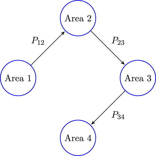
Table 2. An overview of the numerical values used in the simulations, where a base power of 1000 MW is assumed.

		Area 1	Area 2	Area 3	Area 4
$T_{pi}$	(s)	21.0	25.0	23.0	22.0
$T_{ti}$	(s)	0.30	0.33	0.35	0.28
$T_{gi}$	(s)	0.080	0.072	0.070	0.081
$K_{pi}$	(s^−1 p.u.^−1)	120.0	112.5	115.0	118.5
$R_i$	(s^−1 p.u.^−1)	2.5	2.7	2.6	2.8
$T_{\theta i}$	(s)	0.1	0.1	0.1	0.1
$P_{di}\left(0\right)$	(p.u.)	0.010	0.014	0.012	0.013
$P_{di}\left(1\right)$	(p.u.)	0.020	0.028	0.024	0.026

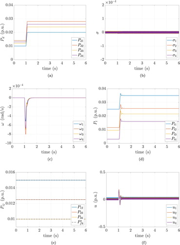
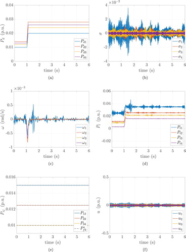
6.1. Scenario 1: step variation of the power demand

At the time instant t=1 s, the power demand in each area becomes $P_{di}\left(1\right)$ (see Table 2 and Figure 3(a)). From Figure 3(b), one can observe that the sliding variables are kept to the manifold $\sigma =\mathbf{0}$. Furthermore, the frequency deviations converge asymptotically to zero after a transient during which the frequency drops because of the increasing load (see Figure 3(c)). From Figure 3(d) one can note that the proposed controllers increase the power generation in order to reach again a zero steady-state frequency deviation, while maintaining, at the steady state, the scheduled power flows $P_{fk}^{\ast }$ on each line (see Figure 3(e)). In Figure 3(f), the control inputs are shown.

Figure 3. (Scenario 1). Power demands, sliding variables, frequency deviations, turbine output powers, power flows on every line and control inputs. The proposed controllers are used with X satisfying (49(49) $X=\epsilon K_p{T}_p^{-1},$(49) ). (a) Power demands, (b) sliding variables, (c) frequency deviations, (d) turbine output powers, (e) power flows and (f) control inputs.

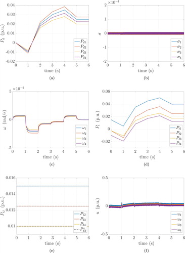
6.2. Scenario 2: time-varying power demand

In this scenario, the power demand continuously changes during the simulation time interval as shown in Figure 4(a). From Figure 4(b), one can observe that the sliding variables are kept to the manifold $\sigma =\mathbf{0}$. Since the power demand is an unknown unmatched external disturbance, the frequency deviations evolve until the power demand becomes constant (see Figure 4(c)). From Figure 4(d), one can note that the proposed controllers continuously adjust the power generation in order to reach again a zero steady-state frequency deviation when the power demand becomes constant. The scheduled power flows $P_{fk}^{\ast }$ on each line are maintained even during the transient (see Figure 4(e)). In Figure 4(f), the control inputs are shown.

Figure 4. (Scenario 2). Power demands, sliding variables, frequency deviations, turbine output powers, power flows on every line and control inputs. The proposed controllers are used with X satisfying (49(49) $X=\epsilon K_p{T}_p^{-1},$(49) ). (a) Power demands, (b) sliding variables, (c) frequency deviations, (d) turbine output powers, (e) power flows and (f) control inputs.

6.3. Scenario 3: measurement noises

Here, we repeat Scenario 1 adding noises in the frequency measuremnets. At the time instant $t=1$ s, the power demand in each area becomes $P_{di}\left(1\right)$ (see Table 2 and Figure 5(a)). From Figure 5(b), one can observe that the sliding variables converge to a vicinity of the origin. Also the frequency deviations converge asymptotically to a vicinity of the origin after a transient during which the frequency drops because of the increasing load (see Figure 5(c)). From Figure 5(d) one can note that the proposed controllers increase the power generation, while maintaining, the scheduled power flows $P_{fk}^{\ast }$ on each line (see Figure 5(e)). In Figure 5(f) the control inputs are shown.

Figure 5. (Scenario 3). Power demands, sliding variables, frequency deviations, turbine output powers, power flows on every line and control inputs, considering noises in the frequency measurements. The proposed controllers are used with X satisfying (49(49) $X=\epsilon K_p{T}_p^{-1},$(49) ). (a) Power demands, (b) sliding variables, (c) frequency deviations, (d) turbine output powers, (e) power flows and (f) control inputs.

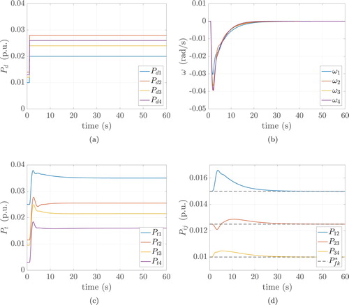
6.4. Scenario 4: comparison with Kundur et al. (1994)

In this subsection, the proposed controller is compared with the conventional automatic generation control law proposed in Kundur et al. (1994), which is given by (51) $u_i\left(t\right)=-K_{Ii}{\int }_0^t{\mathrm{ACE}}_i\left(\tau \right)\mathrm{d}\tau ,$(51) where ACE${}_i$ is known as area control error and is given by (52) ${\mathrm{ACE}}_i\left(t\right)={(\mathcal{B}\mathrm{\Gamma }\sin (\eta )-\mathcal{B}{P}_f^{\ast })}_i+b_i{\omega }_i,$(52) $b_i=1/R_i+1/K_{pi}$ being a suitable bias factor for all areas $i\in \mathcal{V}$ (see Kundur et al., 1994 for more details). We select $K_{Ii}=-0.2$ and repeat Scenario 1, i.e. at the time instant t=1 s, the power demand in each area becomes $P_{di}\left(1\right)$ (see Table 2 and Figure 6(a)). The resulting frequency deviations, turbine output powers and line power flows are provided in Figure 6(b–d), respectively. In comparison with the proposed control scheme in this work (see Figure 3(c–e)), one can notice that the overall response when controller (51(51) $u_i\left(t\right)=-K_{Ii}{\int }_0^t{\mathrm{ACE}}_i\left(\tau \right)\mathrm{d}\tau ,$(51) ) is used, is much slower (note that in the considered scenario the simulation horizon is ten times longer than all the previous scenarios), with larger frequency drops and power flow deviations from the corresponding scheduled values.

Figure 6. (Scenario 4). Power demands, frequency deviations, turbine output powers and power flows on every line. The control law (51(51) $u_i\left(t\right)=-K_{Ii}{\int }_0^t{\mathrm{ACE}}_i\left(\tau \right)\mathrm{d}\tau ,$(51) ) proposed in Kundur et al. (1994) is used. (a) Power demands, (b) frequency deviations, (c) turbine output powers and (d) power flows.

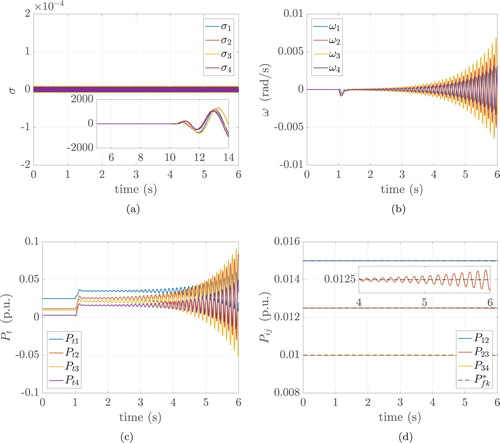
6.5. Scenario 5: condition (49) is not satisfied

To show the importance of the chosen value for ε, we replicate Scenario 1 with $\epsilon =19.5$. One can confirm that this value of ε does not satisfy (49(49) $X=\epsilon K_p{T}_p^{-1},$(49) ). In Figure 7, it is shown that the system, due to the increased value of ε, becomes unstable. Particularly, one can notice that after the system being initially at steady state, the change in power demand causes oscillation of the various states with growing amplitude. Although the system is kept on the sliding manifold for a limited amount of time, the growing amplitude of the various oscillations eventually causes that the sliding condition cannot longer be maintained (see Figure 7 (a)).

Figure 7. (Scenario 5). Sliding variables, frequency deviations, turbine output powers and power flows on every line. The proposed controllers are used with X not satisfying Assumption 5.1. (a) Sliding variables, (b) frequency deviations, (c) turbine output powers and (d) power flows.

7. Conclusions

A decentralised SSOSM control scheme is proposed for LFC. We considered a power network partioned into control areas, where each area is modelled by an equivalent generator including second-order turbine-governor dynamics, and where the areas are nonlinearly coupled through the power flows. Relying on stability considerations made on the basis of an incremental energy (storage) function, a suitable nonlinear sliding function is designed. Local asymptotic convergence is proven to the state where the frequency deviation is zero and where the (net) power flows are identical to their desired values.

Disclosure statement

No potential conflict of interest was reported by the authors.

ORCID

Sebastian Trip  http://orcid.org/0000-0002-6766-6857

Additional information

Funding

This work is supported by the EU Project ‘MatchIT’ (project number: 82203).

Notes

* Preliminary results appeared in Trip, Cucuzzella, Ferrara, and De Persis (2017).

1. For the sake of simplicity, the order r of the sliding manifold is omitted in the remainder of this paper.

2. In case the ‘internal’ governor state $P_{gi}$ or the frequency deviation ω cannot be measured directly, one can rely, e.g. on the sliding mode observers proposed in Rinaldi, Cucuzzella, and Ferrara (2017, 2018) to estimate their values in finite time.

3. The relative degree is the minimum order r of the time derivative ${\sigma }_i^{\left(r\right)},i\in \{1,\dots ,n\}$, of the sliding variable associated to the ith node in which the control $u_i,i\in \{1,\dots ,n\}$, explicitly appears.

4. The peak detector proposed in Bartolini et al. (1998b) requires only the measurement of the sliding function σ, which converges to a ${\rho }^2$-vicinity of the origin, where $\rho >0$ is an arbitrarily small positive constant.

5. Let $[\cos (\eta \left)\right]$ denote the $m\times m$ diagonal matrix $\mathrm{diag}\{\cos ({\eta }_1),\dots ,\cos ({\eta }_m\left)\right\}$.

6. The power network is modelled in MATLAB-Simulink R2018a by using the forward Euler method with sampling time interval ${\tau }_s=1\times {10}^{-3}\mathrm{s}$. Then, according to Shtessel et al. (2014), the corresponding discrete-sampling version provides an accuracy level of $\sigma =O\left({\tau }_s^2\right),\dot{\sigma }=O\left({\tau }_s\right)$.

References

- Apostolopoulou, D., Domínguez-García, A. D., & Sauer, P. W. (2016, July). An assessment of the impact of uncertainty on automatic generation control systems. IEEE Transactions on Power Systems, 31(4), 2657–2665.
- Bapat, R. B. (2010). Graphs and matrices. Springer.
- Bartolini, G., Ferrara, A., & Usai, E. (1998a, February). Chattering avoidance by second-order sliding mode control. IEEE Transactions on Automatic Control, 43(2), 241–246.
- Bartolini, G., Ferrara, A., & Usai, E. (1998b, September). On boundary layer dimension reduction in sliding mode control of SISO uncertain nonlinear systems. Proceedings of the IEEE internation conference on control applications (pp. 242–247). Trieste, Italy.
- Bregman, L. (1967). The relaxation method of finding the common point of convex sets and its application to the solution of problems in convex programming. USSR Computational Mathematics and Mathematical Physics, 7(3), 200–217.
- Chang, C., & Fu, W. (1997, August). Area load frequency control using fuzzy gain scheduling of PI controllers. Electric Power Systems Research, 42(2), 145–152.
- Dong, L. (2016, July). Decentralized load frequency control for an interconnected power system with nonlinearities. Proceedings of the IEEE American control conference (pp. 5915–5920). Boston, MA.
- Dvijotham, K., Low, S., & Chertkov, M. (2015). Convexity of energy-like functions: Theoretical results and applications to power system operations. arXiv preprint arXiv:1501.04052v3.
- Edwards, C., & Spurgen, S. K. (1998). Sliding mode control: Theory and applications. London: Taylor and Francis.
- Ersdal, A. M., Imsland, L., & Uhlen, K. (2016, January). Model predictive load-frequency control. IEEE Transactions on Power Systems, 31(1), 777–785.
- Furtat, I. B., & Fradkov, A. L. (2015, December). Robust control of multi-machine power systems with compensation of disturbances. International Journal of Electrical Power & Energy Systems, 73, 584–590.
- Ha, Q. P. (1998, April). A fuzzy sliding mode controller for power system load-frequency control. Knowledge-based intelligent electronic systems (pp. 149–154). Adelaide, SA.
- Ibraheem, N., Kumar, P., & Kothari, D. P. (2005, February). Recent philosophies of automatic generation control strategies in power systems. IEEE transactions on Power Systems, 20(1), 346–357.
- Incremona, G. P., Cucuzzella, M., & Ferrara, A. (2016, January). Adaptive suboptimal second-order sliding mode control for microgrids. International Journal of Control, 89(9), 1849–1867.
- Kundur, P., Balu, N. J., & Lauby, M. G. (1994). Power system stability and control. New York, NY: McGraw-hill.
- Levant, A. (1993). Sliding order and sliding accuracy in sliding mode control. International Journal of Control, 58(6), 1247–1263.
- Levant, A. (2003, January). Higher-order sliding modes, differentiation and output-feedback control. International Journal of Control, 76(9–10), 924–941.
- Mi, Y., Fu, Y., Li, D., Wang, C., Loh, P. C., & Wang, P. (2016, January). The sliding mode load frequency control for hybrid power system based on disturbance observer. International Jorunal of Electrical Power and Energy Systems, 74, 446–452.
- Mi, Y., Fu, Y., Wang, C., & Wang, P. (2013, November). Decentralized sliding mode load frequency control for multi-area power systems. IEEE Transactions on Power Systems, 28(4), 4301–4309.
- Pandey, S. K., Mohanty, S. R., & Kishor, N. (2013, September). A literature survey on load–frequency control for conventional and distribution generation power systems. Renewable and Sustainable Energy Reviews, 25, 318–334.
- Pogromsky, A. Y., Fradkov, A. L., & Hill, D. J. (1996, December). Passivity based damping of power system oscillations. Proceedings of 35th IEEE conference on decision and control (pp. 3876–3881). Kobe.
- Prasad, S., Purwar, S., & Kishor, N. (2015, September). On design of a non-linear sliding mode load frequency control of interconnected power system with communication time delay. Proceedings of the IEEE conference on control applications (pp. 1546–1551). Sydney.
- Rinaldi, G., Cucuzzella, M., & Ferrara, A. (2017, October). Third order sliding mode observer-based approach for distributed optimal load frequency control. IEEE Control Systems Letters, 1(2), 215–220.
- Rinaldi, G., Cucuzzella, M., & Ferrara, A. (2018). Sliding mode observers for a network of thermal and hydroelectric power plants. Automatica, 98, 51–57.
- Shtessel, Y., Edwards, C., Fridman, L., & Levant, A. (2014). Conventional sliding mode observers. In Sliding mode control and observation (pp. 105–141). Springer.
- Trip, S., Bürger, M., & De Persis, C. (2016). An internal model approach to (optimal) frequency regulation in power grids with time-varying voltages. Automatica, 64, 240–253.
- Trip, S., Cucuzzella, M., Ferrara, A., & De Persis, C. (2017, July). An energy function based design of second order sliding modes for automatic generation control. IFAC-PapersOnLine, 50(1), 11613–11618. (20th IFAC World Congres)
- Trip, S., Cucuzzella, M., Persis, C. D., van der Schaft, A., & Ferrara, A. (2018). Passivity-based design of sliding modes for optimal load frequency control. IEEE Transactions on Control Systems Technology.
- Trip, S., & De Persis, C. (2018, September). Distributed optimal load frequency control with non-passive dynamics. IEEE Transactions on Control of Network Systems, 5(3), 1232–1244.
- Utkin, V. (2016, March). Discussion aspects of high-order sliding mode control. IEEE Transactions on Automatic Control, 61(3), 829–833.
- Utkin, V. I. (1992). Sliding modes in control and optimization. Springer-Verlag.
- Ventura, U. P., & Fridman, L. (2016, June). Chattering measurement in SMC and HOSMC. 2016 14th international workshop on variable structure systems (VSS) (pp. 108–113). Nanjing.
- Vrdoljak, K., Perić, N., & Petrović, I. (2010, May). Sliding mode based load-frequency control in power systems. Electrocal Power Systems Research, 80(5), 514–527.
- Vu, T. L., & Turitsyn, K. (2016, March). Lyapunov functions family approach to transient stability assessment. IEEE Transactions on Power Systems, 31(2), 1269–1277.
- Zribi, M., Al-Rashed, M., & Alrifai, M. (2005, October). Adaptive decentralized load frequency control of multi-area power systems. International Jorunal on Electrical Power and Energy Systems, 27(8), 575–583.