Event-triggered variable structure control

ABSTRACT

This paper presents a novel variable structure control (VSC) algorithm of event-triggered (ET) type, capable of dealing with a class of nonlinear uncertain systems. By virtue of its ET nature, the algorithm can be used as the kernel of a robust networked control system. The design objective is indeed to reduce the number of transmissions over the network. The proposed ET-VSC also guarantees appropriate robustness properties, even in the presence of delayed transmissions. It is theoretically analysed, proving that the sliding variable associated with the controlled system results in being ultimately confined into a boundary layer of prescribed amplitude. As a consequence, it is proved that the state of the considered uncertain nonlinear system is ultimately bounded as well. Moreover, a lower bound for the time elapsed between consecutive triggering events is provided, which excludes the notorious Zeno behaviour. Finally, the designed ET-VSC control scheme is satisfactorily assessed in simulation.

KEYWORDS:

• Variable structure control
• sliding mode control
• uncertain systems

1. Introduction

Sliding mode control (SMC) is an effective methodology able to guarantee satisfactory performance of the controlled system even in the presence of matched uncertainties and external disturbances (Utkin, 1992, 1994). By virtue of its low implementation complexity, it can be adequate also in case of networked control systems (NCSs), i.e. feedback systems including communication networks (Hespanha, Naghshtabrizi, & Xu, 2007).

In those systems, the presence of the network in the control loop may cause the occurrence of packet loss, jitter, and delayed transmissions, which can deteriorate the performance of the control system (Wang & Liu, 2008). Since the network malfunctions tend to increase with the network congestion, the design of control approaches aimed at reducing the transmissions over the network is often resolutive.

A methodology which is very appreciated to design NCSs is the so-called event-triggered (ET) control (Aström, 2008; De Persis, Sailer, & Wirth, 2013; De Persis & Tesi, 2015; Heemels, Sandee, & Van Den Bosch, 2008; Tabuada, 2007; You & Xie, 2013; Yu & Antsaklis, 2011). ET control, in contrast to time-triggered control, which features periodic transmissions of the measurements, enables the measurement transmissions only when a pre-specified triggering condition is satisfied (or violated, depending on the adopted logic). This implies that the number of transmissions over the network can be significantly reduced by suitably setting the triggering condition threshold. By using ET control, in spite of the aperiodic transmission of the measurements, satisfactory stability properties can be enforced. Note that the basic ET control approach has been further elaborated so as to take into account the possible knowledge of a nominal model of the plant. This has produced the model-based event-triggered control discussed in Garcia and Antsaklis (2011) and Montestruque and Antsaklis (2004).

ET control has been recently effectively exploited in conjunction with SMC and model predictive control (MPC) (see Cucuzzella & Ferrara, 2016, 2018; Ferrara & Cucuzzella, 2018; Ferrara, Sacone, & Siri, 2015a, 2015b; Incremona & Ferrara, 2016; Incremona, Ferrara, & Magni, 2017). It is worth noticing however that when SMC is coupled with the ET approach, the attainment of an ideal sliding mode (SM) is not feasible (Behera & Bandyopadhyay, 2016; Behera, Bandyopadhyay, Xavier, & Kamal, 2015), this is why we prefer to use in this paper the term ‘ Variable Structure Control’ (VSC) to classify the proposed approach.

Specifically, in this paper, we propose a novel VSC algorithm of event-triggered type, capable of dealing with a class of nonlinear uncertain systems. The control problem to solve is challenging because the considered system is a nonlinear system affected by uncertain terms which are exogenous signals, functions of time, and the considered control architecture is of networked type (i.e. a communication network is used to implement the control scheme), which implies that time delays can affect the control variable/state transmission. In addition, we want to comply with the requirement of utilising the communication network, which can be considered as a critical resource, with parsimony.

The proposed algorithm is theoretically analysed in the paper, proving that the sliding variable associated with the controlled system results in being ultimately confined into a boundary layer of prescribed amplitude. As a consequence, it is proved that the state of the considered uncertain nonlinear system is ultimately bounded as well. It is worth noting that the obtained evolution of the sliding variable within a boundary layer implies that the state of the controlled system eventually reaches and remains inside a ball centred at the equilibrium point of interest, this ball in fact being an ultimately positively invariant set of the controlled system. Note that this behaviour can resemble that of the classical switching control with hysteresis (see Utkin, 1992), with the difference that in the proposed control strategy the system state and the control input are not always transmitted. As a further result, a lower bound for the time elapsed between consecutive triggering events is provided in the paper, which excludes the existence of an accumulation point, i.e. the notorious Zeno phenomenon, also known as ‘Fuller phenomenon’ (see Liberzon, 2003) and long recognised in sliding mode theory (Ames, Tabuada, & Sastry, 2006; Johansson, Lygeros, Sastry, & Egerstedt, 1999; Yu et al., 2012). All the paper results have been proved in spite of the possible presence of transmission delays.

Note that our contribution differs from those already published in the literature and previously mentioned. In Behera and Bandyopadhyay (2017), for instance, ET is combined with SMC in order to guarantee the robust global stability of linear time-invariant systems affected by matched external disturbances. Differently from the present work, the triggering condition proposed in Behera and Bandyopadhyay (2017) is based on the error between the actual state and the one previously transmitted, while the threshold is not constant and depends on the sampled state. A model-based ET is used in connection with SMC in Incremona and Ferrara (2016), while second-order SMC laws are considered in Cucuzzella and Ferrara (2018). Note however that both the last two papers do not consider the presence of transmission delays.

Note that a very preliminary version of the theory presented in this paper, where no communication delay was considered, and the proofs of the theoretical results, as well as the discussion about the Zeno behaviour were not included, was provided in Cucuzzella, Incremona, and Ferrara (2016).

Finally, we wish to underline that the authors present this work to celebrate the 70th anniversary of Professor Fradkov. In particular, we have selected the specific paper topics inspired by the vast literature by Professor Fradkov on nonlinear dynamics and hybrid systems (see, for instance, Fradkov, Miroshnik, & Nikiforov, 1999; Leonov, Nijmeijer, Pogromsky, & Fradkov, 2010). Indeed, the event-triggered variable structure control proposed in this paper gives rise to a controlled system which can be classified as a particular case of hybrid system (van der Schaft & Schumacher, 2000).

The present paper is organised as follows. In Section 2, the control problem under consideration is suitably formulated. The proposed control strategy is described in Section 3. In Section 4, the stability properties of the overall ET-VSC scheme are formally discussed. The simulation results are illustrated in Section 5 to demonstrate the efficacy of the proposal. Some conclusions are finally gathered in Section 6.

2. Problem formulation

In the following sections, $\parallel \cdot \parallel$ will denote the Euclidean norm for vectors and the induced Euclidean norm for matrices, $\mid \cdot \mid$ will denote the absolute value, and $⟨a,b⟩$ will denote the scalar product between vectors a and b. Given the set $\mathcal{W}\subset \mathbb{R}$, $w^{sup}\triangleq \underset{\begin{array}{c}w\in \mathcal{W}\end{array}}{sup}\left\{\mid w\mid \right\}$. The relative degree of the system, i.e. the minimum order r of the time derivative ${\sigma }^{\left(r\right)}$ of the output function in which the control u explicitly appears, is considered well defined, uniform and time-invariant.

Consider a plant (process and actuator) which can be modelled as (1) $\begin{array}{rl}{\dot{x}}_i\left(t\right)& =x_{i+1}\left(t\right),i=1,\dots ,n-1,\\ {\dot{x}}_n\left(t\right)& =f\left(x\right(t),t)+b\left(x\right(t),t)\left(u\right(t)+w(t\left)\right),\end{array}$(1) where $x\in \mathrm{\Omega }$ ($\mathrm{\Omega }\subset {\mathbb{R}}^n$ bounded) is the state vector the value of which at the initial time instant $t_0$ is $x\left(t_0\right)=x_0$, $u\in \mathbb{R}$ is the control variable, $f:\mathrm{\Omega }\times \mathbb{R}\to \mathbb{R}$, $b:\mathrm{\Omega }\times \mathbb{R}\to \mathbb{R}$ are bounded uncertain functions, and $w:\mathbb{R}\to \mathbb{R}$ is a bounded external disturbance such that the following assumptions on the uncertainty terms hold .¹

Assumption 2.1

Boundedness of the functions f and b

There exist known positive constants F, $B_{min}$ and $B_{max}$ such that for any $x\in \mathrm{\Omega }$ and $t\ge t_0$, the functions f and b in system (1(1) $\begin{array}{rl}{\dot{x}}_i\left(t\right)& =x_{i+1}\left(t\right),i=1,\dots ,n-1,\\ {\dot{x}}_n\left(t\right)& =f\left(x\right(t),t)+b\left(x\right(t),t)\left(u\right(t)+w(t\left)\right),\end{array}$(1) ) satisfy (2) $\begin{array}{rl}& \mid f\left(x\right(t),t)\mid \le F,\end{array}$(2) (3) $\begin{array}{rl}& 0<B_{min}\le b\left(x\right(t),t)\le B_{max}.\end{array}$(3)

Assumption 2.2

Boundedness of the disturbance w

For any $t\ge t_0$, the external disturbance w in system (1(1) $\begin{array}{rl}{\dot{x}}_i\left(t\right)& =x_{i+1}\left(t\right),i=1,\dots ,n-1,\\ {\dot{x}}_n\left(t\right)& =f\left(x\right(t),t)+b\left(x\right(t),t)\left(u\right(t)+w(t\left)\right),\end{array}$(1) ) satisfies (4) $w\in \mathcal{W},$(4) $w^{sup}$ being a known positive constant.

Let $\sigma :\mathrm{\Omega }\to \mathcal{Y}\subseteq \mathbb{R}$ be the output function of system (1(1) $\begin{array}{rl}{\dot{x}}_i\left(t\right)& =x_{i+1}\left(t\right),i=1,\dots ,n-1,\\ {\dot{x}}_n\left(t\right)& =f\left(x\right(t),t)+b\left(x\right(t),t)\left(u\right(t)+w(t\left)\right),\end{array}$(1) ). Then, the problem to solve is to design a control law u able to stabilise system (1(1) $\begin{array}{rl}{\dot{x}}_i\left(t\right)& =x_{i+1}\left(t\right),i=1,\dots ,n-1,\\ {\dot{x}}_n\left(t\right)& =f\left(x\right(t),t)+b\left(x\right(t),t)\left(u\right(t)+w(t\left)\right),\end{array}$(1) ) even in the presence of uncertainties and delayed transmissions due to the communication networks represented in Figure 1. More specifically, we require that σ is ultimately bounded in a prescribed vicinity of the manifold $\sigma =0$.

Figure 1. The proposed event-triggered variable structure control scheme.

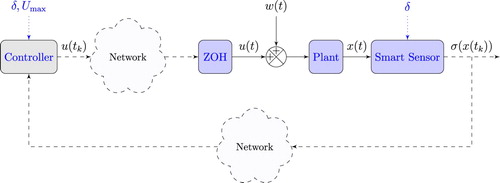
3. The proposal: event-triggered variable structure control for NCSs

In practical implementation the state is sampled at certain time instants $t\in \{t_0,t_1,\dots t_k,\dots \},k\in \mathbb{N}$, and the input, computed as $u\left(t_k\right)=\kappa \left(\sigma \right(x\left(t_k\right)\left)\right)$, with κ being a generic control law depending on $\sigma \left(x\right(t_k\left)\right)$ to be designed, is held constant between two successive samplings. This kind of implementation, called sample-and-hold, can be expressed as (5) $u\left(t\right)=u\left(t_k\right),\mathrm{\forall }t\in [t_k,t_{k+1}[,k\in \mathbb{N},$(5) where $t_k,t_{k+1}\in \mathcal{T}$, $\mathcal{T}$ being the set of the triggering time instants. In conventional implementation, the sequence $\{t_k{\}}_{k\in \mathbb{N}}$ is typically periodic and the time interval $t_{k+1}-t_k$, is a priori fixed. The control approach, in that case, is classified as time-triggered.

In the present paper, instead of relying on time-triggered executions, we introduce a triggering condition which depends on σ, so that the state of the controlled plant is transmitted over the network only when such a condition is verified. This implies that the control law is updated and sent to the plant only at the triggering time instants, and the overall control strategy is of event-triggered type. Note that, in this paper, we do not adopt a mathematical model of the network, but we design the control strategy in such a way to reduce data transmission as much as possible. This in order to limit the negative effects of the network congestion, such as packets drop, jitter, and delays. However, we suppose that the presence of the communication network can cause delayed transmissions due to the network unavailability or packet losses. Moreover, we assume that the plant is equipped with a zero-order-hold (ZOH) so that the control variable computed at the last triggering time instant $t_k$ is held constant $\mathrm{\forall }t\in [t_k,t_{k+1}[$. Then, this approach tends to reduce the transmissions over the network both in the direct path (from the controller to the plant) and in the feedback path (from the sensor to the controller). Now, consider the control scheme reported in Figure 1. It contains two key blocks: the smart sensor and the sliding mode controller. These blocks are hereafter detailed.

3.1. The smart sensor

We assume that the considered sensor is smart in the sense that it has some computation capability, i.e. it is able to compute (in the continuous time) the controlled variable σ and verify a triggering condition. The triggering condition adopted in this paper is the following: (6) $\mid \sigma \left(x\right(t\left)\right)\mid =\delta ,$(6) δ being a positive constant arbitrarily set. Only when the triggering condition (6(6) $\mid \sigma \left(x\right(t\left)\right)\mid =\delta ,$(6) ) holds (i.e. at the triggering time instant $t=t_k$, $t_k\in \mathcal{T}$) is the actual output $\sigma \left(t_k\right)$ transmitted by the sensor over the network, so that the control law is updated and $u\left(t_k\right)$ sent to the plant.

3.2. The controller

To solve the problem formulated in Section 2, in this paper, we rely on the SMC methodology (Utkin, 1992), and design an event-triggered variable structure control (ET-VSC) scheme. To this end, we denote the output function σ as the so-called ‘sliding variable’, with $\sigma =0$ being the so-called ‘sliding manifold’ and design it as a linear combination of the system state, i.e. (7) $\sigma \left(x\right(t\left)\right)=\sum _{i=1}^{n-1}{m}_i{x}_i\left(t\right)+x_n\left(t\right),$(7) with $m_i,i=1,\dots ,n-1$, real positive constants such that the characteristic equation $\sum _{i=1}^{n-1}{m}_i{z}^{i-1}+z^{n-1}=0$ has distinct roots with negative real part. By regarding (7(7) $\sigma \left(x\right(t\left)\right)=\sum _{i=1}^{n-1}{m}_i{x}_i\left(t\right)+x_n\left(t\right),$(7) ) as the controlled variable, associated with system (1(1) $\begin{array}{rl}{\dot{x}}_i\left(t\right)& =x_{i+1}\left(t\right),i=1,\dots ,n-1,\\ {\dot{x}}_n\left(t\right)& =f\left(x\right(t),t)+b\left(x\right(t),t)\left(u\right(t)+w(t\left)\right),\end{array}$(1) ), it turns out that the relative degree r of the input–output map is 1, so that the so-called ‘auxiliary system’ can be determined as follows: (8) $\begin{array}{rl}\dot{\sigma }\left(x\right(t\left)\right)& =\sum _{i=1}^{n-1}{m}_i{x}_{i+1}\left(t\right)+f\left(x\right(t),t)+b\left(x\right(t),t)\left(u\right(t)+w(t\left)\right)\\ & =\varphi \left(x\right(t),t)+b\left(x\right(t),t)u\left(t\right),\end{array}$(8) where $\varphi =\sum _{i=1}^{n-1}{m}_i{x}_{i+1}+f+bw$, such that the following assumption holds.

Assumption 3.1

Boundedness of the function ϕ

For any $x\in \mathrm{\Omega }$ and $t\ge t_0$, the uncertain function $\varphi \left(x\right(t),t)$ in (8(8) $\begin{array}{rl}\dot{\sigma }\left(x\right(t\left)\right)& =\sum _{i=1}^{n-1}{m}_i{x}_{i+1}\left(t\right)+f\left(x\right(t),t)+b\left(x\right(t),t)\left(u\right(t)+w(t\left)\right)\\ & =\varphi \left(x\right(t),t)+b\left(x\right(t),t)u\left(t\right),\end{array}$(8) ) satisfies (9) $\mid \varphi \left(x\right(t),t)\mid \le {\mathrm{\Phi }}^{sup},$(9) ${\mathrm{\Phi }}^{sup}$ being a positive constant.

Remark 3.1

Local boundedness

If Ω is equal to ${\mathbb{R}}^n$, then $\varphi \left(x\right(t),t)$ is only locally bounded. In this case, characterising the region of attraction requires a careful analysis of the considered system. Although in practical cases the region of attraction can be estimated relaying on e.g. data analysis or physical insights, a thorough analysis of the region of attraction is outside the scope of this paper.

The proposed control law at the triggering time instants, namely $u\left(t_k\right)$, $k\in \mathbb{N}$, can be expressed as (10) $u\left(t_k\right)=-U_{max}\mathrm{s}\mathrm{i}\mathrm{g}\mathrm{n}\left(\sigma \right(x\left(t_k\right)\left)\right),$(10) with (11) $U_{max}>\frac{{\mathrm{\Phi }}^{sup}}{B_{min}}.$(11) The sample-and-hold mechanism (5(5) $u\left(t\right)=u\left(t_k\right),\mathrm{\forall }t\in [t_k,t_{k+1}[,k\in \mathbb{N},$(5) ), with control law $u\left(t_k\right)$ as in (10(10) $u\left(t_k\right)=-U_{max}\mathrm{s}\mathrm{i}\mathrm{g}\mathrm{n}\left(\sigma \right(x\left(t_k\right)\left)\right),$(10) ), and the triggering condition (6(6) $\mid \sigma \left(x\right(t\left)\right)\mid =\delta ,$(6) ) give rise to the ET-VSC strategy that we propose to steer the sliding variable σ in a finite time $t_{\mathrm{r},\sigma }\ge t_0$ to the prescribed boundary layer ${\mathcal{B}}_{\delta }\subseteq \sigma \left(\mathrm{\Omega }\right)$, defined as a vicinity of the sliding manifold $\sigma =0$, i.e. (12) ${\mathcal{B}}_{\delta }\triangleq \left\{\sigma \in \sigma \left(\mathrm{\Omega }\right):\mid \sigma \mid \le \delta \right\},$(12) δ being a positive constant arbitrarily set. Moreover, let ${\mathrm{\Omega }}_{\delta }\triangleq \{x\in \mathrm{\Omega }:\mid \sigma \left(x\right)\mid \le \delta \}$, ${\mathrm{\Omega }}_{\delta }\subseteq \mathrm{\Omega }$. Then, inside the boundary layer ${\mathcal{B}}_{\delta }$, the following assumption holds.

Assumption 3.2

Boundedness of the functions f, b and ϕ when $\sigma \in {\mathcal{B}}_{\delta }$

For any $x\in {\mathrm{\Omega }}_{\delta }$ and $t\ge t_{\mathrm{r},\sigma }$, i.e. when $\sigma \in {\mathcal{B}}_{\delta }$, the uncertain functions f, b and ϕ satisfy (13) $\begin{array}{rl}& \mid f\left(x\right(t),t)\mid \le F_{\delta },\end{array}$(13) (14) $\begin{array}{rl}& 0<B_{\delta ,min}\le b\left(x\right(t),t)\le B_{\delta ,max},\end{array}$(14) (15) $\begin{array}{rl}& \mid \varphi \left(x\right(t),t)\mid \le {\mathrm{\Phi }}_{\delta }^{sup},\end{array}$(15) where $F_{\delta }\le F,B_{\delta ,min}\ge B_{min},B_{\delta ,max}\le B_{max}$, and ${\mathrm{\Phi }}_{\delta }^{sup}\le {\mathrm{\Phi }}^{sup}$ are known positive constants.

Remark 3.2

Control effort reduction

By virtue of the inequalities (13(13) $\begin{array}{rl}& \mid f\left(x\right(t),t)\mid \le F_{\delta },\end{array}$(13) )–(15(15) $\begin{array}{rl}& \mid \varphi \left(x\right(t),t)\mid \le {\mathrm{\Phi }}_{\delta }^{sup},\end{array}$(15) ), in order to reduce the control effort and the number of triggering events when the sliding variable σ enters the boundary layer ${\mathcal{B}}_{\delta }$, the amplitude of the control law can be reduced, i.e. (16) $u\left(t_k\right)=-K{U}_{max}\mathrm{s}\mathrm{i}\mathrm{g}\mathrm{n}\left(\sigma \right(x\left(t_k\right)\left)\right),$(16) with (17) $\frac{{\mathrm{\Phi }}_{\delta }^{sup}}{B_{\delta ,min}{U}_{max}}<K<1$(17) and $U_{max}$ as in (11(11) $U_{max}>\frac{{\mathrm{\Phi }}^{sup}}{B_{min}}.$(11) ).

Remark 3.3

Potentiality of ET-VSC

Note that the proposed ET-VSC approach could be extended to the so-called vector relay control, also referred as unit-vector control (Edwards & Spurgen, 1998; Orlov & Utkin, 1998). In fact, event-triggered strategies may be attractive for various applications in which vector relay control is typically applied. Specifically, vector relay control can be used for drive control application or for regulating voltage converters, where, although a hysteretic approach is often used, time-varying parameters, communication networks as well as unpredictable noise spectrum make the electromagnetic interference control problem particularly difficult to solve (see for instance Ryvkin & Palomar Lever, 2011; Tan, Lai, & Tse, 2017).

4. Stability analysis

In this section, the stability properties of system (1(1) $\begin{array}{rl}{\dot{x}}_i\left(t\right)& =x_{i+1}\left(t\right),i=1,\dots ,n-1,\\ {\dot{x}}_n\left(t\right)& =f\left(x\right(t),t)+b\left(x\right(t),t)\left(u\right(t)+w(t\left)\right),\end{array}$(1) ) controlled via the proposed ET-VSC strategy are analysed. To this end, it is convenient to introduce the following definitions:

Definition 4.1

Reachability condition

The set ${\mathcal{B}}_{\delta }$ is said to be attractive if the solution to the uncertain system (8(8) $\begin{array}{rl}\dot{\sigma }\left(x\right(t\left)\right)& =\sum _{i=1}^{n-1}{m}_i{x}_{i+1}\left(t\right)+f\left(x\right(t),t)+b\left(x\right(t),t)\left(u\right(t)+w(t\left)\right)\\ & =\varphi \left(x\right(t),t)+b\left(x\right(t),t)u\left(t\right),\end{array}$(8) ), $\mathrm{\forall }\sigma \in \mathbb{R}\setminus {\mathcal{B}}_{\delta }$, satisfies the so-called η-reachability condition (see Utkin, 1992) (18) $\sigma \dot{\sigma }\le -\eta \mid \sigma \mid .$(18)

Definition 4.2

Ultimately boundedness

The solution σ to the uncertain system (8(8) $\begin{array}{rl}\dot{\sigma }\left(x\right(t\left)\right)& =\sum _{i=1}^{n-1}{m}_i{x}_{i+1}\left(t\right)+f\left(x\right(t),t)+b\left(x\right(t),t)\left(u\right(t)+w(t\left)\right)\\ & =\varphi \left(x\right(t),t)+b\left(x\right(t),t)u\left(t\right),\end{array}$(8) ) is said to be ultimately bounded with respect to the set ${\mathcal{B}}_{\delta }$ if in a finite time $t_{\mathrm{r},\sigma }$ it enters the bounded set ${\mathcal{B}}_{\delta }$ and remains there for all subsequent time instants.

Definition 4.3

Positively invariant set

Let σ be the solution to the uncertain system (8(8) $\begin{array}{rl}\dot{\sigma }\left(x\right(t\left)\right)& =\sum _{i=1}^{n-1}{m}_i{x}_{i+1}\left(t\right)+f\left(x\right(t),t)+b\left(x\right(t),t)\left(u\right(t)+w(t\left)\right)\\ & =\varphi \left(x\right(t),t)+b\left(x\right(t),t)u\left(t\right),\end{array}$(8) ) starting from the initial condition $\sigma \left(x_0\right)$. A set ${\mathcal{B}}_{\delta }$ is said to be positively invariant if $\sigma \left(x_0\right)\in {\mathcal{B}}_{\delta }$ implies that $\sigma \left(x\right(t\left)\right)\in {\mathcal{B}}_{\delta },\mathrm{\forall }t\ge t_0$.

Now, making reference to (8(8) $\begin{array}{rl}\dot{\sigma }\left(x\right(t\left)\right)& =\sum _{i=1}^{n-1}{m}_i{x}_{i+1}\left(t\right)+f\left(x\right(t),t)+b\left(x\right(t),t)\left(u\right(t)+w(t\left)\right)\\ & =\varphi \left(x\right(t),t)+b\left(x\right(t),t)u\left(t\right),\end{array}$(8) ) the following results can be proved.

Lemma 4.1

Attractiveness of ${\mathcal{B}}_{\delta }$

Let the sign of the initial condition $\sigma \left(x_0\right)$ be known and let $\mid \sigma \left(x_0\right)\mid >\delta$, with $\delta >0$ arbitrarily set. Given system (8(8) $\begin{array}{rl}\dot{\sigma }\left(x\right(t\left)\right)& =\sum _{i=1}^{n-1}{m}_i{x}_{i+1}\left(t\right)+f\left(x\right(t),t)+b\left(x\right(t),t)\left(u\right(t)+w(t\left)\right)\\ & =\varphi \left(x\right(t),t)+b\left(x\right(t),t)u\left(t\right),\end{array}$(8) ) controlled by (5(5) $u\left(t\right)=u\left(t_k\right),\mathrm{\forall }t\in [t_k,t_{k+1}[,k\in \mathbb{N},$(5) ), (10(10) $u\left(t_k\right)=-U_{max}\mathrm{s}\mathrm{i}\mathrm{g}\mathrm{n}\left(\sigma \right(x\left(t_k\right)\left)\right),$(10) ) with (11(11) $U_{max}>\frac{{\mathrm{\Phi }}^{sup}}{B_{min}}.$(11) ) and the triggering condition (6(6) $\mid \sigma \left(x\right(t\left)\right)\mid =\delta ,$(6) ), then, the boundary layer ${\mathcal{B}}_{\delta }$ is attractive for any solution σ to (8(8) $\begin{array}{rl}\dot{\sigma }\left(x\right(t\left)\right)& =\sum _{i=1}^{n-1}{m}_i{x}_{i+1}\left(t\right)+f\left(x\right(t),t)+b\left(x\right(t),t)\left(u\right(t)+w(t\left)\right)\\ & =\varphi \left(x\right(t),t)+b\left(x\right(t),t)u\left(t\right),\end{array}$(8) ).

Proof.

Consider the η-reachability condition (18(18) $\sigma \dot{\sigma }\le -\eta \mid \sigma \mid .$(18) ). Taking into account that the initial condition $\sigma \left(x_0\right)={\sigma }_0$ is known, one has that $sign\left(\sigma \right(x\left(t\right)\left)\right)=sign\left({\sigma }_0\right),\mathrm{\forall }t\in [t_0,t_1]$, $t_1$ being the first triggering time instant satisfying $\mid \sigma \left(x\right(t_1\left)\right)\mid =\delta$. Making reference to system (8(8) $\begin{array}{rl}\dot{\sigma }\left(x\right(t\left)\right)& =\sum _{i=1}^{n-1}{m}_i{x}_{i+1}\left(t\right)+f\left(x\right(t),t)+b\left(x\right(t),t)\left(u\right(t)+w(t\left)\right)\\ & =\varphi \left(x\right(t),t)+b\left(x\right(t),t)u\left(t\right),\end{array}$(8) ), since $\sigma \mathrm{s}\mathrm{i}\mathrm{g}\mathrm{n}\left(\sigma \right)=\mid \sigma \mid$, during the time interval $[t_0,t_1]$ it yields (19) $\begin{array}{rl}\sigma \left(x\right(t\left)\right)\dot{\sigma }\left(x\right(t\left)\right)& =\sigma \left(x\right(t\left)\right)\left(\sum _{i=1}^{n-1}{m}_i{\dot{x}}_i\left(t\right)+{\dot{x}}_n\left(t\right)\right)\\ & =\sigma \left(x\right(t\left)\right)\left(\sum _{i=1}^{n-1}{m}_i{\dot{x}}_i\left(t\right)+f\left(x\right(t),t)\right.\\ & \left.+b\left(x\right(t),t)\left(u\right(t_0)+w(t\left)\right)\phantom{\sum _{i=1}^{n-1}{m}_i{\dot{x}}_i\left(t\right)+{\dot{x}}_n\left(t\right)}\right)\\ & =\sigma \left(x\right(t\left)\right)\left(\varphi \left(x\right(t),t)+b\left(x\right(t),t)u\left(t_0\right)\right)\\ & =\sigma \left(x\right(t\left)\right)\left(\varphi \left(x\right(t),t)-b\left(x\right(t),t)U_{max}\mathrm{s}\mathrm{i}\mathrm{g}\mathrm{n}\left({\sigma }_0\right)\right)\\ & \le \left({\mathrm{\Phi }}^{sup}-B_{min}{U}_{max}\right)\mid \sigma \left(x\right(t\left)\right)\mid .\end{array}$(19) Since (11(11) $U_{max}>\frac{{\mathrm{\Phi }}^{sup}}{B_{min}}.$(11) ) holds, then, one can verify that ${\mathrm{\Phi }}^{sup}-B_{min}{U}_{max}<0,$ that is (18(18) $\sigma \dot{\sigma }\le -\eta \mid \sigma \mid .$(18) ) holds with $\eta =-({\mathrm{\Phi }}^{sup}-B_{min}{U}_{max})>0$. Then, integrating the inequality $\sigma \dot{\phantom{a}}\sigma \le -\eta \mid \sigma \mid$ from $t_0=0$ to $t_{\mathrm{r},\sigma }$, one has (20) $t_{\mathrm{r},\sigma }\le \frac{\mid \sigma \left(0\right)\mid -\delta }{\eta },$(20) implying the finite time convergence of the sliding variable to ${\mathcal{B}}_{\delta }$. Moreover, one can conclude that the first transmission over the network is executed at the triggering time instant $t_1=t_{\mathrm{r},\sigma }$.

Remark 4.4

Reaching phase

Note that, by virtue of Lemma 4.1, the proposed control solution avoids to transmit the value of σ and u over the networks during the entire reaching phase, i.e. till the sliding variable enters the boundary layer ${\mathcal{B}}_{\delta }$ at the time instant $t_{\mathrm{r},\sigma }$.

Lemma 4.2

Invariance of ${\mathcal{B}}_{\delta }$

Given system (8(8) $\begin{array}{rl}\dot{\sigma }\left(x\right(t\left)\right)& =\sum _{i=1}^{n-1}{m}_i{x}_{i+1}\left(t\right)+f\left(x\right(t),t)+b\left(x\right(t),t)\left(u\right(t)+w(t\left)\right)\\ & =\varphi \left(x\right(t),t)+b\left(x\right(t),t)u\left(t\right),\end{array}$(8) ) with the initial condition $\sigma \left(x_0\right)$ such that $\mid \sigma \left(x_0\right)\mid \le \delta ,$ with $\delta >0$ arbitrarily set, then, the boundary layer ${\mathcal{B}}_{\delta }$ is a positively invariant set for the solution σ to system (8(8) $\begin{array}{rl}\dot{\sigma }\left(x\right(t\left)\right)& =\sum _{i=1}^{n-1}{m}_i{x}_{i+1}\left(t\right)+f\left(x\right(t),t)+b\left(x\right(t),t)\left(u\right(t)+w(t\left)\right)\\ & =\varphi \left(x\right(t),t)+b\left(x\right(t),t)u\left(t\right),\end{array}$(8) ) controlled via (5(5) $u\left(t\right)=u\left(t_k\right),\mathrm{\forall }t\in [t_k,t_{k+1}[,k\in \mathbb{N},$(5) ), (16(16) $u\left(t_k\right)=-K{U}_{max}\mathrm{s}\mathrm{i}\mathrm{g}\mathrm{n}\left(\sigma \right(x\left(t_k\right)\left)\right),$(16) ) with (11(11) $U_{max}>\frac{{\mathrm{\Phi }}^{sup}}{B_{min}}.$(11) ), (17(17) $\frac{{\mathrm{\Phi }}_{\delta }^{sup}}{B_{\delta ,min}{U}_{max}}<K<1$(17) ) and the triggering condition (6(6) $\mid \sigma \left(x\right(t\left)\right)\mid =\delta ,$(6) ).

Proof.

Consider two different cases in order to prove the result.

Case 1 ($\mid \sigma \mid <\delta$): In this case, according to the proposed event-triggered control strategy, $\mathrm{\forall }t\in [t_k,t_{k+1}[$ the control law is not updated, i.e. its sign does not change. This implies that the sliding variable cannot be steered to the sliding manifold $\sigma =0$, and it evolves in the boundary layer ${\mathcal{B}}_{\delta }$ until it reaches its border, so that Case 2 occurs.

Case 2 ($\mid \sigma \mid =\delta$): In this second case the triggering condition is verified. Then, the actual value of σ is sent to the controller and the control law is updated. In particular, the sign of the control law changes, and the sliding variable is steered towards the interior of ${\mathcal{B}}_{\delta }$, so that Case 1 occurs again. This implies that $\mathrm{\forall }\sigma \left(x_0\right)\in {\mathcal{B}}_{\delta }$, then, $\mathrm{\forall }t\ge t_0,\sigma \left(x\right(t\left)\right)\in {\mathcal{B}}_{\delta }$, i.e. ${\mathcal{B}}_{\delta }$ is a positively invariant set according to Definition 4.3, which concludes the proof.

Now, one can prove the major result concerning the auxiliary system evolution.

Theorem 4.3

Ultimately boundedness of ${\mathcal{B}}_{\delta }$

Let the sign of the initial condition $\sigma \left(x_0\right)$ be known and let $\delta >0$ arbitrarily set. Given the triggering condition (6(6) $\mid \sigma \left(x\right(t\left)\right)\mid =\delta ,$(6) ) and system (8(8) $\begin{array}{rl}\dot{\sigma }\left(x\right(t\left)\right)& =\sum _{i=1}^{n-1}{m}_i{x}_{i+1}\left(t\right)+f\left(x\right(t),t)+b\left(x\right(t),t)\left(u\right(t)+w(t\left)\right)\\ & =\varphi \left(x\right(t),t)+b\left(x\right(t),t)u\left(t\right),\end{array}$(8) ) controlled by (5(5) $u\left(t\right)=u\left(t_k\right),\mathrm{\forall }t\in [t_k,t_{k+1}[,k\in \mathbb{N},$(5) ), (10(10) $u\left(t_k\right)=-U_{max}\mathrm{s}\mathrm{i}\mathrm{g}\mathrm{n}\left(\sigma \right(x\left(t_k\right)\left)\right),$(10) ) with (11(11) $U_{max}>\frac{{\mathrm{\Phi }}^{sup}}{B_{min}}.$(11) ) $\mathrm{\forall }t\in [t_0,t_{\mathrm{r},\sigma })$, and by (5(5) $u\left(t\right)=u\left(t_k\right),\mathrm{\forall }t\in [t_k,t_{k+1}[,k\in \mathbb{N},$(5) ), (16(16) $u\left(t_k\right)=-K{U}_{max}\mathrm{s}\mathrm{i}\mathrm{g}\mathrm{n}\left(\sigma \right(x\left(t_k\right)\left)\right),$(16) ) with (17(17) $\frac{{\mathrm{\Phi }}_{\delta }^{sup}}{B_{\delta ,min}{U}_{max}}<K<1$(17) ) $\mathrm{\forall }t\ge t_{\mathrm{r},\sigma },$ then, the solution σ to system (8(8) $\begin{array}{rl}\dot{\sigma }\left(x\right(t\left)\right)& =\sum _{i=1}^{n-1}{m}_i{x}_{i+1}\left(t\right)+f\left(x\right(t),t)+b\left(x\right(t),t)\left(u\right(t)+w(t\left)\right)\\ & =\varphi \left(x\right(t),t)+b\left(x\right(t),t)u\left(t\right),\end{array}$(8) ) is ultimately bounded with respect to ${\mathcal{B}}_{\delta }$.

Proof.

The proof is a straightforward consequence of Lemmas 4.1 and  4.2. By virtue of Lemma 4.1, that is of the attractiveness of ${\mathcal{B}}_{\delta }$, applying the control law (10(10) $u\left(t_k\right)=-U_{max}\mathrm{s}\mathrm{i}\mathrm{g}\mathrm{n}\left(\sigma \right(x\left(t_k\right)\left)\right),$(10) ) with (11(11) $U_{max}>\frac{{\mathrm{\Phi }}^{sup}}{B_{min}}.$(11) ), there exists a time instant $t_{\mathrm{r},\sigma }$ when σ enters ${\mathcal{B}}_{\delta }$, i.e. the triggering condition (6(6) $\mid \sigma \left(x\right(t\left)\right)\mid =\delta ,$(6) ) is verified. Then, the control law (16(16) $u\left(t_k\right)=-K{U}_{max}\mathrm{s}\mathrm{i}\mathrm{g}\mathrm{n}\left(\sigma \right(x\left(t_k\right)\left)\right),$(16) ) with (17(17) $\frac{{\mathrm{\Phi }}_{\delta }^{sup}}{B_{\delta ,min}{U}_{max}}<K<1$(17) ) is applied, and by virtue of Lemma 4.2, $\mathrm{\forall }t\ge t_{\mathrm{r},\sigma }$, $\sigma \left(x\right(t\left)\right)$ remains in ${\mathcal{B}}_{\delta }$, which implies, according to Definition 4.2, that σ is ultimately bounded with respect to ${\mathcal{B}}_{\delta }$.

Now, it is possible to prove that the state of system (1(1) $\begin{array}{rl}{\dot{x}}_i\left(t\right)& =x_{i+1}\left(t\right),i=1,\dots ,n-1,\\ {\dot{x}}_n\left(t\right)& =f\left(x\right(t),t)+b\left(x\right(t),t)\left(u\right(t)+w(t\left)\right),\end{array}$(1) ) is ultimately bounded within a set depending on the desired value δ. To this end, let us first analyse the evolution of the reduced state defined as $\tilde{x}=[x_1,\dots ,x_{n-1}{]}^{\mathrm{T}}$, such that $x=[\tilde{x},x_n{]}^{\mathrm{T}}$. Moreover, let $t_{\mathrm{r},x}$ denote the time instant when the reduced state $\tilde{x}$ enters a neighbourhood of the origin of the reduced state space.

Lemma 4.4

Ultimately boundedness of $\tilde{x}$

Let the sign of the initial condition $\sigma \left(x_0\right)$ be known and let $\delta >0$ arbitrarily set. Given the triggering condition (6(6) $\mid \sigma \left(x\right(t\left)\right)\mid =\delta ,$(6) ) and system (8(8) $\begin{array}{rl}\dot{\sigma }\left(x\right(t\left)\right)& =\sum _{i=1}^{n-1}{m}_i{x}_{i+1}\left(t\right)+f\left(x\right(t),t)+b\left(x\right(t),t)\left(u\right(t)+w(t\left)\right)\\ & =\varphi \left(x\right(t),t)+b\left(x\right(t),t)u\left(t\right),\end{array}$(8) ) controlled by (5(5) $u\left(t\right)=u\left(t_k\right),\mathrm{\forall }t\in [t_k,t_{k+1}[,k\in \mathbb{N},$(5) ), (10(10) $u\left(t_k\right)=-U_{max}\mathrm{s}\mathrm{i}\mathrm{g}\mathrm{n}\left(\sigma \right(x\left(t_k\right)\left)\right),$(10) ) with (11(11) $U_{max}>\frac{{\mathrm{\Phi }}^{sup}}{B_{min}}.$(11) )$\mathrm{\forall }t\in [t_0,t_{\mathrm{r},\sigma })$, and by (5(5) $u\left(t\right)=u\left(t_k\right),\mathrm{\forall }t\in [t_k,t_{k+1}[,k\in \mathbb{N},$(5) ), (16(16) $u\left(t_k\right)=-K{U}_{max}\mathrm{s}\mathrm{i}\mathrm{g}\mathrm{n}\left(\sigma \right(x\left(t_k\right)\left)\right),$(16) ) with (17(17) $\frac{{\mathrm{\Phi }}_{\delta }^{sup}}{B_{\delta ,min}{U}_{max}}<K<1$(17) ) $\mathrm{\forall }t\ge t_{\mathrm{r},\sigma },$ then, $\mathrm{\forall },t\ge t_{\mathrm{r},x}\ge t_{\mathrm{r},\sigma }$ the following inequality is satisfied: (21) $\parallel \tilde{x}\left(t\right)\parallel \le 2\frac{\parallel P\parallel \delta }{{\lambda }_{min}\left(Q\right)},$(21) where P and Q are positive definite matrices such that $A^{\mathrm{T}}P+PA+Q=0,$ and ${\lambda }_{min}\left(Q\right)$ is the minimum eigenvalue of matrix Q, with (22) $A=\left[\begin{array}{ccccc}0& 1& 0& \cdots & 0\\ 0& 0& 1& \ddots & 0\\ ⋮& & \ddots & & ⋮\\ -m_1& -m_2& -m_3& \cdots & -m_{n-1}\end{array}\right].$(22)

Proof.

Consider the sliding variable (7(7) $\sigma \left(x\right(t\left)\right)=\sum _{i=1}^{n-1}{m}_i{x}_i\left(t\right)+x_n\left(t\right),$(7) ), such that the state $x_n$ can be expressed as (23) $x_n\left(t\right)=\sigma \left(x\right(t\left)\right)-\sum _{i=1}^{n-1}{m}_i{x}_i\left(t\right).$(23) Then, the dynamics of the state $\tilde{x}$ results in being (24) $\dot{\tilde{x}}\left(t\right)=A\tilde{x}\left(t\right)+G\sigma \left(x\right(t\left)\right).$(24) In (24(24) $\dot{\tilde{x}}\left(t\right)=A\tilde{x}\left(t\right)+G\sigma \left(x\right(t\left)\right).$(24) ), matrix $A\in {\mathbb{R}}^{(n-1)\times (n-1)}$ is given in (22(22) $A=\left[\begin{array}{ccccc}0& 1& 0& \cdots & 0\\ 0& 0& 1& \ddots & 0\\ ⋮& & \ddots & & ⋮\\ -m_1& -m_2& -m_3& \cdots & -m_{n-1}\end{array}\right].$(22) ), and $G\in {\mathbb{R}}^{n-1}$ is $[0\dots 01{]}^{\mathrm{T}}$. Now, let P be a positive definite matrix, such that the function (25) $V\left(t\right)={\tilde{x}}^{\mathrm{T}}\left(t\right)P\tilde{x}\left(t\right)$(25) can be regarded as a candidate Lyapunov function. Let Q be a positive definite matrix obtained by solving the Lyapunov equation $A^{\mathrm{T}}P+PA+Q=0$, as indicated in the lemma statement. Compute the first time derivative of the Lyapunov function (25(25) $V\left(t\right)={\tilde{x}}^{\mathrm{T}}\left(t\right)P\tilde{x}\left(t\right)$(25) ), i.e.

According to Theorem 4.3, $\mathrm{\forall }t\ge t_{\mathrm{r},\sigma }$, $\sigma \left(x\right(t\left)\right)\in {\mathcal{B}}_{\delta }$, i.e. (12(12) ${\mathcal{B}}_{\delta }\triangleq \left\{\sigma \in \sigma \left(\mathrm{\Omega }\right):\mid \sigma \mid \le \delta \right\},$(12) ) holds. Then, $\mathrm{\forall }t\ge t_{\mathrm{r},\sigma }$ one can upperbound $\mid \sigma \left(x\right(t\left)\right)\mid$ with δ, i.e. (27) $\begin{array}{rl}\dot{V}\left(t\right)& \le -{\lambda }_{min}\left(Q\right)\parallel \tilde{x}\left(t\right){\parallel }^2+2\parallel \tilde{x}\left(t\right)\parallel \parallel P\parallel \delta \\ & \le -{\lambda }_{min}\left(Q\right)\parallel \tilde{x}\left(t\right)\parallel \left(\parallel \tilde{x}\left(t\right)\parallel -2\frac{\parallel P\parallel \delta }{{\lambda }_{min}\left(Q\right)}\right),\mathrm{\forall }t\ge t_{\mathrm{r},\sigma }.\end{array}$(27) From (27(27) $\begin{array}{rl}\dot{V}\left(t\right)& \le -{\lambda }_{min}\left(Q\right)\parallel \tilde{x}\left(t\right){\parallel }^2+2\parallel \tilde{x}\left(t\right)\parallel \parallel P\parallel \delta \\ & \le -{\lambda }_{min}\left(Q\right)\parallel \tilde{x}\left(t\right)\parallel \left(\parallel \tilde{x}\left(t\right)\parallel -2\frac{\parallel P\parallel \delta }{{\lambda }_{min}\left(Q\right)}\right),\mathrm{\forall }t\ge t_{\mathrm{r},\sigma }.\end{array}$(27) ), one can observe that if (28) $\parallel \tilde{x}\left(t\right)\parallel >2\frac{\parallel P\parallel \delta }{{\lambda }_{min}\left(Q\right)},$(28) then $\dot{V}<0$, which implies that outside the ball of radius $2\frac{\parallel P\parallel \delta }{{\lambda }_{min}\left(Q\right)}$, V in (25(25) $V\left(t\right)={\tilde{x}}^{\mathrm{T}}\left(t\right)P\tilde{x}\left(t\right)$(25) ) is a decreasing function. This in turn implies that the reduced state $\tilde{x}$ is steered to that ball in a finite time $t_{\mathrm{r},x}$. On the other hand, if (29) $\parallel \tilde{x}\left(t\right)\parallel \le 2\frac{\parallel P\parallel \delta }{{\lambda }_{min}\left(Q\right)},$(29) then, from (27(27) $\begin{array}{rl}\dot{V}\left(t\right)& \le -{\lambda }_{min}\left(Q\right)\parallel \tilde{x}\left(t\right){\parallel }^2+2\parallel \tilde{x}\left(t\right)\parallel \parallel P\parallel \delta \\ & \le -{\lambda }_{min}\left(Q\right)\parallel \tilde{x}\left(t\right)\parallel \left(\parallel \tilde{x}\left(t\right)\parallel -2\frac{\parallel P\parallel \delta }{{\lambda }_{min}\left(Q\right)}\right),\mathrm{\forall }t\ge t_{\mathrm{r},\sigma }.\end{array}$(27) ) one can observe that two cases can occur: $\dot{V}\le 0$ or $\dot{V}>0$. If $\dot{V}\le 0$, $\parallel \tilde{x}\parallel$ cannot increase. If $\dot{V}>0$, $\parallel \tilde{x}\parallel$ grows until $\parallel \tilde{x}\parallel =2\frac{\parallel P\parallel \delta }{{\lambda }_{min}\left(Q\right)}$, then $\dot{V}\le 0$ again. Note also that, if $\parallel \tilde{x}\left(t_{\mathrm{r},\sigma }\right)\parallel >2\frac{\parallel P\parallel \delta }{{\lambda }_{min}\left(Q\right)}$, then $t_{\mathrm{r},x}>t_{\mathrm{r},\sigma }$. On the other hand, if $\parallel \tilde{x}\left(t_{\mathrm{r},\sigma }\right)\parallel \le 2\frac{\parallel P\parallel \delta }{{\lambda }_{min}\left(Q\right)}$, then $t_{\mathrm{r},x}=t_{\mathrm{r},\sigma }$, which concludes the proof.

Theorem 4.5

Ultimately boundedness of $x$

Let the sign of the initial condition $\sigma \left(x_0\right)$ be known and let $\delta >0$ arbitrarily set. Given the triggering condition (6(6) $\mid \sigma \left(x\right(t\left)\right)\mid =\delta ,$(6) ) and system (8(8) $\begin{array}{rl}\dot{\sigma }\left(x\right(t\left)\right)& =\sum _{i=1}^{n-1}{m}_i{x}_{i+1}\left(t\right)+f\left(x\right(t),t)+b\left(x\right(t),t)\left(u\right(t)+w(t\left)\right)\\ & =\varphi \left(x\right(t),t)+b\left(x\right(t),t)u\left(t\right),\end{array}$(8) ) controlled by (5(5) $u\left(t\right)=u\left(t_k\right),\mathrm{\forall }t\in [t_k,t_{k+1}[,k\in \mathbb{N},$(5) ), (10(10) $u\left(t_k\right)=-U_{max}\mathrm{s}\mathrm{i}\mathrm{g}\mathrm{n}\left(\sigma \right(x\left(t_k\right)\left)\right),$(10) ) with (11(11) $U_{max}>\frac{{\mathrm{\Phi }}^{sup}}{B_{min}}.$(11) ) $\mathrm{\forall }t\in [t_0,t_{\mathrm{r},\sigma }),$ and by (5(5) $u\left(t\right)=u\left(t_k\right),\mathrm{\forall }t\in [t_k,t_{k+1}[,k\in \mathbb{N},$(5) ), (16(16) $u\left(t_k\right)=-K{U}_{max}\mathrm{s}\mathrm{i}\mathrm{g}\mathrm{n}\left(\sigma \right(x\left(t_k\right)\left)\right),$(16) ) with (17(17) $\frac{{\mathrm{\Phi }}_{\delta }^{sup}}{B_{\delta ,min}{U}_{max}}<K<1$(17) ) $\mathrm{\forall }t\ge t_{\mathrm{r},\sigma },$ then, $\mathrm{\forall }t\ge t_{\mathrm{r},x}\ge t_{\mathrm{r},\sigma }$ the state x of system (1(1) $\begin{array}{rl}{\dot{x}}_i\left(t\right)& =x_{i+1}\left(t\right),i=1,\dots ,n-1,\\ {\dot{x}}_n\left(t\right)& =f\left(x\right(t),t)+b\left(x\right(t),t)\left(u\right(t)+w(t\left)\right),\end{array}$(1) ) is ultimately bounded in the set ${\mathcal{B}}_x\triangleq \left\{x\in {\mathrm{\Omega }}_{\delta }:\parallel x\parallel \le \delta \left(1+2\frac{\parallel P\parallel }{{\lambda }_{min}\left(Q\right)}+2\frac{\parallel P\parallel \parallel m\parallel }{{\lambda }_{min}\left(Q\right)}\right)\right\},$ where $m=[m_1,\dots ,m_{n-1}{]}^{\mathrm{T}}$, $P,Q$ are positive definite matrices such that $A^{\mathrm{T}}P+PA+Q=0,$ and ${\lambda }_{min}\left(Q\right)$ is the minimum eigenvalue of matrix Q, with $A\in {\mathbb{R}}^{(n-1)\times (n-1)}$ as in (22(22) $A=\left[\begin{array}{ccccc}0& 1& 0& \cdots & 0\\ 0& 0& 1& \ddots & 0\\ ⋮& & \ddots & & ⋮\\ -m_1& -m_2& -m_3& \cdots & -m_{n-1}\end{array}\right].$(22) ).

Proof.

The proof directly follows observing that, from Theorem 4.3, the sliding variable is ultimately bounded and $\sigma \left(x\right(t\left)\right)\in {\mathcal{B}}_{\delta }\mathrm{\forall }t\ge t_{\mathrm{r},\sigma }$. According to Lemma 4.4, the components $x_i\left(t\right),i=1,\dots ,n-1$, are bounded $\mathrm{\forall }t\ge t_{\mathrm{r},x}\ge t_{\mathrm{r},\sigma }$. Then, from (23(23) $x_n\left(t\right)=\sigma \left(x\right(t\left)\right)-\sum _{i=1}^{n-1}{m}_i{x}_i\left(t\right).$(23) ) one has that $\mathrm{\forall }t\ge t_{\mathrm{r},x}\ge t_{\mathrm{r},\sigma }$, also $x_n\left(t\right)$ is bounded, i.e. (30) $\begin{array}{rl}\mid x_n\left(t\right)\mid & \le \mid \sigma \mid +\mid ⟨m,\tilde{x}\left(t\right)⟩\mid \\ & \le \delta +\parallel m\parallel \parallel \tilde{x}\left(t\right)\parallel \\ & \le \delta \left(1+2\frac{\parallel P\parallel \parallel m\parallel }{{\lambda }_{min}\left(Q\right)}\right).\end{array}$(30) This implies that the state x of system (1(1) $\begin{array}{rl}{\dot{x}}_i\left(t\right)& =x_{i+1}\left(t\right),i=1,\dots ,n-1,\\ {\dot{x}}_n\left(t\right)& =f\left(x\right(t),t)+b\left(x\right(t),t)\left(u\right(t)+w(t\left)\right),\end{array}$(1) ) is ultimately bounded as well, i.e. $\mathrm{\forall }t\ge t_{\mathrm{r},x}\ge t_{\mathrm{r},\sigma }$ (31) $\begin{array}{rl}\parallel x\left(t\right)\parallel & \le \sqrt{x_1^2\left(t\right)+\cdots +x_{n-1}^2\left(t\right)}+\sqrt{x_n^2\left(t\right)}\\ & \le \parallel \tilde{x}\left(t\right)\parallel +\mid x_n\left(t\right)\mid \\ & \le \delta \left(1+2\frac{\parallel P\parallel }{{\lambda }_{min}\left(Q\right)}+2\frac{\parallel P\parallel \parallel m\parallel }{{\lambda }_{min}\left(Q\right)}\right),\end{array}$(31) which proves the theorem.

Remark 4.5

Practical sliding mode

Note that the proposed control scheme, because of its event-triggered nature, cannot generate an ideal sliding mode, but only a ‘practical sliding mode’. However, by virtue of Theorem 4.5, from (31(31) $\begin{array}{rl}\parallel x\left(t\right)\parallel & \le \sqrt{x_1^2\left(t\right)+\cdots +x_{n-1}^2\left(t\right)}+\sqrt{x_n^2\left(t\right)}\\ & \le \parallel \tilde{x}\left(t\right)\parallel +\mid x_n\left(t\right)\mid \\ & \le \delta \left(1+2\frac{\parallel P\parallel }{{\lambda }_{min}\left(Q\right)}+2\frac{\parallel P\parallel \parallel m\parallel }{{\lambda }_{min}\left(Q\right)}\right),\end{array}$(31) ) one can observe that the convergence set, in which the state of system (1(1) $\begin{array}{rl}{\dot{x}}_i\left(t\right)& =x_{i+1}\left(t\right),i=1,\dots ,n-1,\\ {\dot{x}}_n\left(t\right)& =f\left(x\right(t),t)+b\left(x\right(t),t)\left(u\right(t)+w(t\left)\right),\end{array}$(1) ) is ultimately bounded, linearly depends on the desired size δ of the boundary layer ${\mathcal{B}}_{\delta }$.

Now, since the triggering time instants are implicitly defined and only known at the execution times, we prove the existence of a lower bound for the so-called ‘inter-execution’ or ‘inter-event’ times (Tabuada, 2007). More specifically, let ${\tau }_{min}$ be the minimum inter-event time, such that $t_{k+1}-t_k\ge {\tau }_{min}$ for any $k\in {\mathbb{N}}^{+}$.

Theorem 4.6

Minimum inter-event time

Let $\delta >0$ be arbitrarily set. Given the triggering condition (6(6) $\mid \sigma \left(x\right(t\left)\right)\mid =\delta ,$(6) ) and system (8(8) $\begin{array}{rl}\dot{\sigma }\left(x\right(t\left)\right)& =\sum _{i=1}^{n-1}{m}_i{x}_{i+1}\left(t\right)+f\left(x\right(t),t)+b\left(x\right(t),t)\left(u\right(t)+w(t\left)\right)\\ & =\varphi \left(x\right(t),t)+b\left(x\right(t),t)u\left(t\right),\end{array}$(8) ) controlled by (5(5) $u\left(t\right)=u\left(t_k\right),\mathrm{\forall }t\in [t_k,t_{k+1}[,k\in \mathbb{N},$(5) ), (10(10) $u\left(t_k\right)=-U_{max}\mathrm{s}\mathrm{i}\mathrm{g}\mathrm{n}\left(\sigma \right(x\left(t_k\right)\left)\right),$(10) ) with (11(11) $U_{max}>\frac{{\mathrm{\Phi }}^{sup}}{B_{min}}.$(11) ) $\mathrm{\forall }t\in [t_0,t_{\mathrm{r},\sigma })$, and by (5(5) $u\left(t\right)=u\left(t_k\right),\mathrm{\forall }t\in [t_k,t_{k+1}[,k\in \mathbb{N},$(5) ), (16(16) $u\left(t_k\right)=-K{U}_{max}\mathrm{s}\mathrm{i}\mathrm{g}\mathrm{n}\left(\sigma \right(x\left(t_k\right)\left)\right),$(16) ) with (17(17) $\frac{{\mathrm{\Phi }}_{\delta }^{sup}}{B_{\delta ,min}{U}_{max}}<K<1$(17) ) $\mathrm{\forall }t\ge t_{\mathrm{r},\sigma },$ then, $\mathrm{\forall }t>t_{\mathrm{r},\sigma }$ the inter-event times are lower bounded by ${\tau }_{min}=\frac{2\delta }{{\mathrm{\Phi }}_{\delta }^{sup}+B_{\delta ,max}K{U}_{max}}.$

Proof.

Since σ and u are transmitted over the network only when the triggering condition (6(6) $\mid \sigma \left(x\right(t\left)\right)\mid =\delta ,$(6) ) is verified, the theorem will be proved by computing the time interval $t_{k+1}-t_k$ that σ takes to evolve from $-\delta$ to δ. In order to obtain the minimum time interval, we assume that σ evolves with the maximum velocity. According to (13(13) $\begin{array}{rl}& \mid f\left(x\right(t),t)\mid \le F_{\delta },\end{array}$(13) )–(15(15) $\begin{array}{rl}& \mid \varphi \left(x\right(t),t)\mid \le {\mathrm{\Phi }}_{\delta }^{sup},\end{array}$(15) ) and (17(17) $\frac{{\mathrm{\Phi }}_{\delta }^{sup}}{B_{\delta ,min}{U}_{max}}<K<1$(17) ), one has that the maximum velocity of the sliding variable inside ${\mathcal{B}}_{\delta }$ is ${\dot{\sigma }}_{max}={\mathrm{\Phi }}_{\delta }^{sup}+B_{\delta ,max}K{U}_{max}$. Then, it yields (32) $\begin{array}{rl}\sigma \left(t_{k+1}\right)-\sigma \left(t_k\right)& ={\int }_{t_k}^{t_{k+1}}{\dot{\sigma }}_{max}\mathrm{d}\tau ,\\ \delta -(-\delta )& ={\dot{\sigma }}_{max}(t_{k+1}-t_k),\\ 2\delta & =({\mathrm{\Phi }}_{\delta }^{sup}+B_{\delta ,max}K{U}_{max}){\tau }_{min},\end{array}$(32) where the equality $t_{k+1}-t_k={\tau }_{min}$ follows from the assumption that σ evolves with constant maximum velocity ${\dot{\sigma }}_{max}$. Analogous considerations can be done if we consider the evolution of σ from δ to $-\delta$.

Remark 4.6

Zeno behaviour

Note that Theorem 4.6 guarantees that the time elapsed between consecutive triggering events does not become arbitrarily small, avoiding the notorious Zeno behaviour (Ames et al., 2006; Johansson et al., 1999). In practical cases, this result is very useful to assess the feasibility of the proposed scheduling policy.

Now, due to the presence of the communication network, we suppose that data transmissions could occur with time-varying delay $\mathrm{\Delta }={\mathrm{\Delta }}_1+{\mathrm{\Delta }}_2>0,{\mathrm{\Delta }}_1$ and ${\mathrm{\Delta }}_2$ being the time delays due to the network unavailability in the direct and feedback path, respectively. The following assumption is made on Δ.

Assumption 4.7

Time delay

The overall time-varying delay Δ can be bounded as (33) $\mathrm{\Delta }\le {\mathrm{\Delta }}_{max},$(33) ${\mathrm{\Delta }}_{max}$ being a known positive constant.

Theorem 4.8

Delayed communications

Let Assumption 4.7 hold. Given the triggering condition (6(6) $\mid \sigma \left(x\right(t\left)\right)\mid =\delta ,$(6) ) and system (8(8) $\begin{array}{rl}\dot{\sigma }\left(x\right(t\left)\right)& =\sum _{i=1}^{n-1}{m}_i{x}_{i+1}\left(t\right)+f\left(x\right(t),t)+b\left(x\right(t),t)\left(u\right(t)+w(t\left)\right)\\ & =\varphi \left(x\right(t),t)+b\left(x\right(t),t)u\left(t\right),\end{array}$(8) ) controlled by (5(5) $u\left(t\right)=u\left(t_k\right),\mathrm{\forall }t\in [t_k,t_{k+1}[,k\in \mathbb{N},$(5) ), (10(10) $u\left(t_k\right)=-U_{max}\mathrm{s}\mathrm{i}\mathrm{g}\mathrm{n}\left(\sigma \right(x\left(t_k\right)\left)\right),$(10) ) with (11(11) $U_{max}>\frac{{\mathrm{\Phi }}^{sup}}{B_{min}}.$(11) ) $\mathrm{\forall }t\in [t_0,t_{\mathrm{r},\sigma }),$ and by (5(5) $u\left(t\right)=u\left(t_k\right),\mathrm{\forall }t\in [t_k,t_{k+1}[,k\in \mathbb{N},$(5) ), (16(16) $u\left(t_k\right)=-K{U}_{max}\mathrm{s}\mathrm{i}\mathrm{g}\mathrm{n}\left(\sigma \right(x\left(t_k\right)\left)\right),$(16) ) with (17(17) $\frac{{\mathrm{\Phi }}_{\delta }^{sup}}{B_{\delta ,min}{U}_{max}}<K<1$(17) ) $\mathrm{\forall }t\ge t_{\mathrm{r},\sigma },$ then, for any desired (34) $\delta >({\mathrm{\Phi }}_{\delta }^{sup}+B_{\delta ,max}K{U}_{max}){\mathrm{\Delta }}_{max}$(34) the triggering condition (35) $\mid \sigma \left(x\right(t\left)\right)\mid ={\delta }^{\prime },$(35) with (36) ${\delta }^{\prime }=\delta -({\mathrm{\Phi }}_{\delta }^{sup}+B_{\delta ,max}K{U}_{max}){\mathrm{\Delta }}_{max},$(36) enforces the following inequality: (37) $\mid \sigma \left(x\right(t\left)\right)\mid \le \delta ,\mathrm{\forall }t\ge t_{\mathrm{r},\sigma }^{\prime },$(37)

$t_{\mathrm{r},\sigma }^{\prime }$ being the reaching time instant of the inner boundary layer ${\mathcal{B}}_{{\delta }^{\prime }}\triangleq \left\{\sigma \right(x\left(t\right))\in \mathbb{R}:\mid \sigma \left(x\right(t\left)\right)\mid \le {\delta }^{\prime }\}.$

Proof.

In analogy with Lemma 4.1, one can easily prove that there exists a time instant $t_{\mathrm{r},\sigma }^{\prime }$ when σ enters the inner boundary layer ${\mathcal{B}}_{{\delta }^{\prime }}$. Now, suppose that the transmission of $\sigma \left(t_k\right)={\delta }^{\prime }$ occurs with the maximum time delay ${\mathrm{\Delta }}_{max}>0$. Moreover, assume that the sliding variable evolves with constant maximum velocity ${\dot{\sigma }}_{max}={\mathrm{\Phi }}_{\delta }^{sup}+B_{\delta ,max}K{U}_{max}$. To enforce inequality (37(37) $\mid \sigma \left(x\right(t\left)\right)\mid \le \delta ,\mathrm{\forall }t\ge t_{\mathrm{r},\sigma }^{\prime },$(37) ), we impose that $\sigma (t_k+{\mathrm{\Delta }}_{max})=\delta$. Then, one has that (38) $\begin{array}{rl}\sigma (t_k+{\mathrm{\Delta }}_{max})-\sigma \left(t_k\right)& ={\int }_{t_k}^{t_k+{\mathrm{\Delta }}_{max}}{\dot{\sigma }}_{max}\mathrm{d}\tau ,\\ \delta -{\delta }^{\prime }& ={\dot{\sigma }}_{max}{\mathrm{\Delta }}_{max},\\ {\delta }^{\prime }& =\delta -({\mathrm{\Phi }}_{\delta }^{sup}+B_{\delta ,max}K{U}_{max}){\mathrm{\Delta }}_{max}.\end{array}$(38) Analogous considerations can be done if we consider that, at the time instant $t_k$, $\sigma \left(t_k\right)=-{\delta }^{\prime }$.

Note that in case of delayed transmissions, the lower bound ${\tau }_{min}$ can be obtained by using ${\delta }^{\prime }$ instead of δ in Theorem 4.6.

5. Illustrative example

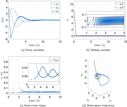
In this section, in order to show the properties of the proposed control scheme, an illustrative example is briefly discussed. Consider the following uncertain nonlinear system: (39) $\begin{array}{rl}{\dot{x}}_1& =x_2,\\ {\dot{x}}_2& =x_3,\\ {\dot{x}}_3& =0.1e^{-\mid x_2\mid \cdot t}\sin \left(x_1\right)+(1+0.1\sin (x_2\left)\right)(u+w).\end{array}$(39) Let $t_0$ be equal to 0, and the initial condition be $x\left(0\right)=[134{]}^{\mathrm{T}}$. Then, the system is stabilised by choosing the sliding variable as $\sigma =x_1+x_2+x_3$. In the triggering condition (6(6) $\mid \sigma \left(x\right(t\left)\right)\mid =\delta ,$(6) ) the threshold is $\delta =0.1$. The matched disturbance $w=-w^{sup}\sin \left(t\right)$, with $w^{sup}=2$. The control amplitude $U_{max}$ is selected equal to 15, while K=0.4, after a trial and error procedure to estimate the value of ${\mathrm{\Phi }}^{sup}=10$ and ${\mathrm{\Phi }}_{\delta }^{sup}=5$. Figure 2(a) shows the time evolution of the system state variables that are ultimately bounded in a vicinity of the system state space origin (see also Figure 2(d)). In Figure 2(b) the time evolution of the sliding variable in the presence of maximum time delay ${\mathrm{\Delta }}_{max}=0.0025$ s acting from t=0 s is shown. One can observe that, by selecting ${\delta }^{\prime }=0.06$ (see Theorem 4.8), even in the presence of maximum time delay and maximum uncertainty, σ is ultimately bounded with respect to the desired boundary layer ${\mathcal{B}}_{\delta }$. Finally, from Figure 2(c) one can appreciate that the inter-event times ${\tau }_k=t_{k+1}-t_k$ are always higher than the minimum inter-event time ${\tau }_{min}=0.007$ s (see Theorem 4.6). Moreover, considering a sampling time $T_s=1\times {10}^{-4}$ s, and a simulation time T=15 s the number of transmissions with the proposed ET-VSC is 99.6% less than the number required by the conventional (i.e. time-driven) SMC methodology. Note that, since the smart sensor works in continuous time, $T_s$ is chosen small enough so as to emulate a continuous time simulation setup. One can observe that reducing the width δ of the boundary layer ${\mathcal{B}}_{\delta }$ results in improving the convergence accuracy. Obviously, the correct balance between convergence accuracy and transmission load has to be searched depending on the specific application.

Figure 2. Time evolution of the state variables, sliding variable, inter-event times and the state space trajectory.

6. Conclusions

In this paper, an Event-Triggered Variable Structure Control scheme is presented. The main objective is to reduce the number of data transmissions over the network, while guaranteeing satisfactory performance. A triggering condition based on a suitably defined sliding variable and on a prescribed boundary layer of the sliding manifold is introduced. As a result, the ultimately boundedness of the solution of the controlled auxiliary system can be proved, which implies, under the considered assumptions, ultimately boundedness of the solution of the controlled system even in the presence of uncertainties and delayed transmissions. The proposed control scheme has the advantage of providing the way to get the desired balance between accuracy and transmission rate. In fact, the amplitude of the boundary layer, which is an ultimately positively invariant set, is a design parameter and the transmission rate is directly influenced by its choice. Moreover, the avoidance of the notorious Zeno behaviour is proved.

Disclosure statement

No potential conflict of interest was reported by the authors.

ORCID

Michele Cucuzzella http://orcid.org/0000-0003-1677-3289

Notes

1 The case in which the conventional assumptions on the knowledge of the uncertainty bounds are relaxed (Furtat, Orlov, & Fradkov, 2019) is left as an interesting future endeavour.

References

- Ames, A. D., Tabuada, P., & Sastry, S. (2006). On the stability of Zeno equilibria. In J. P. Hespanha and A. Tiwari (Eds.), Hybrid systems: Computation and control: 9th international workshop, HSCC 2006, Proceedings, Santa Barbara, CA, USA, March 29–31, 2006 (pp. 34–48). Berlin, Heidelberg: Springer.
- Aström, K. J. (2008). Event based control. In A. Astolfi and L. Marconi (Eds.), Analysis and design of nonlinear control systems (pp. 127–147). Berlin, Heidelberg: Springer.
- Behera, A. K., & Bandyopadhyay, B. (2016). Event-triggered sliding mode control for a class of nonlinear systems. International Journal of Control, 89(9), 1916–1931. doi: 10.1080/00207179.2016.1142617
- Behera, A. K., & Bandyopadhyay, B. (2017). Robust sliding mode control: An event-triggering approach. IEEE Transactions on Circuits and Systems II: Express Briefs, 64(2), 146–150. doi: 10.1109/TCSII.2016.2551542
- Behera, A. K., Bandyopadhyay, B., Xavier, N., & Kamal, S. (2015). Event-triggered sliding mode control for robust stabilization of linear multivariable systems. In X. Yu and M. Önder Efe (Eds.), Recent advances in sliding modes: From control to intelligent mechatronics (pp. 155–175). Cham: Springer International Publishing.
- Cucuzzella, M., & Ferrara, A. (2016). Event-triggered second order sliding mode control of nonlinear uncertain systems. Proceedings of European control conference (pp. 295–300), Aalborg, Denmark.
- Cucuzzella, M., & Ferrara, A. (2018). Practical second order sliding modes in single-loop networked control of nonlinear systems. Automatica, 89, 235–240. doi: 10.1016/j.automatica.2017.11.034
- Cucuzzella, M., Incremona, G. P., & Ferrara, A.2016). Event-triggered sliding mode control algorithms for a class of uncertain nonlinear systems: Experimental assessment. Proceedings of the American control conference (pp. 6549–6554).
- De Persis, C., Sailer, R., & Wirth, F. (2013). Parsimonious event-triggered distributed control: A Zeno free approach. Automatica, 49(7), 2116–2124. doi: 10.1016/j.automatica.2013.03.003
- De Persis, C., & Tesi, P. (2015). Input-to-state stabilizing control under denial-of-service. IEEE Transactions on Automatic Control, 60(11), 2930–2944. doi: 10.1109/TAC.2015.2416924
- Edwards, C., & Spurgen, S. K. (1998). Sliding mode control: Theory and applications. London: Taylor and Francis.
- Ferrara, A., & Cucuzzella, M. (2018). Event-triggered sliding mode control strategies for a class of nonlinear uncertain systems. In J. B. Clempner and W. Yu (Eds.), New perspectives and applications of modern control theory: In honor of Alexander S. Poznyak (pp. 397–425). Cham: Springer International Publishing.
- Ferrara, A., Sacone, S., & Siri, S. (2015a). Event-triggered model predictive schemes for freeway traffic control. Transportation Research Part C: Emerging Technologies, 58(Part C), 554–567. doi: 10.1016/j.trc.2015.01.020
- Ferrara, A., Sacone, S., & Siri, S. (2015b). Model-based event-triggered control for freeway traffic systems. Proceedings of the event-based control communication and signal processing international conference (pp. 1–6), Krakow, Poland.
- Fradkov, A., Miroshnik, I., & Nikiforov, V. (1999). Nonlinear and adaptive control of complex systems. Dordrecht: Kluwer Academic Publishers.
- Furtat, I., Orlov, Y., & Fradkov, A. (2019). Finite-time sliding mode stabilization using dirty differentiation and disturbance compensation. International Journal of Robust and Nonlinear Control, 29(3), 793–809. doi: 10.1002/rnc.4273
- Garcia, E., & Antsaklis, P. (2011). Model-based event-triggered control with time-varying network delays. Proceedings of the 16th 50th IEEE conference on decision control (pp. 1650–1655), Orlando, FL, USA.
- Heemels, W. P. M. H., Sandee, J. H., & Van Den Bosch, P. P. J. (2008). Analysis of event-driven controllers for linear systems. International Journal of Control, 81(4), 571–590. doi: 10.1080/00207170701506919
- Hespanha, J. P., Naghshtabrizi, P., & Xu, Y. (2007). A survey of recent results in networked control systems. Proceedings of the IEEE, 95(1), 138–162. doi: 10.1109/JPROC.2006.887288
- Incremona, G. P., & Ferrara, A. (2016). Adaptive model-based event-triggered sliding mode control. International Journal of Adaptive Control and Signal Processing, 30(8–10), 1298–1316.
- Incremona, G. P., Ferrara, A., & Magni, L. (2017). Asynchronous networked MPC with ISM for uncertain nonlinear systems. IEEE Transactions on Automatic Control, 62(9), 4305–4317. doi: 10.1109/TAC.2017.2653760
- Johansson, K. H., Lygeros, J., Sastry, S., & Egerstedt, M. (1999). Simulation of Zeno hybrid automata. Proceedings of the 16th 38th IEEE conference on decision control (pp. 3538–3543), Phoenix, AZ, USA.
- Leonov, G., Nijmeijer, H., Pogromsky, A., & Fradkov, A. (2010). Dynamics and control of hybrid mechanical systems. Singapore: World Scientific.
- Liberzon, D. (2003). Switching in systems and control. New York: Springer Science & Business Media.
- Montestruque, L. A., & Antsaklis, P. (2004). Stability of model-based networked control systems with time-varying transmission times. Proceedings of the American control conference (Vol. 49, pp. 1562–1572), Boston, MA, USA.
- Orlov, Y., & Utkin, V. I. (1998). Unit sliding mode control in infinite dimensional systems. Applied Mathematics and Computer Science, 8(1), 7–20.
- Ryvkin, S., & Palomar Lever, E. (2011). Sliding mode control for synchronous electric drives. London: CRC Press.
- Tabuada, P. (2007). Event-triggered real-time scheduling of stabilizing control tasks. IEEE Transactions on Automatic Control, 52(9), 1680–1685. doi: 10.1109/TAC.2007.904277
- Tan, S.-C., Lai, Y.-M., & Tse, C.-K. (2017). Sliding mode control of switching power converters: Techniques and implementation. London: CRC Press.
- Utkin, V. I. (1992). Sliding modes in control and optimization. New York: Springer-Verlag.
- Utkin, V. I. (1994). Sliding modes control in discrete-time and difference systems. Variable structure and Lyapunov control (Vol. 193, pp. 87–107). Berlin, Heidelberg: Springer.
- van der Schaft, A., & Schumacher, H. (2000). An introduction to hybrid dynamical systems (Vol. 251). London: Springer-Verlag.
- Wang, F., & Liu, D. (2008). Networked control systems: Theory and applications. London: Springer-Verlag London Limited.
- You, K.-Y., & Xie, L.-H. (2013). Survey of recent progress in networked control systems. Acta Automatica Sinica, 39(2), 101–117. doi: 10.1016/S1874-1029(13)60013-0
- Yu, H., & Antsaklis, P. (2011). Event-triggered real-time scheduling for stabilization of passive and output feedback passive systems. Proceedings of the American control conference (pp. 1674–1679), San Francisco, CA, USA.
- Yu, L., Barbot, J.-P., Benmerzouk, D., Boutat, D., Floquet, T., & Zheng, G. (2012). Discussion about sliding mode algorithms, Zeno phenomena and observability. In L. Fridman, J. Moreno, & R. Iriarte (Eds.), Lecture notes in control and information sciences (Vol. 412). Berlin: Springer.