A shift in paradigm for system identification

ABSTRACT

System identification is a mature research area with well established paradigms, mostly based on classical statistical methods. Recently, there has been considerable interest in so called kernel-based regularisation methods applied to system identification problem. The recent literature on this is extensive and at times difficult to digest. The purpose of this contribution is to provide an accessible account of the main ideas and results of kernel-based regularisation methods for system identification. The focus is to assess the impact of these new techniques on the field and traditional paradigms.

KEYWORDS:

• System identification
• linear regressions
• bias-variance tradeoff
• regularisation
• kernel methods

1. Introduction

System identification – to estimate models of dynamical systems from observed input-output data – has been around for more than half a century, with the term coined in Zadeh (1956). Many articles and textbooks on the topic have been written, e.g. Ljung (1999), Söderström and Stoica (1983) and Pintelon and Schoukens (2001). A certain state-of-the art paradigm has emerged, as described in Section 2.

Less than 10 years ago, an alternative approach, called kernel-based identification, with inspiration from machine learning, was described by Pillonetto and De Nicolao (2010). This approach gained considerable attention and during the past years the methods have been further developed in more than a hundred scientific papers, many with quite technical and sophisticated contents.

It is the purpose of the present contribution to give an accessible account of the main ideas and results of this approach with a focus on what it means for the paradigm and practical use of System Identification.

2. The traditional system identification setup

In the state-of the art paradigm of system identification, e.g. Ljung (1999), a parameterised model structure (1) $\mathcal{M}=\left\{\mathcal{M}\right(\theta )|\theta \in D_{\mathcal{M}}\}$(1) is defined, where each model $\mathcal{M}\left(\theta \right)$ provides a one-step-ahead predictor of the next output: $\hat{y}\left(t|\theta \right)$. Here θ is the parameter to be estimated, which ranges over a set of values $D_{\mathcal{M}}$. In this contribution all signals are assumed to take real values. The model structures can be of many different kinds: for linear black box models the state-space model structure of a given order n is a common choice as are several kinds of polynominal models, ARX, ARMAX, Output Error (OE), Box–Jenkins (BJ) models with given orders of the polynomials that define the respective structure, like See, for example, Ljung (1999), Ch 4. The model parameters θ are estimated by Maximum Likelihood (prediction error) methods, (ML/PEM), minimising sums of the prediction errors like: (2) $\hat{\theta }=\arg {\min }_{\theta \in D_{\mathcal{M}}}\sum _{t=1}^N\parallel y\left(t\right)-\hat{y}\left(t|\theta \right){\parallel }^2.$(2) The structural parameters, i.e. the model orders of polynomials and state are estimated by a separate procedure, like cross validation, or some order criterion like the Akaike Information Criterion, AIC, or the Bayesian order criterion, BIC.

This state-of the art procedure is supported by efficient software, and has been very successful, with many important practical applications.

3. Bias and variance

The goal of system identification is to provide as accurate a model as possible. There are two sources of errors in an estimated model $\mathcal{M}\left(\hat{\theta }\right)$:

Bias

The model class $\mathcal{M}$ was not big enough to contain a description of the true system. Then regardless of the amount and quality of the data, a correct model cannot be obtained. The distance between the true system and the best model in the model class is a bias error in the model estimate. It is deterministic in nature and does not depend on disturbances in the observed data.

Variance

The measured data is always corrupted by noise and disturbances and they will also affect the estimates. Even if a true model description is available in the model set, there will be a discrepancy between that and the estimate, caused by the disturbances. This error is stochastic in nature and called the variance error.

The total discrepancy between the true system and the model estimate will contain both these error components. The resulting mean square error, MSE is, conceptually (3) $MSE=BIA{S}^2+VARIANCE.$(3) So, in order to minimise the MSE one must take both components into consideration. The best choice is a trade-off in model flexibility: A large, flexible model set more easily accommodate any system; hence BIAS decreases with increased flexibility. On the other hand, a large model will have many parameters and is more vulnerable to be ‘fooled’ by disturbances in data. Hence VARIANCE will increase with increased model flexibility.

This BIAS-VARIANCE trade-off in selecting useful model flexibility is at the heart of all estimation problems and in the traditional system identification set-up it is performed when selecting the model order(s), typically by choosing one or several integers.

4. Linear regressions

A very common estimation structure is the Linear Regression, where the entity to be explained, the system output y in the case of system identification, is expressed as a linear combination of measured variables ϕ, plus a noise contribution e: (4) $y\left(t\right)={\varphi }^T\left(t\right)\theta +e\left(t\right),t=1,\dots ,N.$(4) Forming matrices $Y_N$ and ${\mathrm{\Phi }}_N$ by stacking $y\left(t\right)$ and $\varphi \left(t\right),t=1,\dots ,N$, this equation can be rewritten (5) $Y_N={\mathrm{\Phi }}_N\theta +E_N.$(5) Such a structure fits the common ARX-model (6) $\begin{array}{rl}& y\left(t\right)+a_{1}y(t-1)+\cdots +a_{n_a}y(t-n_a)\\ & =b_{1}u(t-1)+\cdots +b_{n_b}u(t-n_b)+e\left(t\right)\end{array}$(6) by taking (7) $\begin{array}{rl}\theta & =[\begin{array}{cccccc}{a}_1& \dots & a_{n_a}& b_1& \dots & b_{n_b}\end{array}{]}^{\mathrm{T}}\\ \varphi \left(t\right)& =[-y(t-1)\dots -y(t-n_a)\\ & u(t-1)\dots u(t-n_b){]}^{\mathrm{T}}.\end{array}$(7) The special case of $n_a=0$ is known as an FIR $($Finite Impulse Response$)$ model.

Many other identification problems can be formulated as a linear regression. In networked systems, for example, a potential node can be modelled by several incoming inputs from d other nodes (8) $y\left(t\right)=\sum _{i=1}^d{G}_i\left(q\right)u_i\left(t\right)+e\left(t\right).$(8) If each of the incoming transfer functions is modelled as a FIR model, it is clear how to form a linear regression (4(4) $y\left(t\right)={\varphi }^T\left(t\right)\theta +e\left(t\right),t=1,\dots ,N.$(4) ) analogously to (7(7) $\begin{array}{rl}\theta & =[\begin{array}{cccccc}{a}_1& \dots & a_{n_a}& b_1& \dots & b_{n_b}\end{array}{]}^{\mathrm{T}}\\ \varphi \left(t\right)& =[-y(t-1)\dots -y(t-n_a)\\ & u(t-1)\dots u(t-n_b){]}^{\mathrm{T}}.\end{array}$(7) ). The structure of the network will then be determined by finding out which $G_i$ can be set to zero. Such an application to sparse dynamic network identification is described in Chiuso and Pillonetto (2012), Chen, Andersen, Ljung, Chiuso, and Pillonetto (2014) as well as in Zorzi and Chiuso (2017)

A nonlinear regression model, $y\left(t\right)=g\left(\varphi \right(t\left)\right)+e\left(t\right)$ can be dealt with as a linear regression if a function expansion in predetermined basis functions $g_k$ is used: (9) $g\left(\varphi \right)=\sum _{k=1}^d{\alpha }_k{g}_k\left(\varphi \right).$(9) The model will then become a linear regression in the parameters α with $g_k\left(\varphi \right(t\left)\right)$ as the known regressors. See, for example, Chiuso and Pillonetto (2012) and Pan, Yuan, Ljung, Goncalves, and Stan (2017) for such an application.

The great advantage with a linear regression is that the parameters can readily be estimated by the linear least squares method: (10) $\begin{array}{rl}{\hat{\theta }}_N^{LS}& =\arg {\min }_{\theta }\parallel Y_N-{\mathrm{\Phi }}_N\theta {\parallel }^2\\ & =({\mathrm{\Phi }}_N^T{\mathrm{\Phi }}_N{)}^{-1}{\mathrm{\Phi }}_N^T{Y}_N\\ & =R_N^{-1}{F}_N,\end{array}$(10) where $R_N={\mathrm{\Phi }}_N^T{\mathrm{\Phi }}_N,F_N={\mathrm{\Phi }}_N^T{Y}_N$.

5. Regularisation

It is well known that if indeed the system is described by (4(4) $y\left(t\right)={\varphi }^T\left(t\right)\theta +e\left(t\right),t=1,\dots ,N.$(4) ) for a certain ‘true’ parameter ${\theta }_0$ and white Gaussian noise e with variance ${\sigma }^2$, then the LS estimate (10(10) $\begin{array}{rl}{\hat{\theta }}_N^{LS}& =\arg {\min }_{\theta }\parallel Y_N-{\mathrm{\Phi }}_N\theta {\parallel }^2\\ & =({\mathrm{\Phi }}_N^T{\mathrm{\Phi }}_N{)}^{-1}{\mathrm{\Phi }}_N^T{Y}_N\\ & =R_N^{-1}{F}_N,\end{array}$(10) ) is the Maximum Likelihood estimate, and it will be unbiased, (11) $E{\hat{\theta }}_N^{LS}={\theta }_0$(11) with variance (12) $E({\hat{\theta }}_N^{LS}-{\theta }_0)({\hat{\theta }}_N^{LS}-{\theta }_0{)}^{\mathrm{T}}={\sigma }^2{R}_N^{-1}.$(12) This variance is the Cramer–Rao bound, the smallest variance that can be achieved in any unbiased estimator.

In the least squares solution (10(10) $\begin{array}{rl}{\hat{\theta }}_N^{LS}& =\arg {\min }_{\theta }\parallel Y_N-{\mathrm{\Phi }}_N\theta {\parallel }^2\\ & =({\mathrm{\Phi }}_N^T{\mathrm{\Phi }}_N{)}^{-1}{\mathrm{\Phi }}_N^T{Y}_N\\ & =R_N^{-1}{F}_N,\end{array}$(10) ) it may happen that the matrix $R_N$ is ill-conditioned. For that reason, Regularisation has been suggested, see Tikhonov and Arsenin (1977) for a general treatment of regularisation. This is generally expressed in optimisation form as (13) $\begin{array}{rl}{\hat{\theta }}_N^R\left(\mathrm{\Pi }\right)& =\arg \min \parallel Y_N-\mathrm{\Phi }{}_N\theta {\parallel }^2+{\sigma }^2{\theta }^T{\mathrm{\Pi }}^{-1}\theta \\ & =[R_N+{\sigma }^2{\mathrm{\Pi }}^{-1}{]}^{-1}{\mathrm{\Phi }}_N^T{Y}_N.\end{array}$(13) With Π being a suitable positive definite matrix, this will improve the conditioning of the matrix to be inverted. This numerical aspect was an original reason for regularisation.

In a Bayesian setting, where θ is seen as a random vector, one may note that (13(13) $\begin{array}{rl}{\hat{\theta }}_N^R\left(\mathrm{\Pi }\right)& =\arg \min \parallel Y_N-\mathrm{\Phi }{}_N\theta {\parallel }^2+{\sigma }^2{\theta }^T{\mathrm{\Pi }}^{-1}\theta \\ & =[R_N+{\sigma }^2{\mathrm{\Pi }}^{-1}{]}^{-1}{\mathrm{\Phi }}_N^T{Y}_N.\end{array}$(13) ) actually defines the MAP: Maximum a Posteriori estimate of θ in case there is prior information that the prior distribution of θ is Gaussian with zero mean and covariance matrix Π.

Back to a ‘classical’ perspective, where ${\theta }_0$ is unknown but fixed parameter, the statistical properties of the regularised estimate ${\hat{\theta }}_N^R\left(\mathrm{\Pi }\right)$ can easily be determined. It will no longer be unbiased: (14) ${\hat{\theta }}_{bias}^R=E{\hat{\theta }}_N^R\left(\mathrm{\Pi }\right)-{\theta }_0=-(R_N+{\sigma }^2{\mathrm{\Pi }}^{-1}{)}^{-1}{\sigma }^2{\mathrm{\Pi }}^{-1}{\theta }_0$(14) and the variance around the mean will be (15) ${\sigma }^2(R_N+{\sigma }^2{\mathrm{\Pi }}^{-1}{)}^{-1}{R}_N(R_N+{\sigma }^2{\mathrm{\Pi }}^{-1}{)}^{-1}.$(15) We realise that if $R_N$ is ill-conditioned, the Cramer–Rao bound, the best possible variance of an unbiased estimate could be extremely large. At the same time, even a small regularisation term, e.g. ${\mathrm{\Pi }}^{-1}=\delta I$ will improve the conditioning of the matrix $R_N+{\sigma }^2{\mathrm{\Pi }}^{-1}$ and hence the parameter variance considerably.

The small regularisation will also introduce a small bias, but the combined effect on the MSE, see Section 3, could be very beneficial.

This regularisation, with a scaled identity matrix has long been used in statistics under the name of ridge regression.

For the regularised estimate, the mean square error (MSE) of the estimate is (16) $\begin{array}{rl}& E\left[\right({\hat{\theta }}_N-{\theta }_0\left)\right({\hat{\theta }}_N-{\theta }_0{)}^{\mathrm{T}}]=(R_N+{\mathrm{\Pi }}^{-1}{)}^{-1}\\ & \times ({\sigma }^2{R}_N+{\mathrm{\Pi }}^{-1}{\theta }_0{\theta }_0^T{\mathrm{\Pi }}^{-1})(R_N+{\mathrm{\Pi }}^{-1}{)}^{-1}.\end{array}$(16) A rational choice of Π is one that makes this MSE matrix small. How shall we think of good such choices? It is useful to first establish the following Lemma of algebraic nature

Lemma 5.1

Consider the matrix (17) $M\left(Q\right)=(QR+I{)}^{-1}(QRQ+Z\left)\right(RQ+I{)}^{-1},$(17) where I is the identity matrix with suitable dimension, Q,R and Z are positive semidefinite matrices. Then for all Q (18) $M\left(Q\right)\ge M\left(Z\right),$(18) where the inequality is in matrix sense.

The proof consists of straightforward calculations, see, e.g. Chen, Ohlsson, and Ljung (2012).

So, the question what P gives the best MSE of the regularised estimate has a clear answer: Use (19) $\mathrm{\Pi }={\theta }_0{\theta }_0^T.$(19) Not surprisingly the best regularisation depends on the unknown system.

Regularisation will thus be a crucial instrument for dealing with the core problem of bias-variance trade-off. Next we illustrate the idea on a simple model example.

6. Example: finite impulse response estimation

Consider the problem to estimate the impulse response of a linear system as an FIR model: (20) $y\left(t\right)=\sum _{k=0}^{n_b}g\left(k\right)u(t-k)+e\left(t\right).$(20) The choice of order $n_b$ presents a trade-off between bias (large $n_b$ is required to capture slowly decaying impulse responses without too much error) and variance (large $n_b$ gives many parameters to estimate which gives large variance).

Let us illustrate it with a simulated example. We pick a simple second-order butterworth filter as the system: (21) $G\left(z\right)=\frac{0.02008+0.04017z^{-1}+0.02008z^{-2}}{1-1.561z^{-1}+0.6414z^{-2}}.$(21) Its impulse response is shown in Figure 1.

Figure 1. The true impulse response.

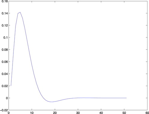
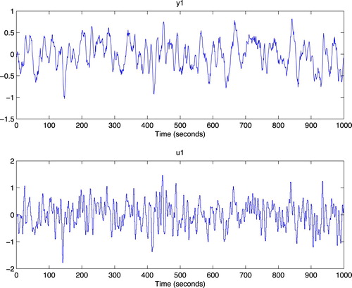
It has decayed to zero after less than 50 time steps. Let us estimate it from data generated by the system. We simulate the system with low-pass filtered white noise as input and add a small white noise output disturbance with variance 0.0025 to the output. One thousand samples are collected. The data is shown in Figure 2.

Figure 2. The data used for estimation.

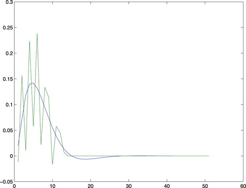
To determine a good value for $n_b$ we basically have to try a few values and by some validation procedure evaluate which is best. That can be done in several ways, but since we know the true system in this case, we can determine the theoretically best possible value, by trying out all models with $n_b=1,\dots ,50$ and find which one has the best fit to the true impulse response. Such a test shows that $n_b=13$ gives the best error norm (mean square error (MSE)=0.2522). This estimated impulse response is shown together with the true one in Figure 3.Despite the 1000 data points, with very good signal to noise ratio the estimate is not impressive. The reason is that the low pass input has poor excitation.

Figure 3. The true impulse response together with the estimate for order nb=13.

Let us therefore try to reach a good bias-variance trade-off by ridge regression for an FIR model of order 50. That is we use $\mathrm{\Pi }=I$ (identity) in (13(13) $\begin{array}{rl}{\hat{\theta }}_N^R\left(\mathrm{\Pi }\right)& =\arg \min \parallel Y_N-\mathrm{\Phi }{}_N\theta {\parallel }^2+{\sigma }^2{\theta }^T{\mathrm{\Pi }}^{-1}\theta \\ & =[R_N+{\sigma }^2{\mathrm{\Pi }}^{-1}{]}^{-1}{\mathrm{\Phi }}_N^T{Y}_N.\end{array}$(13) ). The resulting estimate has an MSE error norm of 0.1171 to the true impulse response and is shown in Figure 4.

Figure 4. The true impulse response together with the ridge-regularised estimate for order nb=50.

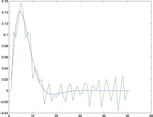
Clearly even this simple choice of regularisation gives a much better bias–variance tradeoff, than selecting FIR order.

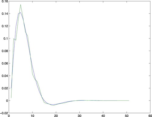
By using the insight that the true impulse response decays to zero and is smooth, we can tailor the choice of Π to the data using the methods to be described in Sections 8 and 9, and obtain the estimate shown in Figure 5 with an MSE norm of 0.0461.

Figure 5. The true impulse response together with the tuned regularised estimate for order nb=50.

Input design is another important isssue to improve the estimation accuracy of the kernel-based regularisation methods. A two-step procedure is proposed in Mu and Chen (2018), where in the first step, a quadratic transformation of the input is constructed such that the transformed input design problems are convex and their global minima can be found efficiently by applying well-developed convex optimisation software package and in the second step, an expression is derived for the optimal input based on the global minima found in the first step by solving the inverse image of the quadratic transformation.

7. The two choices

The treatment of regularisation in Section 5 is valid for any linear regression problem. In a sense, the optimal regularisation (for smallest MSE) is known as (19(19) $\mathrm{\Pi }={\theta }_0{\theta }_0^T.$(19) ), but this choice depends on the true system and cannot be used in practice. So we have to focus on how to choose Π. It is convenient to split this choice into two parts.

kernel

The choice of the structure of Π, that is a parameterisation of the matrix $\mathrm{\Pi }\left(\eta \right)$. For reasons that will be clear in Section 8, this matrix is also called the kernel of the estimation problem. That involves consideration of the actual estimation problem: what is the nature of θ, what properties can be expected.

tuning

Once the kernel structure $\mathrm{\Pi }\left(\eta \right)$ has been selected, the problem is to estimate the hyperparameters $\eta \in D_{\eta }$ using the available observations. This problem as such is a pure estimation problem of statistical nature and does not depend on the actual system.

8. Kernel structure

In this section we assume that the linear regression actually is to estimate the system's impulse response as an FIR model (20(20) $y\left(t\right)=\sum _{k=0}^{n_b}g\left(k\right)u(t-k)+e\left(t\right).$(20) ). That is, the linear regression as in (6(6) $\begin{array}{rl}& y\left(t\right)+a_{1}y(t-1)+\cdots +a_{n_a}y(t-n_a)\\ & =b_{1}u(t-1)+\cdots +b_{n_b}u(t-n_b)+e\left(t\right)\end{array}$(6) ) with $n_a=0$.That makes the true parameter ${\theta }_0$ equal to the true impulse response $g^0\left(k\right)$.

The kernels for regularisation really have their roots in (continuous) function estimation/approximation techniques, see e.g. Wahba (1999). Using Reproducing Kernel Hilbert Space, (RKHS) theory, 'basis functions' defined by splines appeared as natural and useful elements for function approximation. They define what are called the kernels for the function estimation. In our discrete time linear regression formulation, the kernel functions correspond to the Π matrix.

In system identification, the kernel design plays a similar role as the model structure design for ML/PEM and determines the underlying model structure for kernel-based regularisation methods. In the past few years, many efforts have been spent on this issue and many kernels have been invented to embed various types of prior knowledge, e.g. Pillonetto and De Nicolao (2010), Pillonetto, Chiuso, and De Nicolao (2011), Chen et al. (2014, 2016, 2012), Dinuzzo (2015), Carli, Chen, and Ljung (2017), Marconato, Schoukens, and Schoukens (2016), Zorzi and Chiuso (2018), and Pillonetto, Chen, Chiuso, De Nicolao, and Ljung (2016). Among those kernels, the so-called stable spline (SS) kernel Pillonetto and De Nicolao (2010), and diagonal correlated (DC) kernel Pillonetto et al. (2011) are widely recognised and used in the system identification community.

1. In Pillonetto and De Nicolao (2010) the SS kernel is derived by applying a wrapping technique to the second-order spline kernel that is used in continuous function estimation. More specifically, the second-order spline kernel $B(s,s^{\prime })$ is defined on [0,1] × [0,1] and its variance is increasing from 0 to 1 and the corresponding ‘stable spline’ kernel is defined as $B({\mathrm{e}}^{-\beta t},{\mathrm{e}}^{-\beta t^{\prime }})$ with $t,t^{\prime }\in [0,\mathrm{\infty })$. This leads to the SS kernel, which takes the following form: The regularisation matrix $\mathrm{\Pi }\left(\eta \right)$ has the $k,\ell$ element (22) $C\left({\lambda }^{k+\ell +max(k,\ell )}-\frac{1}{3}{\lambda }^{3max(k,\ell )}\right),$(22) where $\eta =[C,\lambda ]$ with C>0 and $0<\lambda <1$ are the hyperparameters. Similar idea has also been used to derive the first-order stable spline kernel, Pillonetto, Chiuso, and De Nicolao (2010) which takes the following form, (23) $C{\lambda }^{max(k,\ell )}.$(23) 2. In Chen et al. (2012) the DC kernel is derived by mimicking the behaviour of the optimal kernel, which is $g^0\left(t\right)g^0\left(t^{\prime }\right)$ with $g^0\left(t\right)$ being the true impulse response of the system to be identified (cf (19(19) $\mathrm{\Pi }={\theta }_0{\theta }_0^T.$(19) )). More specifically, since $g^0\left(t\right)$ decays to zero exponentially, it is natural to let the variance of the DC kernel decays with a factor, say λ; since the impulse response is smooth, it is also natural to let the neighbouring impulse response coefficients highly correlated, say with the correlation coefficient ρ. This leads to the DC kernel, which takes the following form, (24) $C{\lambda }^{(k+\ell )/2}{\rho }^{|k-\ell |},$(24) where $\eta =[C,\lambda ,\rho ]$, with $C>0,0<\lambda <,|\rho |\le 1$ are the hyperparameters. An interesting special case is to take $\rho =\sqrt{\lambda }$. This is called the TC Kernel in Chen et al. (2012), the tuned correlation kernel. Note that in this case the expressions  (23(23) $C{\lambda }^{max(k,\ell )}.$(23) ) and (24(24) $C{\lambda }^{(k+\ell )/2}{\rho }^{|k-\ell |},$(24) ) coincide. This shows the close relationship between the two approaches.This kernel was the one used in Figure 5.

The SS and DC/TC kernels are derived based on heuristic ideas. In practice, we need to develop systematic ways to design kernels to embed various types of prior knowledge. Interestingly, Chen (2018), finds that the SS and DC kernels share some common properties and has developed, based on this finding, two systematic ways of kernel design methods: one is from a machine learning perspective and the other one is from a system theory perspective.

1. Machine Learning perspective: If the impulse response is treated as a function and the prior knowledge is about its decay and varying rate, then the amplitude modulated locally stationary (AMLS) kernel can be designed: a rank-1 kernel and a stationary kernel are used to account for the decay and varying rate of the impulse response, respectively.

2. System Theory perspective: Suppose that the system's impulse is associated with an LTI system and the prior knowledge is that the LTI system is stable and may be overdamped, underdamped, has multiple distinct time constants or multiple distinct resonant frequencies, etc. Then a simulation induced (SI) kernel can be designed by a nominal model that embeds the given prior knowledge. Also, a multiplicative uncertainty configuration is used to take into account both the nominal model and its uncertainty, and the model is simulated with an impulsive input to get the SI kernel.

9. Hyperparameter tuning

The hyperparameter estimation plays a similar role as the model order selection in ML/PEM and its essence is to determine a suitable model complexity based on the data. As mentioned in the survey of kernel regularisation methods, Pillonetto, Dinuzzo, Chen, De Nicolao, and Ljung (2014), many methods can be used for hyperparameter estimation, such as the cross-validation (CV), empirical Bayes (EB), $C_p$ statistics and Stein's unbiased risk estimator (SURE), etc. Hyperparameter estimation is discussed in, e.g. Chen et al. (2014), Aravkin, Burke, Chiuso, and Pillonetto (2012a, 2012b, 2014), Pillonetto and Chiuso (2015), Mu, Chen, and Ljung (2017), and Mu, Chen, and Ljung (2018).

We now consider the problem to estimate the hyperparameter $\eta \in D_{\eta }$ in any kernel structure $\mathrm{\Pi }\left(\eta \right)$ for any linear regression problem (13(13) $\begin{array}{rl}{\hat{\theta }}_N^R\left(\mathrm{\Pi }\right)& =\arg \min \parallel Y_N-\mathrm{\Phi }{}_N\theta {\parallel }^2+{\sigma }^2{\theta }^T{\mathrm{\Pi }}^{-1}\theta \\ & =[R_N+{\sigma }^2{\mathrm{\Pi }}^{-1}{]}^{-1}{\mathrm{\Phi }}_N^T{Y}_N.\end{array}$(13) ). As pointed out in Pillonetto and Chiuso (2015) the problem of hyperparameter estimation has certain links with the order selection (tuning complexity) problem. What would be the goal of the estimate? In traditional estimation one seeks estimates, that at least when data sample record tends to infinity converge to the ‘true’ parameters. What is the ‘true’ hyperparameter for the current problem?

If we know the true system ${\theta }_0$, we can for any Π in (13(13) $\begin{array}{rl}{\hat{\theta }}_N^R\left(\mathrm{\Pi }\right)& =\arg \min \parallel Y_N-\mathrm{\Phi }{}_N\theta {\parallel }^2+{\sigma }^2{\theta }^T{\mathrm{\Pi }}^{-1}\theta \\ & =[R_N+{\sigma }^2{\mathrm{\Pi }}^{-1}{]}^{-1}{\mathrm{\Phi }}_N^T{Y}_N.\end{array}$(13) ) evaluate the MSE (25) $MS{E}_N\left(\eta \right)=E\parallel {\hat{\theta }}_N^R\left(\mathrm{\Pi }\right(\eta \left)\right)-{\theta }_0{\parallel }^2.$(25) We would like to find an η so that this MSE is minimised asymptotically as $N\to \mathrm{\infty }$. A complication is that $MS{E}_N\left(\eta \right)$ will tend to zero for all η. We therefore look at the rate by which the error tends to the Cramer-Rao limit: (26) $\begin{array}{rl}W(P,\mathrm{\Sigma },{\theta }_0)& =\underset{N\to \mathrm{\infty }}{lim}{N}^2\left(MS{E}_N\right(\eta )-{\sigma }^2\mathrm{Tr}({\mathrm{\Sigma }}^{-1}\left)\right)\\ & ={\sigma }^4{\theta }_0^T{\mathrm{\Pi }}^{-1}{\mathrm{\Sigma }}^{-2}{\mathrm{\Pi }}^{-1}{\theta }_0-2{\sigma }^4\mathrm{Tr}({\mathrm{\Sigma }}^{-1}{\mathrm{\Pi }}^{-1}{\mathrm{\Sigma }}^{-1})\end{array}$(26) (27) $\begin{array}{rl}\mathrm{\Sigma }& =\underset{N\to \mathrm{\infty }}{lim}\frac{1}{N}{\mathrm{\Phi }}_N^T{\mathrm{\Phi }}_N.\end{array}$(27) Now the ‘optimal’ hyperparameter will be (28) ${\eta }^{\ast }(\mathrm{\Sigma },{\theta }_0)={\mathrm{argmin}}_{\eta \in D_{\eta }}W(\eta ,\mathrm{\Sigma },{\theta }_0).$(28) It depends both on the true system ${\theta }_0$ and the data Σ.

Remark: Regularisation is essentially a transient phenomenon. As $N\to \mathrm{\infty }$ the effect disappears for any η. Still it is meaningful to use the asymptotically defined ${\eta }^{\ast }$, since it is a well defined value, and even for large N it gives the best possible MSE.

We would like to optimally estimate η. For the linear regression case with a Gaussian prior for θ we have (29) $Y=\mathrm{\Phi }\theta +E,\theta \in N(0,\mathrm{\Pi }(\eta \left)\right).$(29) If E is Gaussian with covariance matrix ${\sigma }^{2}I$, Y will also be Gaussian with zero mean and covariance matrix (30) $Z\left(\eta \right)=\mathrm{\Phi \Pi }\left(\eta \right){\mathrm{\Phi }}^T+{\sigma }^{2}I.$(30) This means that the probability distribution of Y is known up to η which implies that parameter can be estimated by the maximum likelihood method as (31) ${\hat{\eta }}_N^{EB}=\arg {\min }_{\eta \in D_{\eta }}{Y}^{T}Z(\eta {)}^{-1}Y+\log detZ(\eta ).$(31) This estimate of the prior distribution is known as Empirical Bayes. It is a very natural and easy-to-use estimate and is probably the most commonly used one. It normally performs very well, but it is shown in Mu et al. (2018) that it in general does not obey ${\hat{\eta }}_N^{EB}\to {\eta }^{\ast }$ as $N\to \mathrm{\infty }$.

To achieve this goal it is necessary to form another criterion. In Pillonetto and Chiuso (2015) an SURE (Stein's Unbiased Risk Estimator) criterion aiming for minimising the MSE (25(25) $MS{E}_N\left(\eta \right)=E\parallel {\hat{\theta }}_N^R\left(\mathrm{\Pi }\right(\eta \left)\right)-{\theta }_0{\parallel }^2.$(25) ) was studied: (32) $\begin{array}{rl}{\mathcal{F}}_N\left(\eta \right)& =\parallel {\hat{\theta }}_N^{LS}-{\hat{\theta }}_N^R\left(\mathrm{\Pi }\right(\eta \left)\right){\parallel }^2+{\sigma }^2\left(2H^{-1}-({\mathrm{\Phi }}_N^T{\mathrm{\Phi }}_N{)}^{-1}\right)\\ H& ={\mathrm{\Phi }}_N^T{\mathrm{\Phi }}_N+{\sigma }^2{\mathrm{\Pi }}^{-1}\left(\eta \right)\end{array}$(32) with estimate (33) ${\hat{\eta }}_N^S=\arg {\min }_{\eta \in D\eta }{\mathcal{F}}_N\left(\eta \right).$(33) It is shown in Mu et al. (2018) that indeed (34) $\underset{N\to \mathrm{\infty }}{lim}{\hat{\eta }}_N^S={\eta }^{\ast }.$(34) The estimate is tested in simulations in Mu et al. (2018) and Pillonetto and Chiuso (2015). For well conditioned regressors it behaves well, but if ${\mathrm{\Phi }}_N^T{\mathrm{\Phi }}_N$ is ill-conditioned it suffers from numerical implementation problems.

10. General identification problems

So far we have only dealt with linear regressions (4(4) $y\left(t\right)={\varphi }^T\left(t\right)\theta +e\left(t\right),t=1,\dots ,N.$(4) ). They do cover many important estimation problems, but traditional system identification deals with many more models. Linear black-box models, (35) $y\left(t\right)=G\left(q\right)u\left(t\right)+H\left(q\right)e\left(t\right)$(35) form a very common class of models, where G and H can be parameterised in several different ways, ARMAX, Ouput-Error, Box-Jenkins or State-space models and estimated by tailored sophisticated identification algorithms.

It is an important and well known fact, Ljung and Wahlberg (1992), that any linear system (35(35) $y\left(t\right)=G\left(q\right)u\left(t\right)+H\left(q\right)e\left(t\right)$(35) ) can be arbitrarily well approximated by an ARX-model (6(6) $\begin{array}{rl}& y\left(t\right)+a_{1}y(t-1)+\cdots +a_{n_a}y(t-n_a)\\ & =b_{1}u(t-1)+\cdots +b_{n_b}u(t-n_b)+e\left(t\right)\end{array}$(6) ) with sufficiently large orders, (36) $y\left(t\right)=\frac{B\left(q\right)}{A\left(q\right)}u\left(t\right)+\frac{1}{A\left(q\right)}e\left(t\right).$(36) This is a linear regression, (7(7) $\begin{array}{rl}\theta & =[\begin{array}{cccccc}{a}_1& \dots & a_{n_a}& b_1& \dots & b_{n_b}\end{array}{]}^{\mathrm{T}}\\ \varphi \left(t\right)& =[-y(t-1)\dots -y(t-n_a)\\ & u(t-1)\dots u(t-n_b){]}^{\mathrm{T}}.\end{array}$(7) ). Thus the regularisation theory can readily be applied to estimate (36(36) $y\left(t\right)=\frac{B\left(q\right)}{A\left(q\right)}u\left(t\right)+\frac{1}{A\left(q\right)}e\left(t\right).$(36) ) and hence any linear black-box model.

The predictor can be written (cf (6(6) $\begin{array}{rl}& y\left(t\right)+a_{1}y(t-1)+\cdots +a_{n_a}y(t-n_a)\\ & =b_{1}u(t-1)+\cdots +b_{n_b}u(t-n_b)+e\left(t\right)\end{array}$(6) )) (37) $\begin{array}{rl}\hat{y}\left(t\right)& =-a_{1}y(t-1)-\cdots -a_{n_a}y(t-n_a)\end{array}$(37) (38) $\begin{array}{rl}& +b_{1}u(t-1)+\cdots +b_{n_b}u(t-n_b)\end{array}$(38) and can be seen as two impulse responses - one from y with the a-parameters and one from u with the b-parameters. Thus the thinking from Section 8 to form the regularisation matrix from impulse response properties can be applied also here.

How does it work? The survey Pillonetto et al. (2014) contains extensive studies with simulated and real data comparing regularised ARX-models with kernels like (24(24) $C{\lambda }^{(k+\ell )/2}{\rho }^{|k-\ell |},$(24) ) (applying different kernels to the input and output impulse responses in (7(7) $\begin{array}{rl}\theta & =[\begin{array}{cccccc}{a}_1& \dots & a_{n_a}& b_1& \dots & b_{n_b}\end{array}{]}^{\mathrm{T}}\\ \varphi \left(t\right)& =[-y(t-1)\dots -y(t-n_a)\\ & u(t-1)\dots u(t-n_b){]}^{\mathrm{T}}.\end{array}$(7) )) with the state-of-the art techniques for ARMAX and state-space models. The result is that the regularised estimates generally outperform the standard techniques. The weak spot with the conventional techniques is that it is difficult to find the best model orders. Even an oracle that picks the best possible orders (knowing the true system) in the conventional approach will not do as well as the regularisation. The reason clearly is that the tuning of continuous regularisation parameters – that allows ‘non-integer orders’ – is a more powerful tool and concept than picking integer order by some selection rule.

11. Conclusions

It is clear that regularisation techniques are a most useful addition to the toolbox of identification methods. The ‘automatic’ tuning of continuous hyperparameters that determine the flexibility of the used model structure is a powerful and versatile tool compared to the classical rules of selecting model orders. The paradigms in using identification techniques for black box linear systems should definitely allow considering regularisation techniques. In fact, Mathwork's System Identification Toolbox, Ljung, Singh, and Chen (2015) has recently included several of the regularisation techniques described in this contribution. The implementation details can be found in Chen and Ljung (2013).

Disclosure statement

No potential conflict of interest was reported by the authors.

ORCID

Lennart Ljung  http://orcid.org/0000-0003-4881-8955

Additional information

Funding

The work has been supported by the National Natural Science Foundation of China under the contracts No. 61603379 and. No. 61773329, the Thousand Youth Talents Plan funded by the central government of China, the Shenzhen Projects Ji-20170189 and Ji-20160207 funded by the Shenzhen Science and Technology Innovation Council, the Presidents grant under contract No. PF. 01.000249 and the Startup grant under contract No. 2014.0003.23 funded by the Chinese University of Hong Kong, Shenzhen, by Shenzhen Fundamental Research Fund under project No. ZDSYS201707251409055, and by a research grant for junior researchers under contract No. 2014-5894 funded by Swedish Research Council.

References

- Aravkin, A., Burke, J. V., Chiuso, A., & Pillonetto, G. (2012a). On the mse properties of empirical bayes methods for sparse estimation. In Proceeding of the IFAC symposium on system identification (pp. 965–970). Brussels, Belgium.
- Aravkin, A., Burke, J. V., Chiuso, A., & Pillonetto, G. (2012b). On the estimation of hyperparameters for empirical bayes estimators: Maximum marginal likelihood vs minimum mse. In Proceeding of the IFAC symposium on system identification (pp. 125–130). Brussels, Belgium.
- Aravkin, A., Burke, J. V., Chiuso, A., & Pillonetto, G. (2014). Convex vs non-convex estimators for regression and sparse estimation: The mean squared error properties of ard and glasso. Journal of Machine Learning Research, 15(1), 217–252.
- Carli, F. P., Chen, T., & Ljung, L. (2017, March). Maximum entropy kernels for system identification. IEEE Transactions on Automatic Control, 62, 1471–1477. doi: 10.1109/TAC.2016.2582642
- Chen, T. (2018). On kernel design for regularised lti system identification. Automatica, 90, 109–122. doi: 10.1016/j.automatica.2017.12.039
- Chen, T., Andersen, M. S., Ljung, L., Chiuso, A., & Pillonetto, G. (2014). System identification via sparse multiple kernel-based regularization using sequential convex optimization techniques. IEEE Transactions on Automatic Control, 59(11), 2933–2945. doi: 10.1109/TAC.2014.2351851
- Chen, T., Ardeshiri, T., Carli, F. P., Chiuso, A., Ljung, L., & Pillonetto, G. (2016). Maximum entropy properties of discrete-time first-order stable spline kernel. Automatica, 66, 34–38. doi: 10.1016/j.automatica.2015.12.009
- Chen, T., & Ljung, L. (2013). Implementation of algorithms for tuning parameters in regularized least squares problems in system identification. Automatica, 50, 2213–2220. doi: 10.1016/j.automatica.2013.03.030
- Chen, T., Ohlsson, H., & Ljung, L. (2012). On the estimation of transfer functions, regularizations and gaussian processes – revisited. Automatica, 48(8), 1525–1535. doi: 10.1016/j.automatica.2012.05.026
- Chiuso, A., & Pillonetto, G. (2012, April). A Bayesian approach to sparse dynamic network identification. Automatica, 48, 1107–1111. doi: 10.1016/j.automatica.2012.05.054
- Dinuzzo, F. (2015). Kernels for linear time invariant system identification. SIAM Journal on Control and Optimization, 53(5), 3299–3317. doi: 10.1137/130920319
- Ljung, L. (1999). System identification – theory for the user (2nd ed.). Upper Saddle River, NJ: Prentice-Hall.
- Ljung, L., Singh, R., & Chen, T. (2015, Oct). Regularization features in the system identification toolbox. In IFAC-PapersOnLine, vol. 48–28, IFAC Symposium on System Identification.
- Ljung, L., & Wahlberg, B. (1992). Asymptotic properties of the least-squares method for estimating transfer functions and disturbance spectra. Advances in Applied Probability, 24, 412–440. doi: 10.2307/1427698
- Marconato, A., Schoukens, M., & Schoukens, J. (2016). Filter-based regularisation for impulse response modelling. IET Control Theory & Applications, 11(2), 194–204. doi: 10.1049/iet-cta.2016.0908
- Mu, B., & Chen, T. (2018, November). On input design for regularized LTI system identifiction: Power constrained input. Automatica, 97, 327–338. doi: 10.1016/j.automatica.2018.08.010
- Mu, B., Chen, T., & Ljung, L. (2017). Tuning of hyperparameters for fir models – an asymptotic theory. In Proceedings of the 20th IFAC world congress (pp. 2818–2823) Toulouse, France.
- Mu, B., Chen, T., & Ljung, L. (2018). On asymptotic properties of hyperpa-rameter estimators for kernel-based regularization methods. Automatica, 94, 381–395. doi: 10.1016/j.automatica.2018.04.035
- Pan, W., Yuan, Y., Ljung, L., Goncalves, J., & Stan, G.-B. (2017). Identification of nonlinear state-space systems from heterogeneous datasets. IEEE Transactions Control of Network Systems, 5(2), 737–747. doi: 10.1109/TCNS.2017.2758966
- Pillonetto, G., Chen, T., Chiuso, A., De Nicolao, G., & Ljung, L. (2016). Regularized linear system identification using atomic, nuclear and kernel-based norms: The role of the stability constraint. Automatica, 69, 137–149. doi: 10.1016/j.automatica.2016.02.012
- Pillonetto, G., & Chiuso, A. (2015). Tuning complexity in regularized kernel-based regression and linear system identification: The robustness of the marginal likelihood estimator. Automatica, 58, 106–117. doi: 10.1016/j.automatica.2015.05.012
- Pillonetto, G., Chiuso, A., & De Nicolao, G. (2010). Regularized estimation of sums of exponentials in spaces generated by stable spline kernels. In Proc. 2010 American Control Conference (pp. 498–503). Baltimore, MD: Marriott Waterfront.
- Pillonetto, G., Chiuso, A., & De Nicolao, G. (2011). Prediction error identification of linear systems: A nonparametric gaussian regression approach. Automatica, 47(2), 291–305. doi: 10.1016/j.automatica.2010.11.004
- Pillonetto, G., & De Nicolao, G. (2010). A new kernel-based approach for linear system identification. Automatica, 46(1), 81–93. doi: 10.1016/j.automatica.2009.10.031
- Pillonetto, G., Dinuzzo, F., Chen, T., De Nicolao, G., & Ljung, L. (2014). Kernel methods in system identification, machine learning and function estimation: A survey. Automatica, 50(3), 657–682. doi: 10.1016/j.automatica.2014.01.001
- Pintelon, R., & Schoukens, J. (2001). System identification – a frequency domain approach. New York, NY: IEEE Press.
- Söderström, T., & Stoica, P. (1983). Instrumental variable methods for system identification. New York, NY: Springer-Verlag.
- Tikhonov, A. N., & Arsenin, V. Y. (1977). Solutions of ill-posed problems. Washington, DC: Winston/Wiley.
- Wahba, G. (1999). Support vector machines, reproducing kernel Hilbert spaces, and the randomized GACV. In B. Scholkopf, C. Burges, & A. Smola (Eds.), Advances in kernel methods – support vector learning (pp. 69–88). Cambridge, MA: MIT Press.
- Zadeh, L. A. (1956). On the identification problem. IRE Transactions on Circuit Theory, 3, 277–281. doi: 10.1109/TCT.1956.1086328
- Zorzi, M., & Chiuso, A. (2017). Sparse plus low rank network identification: A nonparametric approach,. Automatica, 76, 355–366. doi: 10.1016/j.automatica.2016.08.014
- Zorzi, M., & Chiuso, A. (2018). The harmonic analysis of kernel functions. Automatica, 94, 125–137. doi: 10.1016/j.automatica.2018.04.015