Resolving issues of scaling for gramian-based input–output pairing methods

Abstract

A key problem in process control is to decide which inputs should control which outputs. There are multiple ways to solve this problem, among them using gramian-based measures, which include the Hankel interaction index array, the participation matrix and the ${\mathrm{\Sigma }}_2$ method. The gramian-based measures, however, have issues with input and output scaling. Generally, this is resolved by scaling all inputs and outputs to have equal range. However, we demonstrate how this can result in an incorrect pairing and examine alternative methods of scaling the gramian-based measures, using either row or column sums or by utilising the Sinkhorn-Knopp algorithm. To systematically analyse the benefits of the scaling schemes, a multiple-input multiple-output model generator is used to test the different schemes on a large number of systems. This assessment shows considerable benefits to be gained from the alternative scaling of the gramian-based measures, especially when using the Sinkhorn-Knopp algorithm.

Keywords:

• Decentralised control
• input-output pairing
• control configuration selection
• gramian based interaction measures
• sparse control

1. Introduction

A common issue in many industrial process control systems is that interaction between different parts of the plant gives rise to a multiple-input multiple-output (MIMO) system, where the same input may affect multiple outputs, or conversely, the same output is affected by multiple inputs. This is the core of the input-output pairing problem; which control variables should be used to control which process parameters. While one often solves this by matching one input to one output by a decentralised configuration, at times it can be necessary to add additional feed-forward between the inputs or even implementing MIMO controllers for parts of the system.

There are numerous proposed input-output pairing methods, many of which are discussed by, for example, van de Wal and de Jager (2001). The most widely used is probably still the Relative Gain Array (RGA) (Bristol, 1966) and modifications of it, such as the dynamic RGA and the Relative Interaction Array (RIA) (Zhu, 1996). Relatively recently a new group of input-output pairing methods have been introduced, namely, the gramian-based methods. This group includes the ${\mathrm{\Sigma }}_2$ method (Birk & Medvedev, 2003), the participation matrix (PM) (Conley & Salgado, 2000) and the Hankel interaction index array (HIIA) (Wittenmark & Salgado, 2002). These methods use the controllability and observability gramians to create an interaction matrix which gives a gauge of how much each input affects each output. An attractive property of these interaction matrices is that they can be used to determine both a decentralised controller structure and a sparse structure (a structure which includes feed-forward or MIMO blocks). Moreover, the gramian-based measures take into account system dynamics and not only the steady-state properties.

The gramian-based methods, however, differ from the RGA and its variants in that they suffer from issues of scaling, in the sense that the results of the methods vary depending on input and output scaling. There is a commonly suggested method to solve this problem, presented by, for example, Salgado and Conley (2004). We will, however, demonstrate on a heat exchanger network how this method can be insufficient. Arranz and Birk (2009) have presented a different method to scale the ${\mathrm{\Sigma }}_2$ interaction matrix and here we will examine this method in more detail and also apply it to the PM and the HIIA. Furthermore, we will introduce and examine a new method of scaling, based on the Sinkhorn-Knopp algorithm (Sinkhorn & Knopp, 1967).

To demonstrate the benefit of the new scaling schemes, an MIMO model generator will be used. This allows us to generate a large number of systems with predefined statistical properties, which we use for a more general comparison of the different scaling methods. We show that considerable improvements are made with the different scaling schemes, especially when scaling using the method of scaling based on Sinkhorn-Knopp algorithm.

The article is structured as follows: in Section 2, the different scaling methods that will be used are explained. In Section 3, the controller design strategies that will be used are presented, while in Section 4, a example system is used to demonstrate the need for new scaling methods for the gramian-based measures. In Section 5, we present an evaluation of the scaling methods. Finally, in Section 6, the result is summarised and possible expansions are discussed.

2. Gramian-based interaction measures, modifications and implementation

The gramian-based measures are designed to propose solutions to the control configuration selection problem for square linear MIMO systems. These systems can be defined as (1) $\left[\begin{array}{c}{y}_1\\ y_2\\ ⋮\\ y_N\end{array}\right]=G(s)\left[\begin{array}{c}{u}_1\\ u_2\\ ⋮\\ u_N\end{array}\right],$(1) where $y_1,\dots ,y_N$ are the outputs of the system, $u_1,\dots ,u_N$ are the systems inputs and $G(s)=\left[\begin{array}{cccc}{g}_{11}(s)& g_{12}(s)& \cdots & g_{1N}(s)\\ g_{21}(s)& g_{22}(s)\\ ⋮& & \ddots \\ g_{N1}(s)& & & g_{NN}(s)\end{array}\right]$ is the transfer function matrix.

2.1. Gramian-based measures

The gramian-based measures (PM, HIIA and ${\mathrm{\Sigma }}_2$) can be calculated from a system's transfer function matrix (TFM) (Birk & Medvedev, 2003; Conley & Salgado, 2000; Wittenmark & Salgado, 2002). Given a TFM each measure generates an interaction matrix (IM) Γ. For the HIIA and ${\mathrm{\Sigma }}_2$, it is generated by $[\mathrm{\Gamma }{]}_{ij}=\frac{\Vert g_{ij}(s)\Vert }{\sum _{kl}\Vert g_{kl}(s)\Vert },i,j=1,2,\dots ,N,$ using the Hankel norm and 2-norm for the HIIA and ${\mathrm{\Sigma }}_2$, respectively. The PM is derived in a similar fashion, but it uses the squared Hilbert-Schmidt norm, i.e. $[\mathrm{\Gamma }{]}_{ij}=\frac{\Vert g_{ij}(s){\Vert }_{HS}^2}{\sum _{kl}\Vert g_{kl}(s){\Vert }_{HS}^2}.$ Once an IM is generated, a decentralised pairing is generated by choosing the pairing that yields the largest sum of elements from the IM. For efficient implementation in finding which pairing yields the largest sum of elements, one can, for example, use the Hungarian algorithm (Fatehi, 2011).

2.2. The Hankel, Hilbert-Schmidt and 2-norm

All norms used for calculating the gramian-based measures can be derived from the controllability and observability gramians. The Hilbert-Schmidt norm and Hankel norm both utilise the Hankel singular values (HSVs) of the system. These are defined as: ${\sigma }_H^{(i)}=\sqrt{{\lambda }_i},$ where ${\lambda }_1,\dots ,{\lambda }_N$ are the eigenvalues of PQ, with P being the controllability gramian and Q being the observability gramian. Thus, the HSVs are a gauge of the joint controllability and observability of the system. The Hilbert-Schmidt norm is the square root of the sum of the squared HSVs of the system, while the Hankel norm is the maximum HSV.

The ${\mathcal{H}}_2$ norm, which is used for the ${\mathrm{\Sigma }}_2$ method can be written as $\Vert g_{ij}(s){\Vert }_2=\sqrt{\frac{1}{2\pi }{\int }_{-\mathrm{\infty }}^{\mathrm{\infty }}|g_{ij}(j\omega ){|}^2\mathrm{d}\omega }$ It is proportional to the integral of the squared magnitude of the bode plot and can be seen as a measure of the energy in the impulse response. However, it can also be expressed in terms of controllability and observability gramians (Halvarsson, 2010): $\Vert G{\Vert }_2=\sqrt{\mathrm{tr}(B^{T}QB)}=\sqrt{\mathrm{tr}(C^{T}PC)},$ where B and C are matrices from a linear state space representation of the transfer function.

2.3. Scaling of the IMs

An issue with these three methods is that the interaction matrix will be effected by the scaling of the inputs and outputs such that different scalings may yield different results. Generally, this is handled by scaling the input and outputs to range 0–1, setting zero to the lowest value they are likely to reach and 1 to the highest value (Salgado & Conley, 2004). However, this scaling is at times insufficient, and we will present a few ways in which the IMs could be rescaled for improved results.

2.3.1. Row or column scaling

Each column in the IM corresponds to the interactions from one input, while each row corresponds to the interactions affecting one output. If one column contains significantly smaller values than the other columns (as may be the case if one input is relatively poorly suited for control), little importance will be given to the decision of which output should be controlled by this input. This may lead to a poor input–output pairing as will be demonstrated with an example in Section 4. One way to resolve this is to use a modification for the ${\mathrm{\Sigma }}_2$ method proposed in Arranz and Birk (2009), which suggests normalising either the rows or columns. This seems an attractive proposition as it ensures that when conducting the pairing algorithm, equal importance is given to either each input or output, depending on whether rows or columns were normalised. For column scaling, in the new IM (${\mathrm{\Gamma }}_c$) the scaled elements would become $[{\mathrm{\Gamma }}_c{]}_{ij}=\frac{[\mathrm{\Gamma }{]}_{ij}}{\sum _{k=1}^N[\mathrm{\Gamma }{]}_{kj}},$ where ${\mathrm{\Gamma }}_c$ is an interaction matrix with normalised columns. If we instead wish to ensure that equal importance is given to each output, we can instead normalise the rows, which gives a interaction measure defined by $[{\mathrm{\Gamma }}_r{]}_{ij}=\frac{[\mathrm{\Gamma }{]}_{ij}}{\sum _{k=1}^N[\mathrm{\Gamma }{]}_{ik}}.$

2.3.2. Choosing between row and column scaling

It may be difficult to determine if it is preferable to scale by rows or columns. We propose an approach to scaling that tries to determine which is the most appropriate for a given IM. In this approach, the column sums and row sums were first calculated. If the smallest sum is a row sum, then the rows are scaled, and otherwise the columns are scaled.

2.3.3. Sinkhorn-Knopp algorithm

By scaling the columns or rows, we can guarantee that equal importance is given to either each input or each output when determining pairing. If we, however, wish to have both the columns and rows scaled, we can use the Sinkhorn-Knopp algorithm. This algorithm combines row and column scaling by alternating between normalising the rows and normalising the columns. In cases where the matrix can be made to have positive elements on the diagonal (as is always the case with gramian-based measures), this algorithm is guaranteed to converge to a matrix that will have both rows and columns normalised (Sinkhorn & Knopp, 1967). While the Sinkhorn-Knopp algorithm can be implemented by simply alternating between dividing the elements in each column of the IM by the corresponding column sum and dividing the elements in each row by the corresponding row sum, it can also be implemented as described by Knight (2008), i.e. $\begin{array}{rl}{r}_0& =e\\ c_{k+1}& =\mathcal{D}({\mathrm{\Gamma }}^T{r}_k{)}^{-1}e\\ r_{k+1}& =\mathcal{D}(\mathrm{\Gamma }{c}_{k+1}{)}^{-1}e,\\ {\mathrm{\Gamma }}_{SK}& =\mathcal{D}(r)\mathrm{\Gamma }\mathcal{D}(c).\\ {ϵ}_k& =\Vert c_k\circ \mathcal{D}(c_{k+1}{)}^{-1}-e{\Vert }_1,\end{array}$ where ° denotes element-wise multiplication, e is a vector of ones, and $\mathcal{D}(x)$ turns a vector into a diagonal matrix by creating a matrix with the elements of the vector on its diagonal. ${ϵ}_k$ is how far the IM (${\mathrm{\Gamma }}_{SK})$ is from being perfectly scaled (that is having both column and row sums of one), which can be used as a stopping criterion.

Scaling the IMs with the Sinkhorn-Knopp algorithm has the additional benefit of removing the impact of input and output scaling on the IMs. Using the Sinkhorn-Knopp algorithm to scale, the system will yield the same IM, regardless of what the original scaling of the system was.

While the Sinkhorn-Knopp algorithm ensures that all inputs and outputs are given equal importance, this is not necessarily what is desired. Some outputs may be particularly important to control well. However, as the Sinkhorn-Knopp algorithm normalises the entire IM, it can be used to establish a baseline to which further scaling can be done. After scaling using the Sinkhorn-Knopp algorithm, the user can increase the emphasis on finding a good match for a specific output or input, by multiplying their respective column or row by a factor larger than one.

2.4. Niederlinski Index

The Niederlinski Index (NI) can be used to determine a necessary condition for a decentralised closed loop system to be stable (Grosdidier et al., 1985). Consider a system described by a TFM $G(s)$ controlled by a decentralised and diagonal controller $C(s)$ with integral action. If $G(s)$ is stable, $G(s)C(s)$ is proper, and all SISO control loops (created by opening the other loops) are stable, a necessary condition for the existence of a stable control scheme with integral action is $NI=\frac{det[G(0)]}{\prod _{i=1}^N{g}_{ii}(0)}\ge 0,$ where $g_{ii}(0)$ refers to the diagonal elements of $G(0)$. Here, we will use the NI in combination with the gramian-based method. That is to say that we will discard solutions which have a negative NI, even if they correspond to the largest sum of elements from the IM, and instead choose the solution with the largest sum among those that have a positive NI. Note that the NI is a necessary but not sufficient condition for closed loop stability, so there is still a risk of unstable pairings even when using the NI.

2.5. Sparse controller

The gramian-based IMs can also be used to generate a sparse controller. To do this, we first start by deriving the pairing for the decentralised controller, as described previously. Then the system is examined for the possibility to use decoupling feed-forward. To understand how this works, we begin by examining a 3 by 3 system, i.e. $\left[\begin{array}{c}{y}_1\\ y_2\\ y_3\end{array}\right]=\left[\begin{array}{ccc}{G}_{11}(s)& G_{12}(s)& G_{13}(s)\\ G_{21}(s)& G_{22}(s)& G_{23}(s)\\ G_{31}(s)& G_{32}(s)& G_{33}(s)\end{array}\right]\left[\begin{array}{c}{u}_1\\ u_2\\ u_3\end{array}\right].$ Let us assume that the inputs and outputs have been ordered such that our decentralised controller design decided on a diagonal pairing where $y_i$ is controlled by $u_i$ for $\mathrm{\forall }i$. Now, $u_1$ will also affect $y_2$ and $y_3$ by $G_{21}(s)$ and $G_{31}(s)$, respectively. If $u_1$ affects $y_3$ to such an extent that it poses a problem, this can ideally be resolved by using the feed-forward (2) $u_3=u_3^{\ast }-\frac{G_{31}(s)}{G_{33}(s)}{u}_1,$(2) where $u_3^{\ast }$ is the control signal from the decentralised controller and we assume $\frac{G_{31}(s)}{G_{33}(s)}$ is stable and proper. If we implement this feed-forward loop, we will have removed the direct effect of $u_1$ on $y_3$. However, there are other consequences of this implementation since the change of $u_3$ will also affect $y_1$ and $y_2$. If this effect is significant, the feed-forward loop might do more harm than good. Having this in mind, we examine how the IM can be used to determine when feed-forward might be appropriate. Consider an interaction matrix $\mathrm{\Gamma }=\left[\begin{array}{ccc}{\mathrm{\Gamma }}_{11}& \cdots & {\mathrm{\Gamma }}_{1N}\\ ⋮& \ddots & ⋮\\ {\mathrm{\Gamma }}_{N1}& \cdots & {\mathrm{\Gamma }}_{NN}\end{array}\right].$ First we choose the elements for the decentralised pairing as described previously and assume, without loss of generality, that the pairing elements are on the diagonal. After this, we look in the interaction matrix for large elements not yet selected for pairing. However, implementing feed-forward on the corresponding inputs needs to be weighed against other potential effects that may be introduced by it. For example, assume that ${\mathrm{\Gamma }}_{N1}$ is a large value and thus $u_1$ is a potential candidate for feed-forward. However, as described in the example, this will impact $u_N$, which will not only impact $y_N$, but also the other outputs. A gauge of the size of this impact is $\sum _{i=1}^{N-1}{\mathrm{\Gamma }}_{iN}$. If these values are very large then the IM indicates that adding the described feed-forward on $u_1$ is unwise. To determine the use of feed-forward in the general case, we therefore create a new IM ${\mathrm{\Gamma }}^{\ast }$, whose elements are defined by ${\mathrm{\Gamma }}_{ij}^{\ast }={\mathrm{\Gamma }}_{ij}-\rho \sum _{\begin{array}{c}k=1\\ k\ne i\end{array}}^N{\mathrm{\Gamma }}_{ki},$ where ρ is a tuning parameter. With this new IM, the largest elements where $i\ne j$ are chosen for feed-forward until the sum of elements chosen (both for control and feedforward) is larger than 0.7, a rule of thumb for gramian based measures (Salgado & Conley, 2004). However, as feed-forward increases controller complexity it is only implemented if it seems likely that it will have a positive impact. This is determined by checking if ${\mathrm{\Gamma }}_{ij}^{\ast }>0$ in which case feed-forward is considered appropriate, and otherwise it is not implemented. Further precautions also have to be taken to avoid implementing an unstable or non-proper feed-forward block.

3. Other pairing methods

Two non-grammian-based methods will be used for the purpose of comparison namely, the RGA (Bristol, 1966) and the ILQIA (Halvarsson, 2010), which are presented in the following section.

3.1. RGA

In the simplest form, the RGA matrix is calculated using the static gain of the TFM: $\mathrm{\Delta }=G(0)\circ G(0{)}^{-T}$ with $-T$ being the inverse transpose of the matrix. To find a pairing from the RGA matrix one selects the pairing with elements closest to 1, while avoiding negative elements.

3.2. ILQIA

The integrating linear quadratic index array (ILQIA) is based on LQG control with integral action (Halvarsson, 2010). The idea behind this method is that for a completely decoupled system the optimal load disturbance rejection, in terms of the integrated error, is normally achieved with a maximised integral gain. First one expands the system on state-based form to contain one integral state for each output. Then one calculates an unconstrained infinite horizon LQ controller for the expanded system, with no cost on the states, a marginal cost on the control signals and a large cost on the new integral states. The part of the feedback gain matrix that relates the integral states to the control signals is then extracted as the ILQIA matrix. The ILQIA matrix is then used in the same way as the gramian-based measures, i.e. choose the decentralised pairing that gives the largest sum of elements from the ILQIA matrix.

4. Control schemes

For the investigations presented here, lambda and IMC tuned PI controllers will be used since they are well established for process control and have been found to be commonly used methods in industrial auto-tuners (Ang et al., 2005).

4.1. Lambda controller tuning

The lambda method (Panagopoulos et al., 1997) is a two-step procedure where the first step is to approximate the transfer function by a first order system with dead time, i.e. $G^{\ast }(s)=\frac{K}{1+Ts}{\mathrm{e}}^{-Ls}.$ Using the PI controller structure $C(s)=K_p(1+\frac{1}{T_{i}s})$ the controller parameters are derived from $G^{\ast }(s)$ according to $\begin{array}{rl}{K}_p& =\frac{1}{K}\frac{T}{L+\lambda }\\ T_i& =T\\ \lambda & =\eta T,\end{array}$ where λ is the target time constant of the closed loop system, and η is a tuning parameter that will later be used to tune λ.

4.2. IMC controller

An alternative to lambda tuned controllers, is to use IMC tuning, which uses a model of the system to cancel out as much of the system dynamics as possible. An IMC controller can be implemented in the following way (Rivera et al., 1986). Given a stable transfer function model $\tilde{g}$ of the system, one starts by factorising the model into two parts: $\tilde{g}={\tilde{g}}_{+}{\tilde{g}}_{-}$ such that ${\tilde{g}}_{+}$ contains the delays and the non minimum phase zeros of $\tilde{g}$, while ${\tilde{g}}_{-}$ contains the remaining dynamics. This ensures that ${\tilde{g}}_{-}^{-1}$ is stable. A controller can then be implemented as $C=\frac{f{\tilde{g}}_{-}^{-1}}{1-f{\tilde{g}}_{+}}$ where, $f=\frac{1}{(1+ϵs{)}^q}$ is a user designed filter, ε is a tuning parameter and q is chosen such that the controller is proper. When implementing IMC we will chose $ϵ=\eta Z$ where Z is the largest time constants of the model's non-minimum phase zeros and η is a tuning parameter. For minimum phase systems we will instead chose ε as in lambda tuning, i.e. $ϵ=\eta T,$ where T is the time constant of the system when approximated by a first-order system in the same way as in lambda tuning.

5. An illustrative example

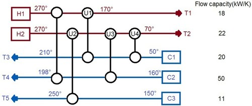
To demonstrate some of the issues that can arise with the gramian-based measures, we examine a heat exchanger network (HEN), which is a modified version of the configuration designed using pinch technology in Case study 1 by Escobar and Trierweiler (2013), illustrated in Figure 1. The modifications, implemented to make the HEN interesting from a control configuration selection perspective, amount to removing heaters and coolers and instead adding one more heat exchanger (HE) connected to a new stream (C3). The specifications for streams H1–H2 and C1–C2 are the same as in Escobar and Trierweiler (2013), and the new stream C3 has a flow capacity of 11 kW/K. The goal is to control the output temperatures T1 to T4 using bypasses over the heat exchangers U1–U4 to increase or decrease the energy transferred between the streams by the heat exchangers. T5 is assumed to be controlled further downstream and is thus not necessary to control here.

Figure 1. The studied heat exchanger network, where 5 heat exchangers transfer energy from the hot streams H1 and H2 to the cold streams T1, T2 and T3.

5.1. Heat exchanger models

The heat exchangers are modelled as a series of mixing tanks (15 mixing tanks were used to model U4, while 10 were found to be sufficient for the other HEs), as described by the multi-cell model by Mathisen et al. (1991). Moreover, the heat transfer coefficients have been modified from those in Escobar and Trierweiler (2013) to compensate for not using the logarithmic temperature differences, as discussed by Mathisen et al. (1994). All heat exchangers are modelled to have a residence time of 10 s. Pipe residence time and heat losses are not included in the model.

The actuators are controlled bypasses on the hot side of heat exchangers U1–U4. The HEs areas were therefore increased to retain the same steady-state temperatures when they bypass 10 of the stream, which consequently defines their stationary operating points. The complete system model was implemented in Matlab/Simulink and linearised with the bypass flow ratio on U1–U4 as inputs and the temperatures T1 to T4 as outputs. The Simulink model of the system is available at (https://github.com/fredbenchalmers/HEN–IO-pairing.).

5.2. The pairing problem

On the linearised model, different input output pairing algorithms were applied. The three previously mentioned gramian-based methods were used to derive decentralised control schemes. For comparison purposes, we used the classical RGA (Bristol, 1966) and the more recent ILQIA (Halvarsson, 2010) to derive non-gramian IM-based control schemes. The recommended pairing for each method is shown in Table 1, where we note that all the gramian based methods suggest the same pairing, different from the ILQIA and the RGA. To compare the suggested pairings decentralised PI control schemes were implemented and tuned using the lambda method applied on the open loop subsystems. Each of the control configurations was simulated on the nonlinear system both with reference steps on the output temperature of streams H1, H2, C1 and C2 and with disturbances on the input temperature and flow rate of streams H1, H2, C1 and C2. The size of the reference steps were two degrees and the size of the disturbances on the influent temperatures were negative two degrees. For flow rate, the system was tested with a decrease of 5% on the flow rate of H1 and H2, and with an increase of the flow rate of 5% on C1 and C2. These disturbances were chosen to be of a magnitude and direction that is possible for the system to completely compensate for. The simulations ran for 1000 s after the reference or disturbance step to fully observe its impact. For assessment, the mean quadratic deviation from the reference was devised as a cost, i.e. (3) $c={\int }_0^S(R(t)-Y(t){)}^T(R(t)-Y(t))\mathrm{d}t$(3) with $R(t)$ and $Y(t)$ being vectors containing the references and outputs, respectively, and S being the simulation time (in this case 1000 s). This was repeated for controllers designed with different values of η, and the result of those simulations are presented in Table 2.

Table 1. The results for the pairing suggestions for the HEN

	RGA	PM	HIIA	${\mathrm{\Sigma }}_2$	ILQIA
T1	U3	U1	U1	U1	U1
T2	U4	U4	U4	U4	U4
T3	U1	U2	U2	U2	U3
T4	U2	U3	U3	U3	U2

Table 2. Costs as defined by (3(3) $c={\int }_0^S(R(t)-Y(t){)}^T(R(t)-Y(t))\mathrm{d}t$(3) ) for different controller tuning η.

η	RGA	Gramian-based methods	ILQIA
1	235,065	342,149	263,431
2	136,606	210,002	204,696
3	95,950	126,502	156,832
3, 5	61,002	83,096	120,940
4	28,570	63,220	101,968
4, 5	16,528	41,376	85,213
5	7595	16,443	69,522
5, 5	1788	4771	53,765
6	1966	3533	35,830
6, 5	2154	3282	21,232
7	2344	3235	9054
7, 5	2537	3274	1570
8	2732	3358	990
10	3526	3897	1064
15	5568	5706	1687

A few conclusions can be drawn from these results. We can see that for aggressive control schemes, all controller schemes fail, resulting in an undamped oscillatory system. This is not unexpected as there are obvious limits on the actuators (they cannot bypass more than 100% of the stream or less than 0%), and therefore the controllers need to be somewhat cautious. If a reasonably tuned full multivariable MPC controller is used, the cost is approximatly 400. While this is considerably better then the lowest cost of 990, it is not sufficiently far away to indicate that a decentralised control is unreasonable for this system.

The control configuration suggested by the gramian based methods yields a considerably worse control for the best tuning than the ones recommended by the RGA or ILQIA, with a minimum cost of 3235 as opposed to 1788 or 990 (table entries in bold and blue). To examine why, we need to examine the IMs from the gramian-based methods: $\begin{array}{rl}PM& =\left[\begin{array}{cccc}0.15& 0.00046& 0.056& 0.13\\ 0& 0.000014& 0.0023& 0.55\\ 0.058& 0.00084& 0.00052& 0.017\\ 0& 0.0091& 0.026& 0\end{array}\right]\\ HIIA& =\left[\begin{array}{cccc}0.16& 0.0084& 0.097& 0.15\\ 0& 0.0015& 0.018& 0.29\\ 0.1& 0.011& 0.009& 0.054\\ 0& 0.032& 0.063& 0\end{array}\right]\\ {\mathrm{\Sigma }}_2& =\left[\begin{array}{cccc}0.17& 0.000035& 0.0054& 0.0038\\ 0& 0.0000039& 0.00081& 0.81\\ 0.0051& 0.00003& 0.0000072& 0.00022\\ 0& 0.00036& 0.00086& 0\end{array}\right].\end{array}$ As can be seen, all the values in the second columns are small compared to the largest values in the other columns. This means that when choosing elements from the matrix little importance is given to the second column. In other words, little importance is given to which element should be controlled by U2. The reason for this is that U2 is not particularly well suited for control compared to the other inputs, and therefore the values in its column are lower. However, one can still clearly see that the IMs suggest that U2 is much better suited for controlling T4 than controlling T3 but as can be seen in Table 1, none of the gramian-based measures recommend this pairing, while both non-gramian-based methods do. Similarly, we see that the third and fourth rows contain considerably less interaction than the other rows. Hence, less emphasis is placed on selecting a good actuator for T3 and T4 compared to T1 and T2.

It can be argued that this is a matter of scaling. However, all the inputs, being bypass percentages, are scaled from 0 to 1 as is the general convention to resolve the issue of input scaling for the gramian-based methods (Salgado & Conley, 2004). Moreover, all the outputs are tested with identically sized reference steps and can thus be said to be properly scaled as well. However, in this case, this scaling scheme appears to be insufficient. A method to alleviate this is to use the method presented in 2.3.1, that is to divide each element in the IM by the sum of all the elements in either its column or row. This ensures that either each input or each output is given equal weight. If we scale the PM, ${\mathrm{\Sigma }}_2$ and HIIA interaction measures with this method, we get the configurations shown in Table 3.

Table 3. The results for the optimal pairing of HEN using the new scaling.

	RGA	PM column scaling	HIIA column scaling	${\mathrm{\Sigma }}_2$ column scaling	PM row scaling	HIIA row scaling	${\mathrm{\Sigma }}_2$ row scaling	ILQIA
T1	U3	U3	U3	U1	U2	U2	U1	U1
T2	U4	U4	U4	U4	U4	U4	U4	U4
T3	U1	U1	U1	U3	U1	U1	U2	U3
T4	U2	U2	U2	U2	U3	U3	U3	U2

As can be seen in Table 3, with column scaling, we get the same control configurations as recommended by either the RGA or the ILQIA and consequently a lowered cost according to the assessment. With row scaling, we get a new configuration for the HIIA and PM. Testing with this configuration, however, yields a minimum cost of 3227, so this configuration is not significantly better than the unscaled gramian-based configuration.

To conclude, in this case, row scaling yields no noteworthy improvement, while column scaling yields a better configuration for all the tested gramian-based methods. Note that the method discussed in Section 2.3.2 would suggest that column scaling is preferable over row scaling for all the IMs.

5.3. Scaling using the Sinkhorn-Knopp algorithm

While we could observe here that in this case, normalising the IMs columns such that each input was given equal weight worked well, while normalising the rows such that each output was given equal weight yielded poorer results. There is another option to ensure that the IMs rows and columns all sum up to the same value, and hence all inputs and outputs are given equal weight. This can be achieved by iteratively alternating between scaling the elements by row sum and by column sum, which is the Sinkhorn-Knopp algorithm described in Section 2.3.3. Implementing the Sinkhorn-Knopp algorithm and stopping the algorithm when the error is less than ${10}^{-3}$ yields the control configurations presented in Table 4.

Table 4. Optimal pairing of the HEN using the Sinkhorn-Knopp algorithm.

	PM	HIIA	${\mathrm{\Sigma }}_2$
T1	U3	U3	U3
T2	U4	U4	U4
T3	U1	U1	U1
T4	U2	U2	U2

As can be seen, this resulted in the same configuration as the RGA, which while not being the configuration with the lowest cost, still yielded a considerably better result than the configuration recommended by the unscaled gramian-based measures. This is also the same configuration obtained with the PM and HIIA when applying column scaling. However, for the ${\mathrm{\Sigma }}_2$ method column scaling yielded a configuration with a lower cost.

6. Large-scale assessment of the methods

While the HEN example may have demonstrated potential benefits from rescaling the IMs, a single case study is insufficient to draw general conclusions. To quantitatively assess the methods, we have therefore used the MIMO model generator described by Bengtsson and Wik (2017) to generate a large number of linear MIMO-systems, with specifications shown in Table 5. The different scaling methods, i.e. by row sum, column sum, or both using the SK algorithm, were then applied to the generated models and the results were compared to using only the standard scaling. In addition, yet another approach was implemented. In this approach, one would either scale the rows or the columns, according to the reasoning in Section 2.3.2.

Table 5. Table showing the MIMO model generator (Bengtsson & Wik, 2017) settings.

Parameter	Value
Size
Number of inputs	5
Number of outputs	5
Minimum number of inputs affecting each output	4
Maximum number of inputs affecting each output	5
Minimum transfer function order	1
Maximum transfer function order	3
Minimum relative degree	1
Maximum relative degree	3
Dynamics
Maximum static gain	10–1000
Minimum pole time constant	1
Maximum pole time constant	10
Minimum damping for complex poles	0.1
Distinct time constants	false
Basing zeros time constants on poles when possible	true
Maximum overshoot percentage	10
Maximum undershoot percentage	25
Tolerance when determining overshoot/undershoot	0.01
Factor used to determine minimum time constant	100
Poles and Zeros
Maximum number of unstable poles	0
Minimum number of unstable poles	0
Maximum number of purely imaginary pole pairs	0
Minimum number of purely imaginary pole pairs	0
Percentage of unstable poles which are complex	0
Percentage of stable poles which are complex	20
Percentage of transfer functions with single integrators	0
Percentage of transfer functions with double integrators	0
Percentage of transfer functions with derivatives	0
Maximum number of non-minimum phase zeros	4
Minimum number of non-minimum phase zeros	0
Delay
Percentage of transfer functions with delay	10
Minimum delay	0
Maximum delay	0.5
Padé approximation order	2

For each control configuration, a decentralised control scheme was designed using both internal model control and the lambda method for varying values of η (the Matlab function tfest was used to approximate the transfer functions as the first-order systems which were then used for the lambda controller design). The entire feedback system was then tested both by reference step and by load disturbance. For the comparison, we define a cost using (3(3) $c={\int }_0^S(R(t)-Y(t){)}^T(R(t)-Y(t))\mathrm{d}t$(3) ) with a simulation time of 2000 time units after the reference step or the load disturbance. For each configuration, the cost was calculated for values of η ranging from 0.1 to 10 and the lowest cost was then saved. Having calculated this cost for each IM, each IM is given a score defined as $S=\frac{c_{min}}{c}$ where S is the score of the IM, c is the IMs cost, and $c_{min}$ is the lowest cost of all IMs for the system. The score was set to zero if the control scheme yielded unstable results. This measure was chosen to normalise the score of each iteration between 0 and 1 to ensure that the results on different systems are comparable.

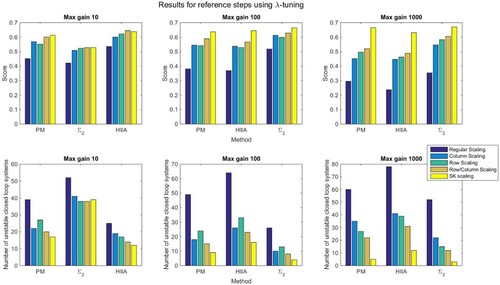
Three sets of 150 randomly generated systems were assessed having maximum static gains of 10, 100 and 1000 (minimum static gain was always 1). Both decentralised and sparse control schemes (for $\rho =3$) were implemented. For reference steps using λ-tuned controllers, the mean scores are presented in Figure 2. As taking the average scores may not always be the best metric, we also show how often the different methods yielded unstable results as a way to gauge how often the different methods failed completely. Further results for both λ-tuned controllers and IMC controllers, covering both reference steps and load disturbances, are presented in Tables 6 and 7 in Appendix.

Figure 2. Score and number of unstable results for reference steps using λ-tuning without feedforward on non-minimum phase systems.

The systems generated by the MIMO generator generally contained non-minimum phase transmission zeros. To evaluate how the presence of non-minimum phase dynamics affected the scaling methods, we also tested sets of systems without non-minimum phase transmission zeros (still with specifications according to Table 5). The result of this is included in Tables 8 and 9 in Appendix.

The large number of systems investigated allows a statistical evaluation whether the new scalings yield statistically significant improvements or not. Therefore, a t-test for paired samples was performed on the hypothesis that the scaled systems had a higher score than the unscaled system with a 95% confidence interval. This evaluation was carried out on both the systems with feed-forward and without. Similarly, statistical significance for number of unstable outcomes was determined by using a binomial sign test as described in Abdi (2007) evaluating if the scaling methods with a 0.95 probability reduced the number of unstable systems. The statistically significant improvements are highlighted in bold numbers in Tables 6–9.

As can be seen from the tables and Figure 2, the scaled IMs fare considerably better than the unscaled IMs. This improvement may be somewhat less pronounced when the gain variation in the TFM is small, which is in agreement with what was observed in the HE example, as high gain variation increases the likelihood that a row or column in the IM will have considerably less interaction than the other rows or columns. However, even in the case of low gain variation, there are statistically significant improvements for many of the scaling schemes.

One can also clearly see that the scaling method which yielded the best results was the one based on the Sinkhorn-Knopp algorithm, as it yielded the highest score and least number of unstable systems for most of the tested cases. The benefits of using the Sinkhorn-Knopp algorithm were the most apparent for high gain variation. With a high gain variation, one can see a very pronounced improvement for the PM and ${\mathrm{\Sigma }}_2$ method when using the Sinkhorn-Knopp algorithm compared to the other scaling methods. When using the HIIA, the improvement was somewhat smaller but still considerable.

The scaled systems also fared better both for decentralised and sparse control configurations. This indicates that the scaling methods can be used for both. However, the algorithm for implementing feedforward was somewhat cautious with $\rho =3$. Especially so for Sinkhorn-Knopp scaling, where there was often only a small difference between the cost for the sparse and the decentralised controllers. This also led to Sinkhorn-Knopp algorithm yielding comparably poor results in the cases where implementing feedforward had a very positive effect, namely, reference following for minimum phase systems. A more thorough feedforward implementation, tweaking ρ individually for the different scaling methods might have alleviated this issue.

It can also be noted that for all cases with high gain variation, SK scaling resulted in very few unstable outcomes, indicating that it is quite reliable for these types of systems. This clearly demonstrates the importance of rescaling the IMs in these cases, as with no additional scaling as many as one third or even one half of the closed loop systems were unstable.

Generally the results are similar regardless whether the controllers are tuned using IMC or the lambda method; in both cases, the Sinkhorn-Knopp algorithm generally outperformed the other scaling methods. We also experimented with using optimisation algorithms to find parameters for the PI controllers which minimised the cost and found that for the cases tested, the results were the same to those using IMC and λ-tuning.

As is shown in Figure 2, the results are similar regardless of whether one looks at mean cost or number of unstable outcomes.

Another observation is that without scaling it appears as if HIIA, on average, gave better results than PM and ${\mathrm{\Sigma }}_2$ for non-minimum phase systems, while the ${\mathrm{\Sigma }}_2$ method was superior for minimuim phase systems. However, SK-scaling has an effect on the performance in many cases exceeding the difference between the different methods.

Some caveats are however necessary. Only a few methods for automatic controller design was tested; it is possible that other control schemes might yield different results. Furthermore, other than changing the gain and the properties of the transmission zeros, only one set of model generator settings was used, modifications to other system properties may possibly also yield different results.

7. Conclusions and further work

The gramian-based interaction measures (IMs) are well known to be affected by scaling and the standard is therefore to scale all inputs and outputs to an equal range. A heat exchanger network control problem illustrated a case where the conventional scaling scheme failed. It was shown that by adapting the scaling of the IMs, this issue could be resolved. A few possible scaling methods were tested on a large number of systems using an MIMO model generator. It was found that all the tested scaling methods statistically improved the performance of the pairing methods consistently when designing a decentralised, as well as a sparse controller. The scaling method that yielded the best results was the one based on the Sinkhorn-Knopp algorithm, in particular, so when there are large variations in the static gains. In addition, this scaling method has the advantage of yielding results that are identical no matter what the original scaling of the inputs and outputs is.

There is, however, some room for further research in this field. The automatic implementation of sparse controllers is something that can be explored further, especially when using Sinkhorn-Knopp scaling.

Moreover, there are other possible control strategies and controller tuning on which the scaling methods can be explored. When testing the scaling methods here we specifically examined the impact of non-minimum phase transmission zeros and differences in static gain. There are of course other system properties which can be evaluated as well using the same techniques.

Disclosure statement

No potential conflict of interest was reported by the author(s).

Additional information

Funding

This work was supported by Preem AB and VINNOVA [2014-01945].

Appendix.

Tables with results

Table A1. Average score (S) and number of unstable outcomes (U) for the different methods with different gain variation for a reference step for non-minimum phase systems.

Maximum gain	10		100		1000		10		100		1000
Controller design method	Lambda						IMC
PM
Decentralised Control	S	U	S	U	S	U	S	U	S	U	S	U
No scaling	0.45	39	0.38	49	0.30	60	0.38	57	0.45	53	0.35	59
Column scaling	0.57	22	0.54	18	0.45	35	0.48	42	0.58	22	0.51	31
Row scaling	0.55	27	0.54	24	0.50	27	0.51	41	0.58	28	0.50	32
Row/column scaling	0.60	20	0.59	15	0.52	22	0.51	42	0.64	19	0.51	31
Sinkhorn-Knopp scaling	0.61	17	0.64	9	0.67	5	0.58	31	0.71	4	0.67	1
Sparse Control
No scaling.	0.46	36	0.39	52	0.31	60	0.38	59	0.43	57	0.40	63
Column scaling	0.59	23	0.61	26	0.58	39	0.46	48	0.57	34	0.58	39
Row scaling	0.56	28	0.52	32	0.47	35	0.47	48	0.50	39	0.48	38
Row/column scaling	0.62	20	0.62	21	0.60	27	0.50	44	0.63	27	0.58	34
Sinkhorn-Knopp scaling	0.61	17	0.64	9	0.67	5	0.58	31	0.71	4	0.67	1
${\mathbf{\Sigma }}_{\mathbf{2}}$
Decentralised Control
No scaling.	0.42	52	0.37	64	0.24	78	0.41	63	0.40	61	0.33	65
Column scaling	0.51	41	0.54	26	0.45	41	0.52	43	0.55	35	0.46	39
Row scaling	0.52	38	0.53	33	0.46	39	0.53	42	0.59	32	0.47	35
Row/column scaling	0.53	38	0.57	23	0.49	31	0.55	38	0.61	29	0.49	34
Sinkhorn-Knopp scaling	0.53	39	0.64	16	0.63	12	0.54	40	0.67	16	0.64	8
Sparse Control
No scaling.	0.44	52	0.37	66	0.25	76	0.40	64	0.40	64	0.33	63
Column scaling	0.53	40	0.61	28	0.52	46	0.51	46	0.57	43	0.51	44
Row scaling	0.50	42	0.51	38	0.47	40	0.52	46	0.53	44	0.41	46
Row/column scaling	0.54	39	0.61	26	0.52	36	0.56	40	0.60	35	0.49	43
Sinkhorn-Knopp scaling	0.53	39	0.64	16	0.63	12	0.54	40	0.67	16	0.65	8
HIIA
Decentralised Control
No scaling.	0.54	25	0.52	26	0.35	52	0.54	35	0.57	33	0.45	38
Column scaling	0.60	19	0.61	10	0.55	22	0.58	29	0.66	10	0.58	14
Row scaling	0.62	17	0.60	13	0.58	15	0.59	28	0.67	13	0.56	18
Row/column scaling	0.65	14	0.63	8	0.60	12	0.59	28	0.69	7	0.59	11
Sinkhorn-Knopp scaling	0.64	12	0.66	4	0.67	3	0.62	25	0.72	4	0.67	0
Sparse Control
No scaling.	0.53	25	0.54	29	0.37	56	0.54	36	0.56	36	0.45	50
Column scaling	0.60	19	0.61	14	0.64	26	0.58	29	0.67	14	0.67	23
Row scaling	0.62	17	0.59	16	0.56	26	0.59	29	0.62	21	0.54	30
Row/column scaling	0.65	14	0.63	11	0.65	17	0.59	28	0.70	10	0.67	17
Sinkhorn-Knopp scaling	0.64	12	0.66	4	0.67	3	0.62	25	0.72	4	0.68	0

Note: Bold values indicate statistically significant improvements compared to the system with no scaling.

Table A2. Average score (S) and number of unstable outcomes (U) for the different methods with different gain variation for a load disturbance for non-minimum phase systems.

Maximum gain	10		100		1000		10		100		1000
Controller design method	Lambda						IMC
PM
Decentralised Control	S	U	S	U	S	U	S	U	S	U	S	U
No scaling	0.46	39	0.42	50	0.36	61	0.35	61	0.51	52	0.46	59
Column scaling	0.58	23	0.61	18	0.56	36	0.45	45	0.65	21	0.64	30
Row scaling	0.56	29	0.62	24	0.57	28	0.49	42	0.64	26	0.65	32
Row/column scaling	0.61	21	0.66	15	0.61	23	0.49	43	0.70	18	0.65	30
Sinkhorn-Knopp scaling	0.61	19	0.71	10	0.78	6	0.56	32	0.80	3	0.82	1
Sparse Control
No scaling.	0.45	37	0.39	52	0.36	61	0.35	60	0.44	53	0.42	61
Column scaling	0.56	25	0.59	25	0.57	40	0.43	47	0.57	26	0.57	34
Row scaling	0.54	30	0.53	31	0.53	34	0.45	49	0.51	31	0.51	32
Row/column scaling	0.60	22	0.63	21	0.62	28	0.47	45	0.61	23	0.56	31
Sinkhorn-Knopp scaling	0.61	19	0.71	10	0.78	6	0.56	32	0.80	3	0.82	1
${\mathbf{\Sigma }}_{\mathbf{2}}$
Decentralised Control
No scaling.	0.45	52	0.42	66	0.29	79	0.44	58	0.48	61	0.45	65
Column scaling	0.54	41	0.64	28	0.53	43	0.52	43	0.64	34	0.64	38
Row scaling	0.56	39	0.61	34	0.55	40	0.56	41	0.68	32	0.62	35
Row/column scaling	0.56	39	0.67	25	0.57	33	0.57	38	0.70	28	0.67	33
Sinkhorn-Knopp scaling	0.57	40	0.75	17	0.75	13	0.57	39	0.78	15	0.85	7
Sparse Control
No scaling.	0.43	53	0.38	67	0.29	77	0.43	58	0.42	62	0.44	62
Column scaling	0.55	41	0.63	28	0.54	48	0.50	44	0.57	38	0.56	38
Row scaling	0.51	43	0.52	37	0.51	41	0.54	43	0.52	36	0.48	40
Row/column scaling	0.56	40	0.64	27	0.55	38	0.56	40	0.60	30	0.58	39
Sinkhorn-Knopp scaling	0.57	40	0.75	17	0.75	13	0.57	39	0.78	15	0.84	7
HIIA
Decentralised Control
No scaling.	0.55	25	0.57	27	0.43	53	0.52	37	0.62	33	0.58	38
Column scaling	0.61	20	0.67	11	0.65	23	0.56	31	0.74	10	0.74	14
Row scaling	0.63	18	0.67	13	0.67	16	0.58	29	0.75	13	0.72	18
Row/column scaling	0.65	15	0.70	9	0.71	13	0.57	30	0.78	7	0.76	11
Sinkhorn-Knopp scaling	0.65	13	0.74	5	0.79	4	0.60	26	0.81	3	0.81	0
Sparse Control
No scaling.	0.55	25	0.55	29	0.41	57	0.52	38	0.56	33	0.46	42
Column scaling	0.61	20	0.66	14	0.66	27	0.56	31	0.69	12	0.64	18
Row scaling	0.63	18	0.64	16	0.60	26	0.58	30	0.66	14	0.60	20
Row/column scaling	0.65	15	0.70	11	0.70	18	0.57	30	0.75	8	0.68	14
Sinkhorn-Knopp scaling	0.65	13	0.74	5	0.79	4	0.60	26	0.81	3	0.81	0

Note: Bold values indicate statistically significant improvements compared to the system with no scaling.

Table A3. Average score (S) and number of unstable outcomes (U) for the different methods with different gain variation for a reference step for minimum phase systems.

Maximum gain	10		100		1000		10		100		1000
Controller design method	Lambda						IMC
PM
Decentralised Control	S	U	S	U	S	U	S	U	S	U	S	U
No scaling	0.24	53	0.27	57	0.25	66	0.26	42	0.28	45	0.26	52
Column scaling	0.35	34	0.44	24	0.40	36	0.31	31	0.39	22	0.38	37
Row scaling	0.36	35	0.41	36	0.44	32	0.35	34	0.41	28	0.39	23
Row/column scaling	0.35	30	0.47	22	0.44	29	0.33	31	0.45	22	0.40	23
Sinkhorn-Knopp scaling	0.39	22	0.52	17	0.54	5	0.37	27	0.48	6	0.50	2
Sparse Control
No scaling.	0.26	54	0.27	58	0.27	57	0.27	50	0.34	43	0.27	55
Column scaling	0.35	36	0.51	29	0.56	29	0.31	36	0.50	28	0.47	41
Row scaling	0.36	37	0.44	36	0.50	31	0.35	38	0.44	34	0.41	30
Row/column scaling	0.34	33	0.52	26	0.54	26	0.34	32	0.54	24	0.46	27
Sinkhorn-Knopp scaling	0.39	22	0.52	17	0.54	5	0.37	27	0.48	6	0.50	2
${\mathbf{\Sigma }}_{\mathbf{2}}$
Decentralised Control
No scaling.	0.66	19	0.46	33	0.39	41	0.64	9	0.50	23	0.40	36
Column scaling	0.69	12	0.60	7	0.53	18	0.70	6	0.59	8	0.50	16
Row scaling	0.71	9	0.58	17	0.51	22	0.71	5	0.60	9	0.52	19
Row/column scaling	0.71	9	0.61	10	0.55	15	0.72	5	0.62	4	0.55	10
Sinkhorn-Knopp scaling	0.71	9	0.69	3	0.61	0	0.75	3	0.66	2	0.66	3
Sparse Control
No scaling.	0.70	16	0.50	33	0.43	39	0.70	11	0.55	22	0.43	34
Column scaling	0.74	9	0.73	8	0.69	16	0.73	13	0.76	10	0.69	19
Row scaling	0.77	9	0.66	17	0.59	18	0.77	5	0.66	15	0.54	22
Row/column scaling	0.74	8	0.73	7	0.69	12	0.76	8	0.76	7	0.63	14
Sinkhorn-Knopp scaling	0.71	9	0.69	3	0.61	0	0.75	3	0.66	2	0.66	3
HIIA
Decentralised Control
No scaling.	0.36	30	0.41	31	0.33	44	0.34	30	0.38	25	0.30	37
Column scaling	0.41	22	0.51	14	0.48	13	0.36	26	0.46	11	0.44	18
Row scaling	0.46	18	0.47	19	0.50	16	0.39	23	0.44	12	0.40	13
Row/column scaling	0.42	18	0.51	15	0.50	13	0.37	24	0.47	10	0.47	6
Sinkhorn-Knopp scaling	0.45	18	0.55	12	0.53	6	0.38	25	0.50	4	0.51	2
Sparse Control
No scaling.	0.36	30	0.43	33	0.39	46	0.34	30	0.41	28	0.35	45
Column scaling	0.41	22	0.54	15	0.65	15	0.36	26	0.51	11	0.55	22
Row scaling	0.46	18	0.48	20	0.57	15	0.39	23	0.45	12	0.44	27
Row/column scaling	0.42	18	0.52	17	0.62	14	0.37	24	0.49	10	0.55	11
Sinkhorn-Knopp scaling	0.45	18	0.55	12	0.53	6	0.38	25	0.50	4	0.51	2

Note: Bold values indicate statistically significant improvements compared to the system with no scaling.

Table A4. Average score (S) and number of unstable outcomes (U) for the different methods with different gain variation for a load disturbance for minimum phase systems.

Maximum gain	10		100		1000		10		100		1000
Controller design method	Lambda						IMC
PM
Decentralised Control	S	U	S	U	S	U	S	U	S	U	S	U
No scaling	0.22	53	0.32	57	0.36	66	0.29	43	0.39	44	0.35	53
Column scaling	0.35	34	0.52	24	0.62	36	0.32	32	0.53	24	0.53	36
Row scaling	0.34	35	0.47	36	0.61	32	0.37	34	0.55	26	0.54	24
Row/column scaling	0.35	30	0.55	22	0.63	29	0.34	31	0.60	23	0.57	24
Sinkhorn-Knopp scaling	0.38	22	0.58	17	0.77	5	0.38	27	0.63	8	0.73	3
Sparse Control
No scaling.	0.23	54	0.30	57	0.33	57	0.29	45	0.37	40	0.34	55
Column scaling	0.33	36	0.49	26	0.54	29	0.31	32	0.49	27	0.49	36
Row scaling	0.32	37	0.44	36	0.53	29	0.36	34	0.49	23	0.51	25
Row/column scaling	0.33	33	0.50	24	0.56	24	0.33	30	0.54	24	0.54	23
Sinkhorn-Knopp scaling	0.38	22	0.58	17	0.77	5	0.38	27	0.63	8	0.73	3
${\mathbf{\Sigma }}_{\mathbf{2}}$
Decentralised Control
No scaling.	0.72	19	0.56	33	0.55	41	0.79	7	0.69	24	0.58	35
Column scaling	0.77	12	0.76	7	0.78	18	0.82	6	0.82	9	0.75	15
Row scaling	0.77	9	0.72	17	0.72	22	0.83	5	0.78	10	0.75	19
Row/column scaling	0.78	9	0.76	10	0.79	15	0.84	5	0.82	5	0.81	10
Sinkhorn-Knopp scaling	0.78	9	0.86	3	0.89	0	0.83	3	0.86	2	0.92	2
Sparse Control
No scaling.	0.69	16	0.55	33	0.53	39	0.65	7	0.63	22	0.56	31
Column scaling	0.78	9	0.73	6	0.75	16	0.76	5	0.76	8	0.66	16
Row scaling	0.72	8	0.67	16	0.63	18	0.70	4	0.68	8	0.66	14
Row/column scaling	0.78	8	0.72	6	0.75	12	0.75	4	0.74	5	0.71	10
Sinkhorn-Knopp scaling	0.78	9	0.86	3	0.89	0	0.83	3	0.86	2	0.92	2
HIIA
Decentralised Control
No scaling.	0.34	30	0.48	31	0.48	44	0.35	31	0.49	26	0.42	38
Column scaling	0.40	22	0.60	14	0.73	13	0.38	25	0.60	12	0.63	17
Row scaling	0.44	18	0.56	19	0.70	16	0.41	23	0.61	12	0.58	14
Row/column scaling	0.41	18	0.59	15	0.72	13	0.38	23	0.62	10	0.68	7
Sinkhorn-Knopp scaling	0.45	18	0.62	12	0.77	6	0.40	24	0.65	6	0.75	3
Sparse Control
No scaling.	0.34	30	0.46	32	0.44	43	0.35	31	0.45	27	0.37	39
Column scaling	0.40	22	0.59	14	0.67	13	0.38	25	0.58	12	0.60	19
Row scaling	0.44	18	0.55	20	0.60	13	0.41	23	0.56	11	0.52	17
Row/column scaling	0.41	18	0.59	16	0.68	13	0.38	23	0.60	10	0.64	7
Sinkhorn-Knopp scaling	0.45	18	0.62	12	0.77	6	0.40	24	0.65	6	0.75	3

Note: Bold values indicate statistically significant improvements compared to the system with no scaling.

References

- Abdi, H. (2007). Binomial distribution: Binomial and sign tests. Encyclopedia of measurement and statistics (Vol. 1). SAGE publications.
- Ang, K. H., Chong, G., & Li, Y. (2005, July). PID control system analysis, design, and technology. IEEE Transactions on Control Systems Technology, 13(4), 559–576. https://doi.org/https://doi.org/10.1109/TCST.2005.847331
- Arranz, M. C., & Birk, W. (2009). New methods for structural and functional analysis of complex processes. Control applications, (CCA) & intelligent control, (ISIC) (pp. 487–494). IEEE.
- Bengtsson, F., & Wik, T. (2017). A multiple input, multiple output model generator (Tech. Rep.). Department of Signals and Systems, Chalmers University of Technology. https://research.chalmers.se/publication/253490
- Birk, W., & Medvedev, A. (2003). A note on gramian-based interaction measures. Proceedings of european control conference (ECC) (pp. 2625–2630). IEEE.
- Bristol, E. (1966). On a new measure of interaction for multivariable process control. IEEE Transactions on Automatic Control, 11, 133–134. https://doi.org/https://doi.org/10.1109/TAC.1966.1098266
- Conley, A., & Salgado, M. E. (2000). Gramian based interaction measure. Proceedings of the 39th IEEE conference on decision and control (Vol. 5, pp. 5020–5022). IEEE.
- Escobar, M., & Trierweiler, J. O. (2013). Optimal heat exchanger network synthesis: A case study comparison. Applied Thermal Engineering, 51(1–2), 801–826. https://doi.org/https://doi.org/10.1016/j.applthermaleng.2012.10.022
- Fatehi, A. (2011). Automatic pairing of large scale MIMO plants using normalised RGA. International Journal of Modelling, Identification and Control, 14(1–2), 37–45. https://doi.org/https://doi.org/10.1504/IJMIC.2011.042338
- Grosdidier, P., Morari, M., & Holt, B. R. (1985). Closed-loop properties from steady-state gain information. Industrial & Engineering Chemistry Fundamentals, 24(2), 221–235. https://doi.org/https://doi.org/10.1021/i100018a015
- Halvarsson, B. (2010). Interaction analysis in multivariable control systems: Applications to bioreactors for nitrogen removal [Doctoral dissertation, Uppsala University, Division of Systems and Control, Automatic control]. http://uu.diva-portal.org/smash/get/diva2:309623/FULLTEXT01.pdf
- Knight, P. A. (2008). The Sinkhorn–Knopp algorithm: Convergence and applications. SIAM Journal on Matrix Analysis and Applications, 30(1), 261–275. https://doi.org/https://doi.org/10.1137/060659624
- Mathisen, K. W., Morari, M., & Skogestad, S. (1994). Dynamic models for heat exchangers and heat exchanger networks. Computers & Chemical Engineering, 18, S459–S463. https://doi.org/https://doi.org/10.1016/0098-1354(94)80075-8
- Mathisen, K. W., Skogestad, S., & Wolff, E. A. (1991). Controllability of heat exchanger networks (Vol. 152). AIChE Annual Meeting, LA, USA.
- Panagopoulos, H., Hägglund, T., & Åström, K. J. (1997). The lambda method for tuning PI controllers (Vol. 280, Tech. Rep. No. 7564). Department of Automatic Control, Lund Institute of Technology.
- Rivera, D. E., Morari, M., & Skogestad, S. (1986). Internal model control: PID controller design. Industrial & Engineering Chemistry Process Design and Development, 25(1), 252–265. https://doi.org/https://doi.org/10.1021/i200032a041
- Salgado, M. E., & Conley, A. (2004). MIMO interaction measure and controller structure selection. International Journal of Control, 77(4), 367–383. https://doi.org/https://doi.org/10.1080/0020717042000197631
- Sinkhorn, R., & Knopp, P. (1967). Concerning nonnegative matrices and doubly stochastic matrices. Pacific Journal of Mathematics, 21(2), 343–348. https://doi.org/https://doi.org/10.2140/pjm doi: https://doi.org/10.2140/pjm.1967.21.343
- van de Wal, M., & de Jager, B. (2001). A review of methods for input/output selection. Automatica, 37(4), 487–510. https://doi.org/https://doi.org/10.1016/S0005-1098(00)00181-3
- Wittenmark, B., & Salgado, M. E. (2002). Hankel-norm based interaction measure for input-output pairing. Proceedings of the 2002 IFAC World congress (Vol. 139). Elsevier.
- Zhu, Z. X. (1996). Variable pairing selection based on individual and overall interaction measures. Industrial & Engineering Chemistry Research, 35(11), 4091–4099. https://doi.org/https://doi.org/10.1021/ie960143n