Input-to-state stability for system identification with continuous-time Runge–Kutta neural networks

Abstract

Runge–Kutta neural networks (RKNN) bridge the gap between continuous-time advantages and the discrete-time nature of any digital controller. RKNN defines a neural network in a continuous-time setting and explicitly discretises it by a variable sample time Runge–Kutta method. As a result, a-priori model knowledge such as the well-known continuous-time state space model can easily be incorporated directly into the neural network weights. Additionally, RKNN preserves a long-term prediction accuracy and a reduced parameter precision requirement.

In this contribution, we enhance RKNN with global-asymptotic stability (GAS) and input-to-state stability (ISS) criteria. Based on a Lyapunov function, we develop constraints on the neural network weights for an arbitrary sample time. The constraints are independent of any measurements, have only a few hyperparameters, can be combined with any standard constraint optimisation algorithm and guarantee stability already during training. We apply the algorithm on two public real-world nonlinear identification tasks, an electro-mechanical positioning system and a cascaded water tank benchmark. Both benchmarks are solved with the same hyperparameters and the presented method is competitive to nonlinear identification methods beyond neural networks in the literature. In prediction configuration, all other black-box nonlinear identification approaches are outperformed regarding root mean squared error (RMSE) by an order of magnitude on the cascaded tank benchmark.

Keywords:

• Runge–Kutta neural networks
• input-to-state stability
• continuous-time neural networks
• discrete-time neural networks
• state space models
• nonlinear identification

1. Introduction

Nonlinear system identification is a core discipline in control engineering (e.g. Nelles, 2001; Sjoberg et al., 1995). For more than 30 years, neural networks are developed and widely applied for the identification of nonlinear dynamic systems (e.g. Ahmed et al., 2010; Chen et al., 1990; Deflorian et al., 2010; Haykin, 1990; Narendra & Parthasarathy, 1990; Weigand et al., 2020; Williams & Zipser, 1989). Many contributions focus on discrete-time neural networks. As pointed out by Y. J. Wang and Lin (1998), there are several problems in using discrete-time neural networks: larger approximation errors are induced by the assumed first-order discretisation, the long-term prediction accuracy is usually upgradable and the neural network can only predict the system behaviour at fixed time intervals. A variable sample time¹ in training and application leads to complete model failure. This is mainly because feed forward networks and recurrent neural networks tend to learn the system states instead of the change rates of system states. Thereby the discrete sample time is inseparably connected to the neural network weights.

Another approach are continuous-time neural networks. This type of networks do not suffer from the aforementioned disadvantages. However, continuous-time neural networks do not consider the discrete-time nature of measurements or any digital controller. They often require a quasi-continuous sample time. This results in a large amount of training data and a restriction of applications. In industrial real-time applications, a high sample time can be prohibitive and thus the discrete-time nature of the measurements has to be taken into account. Runge–Kutta neural networks (RKNN) bridge this gap by constructing a neural network in continuous-time domain and integrating the Runge–Kutta (RK) approximation method explicitly. Thus a precise estimate of the change rates of the system states is possible (Y. J. Wang & Lin, 1998). Therefore, RKNN do not suffer from the aforementioned disadvantages of discrete-time or continuous-time neural networks and are superior in generalisation and long-term prediction accuracy, as theoretically proven by Y. J. Wang and Lin (1998) and shown in simulations by Efe and Kaynak (2000). More recently, Forgione and Piga (2021a) and Mavkov et al. (2020) achieved very good results with continuous-time neural networks for system identification.

In general, model stability is a key consideration for nonlinear system identification especially with data-based neural networks. Accordingly, the stability properties of discrete-time neural networks are widely studied (e.g. Barabanov & Prokhorov, 2002; Hu & Wang, 2002b; L. Wang & Xu, 2006; Yu, 2004). The continuous-time model stability properties are broadly analysed too, see, e.g. Hu and Wang (2002a) for stability and Sanchez and Perez (1999) for the more general concept of input-to-state stability (ISS). ISS extends the stability criterion of global asymptotic stability (GAS) in the sense of Lyapunov to non-autonomous systems, i.e. systems with an input unequal to zero. Sontag (2008) shows that some GAS stable systems can diverge even for some inputs that converge to zero.

However, due to the explicit transfer to the discrete-time domain, neither the discrete-time nor the continuous-time stability criteria are applicable for RKNN. Only a sample time-dependent criterion can guarantee ISS for RKNN. Therefore, we derive sample time-dependent ISS constraints on the neural network weights in this contribution. The ISS constraints ensure that all predicted states remain bounded. This holds always true, including but not limited to all inputs, to long-term predictions and to feedback loops containing the neural network in a model based controller with potentially noisy state measurements. Note that the presented algorithm enforces model stability even if the underlying process is unstable. In this case, the algorithm generates model errors, identifying a stable model for an unstable process.

The contributions of this paper can be summarised as follows:

• A discussion of bridging the gap between continuous-time models and the discrete-time nature of digital controllers with RKNN.

• Sample time-dependent ISS and GAS stability guarantees for RKNN.

• A comparison of RKNN with methods beyond neural networks for system identification on two public, real-world benchmarks. The benchmarks are an electro-mechanical positioning system and a cascaded water tank system. To the best of our knowledge and in prediction configurations, the presented approach outperforms all other methods applied on the same benchmarks.

The remainder of this paper is organised as follows. In Section 2, we illustrate the contributions regarding stability with two simple examples. In Section 3, the RKNN is defined and in Section 4 the properties of continuous-time neural networks are discussed. In Section 5, some preliminaries regarding stability and in Section 6, the stability constraints for the RKNN are presented. We apply the algorithm to two real-world identification tasks in Section 7 and make concluding remarks in Section 8.

2. Illustrative examples

The core contribution regarding stability can be illustrated using two simple examples, accounting for the continuous-time stability and the discretisation method, as both aspects contribute to ISS. First, consider a learned continuous-time neural network which is clearly GAS, but its states tend to infinity in the presence of bounded inputs. This example underlines the importance of ISS instead of GAS.

Consider a continuous-time neural network with one state $x\left(t\right)\in \mathbb{R}$, one input $u\left(t\right)\in \mathbb{R}$, continuous-time $t\in \mathbb{R}$, hyperbolic tangent activation function $\tanh (\cdot )$, no bias weights and two neurons in the hidden layer, (1) $\begin{array}{r}\dot{x}\left(t\right)=\left[\begin{array}{cc}-1& 10\end{array}\right]\tanh \left(\left[\begin{array}{c}1\\ 0\end{array}\right]x\left(t\right)+\left[\begin{array}{c}0\\ 1\end{array}\right]u\left(t\right)\right).\end{array}$(1) The network (1(1) $\begin{array}{r}\dot{x}\left(t\right)=\left[\begin{array}{cc}-1& 10\end{array}\right]\tanh \left(\left[\begin{array}{c}1\\ 0\end{array}\right]x\left(t\right)+\left[\begin{array}{c}0\\ 1\end{array}\right]u\left(t\right)\right).\end{array}$(1) ) is clearly GAS as the autonomous system reduces to $\dot{x}\left(t\right)=-\tanh \left(x\right)$ and converges to zero. But for any given input $u\left(t\right)\ge 2$ (and including any upper bound, e.g. $u\left(t\right)\le {10}^6$), we get $\begin{array}{rl}\dot{x}\left(t\right)& =-\tanh \left(x\right(t\left)\right)+10\tanh \left(u\right(t\left)\right)\\ & >-\tanh \left(x\right(t\left)\right)+9>8\end{array}$ and the system trajectory tends to infinity although the input is bounded. The following second example shows that even an ISS neural network can become unstable if neural network constrains do not account for the sample time $h\in \mathbb{R}$. Consider a standard state space neural network with eigenfrequency ${\omega }_0=10\frac{1}{s}$, damping D = 0.5 and input gain K = 1. The network consists of two states, one input, no bias terms and no hidden layers, (2) $\begin{array}{r}\dot{x}\left(t\right)=\left[\begin{array}{cc}0& 1\\ -{\omega }_0^2& -D{\omega }_0\end{array}\right]x\left(t\right)+\left[\begin{array}{c}0\\ K{\omega }_0^2\end{array}\right]u\left(t\right)\end{array}$(2) and is GAS and ISS in the continuous domain (as it is input-affine and the real parts of all eigenvalues are negative). 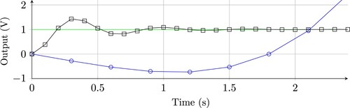Assume (2(2) $\begin{array}{r}\dot{x}\left(t\right)=\left[\begin{array}{cc}0& 1\\ -{\omega }_0^2& -D{\omega }_0\end{array}\right]x\left(t\right)+\left[\begin{array}{c}0\\ K{\omega }_0^2\end{array}\right]u\left(t\right)\end{array}$(2) ) is time discretised by a fourth-order Runge–Kutta method and a sample frequency much greater than the eigenfrequencies. 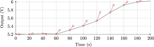As shown exemplary in Figure 1 for a step response, the discrete-time trajectory for (2(2) $\begin{array}{r}\dot{x}\left(t\right)=\left[\begin{array}{cc}0& 1\\ -{\omega }_0^2& -D{\omega }_0\end{array}\right]x\left(t\right)+\left[\begin{array}{c}0\\ K{\omega }_0^2\end{array}\right]u\left(t\right)\end{array}$(2) ) tends to infinity for h = 0.3s although it is stable for h = 0.1s. This trade off between neural network weights and sample time in general is non-trivial. To the best of our knowledge, the presented stability constraints are the only ones that can enforce ISS in the given examples.

Figure 1. Step response of a stable and unstable time discretisation of (2(2) $\begin{array}{r}\dot{x}\left(t\right)=\left[\begin{array}{cc}0& 1\\ -{\omega }_0^2& -D{\omega }_0\end{array}\right]x\left(t\right)+\left[\begin{array}{c}0\\ K{\omega }_0^2\end{array}\right]u\left(t\right)\end{array}$(2) ). Circles and squares represent each discrete-time step. Green: Step input. Black: Stable discretisation. Blue: unstable discretisation.

3. Runge–Kutta neural networks

The RKNN consists of a continuous-time neural network embedded in an explicit S-stage RK method. The neural network is defined by the differential equations (3a) $\begin{array}{rl}\dot{\hat{x}}& =f_{\mathrm{N}\mathrm{N}}(\hat{x},\tilde{u})=W_x^l\hat{x}+W_u^l\tilde{u}\\ & +W_a^o\sigma \left(W_x^h\hat{x}+W_u^h\tilde{u}\right),\end{array}$(3a) (3b) $\begin{array}{rl}\hat{y}& =h_{\mathrm{N}\mathrm{N}}(\hat{x},\tilde{u})=W_x^{H,l}\hat{x}+W_u^{H,l}\tilde{u}\\ & +W_a^{H,o}\sigma \left(W_x^{H,h}\hat{x}+W_u^{H,h}\tilde{u}\right)\end{array}$(3b) where the state network is $f_{\mathrm{N}\mathrm{N}}(\hat{x},\tilde{u}):{\mathcal{R}}^{N_X}\times l_{\mathrm{\infty }}^{N_U+1}\to {\mathbb{R}}^{N_X}$ with sequence space $l_{\mathrm{\infty }}^{N_U+1}$, 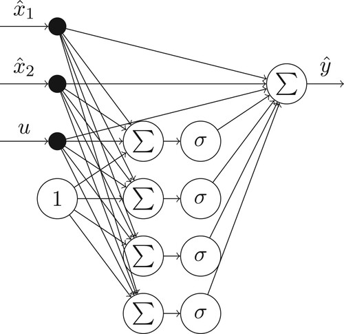the output network is $h_{\mathrm{N}\mathrm{N}}(\hat{x},\tilde{u}):{\mathbb{R}}^{N_X}\times l_{\mathrm{\infty }}^{N_U+1}\to {\mathbb{R}}^{N_Y}$, the augmented input is $\tilde{u}\in l_{\mathrm{\infty }}^{N_U+1}$, the true and calculated outputs are $y\in {\mathbb{R}}^{N_Y}$ and $\hat{y}\in {\mathbb{R}}^{N_Y}$ respectively, the true and calculated states are $x\in {\mathbb{R}}^{N_X}$ and $\hat{x}\in {\mathbb{R}}^{N_X}$ respectively. The nomenclature of the weight matrices W is as follows: superscripts l, o and h denote the linear matrix, output matrix and hidden layer matrix for the state network. Superscript H corresponds to the respective layers of the output network $h_{\mathrm{N}\mathrm{N}}(\hat{x},\tilde{u})$. Subscripts x, u and a refer to state weights, augmented input weights and activation function weights respectively. Note that the augmented input is bounded, i.e. there is an upper bound $M\in \mathbb{R}$ so that $\parallel \tilde{u}\left(t\right){\parallel }_{\mathrm{\infty }}<M$ holds for all times t. The augmented input $\tilde{u}$ is composed of the input $u\in l_{\mathrm{\infty }}^{N_U}$ and a constant for taking bias terms into account $\tilde{u}=[u^T,1{]}^T.$ Several neural networks can be applied, as long as the activation function $\sigma (\cdot )$ of the state network is Lipschitz continuous and $0\le \frac{\sigma \left(v_i\right)}{v_i}\le 1$ for any argument $v_i\in {\mathbb{R}}_{\ne 0}^{}$ holds. The activation function $\sigma (\cdot )$ is defined element-wise. There are no requirements for the activation function of the output network ${\sigma }^H(\cdot )$. In this work, we present and compare two types of activation functions, hyperbolic tangent (TANH) and rectified linear units (ReLU). In the case of TANH, the activation function is $\sigma :v\mapsto [\tanh (v_1),\dots ,\tanh (v_{N_N}){]}^T$ and in the ReLU case, the activation function is $\sigma :v\mapsto [max(v_1,0),\dots ,max(v_{N_N},0){]}^T$ with the number of hidden units $N_N$. The state and output network are depicted in Figures 2 and 3.

Figure 2. State network $f_{{}_{\mathrm{N}\mathrm{N}}}(\hat{x},\tilde{u})$.

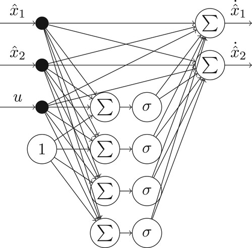
Figure 3. Output network $h_{{}_{\mathrm{N}\mathrm{N}}}(\hat{x},\tilde{u})$.

The continuous-time neural network (3a(3a) $\begin{array}{rl}\dot{\hat{x}}& =f_{\mathrm{N}\mathrm{N}}(\hat{x},\tilde{u})=W_x^l\hat{x}+W_u^l\tilde{u}\\ & +W_a^o\sigma \left(W_x^h\hat{x}+W_u^h\tilde{u}\right),\end{array}$(3a) ) is embedded in an S-stage explicit RK method with sample time h such that the discrete-time system (4a) $\begin{array}{rl}{\hat{x}}_{n+1}& =F_{{}_{\mathrm{R}\mathrm{K}\mathrm{N}\mathrm{N}}}({\hat{x}}_n,{\tilde{u}}_n),\end{array}$(4a) (4b) $\begin{array}{rl}{\hat{y}}_n& =H_{{}_{\mathrm{R}\mathrm{K}\mathrm{N}\mathrm{N}}}({\hat{x}}_n,{\tilde{u}}_n)\end{array}$(4b) is generated. We define the discrete sample time $n\in \mathbb{N}$ so that ${\hat{x}}_n=\hat{x}(t=nh)$. The RK scheme provides the rule to compute (4a(4a) $\begin{array}{rl}{\hat{x}}_{n+1}& =F_{{}_{\mathrm{R}\mathrm{K}\mathrm{N}\mathrm{N}}}({\hat{x}}_n,{\tilde{u}}_n),\end{array}$(4a) ) from (3a(3a) $\begin{array}{rl}\dot{\hat{x}}& =f_{\mathrm{N}\mathrm{N}}(\hat{x},\tilde{u})=W_x^l\hat{x}+W_u^l\tilde{u}\\ & +W_a^o\sigma \left(W_x^h\hat{x}+W_u^h\tilde{u}\right),\end{array}$(3a) ) for a given sample time h. The general S-stage RK method is defined by the discrete-time system (5a) $\begin{array}{rl}{\hat{x}}_{n+1}& ={\hat{x}}_n+h\sum _{s=1}^S{b}_{B,s}{g}_{n,s},\end{array}$(5a) (5b) $\begin{array}{rl}{g}_{n,s}& =f\left({\hat{x}}_n+h\sum _{j=1}^S{a}_{B,s,j}{g}_{n,j},u(nh+c_{B,s}h)\right)\end{array}$(5b) with the butcher coefficients $a_{B,s,j},b_{B,s},c_{B,s}$ and $\sum _{s=1}^S{b}_{B,s}=1,c_{B,s}=\sum _{j=1}^S{a}_{B,s,j}$ (see Butcher, 2016). The coefficients of the RK method are usually collected in vectors and a matrix and are represented by the Butcherarray $c_B{A}_B{b}_B^T.$

The RK scheme (5a(5a) $\begin{array}{rl}{\hat{x}}_{n+1}& ={\hat{x}}_n+h\sum _{s=1}^S{b}_{B,s}{g}_{n,s},\end{array}$(5a) ) is completely determined by the parameter matrix and vectors $A_B,b_B$ and $c_B$. Note that for an explicit RK method, the matrix $A_B$ is lower triangular (see Butcher, 2016). Although the notation (5a(5a) $\begin{array}{rl}{\hat{x}}_{n+1}& ={\hat{x}}_n+h\sum _{s=1}^S{b}_{B,s}{g}_{n,s},\end{array}$(5a) ) allows a varying $\tilde{u}$ within the sample interval, we assume it to be constant during one arbitrarily short sample interval. In the following, we focus on the state network and set $g_{n,s}=f_{{}_{\mathrm{N}\mathrm{N}}}\left({\hat{x}}_n+h\sum _{j=1}^S{a}_{B,s,j}{g}_{n,j},\tilde{u}\left(nh\right)\right).$

The solution of the output network is straightforward and does not affect any stability considerations since it does not contain any derivatives or any feedback, ${\hat{y}}_n=H_{{}_{\mathrm{R}\mathrm{K}\mathrm{N}\mathrm{N}}}({\hat{x}}_n,{\tilde{u}}_n)=h_{{}_{\mathrm{N}\mathrm{N}}}({\hat{x}}_n,{\tilde{u}}_n).$ The classical 4-stage RK method as neural network graph is depicted in Figure 4, with the state network $f_{{}_{\mathrm{N}\mathrm{N}}}(\hat{x},\tilde{u})$ and output network $h_{{}_{\mathrm{N}\mathrm{N}}}(\hat{x},\tilde{u})$ as presented in Figures 2 and 3 respectively.

Figure 4. Representation of the classical RKNN architecture. The RKNN explicitly includes the integration method as a neural network graph extension. A similar figure is presented in Uçak (2020).

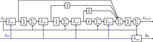
Equivalent to Figure 4, the classical 4-stage RK method is given by the equations (2) $\begin{array}{rl}{g}_{n,1}& =f_{{}_{\mathrm{N}\mathrm{N}}}\left({\hat{x}}_n,{\tilde{u}}_n\right),\end{array}$(2)   $\begin{array}{rl}{g}_{n,2}& =f_{{}_{\mathrm{N}\mathrm{N}}}\left({\hat{x}}_n+\frac{h}{2}{g}_{n,1},{\tilde{u}}_n\right),\end{array}$    $\begin{array}{rl}{g}_{n,3}& =f_{{}_{\mathrm{N}\mathrm{N}}}\left({\hat{x}}_n+\frac{h}{2}{g}_{n,2},{\tilde{u}}_n\right),\end{array}$    $\begin{array}{rl}{g}_{n,4}& =f_{{}_{\mathrm{N}\mathrm{N}}}\left({\hat{x}}_n+h{g}_{n,3},{\tilde{u}}_n\right),\end{array}$    $\begin{array}{rl}{\hat{x}}_{n+1}& ={\hat{x}}_n+\frac{h}{6}\left(g_{n,1}+2g_{n,2}+2g_{n,3}+g_{n,4}\right),\end{array}$    $\begin{array}{rl}{\hat{y}}_n& =h_{{}_{\mathrm{N}\mathrm{N}}}\left({\hat{x}}_n,{\tilde{u}}_n\right).\end{array}$ 

4. Properties of continuous-time neural networks

Depending on the application, the presented model is capable of two configurations. In a (one-step-ahead) prediction configuration (e.g. Y. J. Wang & Lin, 1998), the state x is completely measured for all time steps. Each predicted output and state, ${\hat{y}}_{n+1}$ and ${\hat{x}}_{n+1}$, is estimated based on the previously measured state and input, i.e. $x_n$ and ${\tilde{u}}_n$. The estimated state ${\hat{x}}_n$ is not fed back into the state network. As a consequence, a one-step prediction mode leads to a fast training and enables parallel computation. However, training in one-step prediction reduces accuracy for long-term predictions if the model is not even unstable (without the presented constraints).

If long-term estimation is required in the application, it cannot be neglected in the training. Therefore, in a (multi-step-ahead) simulation configuration (e.g. Deflorian, 2010), only the initial state measurement $x_0$ is required and all proceeding states are recursively taken from previous calculations. So, each successive simulated state ${\hat{x}}_{n+1}$ in the training depends on the previous state estimate ${\hat{x}}_n$ and on the input ${\tilde{u}}_n$. The feedback of estimated states leads to a potential accumulation of state errors and is therefore more comprehensive. The difference regarding estimation performance between simulation and prediction configuration is 2 orders of magnitude for both presented benchmarks (see Section 7).

However, defining neural networks in continuous-time and discretising by RK methods leads to several advantages:

1. Continuous-time neural networks have a great analogy to the well-known state–space model, making it easy to incorporate a-priori knowledge. For example, $\begin{array}{rl}\dot{x}\left(t\right)& =A_{S}x\left(t\right)+B_{S}u\left(t\right),\\ y\left(t\right)& =C_{S}x\left(t\right)+D_{S}u\left(t\right)\end{array}$ is equivalent to $\begin{array}{rlrlrl}{W}_x^l& =A_S,& W_u^l& =\left[B_S,0\right],& & \\ W_x^{H,l}& =C_S,& W_u^{H,l}& =\left[D_S,0\right],& & \\ W_a^o& =0,& W_x^h& =0,& W_u^h& =0,\\ W_a^{H,o}& =0,& W_x^{H,h}& =0,& W_u^{H,h}& =0.\end{array}$ So the linear weight matrices $W_x^l,W_u^l,W_x^{H,l}$ and $W_u^{H,l}$ are capable of modelling a linear core model while the matrices $W_a^o,W_x^h,W_u^h,W_a^{H,o},W_x^{H,h}$ and $W_u^{H,h}$ can focus on nonlinear effects.

2. Discretising by explicit RK methods enables a simple integration of variable sample times. The sample times in training can differ from the sample time in the application by adjusting h. This enables a reduction of the data set in training and therefore reducing computational effort. In this case, the presented stability constraints have to apply the maximum sample time. In neural networks in a discrete-time setting varying sample time is very difficult, because the sample time is directly intertwined with the weights (e.g. Hu & Wang, 2002b). However, discrete-time networks are a special case of the presented algorithm. If a simple discretisation by Euler and a sample time of h = 1 is selected, we obtain ${\hat{x}}_{n+1}=W_x^l{\hat{x}}_n+W_u^l{\tilde{u}}_n+W_a^o\sigma (W_x^h{\hat{x}}_n+W_u^h{\tilde{u}}_n).$ Covering this as a special case, the presented stability constraints in our contribution enhance the work of Hu and Wang (2002b) and enable full continuous-time advantages in a discrete-time formulation.

3. Defining a model in continuous-time reduces the necessary parameter precision for a good approximation. For instance, consider the PT2 transfer function $G\left(s\right)=\frac{100}{s^2+14s+100}.$ Selecting a sample time of 1 ms the MATLAB command $c2d$ calculates the corresponding z-transfer function $G\left(z\right)=\frac{0.497670667119z+0.495353610317}{z^2-1.985998241835z+0.986097544263}.$ For the same model, the number of significant parameter digits increases from 3 digits to 12. In theory, considering an Euler discretisation, a small sample time always leads to an increase of significant parameter digits. The more precision is required in the model parameters, usually the more complicated the optimisation problem becomes. In discrete-time models, even small deviations of parameters accumulate over time to notable errors. Furthermore, discrete-time model stability tends to be more sensitive to parameter errors than continuous-time model stability. Assume a small parameter error in the aforementioned PT2 example $\tilde{G}\left(s\right)=\frac{100}{s^2+14.7s+100}$ and in the same, discrete-time example $\tilde{G}\left(z\right)=\frac{0.497670667119z+0.495353610317}{z^2-2.0852981539269z+0.986097544263}.$ In both cases, we applied a 5 % parameter error in the second term of the numerator. While $\tilde{G}\left(s\right)$ remains stable, $\tilde{G}\left(z\right)$ does not.

The sample time is an important factor regarding the application of the RKNN. On the one hand, a large sample time leads to faster computation (as fewer points are required to estimate) and vice versa. On the other hand, a small sample time increases stability margins and vice versa. Naturally, the sample time should be small enough to satisfy the Shannon theorem.

The stability aspect is reflected in the subsequent ISS Theorem 6.1 and GAS Theorem 6.2: both theorems clearly indicate when the sample time is so large that the RKNN is unstable.² This insight is independent of neural networks: Many linear dynamic systems become unstable if the sample time is too large (e.g. Figure 1). To ensure stability, it is worth considering to reduce the sample time. We present two general methods, which are applicable in all physical domains, in both configurations (prediction and simulation) and do not require any hardware change.

1. It is possible to include a zero-order-hold element in the measurements for several time steps in training and validation. The sample time can be reduced by holding the same input ${\tilde{u}}_k$ and state $x_k$ for several time steps, estimating the RKNN on each reduced time step. It is possible to include various interpolation and extrapolation schemes, depending on the application. Unfortunately, reducing the sample time by interpolation increases the computational effort.

2. Another possibility to reduce the RKNN sample time is time-domain normalisation. To the best of our knowledge, this idea has not been presented before. As depicted in Figure 5, a measurement (i.e. of the Cascaded Tank benchmark) is obtained with a sample time of 20 s (black line). The dynamics of the real system are transferred to a faster system (red line), the RKNN identifies the normalised system, and the estimation of the RKNN is transferred back to the original time grid. For the implementation, the sample time h in the neural network graph (Figure 4) can be changed to the normalised sample time $h_{norm}$ while the time step index n still refers to the original time grid in the measurements. As a result, $t_{n+1}=t_n+h_{data}\ne t_n+h_{norm}$ with the measurement sample time $h_{data}$. The sample time can be changed accordingly from h to $h_{norm}$ in (5a(5a) $\begin{array}{rl}{\hat{x}}_{n+1}& ={\hat{x}}_n+h\sum _{s=1}^S{b}_{B,s}{g}_{n,s},\end{array}$(5a) ) and in the subsequent stability constraints (Theorems 6.1 and 6.2). Integration of state–space prior knowledge into the neural network weights is still possible. For instance, consider an autonomous, linear, discrete-time system $x_{n+1}=A_{D,S}\cdot x_n={\mathrm{e}}^{\left(h_{data}{A}_S\right)}\cdot x_n={\mathrm{e}}^{\left(h_{norm}{A}_{norm,S}\right)}\cdot x_n$ with two measurements $x_n$ and $x_{n+1}$. The discrete-time state matrix is denoted as $A_{D,S}$ and the exponential matrix function is written as ${\mathrm{e}}^{(\cdot )}$. As a consequence, $h_{data}{A}_S=h_{norm}{A}_{norm,S}$ must hold for a given data set and we can set the neural weights to $W_x^l=A_{norm,S}=\frac{h_{data}}{h_{norm}}{A}_S$.

Figure 5. Time-domain normalisation of the output measurement of the Cascaded Tank benchmark. Circles represent each discrete-time step. Black: Original measurement. Red: Time domain normalised measurement.

5. Preliminaries for stability

Consider a continuous-time and a discrete-time system (6) $\begin{array}{rl}\dot{x}\left(t\right)& =f_C\left(x\right(t),u(t\left)\right),\end{array}$(6) (7) $\begin{array}{rl}{x}_{n+1}& =f_D(x_n,u_n).\end{array}$(7) The main results of this work, an ISS criterion for continuous-time neural networks, builds upon previous works. To focus this contribution, we give only a brief reference to these remarkable works. The concept of ISS is introduced in Sontag (2008). It extends Lyapunov stability to non-autonomous systems, i.e. $u\left(t\right)\ne 0$. Besides continuous systems, discrete-time ISS criterion for (7(7) $\begin{array}{rl}{x}_{n+1}& =f_D(x_n,u_n).\end{array}$(7) ) were developed in Jiang and Wang (2001). Additionally, it is known that if a system is ISS and the point of equilibrium is the origin, it is also 0-GAS (Khalil, 2002).

For the sake of simplicity, we dispense the time dependency of state and input variables, i.e. $x\left(t\right)=x,u\left(t\right)=u$. Consider an ISS-Lyapunov function (8a) $\begin{array}{rl}V\left(x\right)& =\frac{1}{2}〈x,x{〉}_{P_1},\end{array}$(8a) (8b) $\begin{array}{rl}\dot{V}\left(x\right)& ={\dot{x}}^T{P}_{1}x\le -\text{β}\frac{1}{2}〈x,x{〉}_{P_1}+\gamma 〈u,u〉\end{array}$(8b) with a positive definite matrix $P_1>0,\text{β}>0$ and $\gamma \ge 0$. The scalar product for two vectors $v_1,v_2$ is defined as $〈v_1,v_2{〉}_V=v_1^{T}V{v}_2$. We apply the identity matrix for the scalar product if not mentioned otherwise.

Definition 5.1

(Weakly B-ISS RK method Deflorian & Rungger, 2014)

An RK method is called weakly B-input-to-state stable, if for each (6(6) $\begin{array}{rl}\dot{x}\left(t\right)& =f_C\left(x\right(t),u(t\left)\right),\end{array}$(6) ) satisfying (8a(8a) $\begin{array}{rl}V\left(x\right)& =\frac{1}{2}〈x,x{〉}_{P_1},\end{array}$(8a) ) the numerical approximation (5a(5a) $\begin{array}{rl}{\hat{x}}_{n+1}& ={\hat{x}}_n+h\sum _{s=1}^S{b}_{B,s}{g}_{n,s},\end{array}$(5a) ) is ISS for all sufficiently small h.

The property is called weakly B-ISS because Definition 5.1 depends on (6(6) $\begin{array}{rl}\dot{x}\left(t\right)& =f_C\left(x\right(t),u(t\left)\right),\end{array}$(6) ) and on the sample time h. In Butcher's original terminology, the B-stability is a property of the scheme (5a(5a) $\begin{array}{rl}{\hat{x}}_{n+1}& ={\hat{x}}_n+h\sum _{s=1}^S{b}_{B,s}{g}_{n,s},\end{array}$(5a) ) which is independent of (6(6) $\begin{array}{rl}\dot{x}\left(t\right)& =f_C\left(x\right(t),u(t\left)\right),\end{array}$(6) ) and h. In Deflorian and Rungger (2014) and in the extended German version (Deflorian, 2011) we can find the following result.

Theorem 5.2

(Proof see Deflorian, 2011; Deflorian & Rungger, 2014)

A $(k,l,m)$-algebraically stable RK method with $l<0,m=1,0<k<1,\gamma >0$ and a positive definite matrix $P_1$ is weakly B-ISS, if for system (6(6) $\begin{array}{rl}\dot{x}\left(t\right)& =f_C\left(x\right(t),u(t\left)\right),\end{array}$(6) ) (9) $〈x,f_C(x,u){〉}_{P_1}+hm〈f_C(x,u),f_C(x,u){〉}_{P_1}<\gamma 〈u,u〉$(9) holds at any time.

The coefficients k, l, m are dependent on the explicit RK method. Various $(k,l,m)$-algebraically stable RK methods are discussed in Cooper (1984). For example, the classical 4 step RK method with the Butcher-Array $\begin{array}{c}0\\ \frac{1}{2}& \frac{1}{2}\\ \frac{1}{2}& 0& \frac{1}{2}\\ 1& 0& 0& 1\\ & \frac{1}{6}& \frac{1}{3}& \frac{1}{3}& \frac{1}{6}\end{array}$ is $\left(k\right(l),l,m)$-algebraically stable with m = 1 (Cooper, 1984). To ensure B-ISS, we have two possibilities:

1. fix the sample interval h and choose the model weights so that (9(9) $〈x,f_C(x,u){〉}_{P_1}+hm〈f_C(x,u),f_C(x,u){〉}_{P_1}<\gamma 〈u,u〉$(9) ) holds, or

2. choose the model weights so that $〈x,f_C(x,u){〉}_{P_1}<0$ and then search for every sample interval the maximum h so that (9(9) $〈x,f_C(x,u){〉}_{P_1}+hm〈f_C(x,u),f_C(x,u){〉}_{P_1}<\gamma 〈u,u〉$(9) ) holds.

We concentrate on the first condition and view the sample time as fixed constant within one data set.

6. Stability constraints on the weights of the RKNN

6.1. Existence and uniqueness of equilibrium

To discuss the GAS and the ISS of the RKNN (4a(4a) $\begin{array}{rl}{\hat{x}}_{n+1}& =F_{{}_{\mathrm{R}\mathrm{K}\mathrm{N}\mathrm{N}}}({\hat{x}}_n,{\tilde{u}}_n),\end{array}$(4a) ), the existence and uniqueness of the trajectories are prerequisites. A sufficient condition for this is to satisfy the Lipschitz condition (Khalil, 2002) (10) $\begin{array}{rl}\parallel f_{NN}(x_1,{\tilde{u}}_1)-f_{NN}(x_2,{\tilde{u}}_1)\parallel & \le l_X\parallel x_1-x_2\parallel ,\end{array}$(10) (11) $\begin{array}{rl}\parallel f_{NN}(x_1,{\tilde{u}}_1)-f_{NN}(x_1,{\tilde{u}}_2)\parallel & \le l_U\parallel {\tilde{u}}_1-{\tilde{u}}_2\parallel \end{array}$(11) for any two states $x_1,x_2\in {\mathbb{R}}^{N_X}$ and for any two augmented inputs ${\tilde{u}}_1,{\tilde{u}}_2\in l_{\mathrm{\infty }}^{N_U+1}$. We can estimate $\begin{array}{rl}& \parallel f_{NN}(x_1,{\tilde{u}}_1)-f_{NN}(x_2,{\tilde{u}}_1)\parallel \\ & =\parallel W_x^l{x}_1+W_u^l{\tilde{u}}_1+W_a^o\sigma (W_x^h{x}_1+W_u^h{\tilde{u}}_1)\\ & -W_x^l{x}_2-W_u^l{\tilde{u}}_1-W_a^o\sigma (W_x^h{x}_2+W_u^h{\tilde{u}}_1)\parallel \\ & \le \parallel W_x^l\parallel \parallel x_1-x_2\parallel +\parallel W_a^o\parallel \\ & \cdot \parallel \sigma (W_x^h{x}_1+W_u^h{\tilde{u}}_1)-\sigma (W_x^h{x}_2+W_u^h{\tilde{u}}_1)\parallel \\ & \le \parallel W_x^l\parallel \parallel x_1-x_2\parallel +\parallel W_a^o\parallel \\ & \cdot \parallel W_x^h{x}_1+W_u^h{\tilde{u}}_1-W_x^h{x}_2-W_u^h{\tilde{u}}_1\parallel \\ & =\parallel W_x^l\parallel \parallel x_1-x_2\parallel +\parallel W_a^o\parallel \parallel W_x^h{x}_1-W_x^h{x}_2\parallel \\ & \le \parallel W_x^l\parallel \parallel x_1-x_2\parallel +\parallel W_a^o\parallel \parallel W_x^h\parallel \parallel x_1-x_2\parallel \\ & =l_X\parallel x_1-x_2\parallel .\end{array}$ Analogously, we can show that $\parallel f_{NN}(x_1,{\tilde{u}}_1)-f_{NN}(x_1,{\tilde{u}}_2)\parallel \le l_U\parallel {\tilde{u}}_1-{\tilde{u}}_2\parallel$ holds. By defining $\begin{array}{rl}{l}_X& =\parallel W_x^l\parallel +\parallel W_a^o\parallel \parallel W_x^h\parallel ,\\ l_U& =\parallel W_u^l\parallel +\parallel W_a^o\parallel \parallel W_u^h\parallel \end{array}$ the Lipschitz condition is satisfied. Thus existence and uniqueness of the trajectories of the RKNN (4a(4a) $\begin{array}{rl}{\hat{x}}_{n+1}& =F_{{}_{\mathrm{R}\mathrm{K}\mathrm{N}\mathrm{N}}}({\hat{x}}_n,{\tilde{u}}_n),\end{array}$(4a) ) are ensured. It is a prerequisite that the action function $\sigma (\cdot )$ fulfils (10(10) $\begin{array}{rl}\parallel f_{NN}(x_1,{\tilde{u}}_1)-f_{NN}(x_2,{\tilde{u}}_1)\parallel & \le l_X\parallel x_1-x_2\parallel ,\end{array}$(10) ). Among other activation functions, this is the case for TANH and ReLU functions.

6.2. Constraints on the neural network weights

To derive the ISS constrains, we make sure that the point of equilibrium of the RKNN (4a(4a) $\begin{array}{rl}{\hat{x}}_{n+1}& =F_{{}_{\mathrm{R}\mathrm{K}\mathrm{N}\mathrm{N}}}({\hat{x}}_n,{\tilde{u}}_n),\end{array}$(4a) ) is the origin (Sontag, 2008, Section 2.8). The point of equilibrium is affected by the bias terms and could be transformed to the origin by means of a complicated nonlinear coordinate transform. As a more elegant solution, we connect the bias terms of the RKNN (4a(4a) $\begin{array}{rl}{\hat{x}}_{n+1}& =F_{{}_{\mathrm{R}\mathrm{K}\mathrm{N}\mathrm{N}}}({\hat{x}}_n,{\tilde{u}}_n),\end{array}$(4a) ) to an augmented input $\tilde{u}$. Defining the bias terms as additional input dimension ensures that $f_{NN}(0,0)=0$ holds while remaining full nonlinear modelling capabilities.

To simplify the derivation of the ISS criterion, we reformulate the state network with a nonlinear Lipschitz matrix rather than nonlinear activation functions. Therefore, we use the condition that the activation function $\sigma (\cdot )$ is Lipschitz continuous and that $0\le \frac{\sigma \left(v\right)}{v}\le 1,\mathrm{\forall }v\in {\mathbb{R}}_{\ne 0}^{}$ holds. This requirement is obligatory for the stability constrains. As a result the Lipschitz constant is $0\le l_i=\frac{\sigma \left(v_i\right)}{v_i}\le 1,\mathrm{\forall }i\in \{1,2,\dots ,N_N\}$. We define the diagonal Lipschitz matrix $L(x,\tilde{u})=diag\left(l_1\right(x,\tilde{u}),l_2(x,\tilde{u}),\dots ,l_{N_N}(x,\tilde{u}\left)\right)$ and get (12) $\dot{x}=f_{\mathrm{N}\mathrm{N}}(\hat{x},\tilde{u})=W_x^{l}x+W_u^l\tilde{u}+W_a^{o}L(x,\tilde{u})(W_x^{h}x+W_u^h\tilde{u}).$(12) Note that (12(12) $\dot{x}=f_{\mathrm{N}\mathrm{N}}(\hat{x},\tilde{u})=W_x^{l}x+W_u^l\tilde{u}+W_a^{o}L(x,\tilde{u})(W_x^{h}x+W_u^h\tilde{u}).$(12) ) is only used to derive the stabilisation criterion. The prediction or simulation properties of the RKNN are not changed in any way. The feed forward calculation and the training of the RKNN utilise (3a(3a) $\begin{array}{rl}\dot{\hat{x}}& =f_{\mathrm{N}\mathrm{N}}(\hat{x},\tilde{u})=W_x^l\hat{x}+W_u^l\tilde{u}\\ & +W_a^o\sigma \left(W_x^h\hat{x}+W_u^h\tilde{u}\right),\end{array}$(3a) ) in all cases. For the sake of simplicity, we omit the dependency of the Lipschitz matrix on the state and on the augmented input in the following, i.e. $L=L(x,\tilde{u})$. Using Theorem 5.2 we have to choose the weights such that (13) $〈x,f_{\mathrm{N}\mathrm{N}}(\hat{x},\tilde{u}){〉}_{P_1}+hm〈f_{\mathrm{N}\mathrm{N}}(\hat{x},\tilde{u}),f_{\mathrm{N}\mathrm{N}}(\hat{x},\tilde{u}){〉}_{P_1}<\gamma 〈\tilde{u},\tilde{u}〉$(13) holds. Using this condition (13(13) $〈x,f_{\mathrm{N}\mathrm{N}}(\hat{x},\tilde{u}){〉}_{P_1}+hm〈f_{\mathrm{N}\mathrm{N}}(\hat{x},\tilde{u}),f_{\mathrm{N}\mathrm{N}}(\hat{x},\tilde{u}){〉}_{P_1}<\gamma 〈\tilde{u},\tilde{u}〉$(13) ) we get the main result of the contribution.

Theorem 6.1

(ISS of RKNN)

The RKNN (4a(4a) $\begin{array}{rl}{\hat{x}}_{n+1}& =F_{{}_{\mathrm{R}\mathrm{K}\mathrm{N}\mathrm{N}}}({\hat{x}}_n,{\tilde{u}}_n),\end{array}$(4a) ) using a $(k,l,m)$-algebraically stable RK method is ISS, if there exist two positive definite matrices $P_1,P_3$ and weighting variables $\sum {\lambda }_i=1,0\le {\lambda }_i\le 1,\mathrm{\forall }i\in \{1,2,\dots ,N_N\}$ such that (14a) $\begin{array}{rl}{T}_1& <0,\end{array}$(14a) (14b) $\begin{array}{rl}{T}_{2,i}+{\lambda }_i{T}_1& \le 0,\mathrm{\forall }i\in \{1,2,\dots ,N_N\}\end{array}$(14b) holds. The ith row vector of matrix $W_x^h$ is $R_i^{Wh}$ and the ith column vector of matrix $W_a^o$ is $C_i^{Wo}$. The matrices $T_1$ and $T_{2,i}$ are defined by $\begin{array}{rl}{T}_1& =P_3+P_1{W}_x^l+hm({W_x^l}^T{P}_1{W}_x^l\\ & +\parallel {W_a^o}^T{P}_1{W}_a^o\parallel \parallel W_x^h{\parallel }^{2}I),\\ T_{2,i}& =(hm{W_x^l}^T+I)P_1{C}_i^{Wo}{R}_i^{Wh}\\ & +hm(C_i^{Wo}{R}_i^{Wh}{)}^T{P}_1{W}_x^l.\end{array}$

Proof.

See Appendix C.

If we are only interested in GAS of the RKNN and not in ISS we can see from the proof (Appendix A, (A1(A1) $\begin{array}{rl}& 〈x,f_{\mathrm{N}\mathrm{N}}(\hat{x},\tilde{u}){〉}_{P_1}+hm〈f_{\mathrm{N}\mathrm{N}}(\hat{x},\tilde{u}),f_{\mathrm{N}\mathrm{N}}(\hat{x},\tilde{u}){〉}_{P_1}\\ & =x^T{P}_1(Xx+U\tilde{u})+hm\left(\right(Xx+U\tilde{u}{)}^T{P}_1(Xx+U\tilde{u}))\\ & =x^T(P_{1}X+hm{X}^T{P}_{1}X)x+x^T(P_{1}U+2hm{X}^T{P}_{1}U)\tilde{u}\\ & +{\tilde{u}}^T\left(hm{U}^T{P}_{1}U\right)\tilde{u}.\end{array}$(A1) ) and (A2(A2) $\begin{array}{rl}& x^T(P_{1}U+2hm{X}^T{P}_{1}U)\tilde{u}\\ & =2\left(\frac{1}{2}x{)}^T\right(P_{1}U\tilde{u})+2(x{)}^T\left(hm{X}^T{P}_{1}U\tilde{u}\right)\\ & \le \left(\frac{1}{2}x{)}^T{P}_2\right(\frac{1}{2}x)+(P_{1}U\tilde{u}{)}^T{P}_2^{-1}\left(P_{1}U\tilde{u}\right)\\ & +x^T{P}_{2}x+\left(hm{X}^T{P}_{1}U\tilde{u}{)}^T{P}_2^{-1}\right(hm{X}^T{P}_{1}U\tilde{u})\\ & =\frac{5}{4}{x}^T{P}_{2}x\\ & +{\tilde{u}}^T(U^T{P}_1^T\cdot (P_2^{-1}+h^2{m}^{2}X{P}_2^{-1}{X}^T\left)P_{1}U\right)\tilde{u}.\end{array}$(A2) )) that all terms associated with $P_3$ vanish.

Theorem 6.2

(GAS of RKNN)

The RKNN (4a(4a) $\begin{array}{rl}{\hat{x}}_{n+1}& =F_{{}_{\mathrm{R}\mathrm{K}\mathrm{N}\mathrm{N}}}({\hat{x}}_n,{\tilde{u}}_n),\end{array}$(4a) ) using a $(k,l,m)$-algebraically stable RK method is GAS, if there exists one positive definite matrix $P_1$ and weighting variables $\sum {\lambda }_i=1,0\le {\lambda }_i\le 1,\mathrm{\forall }i\in \{1,2,\dots ,N_N\}$ such that (15a) $\begin{array}{rl}{T}_3& <0,\end{array}$(15a) (15b) $\begin{array}{rl}{T}_{2,i}+{\lambda }_i{T}_3& \le 0,\mathrm{\forall }i\in \{1,2,\dots ,N_N\}\end{array}$(15b) holds. The ith row vector of matrix $W_x^h$ is $R_i^{Wh}$ and the ith column vector of matrix $W_a^o$ is $C_i^{Wo}$. The matrices $T_3$ and $T_{2,i}$ are defined by $\begin{array}{rl}{T}_3& =P_1{W}_x^l+hm({W_x^l}^T{P}_1{W}_x^l\\ & +\parallel {W_a^o}^T{P}_1{W}_a^o\parallel \parallel W_x^h{\parallel }^{2}I),\\ T_{2,i}& =(hm{W_x^l}^T+I)P_1{C}_i^{Wo}{R}_i^{Wh}\\ & +hm(C_i^{Wo}{R}_i^{Wh}{)}^T{P}_1{W}_x^l.\end{array}$

Proof.

See Appendix C.

Remark

For $h=0,{\lambda }_i=\frac{1}{N_N},N_N=N_X,W_a^o=I,W_x^l=\mathrm{diag}(d_1,\dots ,d_{N_X}),d_i>0,P_3=0$ and $P_1$ a diagonal matrix the constraints (14a(14a) $\begin{array}{rl}{T}_1& <0,\end{array}$(14a) ) and (15a(15a) $\begin{array}{rl}{T}_3& <0,\end{array}$(15a) ) reduce to the results presented in Hu and Wang (2002a). Therefore, Theorems 6.1 and 6.2 generalise the result of GAS for continuous-time neural networks presented in Hu and Wang (2002a) as different network structures, various sample times, more options in the stability criterion and ISS can be ensured.

7. Experimental results

We demonstrate the algorithm on two real-world applications, a nonlinear Electro-Mechanical Positioning System (EMPS) (Janot et al., 2019) and a Cascaded Tank System (Schoukens et al., 2016). Both applications are publicly available benchmarks for nonlinear system identification.

7.1. Implementation for both benchmarks

We apply completely the same neural network architecture, stability criterion, optimisation algorithm setup and evaluation metrics on both benchmarks, as explained in the following. The RKNN is employed as explained in Section 3 and depicted in Figure 4. We test independently for the two activation functions, hyperbolic tangent (TANH) and rectified linear units (ReLU). In all cases, we set $N_U=1,N_Y=1,N_X=2$ and $N_N=4$. For general nonlinear estimation capabilities, we enable bias terms in $W_x^h$ and $W_u^h$. We set $W_a^{H,o}=0,W_x^{H,h}=0$ and $W_u^{H,h}=0$. This sums up to 32 neural network weights. Only 32 parameters are sufficient and consequently, the proposed algorithm is computationally efficient. For illustration purposes, the complete neural network weights for one benchmark case are given in Appendix B.

The ISS stability criterion (14a(14a) $\begin{array}{rl}{T}_1& <0,\end{array}$(14a) ) is implemented as nonlinear constraints in all cases. Using nonlinear constraints reduces the implementation effort significantly, even if an implementation as linear matrix inequalities (LMI) may be more computationally efficient. Note that only the constraints apply the Lipschitz relaxation (12(12) $\dot{x}=f_{\mathrm{N}\mathrm{N}}(\hat{x},\tilde{u})=W_x^{l}x+W_u^l\tilde{u}+W_a^{o}L(x,\tilde{u})(W_x^{h}x+W_u^h\tilde{u}).$(12) ), while the RKNN remains unchanged with ReLU or TANH activation functions (3a(3a) $\begin{array}{rl}\dot{\hat{x}}& =f_{\mathrm{N}\mathrm{N}}(\hat{x},\tilde{u})=W_x^l\hat{x}+W_u^l\tilde{u}\\ & +W_a^o\sigma \left(W_x^h\hat{x}+W_u^h\tilde{u}\right),\end{array}$(3a) ). Negative definiteness of the matrices is calculated using Sylvester's criterion as explained by Giorgio (2017). We fix $P_3=0.0001I$ and ${\alpha }_i=\frac{1}{N_N}$. Positive definiteness of matrix $P_3$ is guaranteed by its implementation as $P_3=D{D}^T$ with a strictly positive lower triangular matrix D. Non-zero elements of the matrix D are subject to optimisation. All presented results are ISS stable.

The proposed algorithm is implemented in MATLAB using the optimisation algorithm fmincon. We apply the Interior Point method based on Byrd et al. (1999). To improve generalisation capabilities, we introduce a regularisation term on the weights in the cost function. Other than that, the cost function consists only of the estimation error on the training data, which is the mean squared error (MSE), $e_{MSE}=\frac{1}{N}\sum _{n=1}^N(y_n-{\hat{y}}_{RKNN,n}{)}^2$ for a set of $N\in \mathbb{N}$ measurements. The MSE in the prediction case depends on ${\hat{y}}_{RKNN,n}={\hat{y}}_{RKNN}(x_{n-1},{\tilde{u}}_n,\mathrm{\Theta })$ instead of ${\hat{y}}_{RKNN,n}={\hat{y}}_{RKNN}(x_0,{\tilde{u}}_n,{\tilde{u}}_{n-1},\dots ,{\tilde{u}}_0,\mathrm{\Theta })$ for the simulation case. The root mean squared error (RMSE), the relative model error, the model fit and the $R^2$ index are applied as evaluation metrics in this manuscript, $\begin{array}{rl}{e}_{RMSE}& =\sqrt{e_{MSE}},\\ e_{rel}& =100\cdot \frac{\parallel y-{\hat{y}}_{RKNN}{\parallel }_2}{\parallel y{\parallel }_2},\\ \mathit{f}\mathit{i}\mathit{t}& =100\cdot \left(1-\sqrt{\frac{\sum _{n=1}^N(y_n-{\hat{y}}_{RKNN,n}{)}^2}{\sum _{n=1}^N(y_n-{\hat{y}}_{RKNN,mean}{)}^2}}\right),\\ R^2& =100\cdot \left(1-\frac{\sum _{n=1}^N(y_{meas,n}-{\hat{y}}_{RKNN,n}{)}^2}{\sum _{n=1}^N(y_{meas,n}-{\hat{y}}_{RKNN,mean}{)}^2}\right)\end{array}$ with the mean estimated output ${\hat{y}}_{RKNN,mean}=\frac{1}{N}\sum _{n=1}^N{\hat{y}}_{RKNN,n}$. Complete evaluation metrics are given in Appendix A. Without loss of generalisation, we scale the input and output of the neural network to approximately $y\in [-1,1]$ and $\tilde{u}\in [-1,1]$. Therefore, we scale the measured output by 4 and the input by 1/150 for the EMPS benchmark. The Cascaded Tank benchmark is scaled by 1/10 for both input and output.

We do not post-process the measured data at all. We apply the raw, i.e. unfiltered data. The measurements consist of two sets, one for training the neural network and one for validation. A full state measurement $x_n$ is not available in the data sets. Therefore, the state is set equal to the output measurement and its derivatives, $x_n=[y_n,{\dot{y}}_n{]}^T$. The derivative ${\dot{y}}_n$ is calculated with finite differences ${\dot{y}}_n\approx \frac{1}{h}(y_{n+1}-y_n)$ of first order. The initial state for simulation is obtained analogous, $x_0=[y_0,{\dot{y}}_0{]}^T$.

We evaluate two configurations, (one-step-ahead) prediction and (multi-step-ahead) simulation. Prediction employs the last state measurement as input and predicts the next one. In Simulation the estimation horizon is equal to the complete measurement time. The RKNN output is computed only based on the initial state and the input over time. This leads to a free-running simulation, without any measurement feedback, for 25,000 time steps in the EMPS benchmark. Full black-box identification is applied in all cases, so no model knowledge is incorporated in the RKNN at all. The succeeding Cascaded Tank model (16) is only stated to explain the benchmark.

7.2. Electro-mechanical positioning system

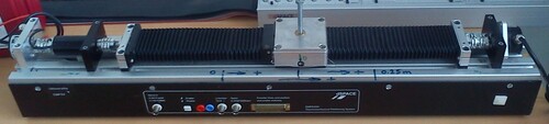
The EMPS is a standard component for robots or machine tools and is pictured in Figure 6. It is particularly difficult to identify, since it suffers from nonlinear, asymmetric friction. The input is the impulse force and the output is the position of the car.

Figure 6. Electro-mechanical positioning system setup (Janot et al., 2019).

The measurements and results for both configurations and for both activation functions are presented in Figure 7. The figures on the left correspond to the training data and the figures on the right correspond to the test data. The first two rows represent the output in the simulation configuration: black corresponds to the measured position, red to the simulated RKNN output using TANH, and blue to the simulated RKNN output utilising ReLU activation functions. As the deviation between measurement and estimation is not visible without zoom, the second row corresponds to the position error signal, $e_n=y_n-{\hat{y}}_{RKNN,n}$. The third and fourth rows present the results for the EMPS in prediction configuration and are displayed in an identical form as the simulation case in the first two rows. The fifth row depicts the complete force input signal and the sixth row presents an exemplary zoom on the force input for a given time interval.

Figure 7. Results on the EMPS benchmark, for training and test data, both activation functions and both configurations. All results are ISS stable. The training case is displayed on the left and the test scenario on the right. The y-axis description of each row is identical and the x-axis description in all cases is the time in seconds. Black lines correspond to measurements, red lines to RKNN with TANH and blue lines to RKNN with ReLU. The first two rows refer to the simulation configuration and the third and fourth rows to the prediction configuration. The fifth and sixth row display the force input signal.

The figure shows that the RKNN can satisfactorily simulate (first row) and predict (third row) the benchmark. As almost no difference between the measurements $y_n$ and the model output ${\hat{y}}_{RKNN,n}$ can be observed without magnification, the second and fourth rows represent the output error $e_n=y_n-{\hat{y}}_{RKNN,n}$.

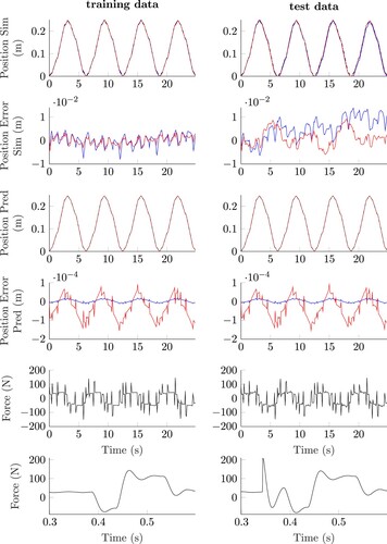
As expected, the prediction configuration outperforms the simulation configuration by 2 orders of magnitude. For both, training and test data, the RKNN achieves a similar performance, demonstration sufficient generalisation capabilities. In prediction configuration, the ReLU activation function outperforms the RKNN with TANH activation. The results for EMPS are computed on the original time grid, without interpolation or time-domain normalisation.

Only few other black-box identification algorithms for this benchmark have been published yet. Forgione and Piga (2021b) develops a neural network called dynoNet with linear dynamics operators as elementary building blocks. Instead of activation functions, a transfer function is applied in each neuron.³ Janot et al. (2019) identify a best linear fit with the CAPTAIN and the CONTSID toolboxes.⁴ Most importantly, Forgione and Piga (2021a) identified continuous-time neural networks for the EMPS and the Cascaded Tank benchmark in simulation configuration. Fortunately, Forgione's paper was published while this work was still in the review process as it is a direct comparison to RKNN. Forgione discusses various integration methods including RK and enhances the system identification with a soft-constrained integration method (SCI) and a truncated simulation error minimisation (TSEM). Regarding the EMPS benchmark, Forgione included few physical knowledge into the neural network structure.⁵ A comparison of the results is presented in Table 1.

Table 1. Results on the EMPS benchmark in prediction (Pred) and simulation (Sim) configuration. RKNN is ISS stable. Complete evaluation metrics are given in Appendix A. See main text for references. Note that the data unit is m and RMSE unit is mm.

	Test $e_{RMSE}$ (mm)
best linear fit Sim	111.10
Truncated simulation error minimisation (TSEM) Sim	4.73
Soft-constrained integration method (SCI) Sim	6.65
RKNN Sim (ours)	3.68
RKNN Pred (ours)	0.0087

Table 1 reveals that continuous-time methods (TSEM, SCI and RKNN) can improve the RMSE compared to the best linear fit by a factor of 20. In prediction configuration, we are pleased to report the first results in the micrometre scale, although there is no black-box comparison published yet. Hopefully, more black-box methods will consider this benchmark in the future. However, great results on this application can be archived using hard-crafted grey-box approaches (Chaves Ferreira Pinto & Hultmann Ayala, 2020; Janot et al., 2019, 2017).

7.3. Cascaded tanks

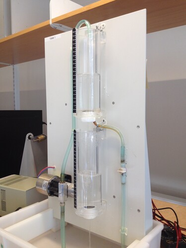
Schoukens et al. (2016) wrote that ‘the cascaded tanks system is a fluid level control system consisting of two tanks with free outlets fed by a pump. The input signal controls a water pump that pumps the water from a reservoir into the upper water tank. The water of the upper water tank flows through a small opening into the lower water tank, and finally through a small opening from the lower water tank back into the reservoir’. The three tank setup is depicted in Figure 8.

Figure 8. Cascaded Tank Setup. Schoukens et al. (2016).

The system exhibits weakly nonlinear behaviour during normal operation and hard saturation effects, when the tank overflows, depending on the input. As presented by Schoukens et al. (2016), the dynamics in continuous time of the three tanks without the overflow effect are given by (16a) $\begin{array}{rl}{\dot{x}}_1\left(t\right)& =-k_1\sqrt{x_1\left(t\right)}+k_{4}u\left(t\right)+w_1\left(t\right),\end{array}$(16a) (16b) $\begin{array}{rl}{\dot{x}}_2\left(t\right)& =k_2\sqrt{x_1\left(t\right)}-k_3\sqrt{x_2\left(t\right)}+w_2\left(t\right),\end{array}$(16b) (16c) $\begin{array}{rl}y\left(t\right)& =x_2\left(t\right)+e\left(t\right),\end{array}$(16c)

with scalar damping coefficients $k_1$,$k_2$,$k_3$,$k_4$, noise $w_1\left(t\right),w_2\left(t\right),e\left(t\right)$ and states, input and output as defined before.

As the benchmark exhibits a large sample time, we test for both time-domain interpolation (RKNN with INT, Figure 9) and time-domain normalisation (RKNN with TDN, Figure 10). Regarding the interpolation, a zero-order-hold element for several time steps is included in training and validation. As a consequence, the sample time can be reduced from 4000 ms to 400 ms by holding the same input ${\tilde{u}}_n$ and state $x_n$ for 10 time steps. For improved comparison, we chose zero-order-hold instead of advanced interpolation schemes to avoid an augmentation of the data, as some methods in literature struggle with an identification using only 1024 data points. As a comprehensive consequence, the simulation horizon increases to 10240 time steps. Regarding the time-domain normalisation, the normalised sample time is set to $h_{norm}=40$ ms and 1024 data points are employed. The results are evaluated on the original time grid with N = 1024 and $h_{data}=4000$ ms in both cases.

Figure 9. Results on the Cascaded Tank benchmark, using interpolation, for training and test data, both activation functions and both configurations. All results are ISS stable. The training case is displayed on the left and the test scenario on the right. The y-axis description of each row is identical and the x-axis description in all cases is the time in seconds. This figure applies the same y-axis scaling as Figure 10. Black lines correspond to measurements, red lines to RKNN with TANH and blue lines to RKNN with ReLU. The first two rows refer to the simulation configuration and the third and fourth rows to the prediction configuration. The fifth and sixth rows display the input signal.

The figure shows that the RKNN can satisfactorily simulate (first row) and predict (third row) the benchmark. To display the difference between the measurements $y_n$ and the estimation ${\hat{y}}_{RKNN,n}$ in more detail, the second and fourth rows represent the output error $e_n=y_n-{\hat{y}}_{RKNN,n}$.

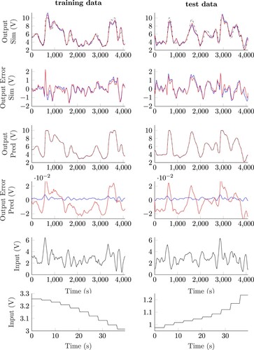
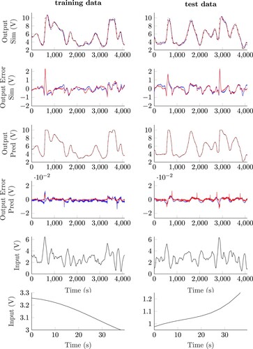
Figure 10. Results on the Cascaded Tank benchmark, using time-domain normalisation, for training and test data, both activation functions and both configurations. All results are ISS stable. The training case is displayed on the left and the test scenario on the right. The y-axis description of each row is identical and the x-axis description in all cases is the time in seconds. This figure applies the same y-axis scaling as Figure 9. Black lines correspond to measurements, red lines to RKNN with TANH and blue lines to RKNN with ReLU. The first two rows refer to the simulation configuration and the third and fourth rows to the prediction configuration. The fifth and sixth row display the input signal.

The figure shows that the RKNN can satisfactorily simulate (first row) and predict (third row) the benchmark. To display the difference between the measurements $y_n$ and the estimation ${\hat{y}}_{RKNN,n}$ in more detail, the second and fourth rows represent the output error $e_n=y_n-{\hat{y}}_{RKNN,n}$.

In the literature, many nonlinear methods have addressed the Cascaded Tank benchmark. We will start with the approaches that have delivered the best results in prediction configuration at the time of this publication. Belz et al. (2017) apply local model networks with external dynamics to the benchmark problem, represented by three different approaches: NARX, NFIR and NOBF components. Aljamaan et al. (2021) develop a Hammerstein Box–Jenkins model for the identification benchmark. Worden et al. (2018) presents a record of participants of the nonlinear system identification workshop considering this benchmark among others. White, grey and black box approaches are discussed and evolutionary algorithms are applied for system identification in both prediction and simulation configuration.⁶ Hostettler et al. (2018) propose a Gaussian Process-based nonlinear, time-varying drift model for stochastic differential equations. Results are compared in Table 2 and the complete evaluation metrics are given in Appendix A. To the best of our knowledge, the RKNN with time-domain normalisation and provable ISS stability is capable of outperforming all published methods by a factor of 10.

Table 2. Results on the Cascaded Tank benchmark in prediction configuration. RKNN is ISS stable. Complete evaluation metrics are given in the Appendix A. See main text for references.

	Test data $e_{RMSE}$ (V)
Local model networks	0.0207
Evolutionary algorithms	0.0515
Hammerstein Box-Jenkins	0.0671
Gaussian drift model	0.0576
RKNN with INT (ours)	0.0026
RKNN with TDN (ours)	0.0021

Figures 9 and 10, as well as Table 2, present an unexpected good performance in prediction configuration. From physical insight, as both tanks are independent, the two states should be independent, too. Therefore, we expected the application of the output derivative as a second state to be problematic. The RKNN in prediction configuration addressed this challenge successfully.

Many nonlinear methods addressed Cascaded Tank benchmark in the more sophisticated simulation configuration. We cannot refer to all approaches, so we will discuss the ones with the best results regarding RMSE in simulation configuration. Svensson and Schön (2017) wrote that it is ‘surprisingly hard to perform better than linear models in this problem, perhaps because of the close-to-linear dynamics in most regimes, in combination with the non-smooth overflow events’. The overflows occur only in a few time steps and completely changes the dynamical behaviour of the system. Svensson develops a flexible, nonlinear state–space model with a Gaussian–Process inspired prior. As discussed in Section 7.2, Forgione and Piga (2021a) develop the SCI and TSEM methods as direct comparison to RKNN. Another direct comparison is called integrated neural networks (INN) by Mavkov et al. (2020) which applies continuous-time neural networks with the Euler integration scheme. The best linear approximation is given in Relan et al. (2017). Furthermore, Relan et al. (2017) designs an unstructured flexible nonlinear state space model with different initialisation schemes (nonlinear SS with NLSS2 initialisation). Birpoutsoukis et al. (2018) develop a truncated volterra series model for the benchmark and extend its regularisation method. All methods are compared in Table 3.

Table 3. Results on the Cascaded Tank benchmark in simulation configuration with time-domain normalisation. RKNN is ISS stable. Complete evaluation metrics are given in the Appendix A. See main text for references.

	Test data $e_{RMSE}$ (V)
Best linear approximation	0.75
State-space with GP-inspired prior	0.45
Evolutionary algorithms	0.47
Nonlinear SS with NLSS2 initialisation	0.34
Truncated volterra model	0.54
Truncated simulation error minimisation (TSEM)	0.33
Soft-constrained integration method (SCI)	0.40
Integrated neural networks (INN)	0.41
RKNN with INT (ours)	0.61
RKNN with TDN (ours)	0.39

All in all, the RKNN with ISS provides a comprehensive RMSE in simulation and prediction configuration on this benchmark. Especially the direct comparison with the methods using continuous-time neural networks, TSEM, SCI and INN, presents a similar performance. Table 3 demonstrates that time-continuous neural networks (TSEM, SCI, INN and RKNN) are comprehensive methods compared with approaches beyond neural networks. TSEM provides the best RMSE on this benchmark in simulation. It should be pointed out that none of the discussed works considered ISS stability. Therefore, we conclude that the ISS stability constraints are not too conservative. Note that many more nonlinear methods have been applied to this benchmark, we only referred to the ones leading the field. To the best of our knowledge, the RKNN with ISS provides the best results for both benchmarks in prediction configuration in the literature. An improvement of accuracy can be achieved of factor 10 in prediction configuration. Furthermore, the similar approach also using continuous-time neural networks, TSEM, is leading the Cascaded Tank benchmark in simulation configuration.

8. Conclusion

In this contribution, input-to-state stability (ISS) of continuous-time neural networks discretised by explicit Runge–Kutta methods (RKNN) is investigated. The ISS property for RKNN extends the stability results from control theory to neural networks. Especially for industrial applications, it is important to prove that all predicted states remain bounded in every potential use case and under all possible circumstances. The drawback is that constraints always narrow the solution space. Nevertheless, RKNN keeps full nonlinear black-box identification capabilities. Furthermore, the presented stability guarantee already holds during training. The constraints rely only on the weights of the neural network and are not dependant on any measurement or any handcrafted physical insight of the process.

A future research is required to combine the ISS stable neural network with control, i.e. how to include the RKNN in a model-based reinforcement learning (RL) algorithm or in a model predictive controller (MPC). First steps of combining control with RKNN have been done by Weigand et al. (2020) for model-based RL and by Uçak (2020) for MPC. Another promising direction is further analysis of time-domain normalisation (TDN), i.e. developing auto-tuning mechanisms for TDN.

Acknowledgments

We thank Vassilios Yfantis, Patrick Bachmann, Achim Wagner and the anonymous reviewers for providing substantial comments on the manuscript.

Disclosure statement

No potential conflict of interest was reported by the author(s).

Additional information

Funding

This research was supported by the project RACKET under grant 01IW20009 by the German Federal Ministry of Education and Research.

Notes

1 We refer to variable sample time between data sets, i.e. training and application, and not within one data set.

2 Both theorems guarantee stability even for a large sample time. In this case, the constraints force the network to reduce its dynamic, until the simulation of the RKNN remains close to the origin for all time steps.

3 Direct communication with the authors revealed that the RMSE might have an unit error. We encourage reading the paper.

4 The paper only states the relative error $e_{rel,sim}=74$ %. We estimated the corresponding RMSE in Table 1 with $e_{RMSE}=(e_{rel}\parallel y_{meas}{\parallel }_2)/\left(\sqrt{N}100\right)$.

5 The results for the EMPS benchmark origin from direct contact to the authors. The authors report for the TSEM method $R^2=0.9967,e_{RMSE}=4.7253$ mm and for the SCI method $R^2=0.9935,e_{RMSE}=6.646$ mm. Results for the Cascaded Tank benchmark are given the paper.

6 The paper only states the best normalised mean squared error (NMSE) of $e_{NMSE,pred}=0.0565$ V and $e_{NMSE,sim}=4.6174$ V. We estimated the corresponding RMSE in Tables 2 and 3 with $e_{RMSE}=\sqrt{e_{NMSE}{\sigma }_y^2/100}$

Appendix A.

Complete evaluation metrics

Evaluation metrics are defined in Section 7.1 and are presented in Table A1, Table A2 and Table A3. For the EMPS metrics, note that the RMSE is given in mm while the data is given in m. Nomenclature:

RKNN	=	Runge–Kutta neural network
Sim	=	Simulation configuration
Pred	=	Prediction configuration
TANH	=	Hyperbolic tangent activation function
ReLU	=	Rectified linear unit activation function
Train	=	Training data set of the benchmark
Test	=	Test data set of the benchmark
INT	=	Time-domain interpolation
TDN	=	Time-domain normalisation

Table A1. Complete evaluation metrics on the EMPS benchmark. All results are ISS stable. Original time grid is applied.

	Train $e_{RMSE}$ mm	Train $e_{rel}$ %	Train $\mathit{f}\mathit{i}\mathit{t}$ %	Train $R^2$ %	Test $e_{RMSE}$ mm	Test $e_{rel}$ %	Test $\mathit{f}\mathit{i}\mathit{t}$ %	Test $R^2$ %
RKNN Sim ReLU	2.3475	1.58	97.16	99.92	6.9916	4.70	91.56	99.29
RKNN Sim TANH	1.7062	1.15	97.94	99.96	3.6917	2.48	95.53	99.80
RKNN Pred ReLU	0.0086	0.01	99.99	100.00	0.0086	0.01	99.99	100.00
RKNN Pred TANH	0.0670	0.04	99.92	100.00	0.0670	0.05	99.92	100.00

Appendix B.

Exemplary weights of the RKNN

For validation, we present the complete neural network weights $W^{H,l},W^l,W_a^o,W^h$ and the stability matrix $P_1$ for one of the presented cases. The following are the weights of the first case in Appendix A which is the RKNN with ReLU for the EMPS data set in simulation configuration. To save space, we do not present the complete weights for all 12 cases in this paper. Feel free to contact the authors if further information is required. Evaluation metrics for all 12 cases are given in Appendix A.

Table A2. Complete evaluation metrics on the Cascaded Tank benchmark. All results are ISS stable. Interpolation is applied (INT).

	Train $e_{RMSE}$ mm	Train $e_{rel}$ %	Train $\mathit{f}\mathit{i}\mathit{t}$ %	Train $R^2$ %	Test $e_{RMSE}$ mm	Test $e_{rel}$ %	Test $\mathit{f}\mathit{i}\mathit{t}$ %	Test $R^2$ %
RKNN Sim ReLU	0.5812	9.71	73.15	92.79	0.7026	11.50	66.54	88.80
RKNN Sim TANH	0.5414	9.04	74.98	93.74	0.6111	10.00	70.90	91.53
RKNN Pred ReLU	0.0026	0.04	99.88	100.00	0.0026	0.04	99.88	100.00
RKNN Pred TANH	0.0142	0.24	99.35	100.00	0.0133	0.22	99.36	100.00

The network is ISS stable. The maximum eigenvalue of all stability (sub)matrices $T_1,T_{2,i},\mathrm{\forall }i\in \{1,2,\dots ,N_N\}$ is $-304.1163$ and clearly less than zero (submatrices are relevant due to Sylvester's criterion). Note how few parameters the presented network architecture features compared to approaches in the literature. $\begin{array}{rl}{P}_1& =\left[\begin{array}{cc}182.5413& 89.2340\\ 89.2340& 86.8726\end{array}\right]>0\\ W^{H,l}& =\left[\begin{array}{cc}-1.2899& 0.9157\end{array}\right]\\ W^l& =\left[\begin{array}{ccc}-1.7053& -1.3739& -0.1200\\ -0.0825& -1.1882& 0.3541\end{array}\right]\\ W_a^o& =\left[\begin{array}{cccc}-1.5890& 1.1966& -1.3893& -1.0626\\ -0.2966& 1.3074& -1.0411& -1.3813\end{array}\right]\\ W^h& =\left[\begin{array}{cccc}0.5015& 1.4377& -0.2094& -0.2226\\ -0.5136& -1.2967& 0.5782& 1.0720\\ 1.3682& -0.8469& 0.0111& -0.0918\\ 1.2837& -0.7759& -0.4493& 0.7915\end{array}\right]\end{array}$

Appendix C.

Proof of Theorem

The idea of the proof is to find an estimation for (14(13) $〈x,f_{\mathrm{N}\mathrm{N}}(\hat{x},\tilde{u}){〉}_{P_1}+hm〈f_{\mathrm{N}\mathrm{N}}(\hat{x},\tilde{u}),f_{\mathrm{N}\mathrm{N}}(\hat{x},\tilde{u}){〉}_{P_1}<\gamma 〈\tilde{u},\tilde{u}〉$(13) ), such that linear matrix inequalities (LMI) only depend on the network weights and fixed parameters. First, we estimate the terms X and U. Then, we eliminate L. For the sake of simplicity, we set $X=W_x^l+W_a^{o}L{W}_x^h$ and $U=W_u^l+W_a^{o}L{W}_u^h$ to define $f_{\mathrm{N}\mathrm{N}}(\hat{x},\tilde{u})=Xx+U\tilde{u}$. We calculate the left-hand side of (14(13) $〈x,f_{\mathrm{N}\mathrm{N}}(\hat{x},\tilde{u}){〉}_{P_1}+hm〈f_{\mathrm{N}\mathrm{N}}(\hat{x},\tilde{u}),f_{\mathrm{N}\mathrm{N}}(\hat{x},\tilde{u}){〉}_{P_1}<\gamma 〈\tilde{u},\tilde{u}〉$(13) ) by (A1) $\begin{array}{rl}& 〈x,f_{\mathrm{N}\mathrm{N}}(\hat{x},\tilde{u}){〉}_{P_1}+hm〈f_{\mathrm{N}\mathrm{N}}(\hat{x},\tilde{u}),f_{\mathrm{N}\mathrm{N}}(\hat{x},\tilde{u}){〉}_{P_1}\\ & =x^T{P}_1(Xx+U\tilde{u})+hm\left(\right(Xx+U\tilde{u}{)}^T{P}_1(Xx+U\tilde{u}))\\ & =x^T(P_{1}X+hm{X}^T{P}_{1}X)x+x^T(P_{1}U+2hm{X}^T{P}_{1}U)\tilde{u}\\ & +{\tilde{u}}^T\left(hm{U}^T{P}_{1}U\right)\tilde{u}.\end{array}$(A1) To estimate the term $x^T(P_{1}U+2hm{X}^T{P}_{1}U)\tilde{u}$, we use the general relation $2z_1^T{z}_2\le z_1^T{P}_2{z}_1+z_2^T{P}_2^{-1}{z}_2$ which is valid for any vectors $z_1,z_2\in {\mathbb{R}}^{N_X}$ and for any positive definite matrix $P_2>0,P_2\in {\mathbb{R}}^{N_X\times N_X}$ (Horn & Johnson, 2012: Theorem 7.7.6 and 7.7.7). (A2) $\begin{array}{rl}& x^T(P_{1}U+2hm{X}^T{P}_{1}U)\tilde{u}\\ & =2\left(\frac{1}{2}x{)}^T\right(P_{1}U\tilde{u})+2(x{)}^T\left(hm{X}^T{P}_{1}U\tilde{u}\right)\\ & \le \left(\frac{1}{2}x{)}^T{P}_2\right(\frac{1}{2}x)+(P_{1}U\tilde{u}{)}^T{P}_2^{-1}\left(P_{1}U\tilde{u}\right)\\ & +x^T{P}_{2}x+\left(hm{X}^T{P}_{1}U\tilde{u}{)}^T{P}_2^{-1}\right(hm{X}^T{P}_{1}U\tilde{u})\\ & =\frac{5}{4}{x}^T{P}_{2}x\\ & +{\tilde{u}}^T(U^T{P}_1^T\cdot (P_2^{-1}+h^2{m}^{2}X{P}_2^{-1}{X}^T\left)P_{1}U\right)\tilde{u}.\end{array}$(A2) Substituting (A2(A2) $\begin{array}{rl}& x^T(P_{1}U+2hm{X}^T{P}_{1}U)\tilde{u}\\ & =2\left(\frac{1}{2}x{)}^T\right(P_{1}U\tilde{u})+2(x{)}^T\left(hm{X}^T{P}_{1}U\tilde{u}\right)\\ & \le \left(\frac{1}{2}x{)}^T{P}_2\right(\frac{1}{2}x)+(P_{1}U\tilde{u}{)}^T{P}_2^{-1}\left(P_{1}U\tilde{u}\right)\\ & +x^T{P}_{2}x+\left(hm{X}^T{P}_{1}U\tilde{u}{)}^T{P}_2^{-1}\right(hm{X}^T{P}_{1}U\tilde{u})\\ & =\frac{5}{4}{x}^T{P}_{2}x\\ & +{\tilde{u}}^T(U^T{P}_1^T\cdot (P_2^{-1}+h^2{m}^{2}X{P}_2^{-1}{X}^T\left)P_{1}U\right)\tilde{u}.\end{array}$(A2) ) in (A1(A1) $\begin{array}{rl}& 〈x,f_{\mathrm{N}\mathrm{N}}(\hat{x},\tilde{u}){〉}_{P_1}+hm〈f_{\mathrm{N}\mathrm{N}}(\hat{x},\tilde{u}),f_{\mathrm{N}\mathrm{N}}(\hat{x},\tilde{u}){〉}_{P_1}\\ & =x^T{P}_1(Xx+U\tilde{u})+hm\left(\right(Xx+U\tilde{u}{)}^T{P}_1(Xx+U\tilde{u}))\\ & =x^T(P_{1}X+hm{X}^T{P}_{1}X)x+x^T(P_{1}U+2hm{X}^T{P}_{1}U)\tilde{u}\\ & +{\tilde{u}}^T\left(hm{U}^T{P}_{1}U\right)\tilde{u}.\end{array}$(A1) ) leads to (A3) $\begin{array}{rl}& 〈x,f_{\mathrm{N}\mathrm{N}}(\hat{x},\tilde{u}){〉}_{P_1}+hm〈f_{\mathrm{N}\mathrm{N}}(\hat{x},\tilde{u}),f_{\mathrm{N}\mathrm{N}}(\hat{x},\tilde{u}){〉}_{P_1}\\ & \le x^T(\frac{5}{4}{P}_2+P_{1}X+hm{X}^T{P}_{1}X)x\\ & +{\tilde{u}}^T\left(U^T\right(hm{P}_1+P_1^T{P}_2^{-1}{P}_1\\ & +h^2{m}^2{P}_1^{T}X{P}_2^{-1}{X}^T{P}_1\left)U\right)\tilde{u}.\\ & <\gamma 〈\tilde{u},\tilde{u}〉\end{array}$(A3) We fulfil (A3(A3) $\begin{array}{rl}& 〈x,f_{\mathrm{N}\mathrm{N}}(\hat{x},\tilde{u}){〉}_{P_1}+hm〈f_{\mathrm{N}\mathrm{N}}(\hat{x},\tilde{u}),f_{\mathrm{N}\mathrm{N}}(\hat{x},\tilde{u}){〉}_{P_1}\\ & \le x^T(\frac{5}{4}{P}_2+P_{1}X+hm{X}^T{P}_{1}X)x\\ & +{\tilde{u}}^T\left(U^T\right(hm{P}_1+P_1^T{P}_2^{-1}{P}_1\\ & +h^2{m}^2{P}_1^{T}X{P}_2^{-1}{X}^T{P}_1\left)U\right)\tilde{u}.\\ & <\gamma 〈\tilde{u},\tilde{u}〉\end{array}$(A3) ) and thereby Theorem 5.2 in two steps. First, we show that all terms in (A3(A3) $\begin{array}{rl}& 〈x,f_{\mathrm{N}\mathrm{N}}(\hat{x},\tilde{u}){〉}_{P_1}+hm〈f_{\mathrm{N}\mathrm{N}}(\hat{x},\tilde{u}),f_{\mathrm{N}\mathrm{N}}(\hat{x},\tilde{u}){〉}_{P_1}\\ & \le x^T(\frac{5}{4}{P}_2+P_{1}X+hm{X}^T{P}_{1}X)x\\ & +{\tilde{u}}^T\left(U^T\right(hm{P}_1+P_1^T{P}_2^{-1}{P}_1\\ & +h^2{m}^2{P}_1^{T}X{P}_2^{-1}{X}^T{P}_1\left)U\right)\tilde{u}.\\ & <\gamma 〈\tilde{u},\tilde{u}〉\end{array}$(A3) ) associated with $\tilde{u}$ are lower bounded by a function $\gamma 〈\tilde{u},\tilde{u}〉\ge 0$. Second, we ensure that the terms associated with x are strictly negative. The positive function for any input $\tilde{u}$ and any state x is given by (A4) $\begin{array}{rl}\gamma 〈\tilde{u},\tilde{u}〉& =\underset{x,\tilde{u}}{min}\parallel \left(U\right(x,\tilde{u}\left){)}^T\right(hm{P}_1+P_1^T{P}_2^{-1}{P}_1\\ & +h^2{m}^2{P}_1^{T}X(x,\tilde{u})P_2^{-1}\left(X\right(x,\tilde{u}\left){)}^T{P}_1\right)U(x,\tilde{u})\parallel \ge 0.\end{array}$(A4) Equation (A4(A4) $\begin{array}{rl}\gamma 〈\tilde{u},\tilde{u}〉& =\underset{x,\tilde{u}}{min}\parallel \left(U\right(x,\tilde{u}\left){)}^T\right(hm{P}_1+P_1^T{P}_2^{-1}{P}_1\\ & +h^2{m}^2{P}_1^{T}X(x,\tilde{u})P_2^{-1}\left(X\right(x,\tilde{u}\left){)}^T{P}_1\right)U(x,\tilde{u})\parallel \ge 0.\end{array}$(A4) ) holds always true as the norm is by definition greater or equal than zero. To ensure that the terms in (A3(A3) $\begin{array}{rl}& 〈x,f_{\mathrm{N}\mathrm{N}}(\hat{x},\tilde{u}){〉}_{P_1}+hm〈f_{\mathrm{N}\mathrm{N}}(\hat{x},\tilde{u}),f_{\mathrm{N}\mathrm{N}}(\hat{x},\tilde{u}){〉}_{P_1}\\ & \le x^T(\frac{5}{4}{P}_2+P_{1}X+hm{X}^T{P}_{1}X)x\\ & +{\tilde{u}}^T\left(U^T\right(hm{P}_1+P_1^T{P}_2^{-1}{P}_1\\ & +h^2{m}^2{P}_1^{T}X{P}_2^{-1}{X}^T{P}_1\left)U\right)\tilde{u}.\\ & <\gamma 〈\tilde{u},\tilde{u}〉\end{array}$(A3) ) associated with the state x are strictly less than zero, we define (A5) $Z_1=\frac{5}{4}{P}_2+P_{1}X+hm{X}^T{P}_{1}X.$(A5) We resubstitute X and calculate (A6) $\begin{array}{rl}{X}^T{P}_{1}X& =(W_x^l+W_a^{o}L{W}_x^h{)}^T{P}_1(W_x^l+W_a^{o}L{W}_x^h)\\ & ={W_x^l}^T{P}_1{W}_x^l+{W_x^l}^T{P}_1{W}_a^{o}L{W}_x^h\\ & +(W_a^{o}L{W}_x^h{)}^T{P}_1{W}_x^l\\ & +(W_a^{o}L{W}_x^h{)}^T{P}_1{W}_a^{o}L{W}_x^h.\end{array}$(A6) Next, we eliminate L in two steps. We know that $\parallel L\parallel \le 1$ holds and estimate the positive definite term (A7) $\begin{array}{rl}& x^T(W_a^{o}L{W}_x^h{)}^T{P}_1{W}_a^{o}L{W}_x^{h}x\le x^{T}Qx,\\ & Q=\parallel {W_a^o}^T{P}_1{W}_a^o\parallel \parallel W_x^h{\parallel }^{2}I.\end{array}$(A7) Using (A7(A7) $\begin{array}{rl}& x^T(W_a^{o}L{W}_x^h{)}^T{P}_1{W}_a^{o}L{W}_x^{h}x\le x^{T}Qx,\\ & Q=\parallel {W_a^o}^T{P}_1{W}_a^o\parallel \parallel W_x^h{\parallel }^{2}I.\end{array}$(A7) ) in (A6(A6) $\begin{array}{rl}{X}^T{P}_{1}X& =(W_x^l+W_a^{o}L{W}_x^h{)}^T{P}_1(W_x^l+W_a^{o}L{W}_x^h)\\ & ={W_x^l}^T{P}_1{W}_x^l+{W_x^l}^T{P}_1{W}_a^{o}L{W}_x^h\\ & +(W_a^{o}L{W}_x^h{)}^T{P}_1{W}_x^l\\ & +(W_a^{o}L{W}_x^h{)}^T{P}_1{W}_a^{o}L{W}_x^h.\end{array}$(A6) ) we get (A8) $\begin{array}{rl}{X}^T{P}_{1}X& \le {W_x^l}^T{P}_1{W}_x^l+{W_x^l}^T{P}_1{W}_a^{o}L{W}_x^h\\ & +(W_a^{o}L{W}_x^h{)}^T{P}_1{W}_x^l+Q.\end{array}$(A8) Substitution of (A8(A8) $\begin{array}{rl}{X}^T{P}_{1}X& \le {W_x^l}^T{P}_1{W}_x^l+{W_x^l}^T{P}_1{W}_a^{o}L{W}_x^h\\ & +(W_a^{o}L{W}_x^h{)}^T{P}_1{W}_x^l+Q.\end{array}$(A8) ) in (A5(A5) $Z_1=\frac{5}{4}{P}_2+P_{1}X+hm{X}^T{P}_{1}X.$(A5) ) leads to $\begin{array}{rl}{x}^T{Z}_{1}x& \le x^T(P_3+P_1{W}_x^l+P_1{W}_a^{o}L{W}_x^h\\ & +hm({W_x^l}^T{P}_1{W}_x^l+{W_x^l}^T{P}_1{W}_a^{o}L{W}_x^h\\ & +(W_a^{o}L{W}_x^h{)}^T{P}_1{W}_x^l+Q))x\\ & =x^T(T_1+(hm{W_x^l}^T+I)P_1{W}_a^{o}L{W}_x^h\\ & +hm\left(W_a^{o}L{W}_x^h{)}^T{P}_1{W}_x^l\right))x\\ & =x^T{Z}_{2}x\end{array}$

Table A3. Complete evaluation metrics on the Cascaded Tank benchmark. All results are ISS stable. Time-domain normalisation is applied (TDN).

	Train $e_{RMSE}$ mm	Train $e_{rel}$ %	Train $\mathit{f}\mathit{i}\mathit{t}$ %	Train $R^2$ %	Test $e_{RMSE}$ mm	Test $e_{rel}$ %	Test $\mathit{f}\mathit{i}\mathit{t}$ %	Test $R^2$ %
RKNN Sim ReLU	0.3485	5.82	83.90	97.41	0.4233	6.93	79.84	95.94
RKNN Sim TANH	0.3518	5.87	83.75	97.36	0.3906	6.39	81.39	96.54
RKNN Pred ReLU	0.0024	0.04	99.89	100.00	0.0026	0.04	99.88	100.00
RKNN Pred TANH	0.0011	0.02	99.95	100.00	0.0021	0.03	99.90	100.00

with $T_1=P_3+P_1{W}_x^l+hm({W_x^l}^T{P}_1{W}_x^l+Q).$ Then, to estimate the other terms independently of L we follow the approach in Hu and Wang (2002a). We define the ith row vector of matrix $W_x^h$ as $R_i^{Wh}$ and the ith column vector of matrix $W_a^o$ as $C_i^{Wo}$ and obtain $W_a^{o}L{W}_x^h=\sum _{i=1}^{N_N}{l}_i{C}_i^{Wo}{R}_i^{Wh}.$ Consequently, we can estimate $\begin{array}{rl}{x}^T{Z}_{2}x& =x^T\left(T_1+(hm{W_x^l}^T+I)P_1\sum _{i=1}^{N_N}{l}_i{C}_i^{Wo}{R}_i^{Wh}\right.\\ & +\left.hm{\left(\sum _{i=1}^{N_N}{l}_i{C}_i^{Wo}{R}_i^{Wh}\right)}^T{P}_1{W}_x^l\right)x\\ & =x^T\left(T_1+\sum _{i=1}^{N_N}{l}_i\left(\right(hm{W_x^l}^T+I)P_1{C}_i^{Wo}{R}_i^{Wh}\right.\\ & +hm\left(C_i^{Wo}{R}_i^{Wh}{)}^T{P}_1{W}_x^l\right)\left.\phantom{\sum _{i=1}^{N_N}}\right)x\\ & =x^T{Z}_{3}x.\end{array}$ Introducing the weighting variables ${\lambda }_i$, with $\sum _{i=1}^{N_N}{\lambda }_i=1,0\le {\lambda }_i\le 1,\mathrm{\forall }i\in \{1,\dots ,N_N\}$ we can reformulate $T_1$ (A9) $T_1=\left(1-\sum _{i=1}^{N_N}{l}_i{\lambda }_i\right)T_1+\left(\sum _{i=1}^{N_N}{l}_i{\lambda }_i\right)T_1$(A9) Incorporating (A9(A9) $T_1=\left(1-\sum _{i=1}^{N_N}{l}_i{\lambda }_i\right)T_1+\left(\sum _{i=1}^{N_N}{l}_i{\lambda }_i\right)T_1$(A9) ) into the sum leads to $\begin{array}{rl}{x}^T{Z}_{3}x& =x^T\left(1-\sum _{i=1}^{N_N}{l}_i{\lambda }_i\right)T_{1}x\\ & +\sum _{i=1}^{N_N}{l}_i{x}^T\left(\right(hm{W_x^l}^T+I)P_1{C}_i^{Wo}{R}_i^{Wh}\\ & +hm(C_i^{Wo}{R}_i^{Wh}{)}^T{P}_1{W}_x^l+T_1{\lambda }_i)x\\ & =x^T\left(1-\sum _{i=1}^{N_N}{l}_i{\lambda }_i\right)T_{1}x+\sum _{i=1}^{N_N}{l}_i{x}^T(T_{2,i}+T_1{\lambda }_i)x.\end{array}$ with $\begin{array}{rl}{T}_{2,i}& =(hm{W_x^l}^T+I)P_1{C}_i^{Wo}{R}_i^{Wh}\\ & +hm(C_i^{Wo}{R}_i^{Wh}{)}^T{P}_1{W}_x^l.\end{array}$ By the definition of the weight variables ${\lambda }_i$ and the fact that $0\le l_i\le 1$ holds, we ensure that $\left(1-\sum _{i=1}^{N_N}{l}_i{\lambda }_i\right)\ge 0$ holds and the proof is completed.

References

- Ahmed, N. K., Atiya, A. F., Gayar, N. E., & El-Shishiny, H. (2010). An empirical comparison of machine learning models for time series forecasting. Econometric Reviews, 29(5–6), 594–621. https://doi.org/10.1080/07474938.2010.481556
- Aljamaan, I. A., Al-Dhaifallah, M. M., & Westwick, D. T. (2021). Hammerstein box-Jenkins system identification of the cascaded tanks benchmark system. Mathematical Problems in Engineering, 2021(6), 1–8. https://doi.org/10.1155/2021/6613425
- Barabanov, N. E., & Prokhorov, D. V. (2002). Stability analysis of discrete-time recurrent neural networks. IEEE Transactions on Neural Networks, 13(2), 292–303. https://doi.org/10.1109/72.991416
- Belz, J., Münker, T., Heinz, T. O., Kampmann, G., & Nelles, O. (2017). Automatic modeling with local model networks for benchmark processes. IFAC-PapersOnLine, 50(1), 470–475. https://doi.org/10.1016/j.ifacol.2017.08.089
- Birpoutsoukis, G., P. Z. Csurcsia, & Schoukens, J. (2018). Efficient multidimensional regularization for Volterra series estimation. Mechanical Systems and Signal Processing, 104(11), 896–914. https://doi.org/10.1016/j.ymssp.2017.10.007
- Butcher, J. C. (2016). Numerical methods for ordinary differential equations (3rd ed.). Wiley. https://doi.org/10.1002/9781119121534
- Byrd, R. H., Hribar, M. E., & Nocedal, J. (1999). An interior point algorithm for large-scale nonlinear programming. SIAM Journal on Optimization, 9(4), 877–900. https://doi.org/10.1137/S1052623497325107
- Chaves Ferreira Pinto, W., & Hultmann Ayala, H. V. (2020). Ensemble grey and black-box nonlinear system identification of a positioning system. Anais da Sociedade Brasileira de Automatica, 2(1), CBA2020. https://doi.org/10.48011/asba.v2i1.1570
- Chen, S., Billings, S. A., & Grant, P. M. (1990). Non-linear system identification using neural networks. International Journal of Control, 51(6), 1191–1214. https://doi.org/10.1080/00207179008934126
- Cooper, G. J. (1984). A generalization of algebraic stability for Runge–Kutta methods. IMA Journal of Numerical Analysis, 4(4), 427–440. https://doi.org/10.1093/imanum/4.4.427
- Deflorian, M. (2010). On Runge-Kutta neural networks: Training in series-parallel and parallel configuration. 49th IEEE Conference on Decision and Control (CDC) (pp. 4480–4485). https://doi.org/10.1109/CDC.2010.5717492
- Deflorian, M. (2011). Versuchsplanung und Methoden zur Identifikation zeitkontinuierlicher Zustandsraummodelle am Beispiel des Verbrennungsmotors [Dissertation]. Technische Universität München.
- Deflorian, M., Klöpper, F., & Rückert, J. (2010). Online dynamic black box modelling and adaptive experiment design in combustion engine calibration. IFAC Proceedings Volumes, 43(7), 703–708. https://doi.org/10.3182/20100712-3-DE-2013.00068
- Deflorian, M., & Rungger, M. (2014). Generalization of an input-to-state stability preserving Runge–Kutta method for nonlinear control systems. Journal of Computational and Applied Mathematics, 255(1), 346–352. https://doi.org/10.1016/j.cam.2013.05.017
- Efe, M. O., & Kaynak, O. (2000). A comparative study of soft-computing methodologies in identification of robotic manipulators. Robotics and Autonomous Systems, 30(3), 221–230. https://doi.org/10.1016/S0921-8890(99)00087-1
- Forgione, M., & Piga, D. (2021a). Continuous-time system identification with neural networks: Model structures and fitting criteria. European Journal of Control, 59(5), 69–81. https://doi.org/10.1016/j.ejcon.2021.01.008
- Forgione, M., & Piga, D. (2021b). dynoNet: a neural network architecture for learning dynamical systems. International Journal of Adaptive Control and Signal Processing, 35(4), 612–626. https://doi.org/10.1002/acs.v35.4
- Giorgio, G. (2017). Various proofs of the sylvester criterion for quadratic forms. Journal of Mathematics Research, 9(6), 55. https://doi.org/10.5539/jmr.v9n6p55
- Haykin, S. (1990). Neural networks – A comprehensive foundation. Prentice Hall.
- Horn, R. A., & Johnson, C. R. (2012). Matrix analysis (2nd ed.). Cambridge University Press.
- Hostettler, R., Tronarp, F., & Särkkä, S. (2018). Modeling the drift function in stochastic differential equations using reduced rank Gaussian processes. IFAC-PapersOnLine, 51(15), 778–783. https://doi.org/10.1016/j.ifacol.2018.09.137
- Hu, S., & Wang, J. (2002a). Global stability of a class of continuous-time recurrent neural networks. IEEE Transactions on Circuits and Systems I: Fundamental Theory and Applications, 49(9), 1334–1347. https://doi.org/10.1109/TCSI.2002.802360
- Hu, S., & Wang, J. (2002b). Global stability of a class of discrete-time recurrent neural networks. IEEE Transactions on Circuits and Systems I: Fundamental Theory and Applications, 49(8), 1104–1117. https://doi.org/10.1109/TCSI.2002.801284
- Janot, A., Gautier, M., & Brunot, M. (2019). Data Set and Reference Models of EMPS. 2019 Workshop on Nonlinear System Identification Benchmarks, Eindhoven, The Netherlands.
- Janot, A., Young, P. C., & Gautier, M. (2017). Identification and control of electro-mechanical systems using state-dependent parameter estimation. International Journal of Control, 90(4), 643–660. https://doi.org/10.1080/00207179.2016.1209565
- Jiang, Z. P.., & Wang, Y. (2001). Input-to-state stability for discrete-time nonlinear systems. Automatica, 37(6), 857–869. https://doi.org/10.1016/S0005-1098(01)00028-0
- Khalil, H. K. (2002). Nonlinear systems (3rd ed.). Prentice Hall.
- Mavkov, B., Forgione, M., & Piga, D. (2020). Integrated neural networks for nonlinear continuous-time system identification. IEEE Control Systems Letters, 4(4), 851–856. https://doi.org/10.1109/LCSYS.2020.2994806
- Narendra, K., & Parthasarathy, K. (1990). Identification and control of dynamical systems using neural networks. IEEE Transactions on Neural Networks, 1(1), 4–27. https://doi.org/10.1109/72.80202
- Nelles, O. (2001). Nonlinear system identification. Springer Verlag.
- Relan, R., Tiels, K., Marconato, A., & Schoukens, J. (2017). An unstructured flexible nonlinear model for the cascaded water-tanks benchmark. IFAC-PapersOnLine, 50(1), 452–457. https://doi.org/10.1016/j.ifacol.2017.08.074
- Sanchez, E. N., & Perez, J. P. (1999). Input-to-state stability (ISS) analysis for dynamic neural networks. IEEE Transactions on Circuits and Systems I: Fundamental Theory and Applications, 46(11), 1395–1398. https://doi.org/10.1109/81.802844
- Schoukens, M., Mattsson, P., Wigren, T., & Noel, J. P. (2016). Cascaded tanks benchmark combining soft and hard nonlinearities. Workshop on Nonlinear System Identification Benchmarks, Brussels, Belgium.
- Sjoberg, J., Zhang, Q., Ljung, L., Benveniste, A., Deylon, B., Glorennec, P. Y.., & Juditsky, A. (1995). Nonlinear black-box modeling in system identification: a unified overview. Automatica, 31(12), 1691–1724. https://doi.org/10.1016/0005-1098(95)00120-8
- Sontag, E. D. (2008). Input to state stability: basic concepts and results. In P. Nistri & G. Stefani (Eds.), Nonlinear and optimal control theory (pp. 163–220). Lecture notes in mathematics (Vol. 1932). Springer. https://doi.org/10.1007/978-3-540-77653-6_3.
- Svensson, A., & Schön, T. B. (2017). A flexible state–space model for learning nonlinear dynamical systems. Automatica, 80(11), 189–199. https://doi.org/10.1016/j.automatica.2017.02.030
- Uçak, K. (2020). A novel model predictive Runge–Kutta neural network controller for nonlinear MIMO systems. Neural Processing Letters, 51(2), 1789–1833. https://doi.org/10.1007/s11063-019-10167-w
- Wang, L., & Xu, Z. (2006). Sufficient and necessary conditions for global exponential stability of discrete-time recurrent neural networks. IEEE Transactions on Circuits and Systems I: Regular Papers, 53(6), 1373–1380. https://doi.org/10.1109/TCSI.2006.874179
- Wang, Y. J., & Lin, C. T. (1998). Runge–Kutta neural network for identification of dynamical systems in high accuracy. IEEE Transactions on Neural Networks, 9(2), 294–307. https://doi.org/10.1109/72.661124
- Weigand, J., Volkmann, M., & Ruskowski, M. (2020). Neural Adaptive Control of a Robot Joint Using Secondary Encoders. In K. Berns and D. Görges (Eds), Advances in service and industrial robotics (Vol. 980, pp. 153–161). Cham: Springer International Publishing. https://doi.org/10.1007/978-3-030-19648-6_18
- Williams, R. J., & Zipser, D. (1989). A learning algorithm for continually running fully recurrent neural networks. Neural Computation, 1(2), 270–280. https://doi.org/10.1162/neco.1989.1.2.270
- Worden, K., Barthorpe, R. J., Cross, E. J., Dervilis, N., Holmes, G. R., Manson, G., & Rogers, T. J. (2018). On evolutionary system identification with applications to nonlinear benchmarks. Mechanical Systems and Signal Processing, 112, 194–232. https://doi.org/10.1016/j.ymssp.2018.04.001
- Yu, W. (2004). Nonlinear system identification using discrete-time recurrent neural networks with stable learning algorithms. Information Sciences, 158, 131–147. https://doi.org/10.1016/j.ins.2003.08.002