Robust provision of demand response from thermostatically controllable loads using lagrangian relaxation

Abstract

This paper presents an end-user privacy and thermal comfort preserving approach for residential thermostatically controllable loads (TCLs) to provide demand response (DR) in grid services under uncertainties. Unlike the standard approach whereby a central utility-level control is used to control end-users loads, this paper splits the control effort between a central coordinating controller and local robust controllers. The Lagrangian relaxation (LR) method is applied by relaxing the power tracking constraint to obtain a hierarchical control framework with a local controller at each household level and a coordinating controller at the central utility level. Household-level local controllers are based on robust model predictive control (MPC) that relies on minimum household-specific information while accounting for thermal model parameter uncertainties and forecast errors associated with exogenous inputs. Considering inverter-type air conditioners as the TCL, the approach is validated using a practical signal corresponding to the Australian Energy Market Operator. The results demonstrate that accurate tracking of the load set-point signal can be achieved under a considerable range of uncertainties while preserving thermal comfort for end-users. Furthermore, the proposed DR scheme is computationally tractable and robust for real-world implementation.

Keywords:

• Demand response (DR)
• Lagrangian relaxation (LR)
• robust model predictive control (MPC)
• uncertainties
• thermostatically controllable loads (TCLs)

1. Introduction

The dramatic increase in highly intermittent renewable energy sources in the generation mix has heightened the need for additional reserves to manage the secure and reliable operation of the power grid. Although early stages of reserve provisions were limited to conventional supply-side approaches, the recent advancements in two-way communication between the end-user and the grid have shifted the attention of the scientific research community and industry practitioners to explore the potential of consumer-centric approaches such as demand response (DR) in enhancing grid reliability (Callaway & Hiskens, 2011).

Due to high thermal inertia, thermostatically controllable loads (TCLs) are considered to be promising household controllable loads that can provide DR services without compromising end-user comfort. Different from traditional load shedding schemes where the system operator sends a broadcast signal and household appliances are required to be turned OFF for a specific duration (Palensky & Dietrich, 2011; Thomas et al., 2019), TCLs, when aggregated together, can effectively participate in wholesale markets and ancillary services while adjusting their power consumption to track the reference set-point (Callaway & Hiskens, 2011).

To this end, there is a large volume of published studies exploring the potential of TCLs providing DR for local network management and electricity market services. For instance, Erdinc et al. (2019) have proposed a centralised temperature set-point control strategy for consumer-owned heating-ventilation-air-conditioning to provide DR during peak hours. Furthermore, end-users are awarded energy credits for their contribution during the DR event. In Hu et al. (2018), a scalable aggregate control framework is developed for air-conditioners and water heaters to provide DR services. In this scheme, the solution to a multi-objective optimisation problem formulated with design objectives of minimising thermal discomfort and maximising end-user rewards determines control set-points for TCLs. Furthermore, a novel financial rewarding scheme for end-user participation in DR is introduced. Bashash and Fathy (2013) have presented a bi-linear partial differential equation model followed by a sliding mode controller for the real-time consumption management of air conditioning loads using set-point control. Liu and Shi (2016a) presents a centralised model predictive control (MPC) scheme for the aggregate control of ON-OFF type air-conditioners to provide ancillary services in electricity markets. The optimal control strategy for the aggregator is aligned with aggregate tracking of the regulation reference signal while minimising the deviation of temperature from thermal set-point. Moreover, the overall implementation explicitly considers the compressor look-out effect and ON-OFF time constraints for air-conditioners. Extending the scope to adopt higher-order thermal models using a 2-D state bin model, an MPC strategy is introduced in Liu and Shi (2016b) for TCLs to provide ancillary services. Mathieu et al. (2013) develops a two-stage approach – state estimation and real-time control – for the aggregate control of TCLs for energy and frequency imbalance in power networks. In this scheme, state estimation is adopted to measure load power and temperature in the absence of sensors. Furthermore, the real-time control scheme is based on a look-ahead proportional controller that broadcasts control signals to participating TCLs while regulating temperature within the deadband. Zhang et al. (2013) introduces a 2-D population flow strategy for modelling an aggregate population of TCLs and thereafter, a centralised controller to assign set-points for TCLs to follow an aggregate demand curve. The overall approach ensures thermal comfort for participating users. In Hui et al. (2019), an equivalent thermal model for an inverter-type air-conditioner is developed. After that, a centralised control strategy based on stochastic allocation method is developed for inverter-type air-conditioners to provide frequency regulation services by changing the operating power. Mahdavi and Braslavsky (2020) have proposed a centralised MPC framework based on a set-point control mechanism for variable-speed air-conditioners for applications such as peak shaving and generation following. The approach is compliant with current DR standards.

Despite the promising theoretical implementation, most of the aforementioned approaches heavily rely on a centralised control framework where the central utility or the aggregator assigns control set-points for all participating units. Consequently, the real-world implementation of such control schemes has significant drawbacks due to the dissemination of end-user private information (Pillitteri & Brewer, 2014) and scalability issues under a large aggregation of end-users (Molzahn et al., 2017; Scattolini, 2009).

An alternative to centralised control is to implement distributed control (Camponogara et al., 2002) whereby a local controller manages each participating unit. To date, several studies have investigated distributed control of household appliances for DR and grid services. For instance, Larsen et al. (2013) present a fully distributed approach for power balance among prosumers. This method allows prosumers to share information with their neighbours and implement a local control strategy based on distributed MPC and dual decomposition. Furthermore, the subgradient method is adopted to turn on and off devices to reach the global balance. Nonetheless, considering practical implementation, neighbour-to-neighbour communication is unrealisable due to privacy issues. Papadaskalopoulos and Strbac (2013) introduces a decentralised scheme for the day-ahead participation of DR in electricity markets. In this study, the decentralisation is achieved via the Lagrangian Relaxation (LR) method such that the local problem corresponds to the market participant's price response whereas the global price update corresponds to the market operator's effort to reach an optimal clearing solution. In Chen et al. (2014), a two-layer direct load control scheme is proposed for DR applications. The aggregator is present at the upper layer and individual energy management controllers are at the building level. The decentralisation achieved via the average consensus algorithm ensures that aggregate DR follows the desired demand. Halvgaard et al. (2016) propose a distributed MPC scheme based on Douglas-Rachford splitting for a large-scale power balancing market problem. In this scheme, each subproblem is solved separately and the consensus is reached to achieve the desired global objective of the aggregator. Considering tracking and economic objectives for the aggregator, the distributed control strategy's performance and convergence properties are compared under different population sizes. In Liu and Shi (2014), a distributed MPC strategy is proposed to control a population of TCLs to provide regulation services with explicit consideration on minimum ON-OFF time constraints for TCLs. Tindemans et al. (2015) present a decentralised approach for stochastic control of a heterogeneous population of ON-OFF type TCLs where each TCL is given an independent profile to track. Moreover, the method is tractable and ensures the operation of TCLs within tight temperature bounds. In addition to that, the authors claim that the proposed control strategy can be utilised for diverse DR applications and guarantees a reliable response. Burger and Moura (2017) develop a distributed convex optimisation approach based on the alternating direction method of multipliers (ADMM) for generation following services in real-time markets. In this distributed control framework, each local controller tries to minimise the temperature deviation from the set-point whereas the aggregator tracks the desired power demand curve. In Mahdavi et al. (2017), a decentralised cluster-based MPC strategy is adopted to control TCLs and balance the solar generation fluctuations. Furthermore, each cluster represents the aggregate load per substation or the distribution transformer.

Despite centralised or distributed implementation, most of the aforementioned approaches predominantly focus on achieving desired DR performance under perfect conditions, i.e. accurate weather forecasts and perfect knowledge of model parameters at household-level. In this regard, the effect of unavoidable uncertainties in a real-world setting is often neglected in the overall implementation. Hence, there is no guarantee that such approaches will continue to deliver desired performance in the presence of inevitable uncertainties in a real-world setting. Although the uncertainty associated with weather is modelled via a stochastic MPC approach with affine disturbance feedback in Oldewurtel et al. (2014), restricting uncertainties to be i.i.d and follow a multivariate normal distribution is not always accurate in a practical setting. A stochastic additive term to model uncertainties and a robust MPC scheme is developed in Maasoumy et al. (2014); a reinforcement learning approach for controlling residential inverter-type air-conditioning while accounting for model inconsistencies in Lork et al. (2020), theses control techniques are only limited to DR applications at building-level, therefore, inapplicable for aggregate control of residential DR for grid services. Conversely, Vrettos et al. (2016) propose a hierarchical robust MPC framework for aggregation of commercial buildings to provide frequency regulation while addressing uncertainties due to secondary frequency signal variations. Nonetheless, this approach assumes outdoor temperature forecasts and model parameters to be perfect, which does not resemble a real-world setting where such uncertainties are unavoidable. Erdinc et al. (2019) employs a stochastic scenario-based optimisation technique to account for uncertainties in outdoor temperature forecasts for day-ahead scheduling of TCLs for DR. However, only 10 equiprobable randomly generated scenarios are considered for modelling the uncertain outdoor temperature forecasts. Moreover, there is no guarantee that the chosen set of scenarios is sufficient to model outdoor temperature variations accurately. On the other hand, increasing the number of scenarios to accurately model uncertainties is often achieved with increased computational burden of the overall control scheme (Ben-Tal et al., 2009).

In the ADMM-based hierarchical control scheme presented in Diekerhof et al. (2018), the uncertainty in thermal demand is modelled via a robust optimisation technique with the assumption that range forecasts of thermal demand are known. Afterwards, uncertainty budgets (Bertsimas & Sim, 2004) are employed to obtain the optimal trade-off between robustness and conservatism. However, setting the robustness parameter at the most appropriate value is brute force and is always associated with a trade-off between the desired performance and the robustness to uncertainties. Moreover, model uncertainties are neglected in the formulation. To this end, it is understood that inevitable uncertainties often undermine the overall performance of centralised and distributed control schemes for DR in a real-world setting. This leads to DR aggregators receiving financial penalties from the market operator due to non-compliance (PJM, 2022). Therefore, developing DR control schemes resilient against forecast and model parameter uncertainties is crucial for an aggregator to provide desired performance in grid services.

On the other hand, current DR schemes for TCLs practised by the industry are open-loop control approaches where identical control set-points, e.g. thermal set-points, power consumption set-points, are broadcast to participating units during a DR event (Australian Renewable Energy Agency, 2019; Energex, 2022). In the absence of a feedback mechanism for households to share information on internal states and operating points with the central utility, these open-loop control approaches often lead to end-user thermal comfort violations. On the other hand, each participating user sharing internal states and operating points with the aggregator compromises end-user data privacy. Hence, it is vital to develop thermal comfort-preserving control schemes for TCLs to provide DR while ensuring data privacy for participating users via a distributed implementation. Despite the increasing demand for inverter-type (variable-speed) TCLs in the market (Hui et al., 2019), and the compatibility of inverter-type air-conditioners with existing DR standards (Department of Environment & Energy Australia, 2019), most of the existing control schemes are designed only for the operation of regular ON-OFF type TCLs. A summary of the existing literature is given in Table 1.

Table 1. A summary of existing control approaches for DR.

Ref.	Type of control	Control technique	Address uncertainties?	End-user privacy preserved?	Type of TCL
Bashash and Fathy (2013)	centralised	sliding mode control	×	×	ON-OFF
Liu and Shi (2016a)	centralised	MPC	×	×	ON-OFF
Mathieu et al. (2013)	centralised	look-ahead controller	×	✓	ON-OFF
Zhang et al. (2013)	centralised	broadcast control	×	✓	ON-OFF
Mahdavi and Braslavsky (2020)	centralised	MPC	×	×	variable-speed
Larsen et al. (2013)	distributed	MPC + dual decomposition	×	partially	N/A
Papadaskalopoulos and Strbac (2013)	distributed	LR method	×	✓	N/A
Liu and Shi (2014)	distributed	distributed MPC	×	✓	ON-OFF
Tindemans et al. (2015)	distributed	stochastic control	×	✓	ON-OFF
Burger and Moura (2017)	distributed	ADMM + optimisation	×	✓	ON-OFF
Mahdavi et al. (2017)	distributed	cluster-based MPC	×	partially	ON-OFF
Oldewurtel et al. (2014)	centralised (building-level)	stochastic MPC + affine disturbance feedback	weather predictions	N/A	N/A
Maasoumy et al. (2014)	centralised (building-level)	robust MPC	model uncertainties	N/A	N/A
Vrettos et al. (2016)	centralised	robust MPC	secondary frequency signal	N/A	N/A
Erdinc et al. (2019)	centralised	stochastic optimisation	outdoor temperature	×	ON-OFF
Diekerhof et al. (2018)	distributed	ADMM + robust MPC	thermal demand	✓	N/A
proposed	distributed	LR + robust MPC	outdoor temperature + model parameters	✓	variable-speed

Note: N/A– not applicable

The main contribution of this work is developing and validating an uncertainty-aware distributed control approach for residential inverter-type air conditioners to provide DR in grid services whilst preserving end-user privacy and thermal comfort. Through the judicious implementation of the LR method, the proposed approach reformulates the underlying control problem into a hierarchical control framework comprising a coordinating controller at the central utility-level and local controllers at each household-level to limit reliance of the central controller on household specific information–ensuring end-user data privacy. Furthermore, each household-level local controller adopts a robust MPC scheme that explicitly accounts for household thermal parameter mismatches and outdoor temperature forecast errors. The proposed approach is consistent with the operation of inverter-type air conditioners and is validated using data from Australian Energy Market Operator.

The remainder of the paper is outlined as follows. Section 2 presents the individual model and the aggregate model of the air conditioning system followed by the problem formulation. Section 3 describes the overall hierarchical control framework based on the LR method and robust MPC. Section 4 discusses simulation results and finally, Section 5 concludes the paper.

Notation Throughout this paper, the following notation is practised. Bold-face letters represent multi-dimensional arrays. ${\mathbb{R}}^n$ represents an $n\times 1$ column vector of real numbers, ${\mathbb{R}}_{+}^n$ represents an $n\times 1$ column vector of positive real numbers, ${\mathbb{R}}^{n\times m}$ represents a $n\times m$ matrix of real numbers, ${\mathbf{I}}_n$ represents the $n\times n$ identity matrix, ${\mathbf{1}}_n$ represents an $n\times 1$ column vector consisting of ones, ${\mathbb{Z}}_{[i,j]}$ represents the set of integers from i to j. $\mathrm{diag}\{x_1,\dots ,x_n\}$ is the diagonal matrix formed by $x_1,\dots ,x_n$ as its diagonal elements, $(\cdot {)}^{\mathrm{T}}$ represents the transpose of a matrix, $\Vert \cdot {\Vert }_{\mathrm{\infty }}$ represents the infinity-norm and $\mathcal{U}(a,b)$ represents a continuous uniform distribution described by parameters a and b.

2. System model and problem description

2.1. Individual model

Unlike regular ON-OFF type air conditioners, inverter-type air conditioners can operate under continuous levels by not limiting consumption to either zero or rated power (Hui et al., 2019; Mahdavi & Braslavsky, 2020). Aligned with this, the discrete equivalent thermal parameter (ETP) model (Katipamula & Lu, 2006) is adopted to model individual air conditioners. The ETP model is thoroughly validated with experimental studies in Callaway (2009), Molina et al. (2003), and Lu (2012). The state-space model of the ith inverter-type air conditioner can be expressed as follows: (1a) $\begin{array}{rl}{x}_i(k+1)& =A_i{x}_i(k)+B_i{u}_i(k)+D_i{v}_i(k)+w_i(k)\end{array}$(1a) (1b) $\begin{array}{rl}{y}_i(k)& =x_i(k)\end{array}$(1b) where k is the sampling instant, the state $x_i(k)\in {\mathbb{R}}_{+}^{}$ represents indoor temperature $T_i(k)$; control input $u_i(k)\in {\mathbb{R}}_{+}^{}$ represents power consumption $P_i(k)\in [0,P_i^{\mathrm{rated}}]$, where $P_i^{\mathrm{rated}}$ is the rated power; exogenous input $v_i(k)\in {\mathbb{R}}_{+}^{}$ corresponds to outdoor temperature $T_i^{\mathrm{out}}(k)$. Assuming full-state feedback is available, the output $y_i(k)\in {\mathbb{R}}_{+}^{}$ corresponds to measured indoor temperature. In addition to that, $A_i=e^{-\mathrm{\Delta }/R_i{C}_i}$, $B_i=R_i\cdot (1-e^{-\mathrm{\Delta }/R_i{C}_i})$ and $D_i=(1-e^{-\mathrm{\Delta }/R_i{C}_i})$, where $R_i$ is the thermal resistance (${}^{\circ }\mathrm{C}/\mathrm{kW}$), $C_i$ is the thermal capacitance ($\mathrm{kWh}/{}^{\circ }\mathrm{C}$) and Δ is the step size (1/h). Moreover, $w_i(k)\in {\mathbb{R}}^{}$ in (1a(1a) $\begin{array}{rl}{x}_i(k+1)& =A_i{x}_i(k)+B_i{u}_i(k)+D_i{v}_i(k)+w_i(k)\end{array}$(1a) ) is the stochastic additive disturbance which represents the uncertainties associated with the thermal model due to mismatches in $R_i,C_i$ and errors in the prediction of $v_i(k)$. A first-principle-based derivation of $w_i(k)$ taking account of nominal values of $R_i$, $C_i$ and outdoor temperature forecast errors is given in Appendix.

2.2. Aggregate model

Consider a scenario where n households equipped with air conditioners have signed contracts with a central utility to provide real-time DR by controlling the consumption of air conditioners. Assuming that individual systems are decoupled, the thermal dynamics of the aggregate system can be represented as a dynamically decoupled system of individual subsystems described by (1a(1a) $\begin{array}{rl}{x}_i(k+1)& =A_i{x}_i(k)+B_i{u}_i(k)+D_i{v}_i(k)+w_i(k)\end{array}$(1a) ). This can be justified by the fact that households are geographically distributed. Following this, the dynamics of the aggregate system can be modelled as: (2a) $\begin{array}{rl}\mathbf{x}(k+1)& =\mathbf{A}\mathbf{x}(k)+\mathbf{B}\mathbf{u}(k)+\mathbf{D}\mathbf{v}(k)+\mathbf{w}(k)\end{array}$(2a) (2b) $\begin{array}{rl}\mathbf{y}(k)& =\mathbf{C}\mathbf{x}(k)\end{array}$(2b) where $\mathbf{x}(k)=[x_1(k),x_2(k),\dots ,x_n(k){]}^{\mathrm{T}}\in {\mathbb{R}}_{+}^n$ is the state vector, $\mathbf{u}(k)=[u_1(k),u_2(k),\dots ,u_n(k){]}^{\mathrm{T}}\in {\mathbb{R}}_{+}^n$ is the control input vector, $\mathbf{v}(k)=[v_1(k),v_2(k),\dots ,v_n(k){]}^{\mathrm{T}}\in {\mathbb{R}}^n$ is the exogenous input vector, and $\mathbf{y}(k)=[y_1(k),y_2(k),\dots ,y_n(k){]}^{\mathrm{T}}\in {\mathbb{R}}_{+}^n$ is the output vector for all air conditioners at kth sampling instant. Furthermore, $\mathbf{w}(k)=[w_1(k),w_2(k),\dots ,w_n(k){]}^{\mathrm{T}}\in {\mathbb{R}}^n$ represents the vector of uncertainties in each household. In addition to that, A, B, C, $D\in {\mathbb{R}}^{n\times n}$ matrices can be expressed as: $A=\mathrm{diag}\{A_i\}$, $B=\mathrm{diag}\{B_i\}$, $D=\mathrm{diag}\{D_i\}$ for $i=\{1,\dots ,n\}$ and $C={\mathbb{I}}_n$.

2.3. Problem description

Let us consider a scenario where the central utility attempts to provide real-time DR for a duration of $\mathcal{T}$ in response to a load reference signal $P_{\mathrm{ref}}$ from the market operator. In this regard, it is assumed that the bids offered by the aggregator in day-ahead wholesale markets are accepted prior to the real-time operation during the DR event. Following this, the central utility implements a robust MPC scheme to track $P_{\mathrm{ref}}$ in real-time while taking account of household-level uncertainties.

Considering the MPC prediction horizon to be $N\in {\mathbb{Z}}_{+}$, the state vector can be expressed as: (3) $\mathbf{x}(k)={[{\mathbf{x}}^{\mathrm{T}}(k\mid k),\dots ,{\mathbf{x}}^{\mathrm{T}}(k+N\mid k)]}^{\mathrm{T}}\in {\mathbb{R}}^{n\times (N+1)}$(3) where the notation $\mathbf{x}(\cdot )(k+j\mid k)$ refers to the prediction of $\mathbf{x}$ in $(k+j)$th sampling instant with the knowledge up to kth sampling instant. Likewise, (4) $\begin{array}{rl}\mathbf{u}(k)& =[{\mathbf{u}}^{\mathrm{T}}(k\mid k),\dots ,{\mathbf{u}}^{\mathrm{T}}(k+N-1\mid k){]}^{\mathrm{T}}\in {\mathbb{R}}^{\mathrm{nN}}\end{array}$(4) (5) $\begin{array}{rl}\mathbf{v}(k)& =[{\mathbf{v}}^{\mathrm{T}}(k\mid k),\dots ,{\mathbf{v}}^{\mathrm{T}}(k+N-1\mid k){]}^{\mathrm{T}}\in {\mathbb{R}}^{\mathrm{nN}}\end{array}$(5) (6) $\begin{array}{rl}\mathbf{w}(k)& =[{\mathbf{w}}^{\mathrm{T}}(k\mid k),\dots ,{\mathbf{w}}^{\mathrm{T}}(k+N-1\mid k){]}^{\mathrm{T}}\in {\mathbb{R}}^{\mathrm{nN}}\end{array}$(6) (7) $\begin{array}{rl}\mathbf{y}(k)& =[{\mathbf{y}}^{\mathrm{T}}(k\mid k),\dots ,{\mathbf{y}}^{\mathrm{T}}(k+N-1\mid k){]}^{\mathrm{T}}\in {\mathbb{R}}^{n\times (N+1)}\end{array}$(7) Hence, the prediction dynamics of the aggregate system can be represented in the compact form: (8a) $\begin{array}{rl}\mathbf{x}(k)& =\mathcal{A}\mathbf{x}(k\mid k)+\mathcal{B}\mathbf{u}(k)+\mathcal{D}\mathbf{v}(k)+\mathcal{G}\mathbf{w}(k)\end{array}$(8a) (8b) $\begin{array}{rl}\mathbf{y}(k)& =\mathcal{E}\mathbf{x}(k)\end{array}$(8b) where $\mathcal{A}\in {\mathbb{R}}^{n(N+1)\times n}$, $\mathcal{B}\in {\mathbb{R}}^{n(N+1)\times \mathrm{nN}}$, $\mathcal{D}\in {\mathbb{R}}^{n(N+1)\times \mathrm{nN}}$, $\mathcal{G}\in {\mathbb{R}}^{n(N+1)\times \mathrm{nN}}$ and $\mathcal{E}\in {\mathbb{R}}^{n(N+1)\times n(N+1)}$ can be expressed as follows (Goulart et al., 2006). $\begin{array}{rl}& \mathcal{A}=\left[\begin{array}{c}{\mathbb{I}}_n\\ A\\ A^2\\ ⋮\\ A^N\end{array}\right]\mathcal{B}=\left[\begin{array}{ccccc}B& \mathbf{0}& \cdots & \cdots & \cdots \\ \mathrm{AB}& B& \mathbf{0}& \cdots & \cdots \\ A^{2}B& \mathrm{AB}& B& \mathbf{0}& \cdots \\ ⋮& ⋮& ⋮& \ddots & ⋮\\ A^{N}B& A^{N-1}B& \cdots & \cdots & \ddots \end{array}\right]\\ & \mathcal{D}=\left[\begin{array}{ccccc}D& \mathbf{0}& \cdots & \cdots & \cdots \\ \mathrm{AD}& D& \mathbf{0}& \cdots & \cdots \\ A^{2}D& \mathrm{AD}& D& \mathbf{0}& \cdots \\ ⋮& ⋮& ⋮& \ddots & ⋮\\ A^{N}D& A^{N-1}D& \cdots & \cdots & \ddots \end{array}\right]\\ & \mathcal{G}=\left[\begin{array}{ccccc}{\mathbb{I}}_n& \mathbf{0}& \cdots & \cdots & \cdots \\ A& {\mathbb{I}}_n& \mathbf{0}& \cdots & \cdots \\ A^2& A& {\mathbb{I}}_n& \mathbf{0}& \cdots \\ ⋮& ⋮& ⋮& \ddots & ⋮\\ A^N& A^{N-1}& \cdots & \cdots & \ddots \end{array}\right]\\ & \mathcal{E}=\left[\begin{array}{ccccc}{\mathbb{I}}_n& \mathbf{0}& \cdots & \cdots & \cdots \\ 0& {\mathbb{I}}_n& \mathbf{0}& \cdots & \cdots \\ 0& 0& {\mathbb{I}}_n& \mathbf{0}& \cdots \\ ⋮& ⋮& ⋮& \ddots & ⋮\\ 0& 0& \cdots & \cdots & \ddots \end{array}\right]\end{array}$In achieving desired tracking of the reference signal $P_{\mathrm{ref}}$ via a real-time DR scheme, the design goal of the central utility is to minimise the input energy of the system, in other words, to minimise the consumption of air conditioners. This can be expressed as the stage cost of the receding horizon control scheme given by: (9) ${\mathit{\ell }}_j(\mathbf{u}(k+j\mid k))={\mathbf{u}}^{\mathrm{T}}(k+j\mid k)\cdot \mathbf{u}(k+j\mid k)j\in {\mathbb{Z}}_{[0,N-1]}$(9) Consequently, the robust receding horizon control problem at the central utility can be formulated as: (10a) $\underset{\mathbf{u}(k+j)}{min}\underset{\mathbf{w}(k+j)}{max}\sum _{j=0}^{N-1}{\mathit{\ell }}_j(\mathbf{u}(k+j\mid k))$(10a) subject to: (10b) $\begin{array}{rl}& \mathbf{x}(k)=\mathcal{A}\mathbf{x}(k\mid k)+\mathcal{B}\mathbf{u}(k)+\mathcal{D}\mathbf{v}(k)+\mathcal{G}\mathbf{w}(k)\end{array}$(10b) (10c) $\begin{array}{rl}& \mathbf{y}(k)=\mathcal{E}\mathbf{x}(k)+\mathcal{F}\mathit{\xi }(k)\end{array}$(10c) (10d) $\begin{array}{rl}& \underset{\_}{\mathbf{y}}\le \mathbf{y}(k+j\mid k)\le \overline{\mathbf{y}},j\in {\mathbb{Z}}_{[0,N-1]}\end{array}$(10d) (10e) $\begin{array}{rl}& 0\le \mathbf{u}(k+j\mid k)\le \overline{\mathbf{u}},j\in {\mathbb{Z}}_{[0,N-1]}\end{array}$(10e) (10f) $\begin{array}{rl}& {\mathbf{1}}_n^{\mathrm{T}}\cdot \mathbf{u}(k+j\mid k)=P_{\mathrm{ref}}(k+j),j\in {\mathbb{Z}}_{[0,N-1]}\end{array}$(10f) (10g) $\begin{array}{rl}& \mathbf{w}(k+j\mid k)\in \mathcal{W}\end{array}$(10g) The compact state-space model of the aggregate system introduced in Section 2.3 is given by (10b(10b) $\begin{array}{rl}& \mathbf{x}(k)=\mathcal{A}\mathbf{x}(k\mid k)+\mathcal{B}\mathbf{u}(k)+\mathcal{D}\mathbf{v}(k)+\mathcal{G}\mathbf{w}(k)\end{array}$(10b) ) and (10c); hard constraints on output are given by (10d), where $\underset{\_}{\mathbf{y}}=[{\underset{\_}{y}}_1,\dots ,{\underset{\_}{y}}_n{]}^{\mathrm{T}}\in {\mathbb{R}}_{+}^n$ is the vector consisting of lower thermal comfort limits and $\overline{\mathbf{y}}=[{\overline{y}}_1,\dots ,{\overline{y}}_n{]}^{\mathrm{T}}\in {\mathbb{R}}_{+}^n$ is the vector of upper thermal comfort limits; constraints on input are (10e(10e) $\begin{array}{rl}& 0\le \mathbf{u}(k+j\mid k)\le \overline{\mathbf{u}},j\in {\mathbb{Z}}_{[0,N-1]}\end{array}$(10e) ) where $\overline{\mathbf{u}}=[{\overline{u}}_1,\dots ,{\overline{u}}_n{]}^{\mathrm{T}}\in {\mathbb{R}}_{+}^n$ represents the vector consisting of rated consumption of air conditioners. Furthermore, (10f) corresponds to the power balance at each sampling instant, i.e. the central utility tracking the system-operator specified load set-point at each sampling instant. Moreover, (10g(10g) $\begin{array}{rl}& \mathbf{w}(k+j\mid k)\in \mathcal{W}\end{array}$(10g) ) represents the bounded uncertainty set $\mathcal{W}\in {\mathbb{R}}^n$ to which the stochastic additive uncertainty associated with the aggregate model belongs to.

However, the real-world implementation of the centralised DR approach described by (10a(10a) $\underset{\mathbf{u}(k+j)}{min}\underset{\mathbf{w}(k+j)}{max}\sum _{j=0}^{N-1}{\mathit{\ell }}_j(\mathbf{u}(k+j\mid k))$(10a) ) has major drawbacks due to:

• compromise of data privacy (Pillitteri & Brewer, 2014) as end-customers are required to share household sensitive information such as thermal parameters ($R_i$, $C_i\mathrm{\forall }i$), temperature comfort limits (${\underset{\_}{y}}_i,{\overline{y}}_i\mathrm{\forall }i$) with the central utility.

• under the full-state feedback implementation based on (10c), end-users are also required to share real-time or near real-time household indoor temperature measurements with the central utility.

• the centralised robust MPC formulation leads to a computationally intractable problem with the aggregation of a large number of households (n) (Scokaert & Mayne, 1998).

Hence, a robust distributed DR scheme is highly deemed for the central utility to maximise its social welfare in providing desired grid services.

3. Proposed methodology

The overall idea is to derive an equivalent distributed form of the centralised DR scheme (10a(10a) $\underset{\mathbf{u}(k+j)}{min}\underset{\mathbf{w}(k+j)}{max}\sum _{j=0}^{N-1}{\mathit{\ell }}_j(\mathbf{u}(k+j\mid k))$(10a) ) such that the resulting hierarchical DR control implementation explicitly accounts for model parameter uncertainties and outdoor temperature forecast errors while ensuring end-user data privacy and thermal comfort. A summary of the proposed hierarchical DR scheme is given in Figure 1.

Figure 1. Block diagram of the proposed hierarchical DR scheme: local controllers at each household and the coordinating controller at the central utility are derived from the LR method; each local controller employs robust MPC to account for uncertainties in thermal parameters R, C and outdoor temperature v.

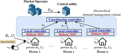
Based on a high-level view, the proposed scheme can be described under three sections: (a) the application of the LR method to obtain a fully-automated hierarchical DR framework in which household local controllers communicate with a coordinating controller at the central utility; (b) implementing a robust MPC scheme at each local controller to attain design requirements of the end-user while accounting for internal and external sources of uncertainties at household level; (c) establishing the coordination among local controllers via a coordinating controller in order to achieve desired tracking of the load set-point signal.

3.1. Alternative formulation of the problem based on the LR method

A careful look at the centralised robust MPC problem (10a(10a) $\underset{\mathbf{u}(k+j)}{min}\underset{\mathbf{w}(k+j)}{max}\sum _{j=0}^{N-1}{\mathit{\ell }}_j(\mathbf{u}(k+j\mid k))$(10a) ) reveals that the original problem cannot be decomposed into a set of sub-problems due to the coupling of individual subsystems via the power balance constraint (10f). However, in the absence of (10f), the stage cost ${\ell }_j(\mathbf{x}(k\mid k),\mathbf{u}(k+j\mid k))$ of the original problem can be expressed as a sum of individual stage costs given by: (11) ${\mathit{\ell }}_j(\mathbf{u}(k+j\mid k))=\sum _{i=1}^n{\ell }_{i,j}(u_i(k+j\mid k)),j\in {\mathbb{Z}}_{[0,N-1]}$(11) where ${\ell }_{i,j}(x_i(k+j\mid k),u_i(k+j\mid k)):{\mathbb{R}}^2\to \mathbb{R}$ represents the stage cost of the sub-problem at ith household for $(k+j)$th sampling instant.

Proposition 3.1

The stage cost in (11(11) ${\mathit{\ell }}_j(\mathbf{u}(k+j\mid k))=\sum _{i=1}^n{\ell }_{i,j}(u_i(k+j\mid k)),j\in {\mathbb{Z}}_{[0,N-1]}$(11) ) is convex.

Proof.

The stage cost ${\mathit{\ell }}_j(\mathbf{u}(k+j\mid k))$ is a quadratic function of $\mathit{u}$, hence the convexity is preserved.

Since the stage cost ${\ell }_{i,j}(\mathbf{u}(k+j\mid k))$ is quadratic and convex with respect to $\mathbf{u}(k)$ and the coupling of subsystems is only through a single complicating constraint, the LR method (Conejo et al., 2006) is applied by relaxing the constraint given by (10f).

Without loss of generality, let us consider the certainty equivalent problem of (10a(10a) $\underset{\mathbf{u}(k+j)}{min}\underset{\mathbf{w}(k+j)}{max}\sum _{j=0}^{N-1}{\mathit{\ell }}_j(\mathbf{u}(k+j\mid k))$(10a) ), in other words, the centralised control problem with no uncertainties in the system.

If partial duality over the constraint (10f) of the original problem (10a(10a) $\underset{\mathbf{u}(k+j)}{min}\underset{\mathbf{w}(k+j)}{max}\sum _{j=0}^{N-1}{\mathit{\ell }}_j(\mathbf{u}(k+j\mid k))$(10a) ) is carried out, the Lagrangian function ($\mathcal{L}$) can be derived as: (12) $\begin{array}{rl}& \mathcal{L}(u_i(k+j\mid k),\lambda (k+j))\\ & =\sum _{j=0}^{N-1}\sum _{i=1}^n[{\ell }_{i,j}(u_i(k+j\mid k))]\\ & +\sum _{j=0}^{N-1}[\lambda (k+j)(\sum _{i=1}^n{u}_i(k+j\mid k)-P_{\mathrm{ref}}(k+j))]\end{array}$(12) where $\lambda (k+j)\in {\mathbb{R}}^{}$ is the Lagrangian multiplier associated with the complicating input constraint given by (10f) of the original problem at $(k+j)$th sampling instant.

Simplifying the expression for the Lagrangian function in (12(12) $\begin{array}{rl}& \mathcal{L}(u_i(k+j\mid k),\lambda (k+j))\\ & =\sum _{j=0}^{N-1}\sum _{i=1}^n[{\ell }_{i,j}(u_i(k+j\mid k))]\\ & +\sum _{j=0}^{N-1}[\lambda (k+j)(\sum _{i=1}^n{u}_i(k+j\mid k)-P_{\mathrm{ref}}(k+j))]\end{array}$(12) ) yields, (13) $\begin{array}{rl}& \mathcal{L}(u_i(k+j\mid k),\lambda (k+j))\\ & =\sum _{i=1}^n[\sum _{j=0}^{N-1}{\ell }_{i,j}(u_i(k+j\mid k))+\lambda (k+j)u_i(k+j\mid k)]\\ & -\sum _{j=0}^{N-1}[\lambda (k+j)\cdot P_{\mathrm{ref}}(k+j)]\end{array}$(13) Evaluating the dual function $\mathit{\varphi }(\lambda )$ for given values of Lagrangian multipliers $\lambda (k+j)=\hat{\lambda }(k+j)$ for $j\in {\mathbb{Z}}_{[0,N-1]}$ gives, (14) $\begin{array}{rl}& \mathit{\varphi }(\hat{\lambda }(k+j))\\ & =\underset{u_i(k+j)}{min}\sum _{i=1}^n[\sum _{j=0}^{N-1}{\ell }_{i,j}(u_i(k+j\mid k))\\ & +\hat{\lambda }(k+j)u_i(k+j\mid k)\phantom{\sum _{j=0}^{N-1}}]-\sum _{j=0}^{N-1}\hat{\lambda }(k+j)P_{\mathrm{ref}}(k+j)\\ & \text{subject to (10b)}-\text{(10e)};j\in {\mathbb{Z}}_{[0,N-1]},i=1,\dots ,n.\end{array}$(14) By dropping the constant term $\sum _{j=0}^{N-1}[\hat{\lambda }(k+j)\cdot P_{\mathrm{ref}}(k+j)]$, the dual function in (14(14) $\begin{array}{rl}& \mathit{\varphi }(\hat{\lambda }(k+j))\\ & =\underset{u_i(k+j)}{min}\sum _{i=1}^n[\sum _{j=0}^{N-1}{\ell }_{i,j}(u_i(k+j\mid k))\\ & +\hat{\lambda }(k+j)u_i(k+j\mid k)\phantom{\sum _{j=0}^{N-1}}]-\sum _{j=0}^{N-1}\hat{\lambda }(k+j)P_{\mathrm{ref}}(k+j)\\ & \text{subject to (10b)}-\text{(10e)};j\in {\mathbb{Z}}_{[0,N-1]},i=1,\dots ,n.\end{array}$(14) ) can be reduced to: (15) $\begin{array}{rl}& \mathit{\psi }(\hat{\lambda }(k+j))\\ & =\underset{u_i(k+j)}{min}\sum _{i=1}^n[\sum _{j=0}^{N-1}{\ell }_{i,j}(u_i(k+j\mid k))\\ & +\hat{\lambda }(k+j)u_i(k+j\mid k)\phantom{\sum _{j=0}^{N-1}}]\\ & \text{subject to (10b)}-\text{(10e)};j\in {\mathbb{Z}}_{[0,N-1]},i=1,\dots ,n.\end{array}$(15) The reduced form of the dual function in (15(15) $\begin{array}{rl}& \mathit{\psi }(\hat{\lambda }(k+j))\\ & =\underset{u_i(k+j)}{min}\sum _{i=1}^n[\sum _{j=0}^{N-1}{\ell }_{i,j}(u_i(k+j\mid k))\\ & +\hat{\lambda }(k+j)u_i(k+j\mid k)\phantom{\sum _{j=0}^{N-1}}]\\ & \text{subject to (10b)}-\text{(10e)};j\in {\mathbb{Z}}_{[0,N-1]},i=1,\dots ,n.\end{array}$(15) ) can be decomposed into a set of sub-problems as follows: (16) $\begin{array}{rl}& \underset{u_i(k+j)}{min}\sum _{j=0}^{N-1}{\ell }_{i,j}(u_i(k+j\mid k))+\hat{\lambda }(k+j)u_i(k+j\mid k)\\ & \text{subject to: constraints for the}i\text{th subsystem derived}\\ & \text{from (10b)}-\text{(10e)};\\ & j\in {\mathbb{Z}}_{[0,N-1]}\end{array}$(16) A local agent responsible for each subsystem given by $i\in \{1,\dots ,n\}$ can solve problem (16(16) $\begin{array}{rl}& \underset{u_i(k+j)}{min}\sum _{j=0}^{N-1}{\ell }_{i,j}(u_i(k+j\mid k))+\hat{\lambda }(k+j)u_i(k+j\mid k)\\ & \text{subject to: constraints for the}i\text{th subsystem derived}\\ & \text{from (10b)}-\text{(10e)};\\ & j\in {\mathbb{Z}}_{[0,N-1]}\end{array}$(16) ) independently and to evaluate the dual problem.

Lemma 3.2

Lagrangian bounding principle Conejo et al., 2006

For any set of Lagrangian multipliers $\mathit{\lambda }=\{\lambda (k),\dots ,\lambda (k+N-1)\}\in {\mathbb{R}}^N$, the value of $\mathit{\varphi }(\mathit{\lambda })$ of the Lagrangian dual function is a lower bound of the optimal objective function value of the original problem.

Consequently, the Lagrangian dual problem gives the best lower bound of the optimal objective function of the original problem. This can be mathematically expressed as: (17) ${\mathit{\varphi }}^{\ast }=\underset{\lambda }{\mathrm{maximise}}\mathit{\varphi }(\mathit{\lambda })$(17)

Lemma 3.3

Strong duality Conejo et al., 2006

If the primal problem is convex, the optimal solution ${\mathit{\varphi }}^{\ast }$ of the Lagrangian dual problem coincides with the optimal solution to the primal problem.

Let optimal values of Lagrangian multipliers of the dual problem (17(17) ${\mathit{\varphi }}^{\ast }=\underset{\lambda }{\mathrm{maximise}}\mathit{\varphi }(\mathit{\lambda })$(17) ) be ${\mathit{\lambda }}^{\ast }=\{{\lambda }^{\ast }(k),\dots ,{\lambda }^{\ast }(k+N-1)\}$; from strong duality, $u_i^{\ast }(k+j)$ for $i\in \{1,\dots ,n\}$ for $j\in {\mathbb{Z}}_{[0,N-1]}$ gives the optimal values of the primal problem.

Proposition 3.4

The dual function $\varphi (\lambda )$ is concave.

Proof.

The Lagrangian function $\mathcal{L}(u,\lambda )$ in (12(12) $\begin{array}{rl}& \mathcal{L}(u_i(k+j\mid k),\lambda (k+j))\\ & =\sum _{j=0}^{N-1}\sum _{i=1}^n[{\ell }_{i,j}(u_i(k+j\mid k))]\\ & +\sum _{j=0}^{N-1}[\lambda (k+j)(\sum _{i=1}^n{u}_i(k+j\mid k)-P_{\mathrm{ref}}(k+j))]\end{array}$(12) ) is affine in λ. Hence, the Lagrangian dual function $\varphi (\lambda )=\underset{u}{inf}\mathcal{L}(u,\lambda )$ is concave because it is the pointwise infimum of a set of affine functions.

From duality theory (Boyd & Vandenberghe, 2004), the dual function can be maximised via an iterative steepest-ascent procedure. Following this, the sub-gradient method (Conejo et al., 2006) is employed to update the Lagrangian multiplier at each iteration. Considering νth iteration, the multiplier update is given by: (18) $\begin{array}{rl}{\lambda }^{(\nu +1)}(k+j)& ={\lambda }^{(\nu )}(k+j)+\frac{1}{a+\mathrm{b\nu }}\cdot \frac{s^{(\nu )}(k+j)}{\Vert s^{(\nu )}(k+j){\Vert }_2},\\ & j\in {\mathbb{Z}}_{[0,N-1]}\end{array}$(18) where a, b are scalar constants which need to determined and $s^{(\nu )}(k+j)$ is the sub-gradient of the dual function in νth iteration at $(k+j)$th sampling instant which is given by: (19) $s^{(\nu )}(k+j)=\sum _{i=1}^n{u}_i^{(\nu )}(k+j\mid k)-P_{\mathrm{ref}}(k+j),j\in {\mathbb{Z}}_{[0,N-1]}$(19) In summary, the LR-based formulation suggests that control actions can be implemented hierarchically with local controllers at each household implementing (16(16) $\begin{array}{rl}& \underset{u_i(k+j)}{min}\sum _{j=0}^{N-1}{\ell }_{i,j}(u_i(k+j\mid k))+\hat{\lambda }(k+j)u_i(k+j\mid k)\\ & \text{subject to: constraints for the}i\text{th subsystem derived}\\ & \text{from (10b)}-\text{(10e)};\\ & j\in {\mathbb{Z}}_{[0,N-1]}\end{array}$(16) ) and a coordinating controller at the central utility implementing (18(18) $\begin{array}{rl}{\lambda }^{(\nu +1)}(k+j)& ={\lambda }^{(\nu )}(k+j)+\frac{1}{a+\mathrm{b\nu }}\cdot \frac{s^{(\nu )}(k+j)}{\Vert s^{(\nu )}(k+j){\Vert }_2},\\ & j\in {\mathbb{Z}}_{[0,N-1]}\end{array}$(18) ) and (19(19) $s^{(\nu )}(k+j)=\sum _{i=1}^n{u}_i^{(\nu )}(k+j\mid k)-P_{\mathrm{ref}}(k+j),j\in {\mathbb{Z}}_{[0,N-1]}$(19) ).

3.2. Local controller

Aligned with the LR-based formulation introduced in Section 3.1, each household local controller implements robust MPC (Bemporad & Morari, 1999) to manage the consumption of the household air conditioner to provide real-time DR while accounting for household thermal model mismatches and outdoor temperature forecast errors. The control problem for the ith local controller at $(\nu +1)$th iteration can be expressed as: (20a) $\begin{array}{rl}& \underset{u_i^{(\nu +1)}(k+j)}{min}\underset{w_i(k+j)}{max}\sum _{j=0}^{N-1}[{\ell }_{i,j}(u_i(k+j\mid k))\\ & +{\lambda }^{(\nu )}(k+j)\cdot u_i(k+j\mid k)]\end{array}$(20a) subject to: (20b) $\begin{array}{rl}& {\mathbf{x}}_i(k)={\mathcal{A}}_i{\mathbf{x}}_i(k\mid k)+{\mathcal{B}}_i{\mathbf{u}}_i(k)+{\mathcal{D}}_i{\mathbf{v}}_i(k)+{\mathcal{G}}_i{\mathbf{w}}_i(k)\end{array}$(20b) (20c) $\begin{array}{rl}& {\mathbf{y}}_i(k)={\mathcal{E}}_i{\mathbf{x}}_i(k)\end{array}$(20c) (20d) $\begin{array}{rl}& {\underset{\_}{y}}_i\le y_i(k+j\mid k)\le {\overline{y}}_i,j\in {\mathbb{Z}}_{[0,N-1]},\mathrm{\forall }{w}_i\in {\mathcal{W}}_i\end{array}$(20d) (20e) $\begin{array}{rl}& 0\le u_i(k+j\mid k)\le {\overline{u}}_i,j\in {\mathbb{Z}}_{[0,N-1]},\mathrm{\forall }{w}_i\in {\mathcal{W}}_i\end{array}$(20e) (20f) $\begin{array}{rl}& w_i(k+j\mid k)\in {\mathcal{W}}_i\end{array}$(20f) where ${\mathcal{A}}_i$, ${\mathcal{B}}_i$, ${\mathcal{D}}_i$, ${\mathcal{G}}_i$ and ${\mathcal{E}}_i$ are the matrices derived for the ith subsystem based on the compact form of the aggregate state-space model in (8(8a) $\begin{array}{rl}\mathbf{x}(k)& =\mathcal{A}\mathbf{x}(k\mid k)+\mathcal{B}\mathbf{u}(k)+\mathcal{D}\mathbf{v}(k)+\mathcal{G}\mathbf{w}(k)\end{array}$(8a) ).

Additionally, the quadratic stage cost ${\ell }_{i,j}$ for the ith subsystem is derived from (9(9) ${\mathit{\ell }}_j(\mathbf{u}(k+j\mid k))={\mathbf{u}}^{\mathrm{T}}(k+j\mid k)\cdot \mathbf{u}(k+j\mid k)j\in {\mathbb{Z}}_{[0,N-1]}$(9) ) and expressed as: (21) ${\ell }_{i,j}(u_i(k+j))=u_i^2(k+j\mid k),j\in {\mathbb{Z}}_{[0,N-1]}$(21) The overall cost function in (20a(20a) $\begin{array}{rl}& \underset{u_i^{(\nu +1)}(k+j)}{min}\underset{w_i(k+j)}{max}\sum _{j=0}^{N-1}[{\ell }_{i,j}(u_i(k+j\mid k))\\ & +{\lambda }^{(\nu )}(k+j)\cdot u_i(k+j\mid k)]\end{array}$(20a) ) is derived from (16(16) $\begin{array}{rl}& \underset{u_i(k+j)}{min}\sum _{j=0}^{N-1}{\ell }_{i,j}(u_i(k+j\mid k))+\hat{\lambda }(k+j)u_i(k+j\mid k)\\ & \text{subject to: constraints for the}i\text{th subsystem derived}\\ & \text{from (10b)}-\text{(10e)};\\ & j\in {\mathbb{Z}}_{[0,N-1]}\end{array}$(16) ). The state and output are given by (20b(20b) $\begin{array}{rl}& {\mathbf{x}}_i(k)={\mathcal{A}}_i{\mathbf{x}}_i(k\mid k)+{\mathcal{B}}_i{\mathbf{u}}_i(k)+{\mathcal{D}}_i{\mathbf{v}}_i(k)+{\mathcal{G}}_i{\mathbf{w}}_i(k)\end{array}$(20b) ) and (20c(20c) $\begin{array}{rl}& {\mathbf{y}}_i(k)={\mathcal{E}}_i{\mathbf{x}}_i(k)\end{array}$(20c) ) respectively. The constraints on outputs are given by (20d(20d) $\begin{array}{rl}& {\underset{\_}{y}}_i\le y_i(k+j\mid k)\le {\overline{y}}_i,j\in {\mathbb{Z}}_{[0,N-1]},\mathrm{\forall }{w}_i\in {\mathcal{W}}_i\end{array}$(20d) ) and the constraints on inputs are given by (20e(20e) $\begin{array}{rl}& 0\le u_i(k+j\mid k)\le {\overline{u}}_i,j\in {\mathbb{Z}}_{[0,N-1]},\mathrm{\forall }{w}_i\in {\mathcal{W}}_i\end{array}$(20e) ). Furthermore, (20f(20f) $\begin{array}{rl}& w_i(k+j\mid k)\in {\mathcal{W}}_i\end{array}$(20f) ) represents the set to which the uncertainty in ith subsystem belongs to. In addition to that, the box-constrained uncertainty set ${\mathcal{W}}_i\subset {\mathbb{R}}^{}$ is described by, (22) ${\mathcal{W}}_i=\{w_i:\Vert w_i{\Vert }_{\mathrm{\infty }}\le w_0\}$(22) where $w_0$ is the worst-case uncertainty associated with the thermal model of ith house. The procedure to estimate $w_0$ based on the deviation of thermal parameters $R_i$, $C_i$ from their nominal values and the maximum forecast error of outdoor temperature is given in Appendix A. In this manner, ith local controller solves (20(20a) $\begin{array}{rl}& \underset{u_i^{(\nu +1)}(k+j)}{min}\underset{w_i(k+j)}{max}\sum _{j=0}^{N-1}[{\ell }_{i,j}(u_i(k+j\mid k))\\ & +{\lambda }^{(\nu )}(k+j)\cdot u_i(k+j\mid k)]\end{array}$(20a) ) at each iteration to determine the optimal control sequence $\{u_i(k),\dots ,u_i(k+N-1)\}$ while accounting for all possible uncertainties described by $w_i(k+j)$.

3.3. Coordinating controller

In this hierarchical control architecture, the coordinating controller acts as the mediating agent implemented at the central utility. While each local controller selfishly minimises input energy, the coordinating controller attempts to reach consensus, i.e. tracking the load set-point reference signal, by updating the Lagrangian multiplier at each iteration. Aligned with the decomposition based on the LR method described in Section 3.1 and the MPC scheme described in Section 3.2, the multiplier update at the coordinating controller at $(\nu +1)$th iteration at $(k+j)$th sampling instant can be expressed as: (23) $\begin{array}{rl}{\lambda }^{(\nu +1)}(k+j)& ={\lambda }^{(\nu )}(k+j)+\frac{1}{a+\mathrm{b\nu }}\cdot \frac{s^{(\nu )}(k+j)}{\Vert s^{(\nu )}(k+j){\Vert }_2},\\ & j\in {\mathbb{Z}}_{[0,N-1]}\end{array}$(23)

3.4. Convergence of the LR-based algorithm

Since the dual function is non-differentiable and concave as described in Section 3.1, the maximum is found via a steepest-ascent procedure. Aligned with that, the sub-gradient method is utilised to update the Lagrangian multiplier at each iteration. Therefore, the convergence criteria is set to be: (24) $\frac{\Vert {\lambda }^{(\nu +1)}(k+j)-{\lambda }^{(\nu -1)}(k+j)\Vert }{\Vert {\lambda }^{(\nu )}(k+j)\Vert }\le ϵ,j\in {\mathbb{Z}}_{[0,N-1]}$(24) where ϵ is the minimum tolerance for convergence which is a scalar. In other words, at a particular sampling instant, the LR-based robust MPC scheme executes until the convergence criteria in (24(24) $\frac{\Vert {\lambda }^{(\nu +1)}(k+j)-{\lambda }^{(\nu -1)}(k+j)\Vert }{\Vert {\lambda }^{(\nu )}(k+j)\Vert }\le ϵ,j\in {\mathbb{Z}}_{[0,N-1]}$(24) ) is met. Thereafter, the execution of the algorithm at the next sampling begins.

In addition to a minimum accuracy criteria determined by (24(24) $\frac{\Vert {\lambda }^{(\nu +1)}(k+j)-{\lambda }^{(\nu -1)}(k+j)\Vert }{\Vert {\lambda }^{(\nu )}(k+j)\Vert }\le ϵ,j\in {\mathbb{Z}}_{[0,N-1]}$(24) ), a maximum iteration criteria, maxiter, is also utilised to accelerate the computation of the overall algorithm. In other words, if the gradient is unable to reach the accuracy margin, the algorithm will terminate after maxiter iterations at a certain sampling instant, without further optimising to reach convergence.

The overall implementation of the real-time DR scheme is given in Algorithm 1. For instance, at νth iteration of kth sampling instant, each local controller solves (20(20a) $\begin{array}{rl}& \underset{u_i^{(\nu +1)}(k+j)}{min}\underset{w_i(k+j)}{max}\sum _{j=0}^{N-1}[{\ell }_{i,j}(u_i(k+j\mid k))\\ & +{\lambda }^{(\nu )}(k+j)\cdot u_i(k+j\mid k)]\end{array}$(20a) ) in parallel with Lagrangian multipliers from the previous step to determine the optimal control sequence $u_i^{(\nu )}(k+j)$ for $j\in {\mathbb{Z}}_{[0,N-1]}$ and sends information to the coordinating controller. With information from all the local controllers, the coordinating controller updates the Lagrangian multiplier for the $(\nu +1)$th iteration as in (23(23) $\begin{array}{rl}{\lambda }^{(\nu +1)}(k+j)& ={\lambda }^{(\nu )}(k+j)+\frac{1}{a+\mathrm{b\nu }}\cdot \frac{s^{(\nu )}(k+j)}{\Vert s^{(\nu )}(k+j){\Vert }_2},\\ & j\in {\mathbb{Z}}_{[0,N-1]}\end{array}$(23) ) and scatters among all the local controllers. With the updated Lagrangian multiplier, local controllers solve (20(20a) $\begin{array}{rl}& \underset{u_i^{(\nu +1)}(k+j)}{min}\underset{w_i(k+j)}{max}\sum _{j=0}^{N-1}[{\ell }_{i,j}(u_i(k+j\mid k))\\ & +{\lambda }^{(\nu )}(k+j)\cdot u_i(k+j\mid k)]\end{array}$(20a) ) back again to determine the optimal control sequence for the next iteration. Likewise, this back-and-forth optimal decision making and updating the Lagrangian multiplier processes repeat until the convergence criteria in (24(24) $\frac{\Vert {\lambda }^{(\nu +1)}(k+j)-{\lambda }^{(\nu -1)}(k+j)\Vert }{\Vert {\lambda }^{(\nu )}(k+j)\Vert }\le ϵ,j\in {\mathbb{Z}}_{[0,N-1]}$(24) ) is met. Let us assume that convergence criteria is met at ${\nu }^{\ast }$th iteration at kth sampling instant, then, each local controller assigns the first input of the optimal control sequence at the final iteration, i.e. $u_i^{({\nu }^{\ast })}(k)$, as the power consumption set-point for its own household air conditioner. After that, each local controller updates the state of the system based on output indoor temperature measurements $y_i(k)$ to determine the optimal control sequence for the next step. Likewise, this algorithm is repeated at each sampling instant until the DR event finishes.

It should be noted that a systematic coordination scheme between local controllers the coordinating controller is required for the proposed scheme to deliver desired outcomes in a realistic setting. In this regard, it is assumed that smart meter driven two-way communication infrastructure exists between local controllers at end-users and the coordinating controller at the central utility. Moreover, the latency associated with the communication link is assumed to be negligible with respect to the sampling period of 5-mins and the link possesses sufficient network bandwidth for reliable data transfer. The smart metering interface at end customers can be physically or virtually connected to the coordinating controller interface via a wired link such as copper, optical fiber, or a wireless link such as microwave (Kabalci, 2016). In addition to that, existing communication standards for DR such as OpenADR Alliance (n.d.) can be incorporated to ensure a reliable, secure and smooth automation.

Remark 3.1

In the proposed hierarchical control scheme, each household only needs to share information on R, C thermal parameters with the local controller in its own premises. Even if the parameters shared by each customer are inaccurate, the robust MPC implementation at the local controller effectively accounts for model parameter mismatches – only the nominal range of thermal parameters are required – in determining optimal power consumption set-points for household air conditioners. Moreover, compared to the central utility accessing real-time indoor temperature measurements, each local controller having access to household indoor temperatures under the full-state feedback implementation (20c(20c) $\begin{array}{rl}& {\mathbf{y}}_i(k)={\mathcal{E}}_i{\mathbf{x}}_i(k)\end{array}$(20c) ) is often realistic under the proposed hierarchical implementation. In addition to that, the power consumption set-point assigned to an air conditioner at a certain sampling instant, let's say k, which is $u_i^{({\nu }^{\ast })}(k)$, is only known to the ith local controller. By all means, it is guaranteed that end-user data privacy is preserved under limited data requirements between the aggregator and the local controller.

Remark 3.2

Unlike the centralised robust MPC implementation in (10(10a) $\underset{\mathbf{u}(k+j)}{min}\underset{\mathbf{w}(k+j)}{max}\sum _{j=0}^{N-1}{\mathit{\ell }}_j(\mathbf{u}(k+j\mid k))$(10a) ), the hierarchical implementation with household local controllers optimising their own design objectives significantly reduces the computational burden of the coordinating controller. To elaborate this further, consider a scenario where $n_h$ houses are under the central utility and an MPC scheme with a prediction horizon of $N_{\mathrm{pred}}$ is to be implemented to provide real-time demand management services. For the centralised robust MPC scheme, the robust counterpart should be determined based on uncertainty polytope having $(2^{N_{\mathrm{pred}}}{)}^{n_h}$ vertices (Scokaert & Mayne, 1998). Conversely, under the proposed hierarchical control scheme, a local controller at each household only needs to determine the robust counterpart based on a polytope with $2^{N_{\mathrm{pred}}}$ vertices which is also independent of $n_h$. Hence, it can be claimed that unlike the former approach which is intractable, the latter is computationally attractive and therefore scalable.

Remark 3.3

Different from the existing open-loop control implementation where the population of air-conditioners are assigned identical set-points irrespective of their operating states (Energex, 2022), household local controllers in the proposed implementation effectively take account of thermal comfort limits and while meeting end-user objectives. Furthermore, cost-effective implementation of household local controllers can be achieved by embedding them as an additional control feature in existing home energy management schemes (Energex, 2021).

4. Results

In order to validate the proposed control approach, it is considered that on a particular day, the central utility receives a signal $P_{\mathrm{ref}}$ from the market operator that should be tracked for a duration of $\mathcal{T}=2$ hrs. The nominal outdoor temperature profile is obtained from School of Earth & Environmental Sciences, The University of Queensland (n.d.) and the percentage error in forecasting outdoor temperature is obtained from Bureau of Meteorology (BoM), Australia (n.d.). To construct the reference signal, first, scheduled demand and generation data from the Australian Energy Market Operator (AEMO, n.d.) is obtained. Thereafter, a normalised reference signal is generated by comparing generation and demand data. In the next step, the baseline consumption for the control period is estimated for the scenario where all the air conditioners operate at their set-point temperature. Thereafter, similar to Liu and Shi (2016a), the actual reference signal is generated by assuming a regulation capacity of $15\mathrm{\%}$ from the baseline consumption. For the heterogeneous population of air conditioners, $P_{\mathrm{rated}}=\mathcal{U}(2.5,3.5)$ kW; $R=\mathcal{U}(1.5,2.5{)}^{\circ }\mathrm{C}/\mathrm{kW}$ with its nominal value at ${2.0}^{\circ }\mathrm{C}/\mathrm{kW}$; $C=\mathcal{U}(1.5,2.5)\mathrm{kWh}/{}^{\circ }\mathrm{C}$ with its nominal value at ${2.0}^{\circ }\mathrm{kWh}/{}^{\circ }\mathrm{C}$ and $\eta =2.5$ are obtained from Mathieu et al. (2013). The thermal limits are $\underset{\_}{y}={22}^{\circ }\mathrm{C}$ and $\overline{y}={24}^{\circ }\mathrm{C}$ considering the operation of air-conditioners aligned with Australian Institute of Refrigeration Air Conditioning and Heating (AIRAH, n.d.) guidelines Australian Institute of Refrigeration Air Conditioning & Heating (AIRAH). Prior to the event, it is assumed that all the air conditioners operate at their preferred thermal set-point which is ${23}^{\circ }\mathrm{C}$. For the local controller implementation described by (20(20a) $\begin{array}{rl}& \underset{u_i^{(\nu +1)}(k+j)}{min}\underset{w_i(k+j)}{max}\sum _{j=0}^{N-1}[{\ell }_{i,j}(u_i(k+j\mid k))\\ & +{\lambda }^{(\nu )}(k+j)\cdot u_i(k+j\mid k)]\end{array}$(20a) ), the upper limit of control input (${\overline{u}}_i\mathrm{\forall }i$) is obtained from $P_{\mathrm{rated}}$, the lower and upper limits of output (corresponds to end-user thermal comfort limits) are $\underset{\_}{y}={22}^{\circ }\mathrm{C}$ and $\overline{y}={24}^{\circ }\mathrm{C}$. Furthermore, ${\mathcal{A}}_i$, ${\mathcal{B}}_i$, ${\mathcal{D}}_i$, ${\mathcal{G}}_i$ and ${\mathcal{E}}_i$ for all i are derived from the aggregate state-space model described by (8(8a) $\begin{array}{rl}\mathbf{x}(k)& =\mathcal{A}\mathbf{x}(k\mid k)+\mathcal{B}\mathbf{u}(k)+\mathcal{D}\mathbf{v}(k)+\mathcal{G}\mathbf{w}(k)\end{array}$(8a) ). The uncertainty associated with the thermal model ($w_i\mathrm{\forall }i$) follows the derivation in Appendix A. For the robust distributed MPC implementation, the sampling interval Δ is considered to be 5-mins to align with the operation of Australian Energy Market Operator (AEMO, n.d.). The prediction horizon of the overall MPC scheme is N = 15-mins. For the LR method, the parameters of the multiplier update in (18(18) $\begin{array}{rl}{\lambda }^{(\nu +1)}(k+j)& ={\lambda }^{(\nu )}(k+j)+\frac{1}{a+\mathrm{b\nu }}\cdot \frac{s^{(\nu )}(k+j)}{\Vert s^{(\nu )}(k+j){\Vert }_2},\\ & j\in {\mathbb{Z}}_{[0,N-1]}\end{array}$(18) ) are a = 1 and b = 0.1 (Conejo et al., 2006). The termination criteria $ϵ=0.01$ and maxiter is chosen to be 50. The algorithms are written in MATLAB with YALMIP toolbox (Löfberg, 2004) and Gurobi 8.0.1 (Gurobi Optimization, L. L. C., 2021) is used as the solver. The simulations are performed on a computing facility equipped with Intel(R) Xeon(R) CPU E5-2680 v3 2.50 GHz and 64 GB RAM.

4.1. Tracking performance

The performance of the control scheme is studied for different aggregation sizes n = 100, 250, 500 under the following scenarios:

• scenario A: certainty-equivalent scenario

• scenario B: $w_i\sim \mathcal{U}(-w_0,w_0)\mathrm{\forall }i$ with $w_0={0.10}^{\circ }\mathrm{C}$

• scenario C: $w_i\sim \mathcal{U}(-w_0,w_0)\mathrm{\forall }i$ with $w_0={0.15}^{\circ }\mathrm{C}$

• scenario D: $w_i\sim \mathcal{U}(-w_0,w_0)\mathrm{\forall }i$ with $w_0={0.20}^{\circ }\mathrm{C}$

To further explain this, scenario A corresponds to the case where perfect information on thermal model parameters and outdoor temperature forecasts are available. On the other hand, under scenario B, the worst-case additive disturbance ($w_0$) for each air-conditioning subsystem estimated as in Appendix A with the percentage forecast error of outdoor temperature and thermal parameter mismatches is calculated to be ${0.10}^{\circ }\mathrm{C}$. Subsequently, for simulation purposes, the uncertainty associated with the thermal model for each house at each sampling instant is obtained from a uniform distribution bounded by $(-w_0,w_0)$.

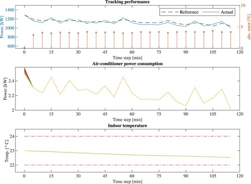
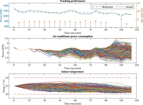
Figure 2 illustrates the aggregate tracking performance and the variation of power consumption and indoor temperature for n = 500 household air-conditioners while providing under scenario A. As can be seen from the figure, accurate load set-point tracking can be achieved with a maximum absolute error of approximately 5% under the certainty-equivalent scenario. Furthermore, the power consumption of air-conditioners follows an identical profile in the range 2.0–2.5 kW. A further inspection of the power consumption profile yields that it is a scaled version of the aggregate profile. This can be understood by the equal allocation of power set-points for air-conditioners under the LR method in the absence of uncertainties. Since the initial indoor temperature is assumed to be ${23}^{\circ }\mathrm{C}$, outdoor temperature profile is identical, and R, C thermal parameters are assumed to be at their nominal values ${2.0}^{\circ }\mathrm{C}/\mathrm{kW}$ and $2.0\mathrm{kWh}/{}^{\circ }\mathrm{C}$ for all air-conditioners under scenario A, the indoor temperature profile is identical and remains within thermal comfort limits $[22,24{]}^{\circ }\mathrm{C}$.

Figure 2. Scenario A: certainty-equivalent scenario for n = 500.

Moving on to the scenarios where uncertainties are present in the system, Figure 3 provides information on the performance of the overall hierarchical control scheme under scenario B. It can be seen that the proposed scheme is able to deliver precise load set-point tracking performance with a maximum tracking error of $<5$% under $w_0={0.10}^{\circ }\mathrm{C}$. Furthermore, it is observed that the power consumption profile remains identical up to around 40-mins. Thereafter, the power consumption significantly deviates from the identical equipartition profile for most of the air-conditioners. Since most air-conditioners tend to hit their thermal limits after 45-mins, especially the lower thermal bound, the power consumption profile drifts from the identical profile to avoid thermal comfort violations. This results in a wide range of power consumption variation, 1.0–2.5 kW, compared to scenario A. Nonetheless, the indoor temperature is maintained within thermal comfort limits.

Figure 3. Scenario B: $w_0={0.10}^{\circ }\mathrm{C}$ for n = 500.

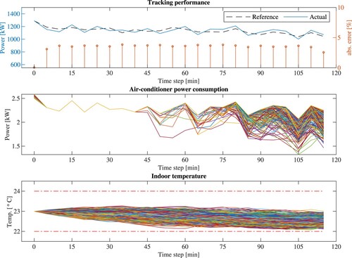
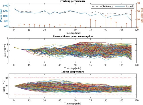
Figure 4 represents the aggregate tracking performance, the variation of power consumption and indoor temperature for n = 500 household air-conditioners under scenario C. As can be seen from the figure, when the degree of uncertainties is further increased to $w_0={0.15}^{\circ }\mathrm{C}$, the aggregate tracking error tends to go beyond 5% limit towards the end of the DR event. Moreover, compared to scenario B, the air-conditioners maintain an identical profile only up to 15-mins and drifts from the nominal profile as indoor temperature tends to reach comfort limits. This concludes that the rate at which indoor temperature tends to hit thermal limits increases with the degree of uncertainty associated with the overall system. Consequently, the range of operation of air-conditioners further expands to 1.0–3.5 kW compared to scenario B. However, indoor temperature is maintained within $[22,24{]}^{\circ }\mathrm{C}$ even in the presence of worst-case uncertainties at $w_0={0.15}^{\circ }\mathrm{C}$.

Figure 4. Scenario C: $w_0={0.15}^{\circ }\mathrm{C}$ for n = 500.

When the degree of uncertainties is further increased to $w_0={0.20}^{\circ }\mathrm{C}$ under scenario D as shown in Figure 5, the tracking performance degrades and results in approximately 20% tracking error towards the end of the DR event. Furthermore, equipartition allocation is only observed for about 10-mins and thereupon, the power consumption profile significantly varies from the nominal profile. For certain durations, (60–90 mins), some air-conditioners operate at their rated consumption to mitigate temperature comfort violations. Consequently, the power consumption varies in a much wider range (0–4 kW) compared to other scenarios. Not only that, unlike the other scenarios where indoor temperature tries to reach the lower bound which is ${22}^{\circ }\mathrm{C}$, under scenario D, it is observed that for some air-conditioners indoor temperature reaches the lower thermal limit whereas for other air-conditioners, the indoor temperature tends to reach the upper thermal limit which is ${24}^{\circ }\mathrm{C}$. However, even with $w_0={0.20}^{\circ }\mathrm{C}$, the proposed hierarchical control scheme is able to maintain thermal comfort for end-users at the expense of reduced tracking performance.

Figure 5. Scenario D: $w_0={0.20}^{\circ }\mathrm{C}$ for n = 500.

4.2. Scalability of the approach

The computational performance of the hierarchical DR scheme under uncertainties is compared against its counterpart–certainty equivalent scenario. A summary of the results in terms of total computation time (in minutes) for different aggregation sizes with and without uncertainties are given in Table 2.

Table 2. Comparison of the total execution time under different scenarios.

		Total execution time in the presence of uncertainties (min)
Aggregation size (n)	Total execution time under the certainty-equivalent scenario (min)	$w_0={0.10}^{\circ }\mathrm{C}$	$w_0={0.15}^{\circ }\mathrm{C}$	$w_0={0.20}^{\circ }\mathrm{C}$	$w_0={0.25}^{\circ }\mathrm{C}$
100	26.85	26.02	26.74	20.71	inf.
250	60.66	61.17	57.28	59.95	inf.
500	108.0	112.2	107.1	110.5	inf.

Note: – simulations are carried out on a computing facility equipped with Intel(R) Xeon(R) CPU E5-2680 v3 2.50 GHz and 64 GB RAM memory.– the local controller algorithm (20(20a) $\begin{array}{rl}& \underset{u_i^{(\nu +1)}(k+j)}{min}\underset{w_i(k+j)}{max}\sum _{j=0}^{N-1}[{\ell }_{i,j}(u_i(k+j\mid k))\\ & +{\lambda }^{(\nu )}(k+j)\cdot u_i(k+j\mid k)]\end{array}$(20a) ) is executed in parallel.

It can be seen from the data in Table 2 that the proposed robust control scheme is able to deliver DR within the allocated time, i.e. $\mathcal{T}=2-\mathrm{hrs}=120-\mathrm{mins}$, for all the scenarios in the presence of uncertainties under an aggregation size of n = 500. Hence, it can be claimed that the proposed hierarchical DR scheme is computationally scalable compared to the centralised robust implementation in (10a(10a) $\underset{\mathbf{u}(k+j)}{min}\underset{\mathbf{w}(k+j)}{max}\sum _{j=0}^{N-1}{\mathit{\ell }}_j(\mathbf{u}(k+j\mid k))$(10a) ). Furthermore, the robust MPC implementation at household local controllers is able to achieve the same level of computational performance as a perfect controller which represents the certainty-equivalent scenario.

A further inspection of the results in Table 2 suggests that the proposed approach leads to an infeasible problem if the worst-case uncertainty ($w_0$) associated with each subsystem is ${0.25}^{\circ }\mathrm{C}$. To put it differently, the local controller fails to find an optimal solution to problem (20a(20a) $\begin{array}{rl}& \underset{u_i^{(\nu +1)}(k+j)}{min}\underset{w_i(k+j)}{max}\sum _{j=0}^{N-1}[{\ell }_{i,j}(u_i(k+j\mid k))\\ & +{\lambda }^{(\nu )}(k+j)\cdot u_i(k+j\mid k)]\end{array}$(20a) ) for $w_0={0.25}^{\circ }\mathrm{C}$ without violating constraints on thermal comfort defined by (20d(20d) $\begin{array}{rl}& {\underset{\_}{y}}_i\le y_i(k+j\mid k)\le {\overline{y}}_i,j\in {\mathbb{Z}}_{[0,N-1]},\mathrm{\forall }{w}_i\in {\mathcal{W}}_i\end{array}$(20d) ). This is intuitive as the control law for open-loop robust MPC is inapplicable due to infeasibility when unknown disturbances affect the process (Scokaert & Mayne, 1998). Nevertheless, a performance bound for the overall DR scheme under uncertainties can be obtained based on estimated worst-case uncertainties ($w_0$) by adopting the proposed method.

4.3. Convergence of the LR scheme

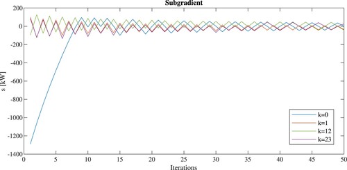
The convergence behaviour of the Lagrangian multiplier (λ) and the subgradient (s) in Section 3.4 for different time steps (k = 0, 1, 12, 23) under n = 500 with $w_0={0.10}^{\circ }\mathrm{C}$ is shown in Figures 6 and 7 respectively. Looking at plots, it is apparent that the Lagrangian multiplier (λ) and the sub-gradient (s) exhibit oscillatory convergence as expected in the subgradient method (Conejo et al., 2006). As can be seen from Figure 6, λ is initialised at 0 for the first iteration at k = 0. Thereupon, after reaching maxiter iterations as discussed in Section 3.4, a ‘warm-start’ approach is adopted. To explain this, the value of λ for the 50th iteration at k = 0 is set to be the value of λ for the first iteration at k = 1. This 'warm-start' technique is utilised to speed up the convergence of the overall algorithm at a certain time step. Moreover, this will result in low oscillations in λ in succeeding time steps as observed in Figure 6. Similarly, the subgradient varies significantly at the first iteration of k = 0 when λ is initialised at 0. Afterwards, s tends to converge in an oscillatory manner in the range $\pm 40$ kW until maxiter criteria is met.

Figure 6. The convergence of λ at different time steps under $w_0={0.10}^{\circ }\mathrm{C}$ for n = 500.

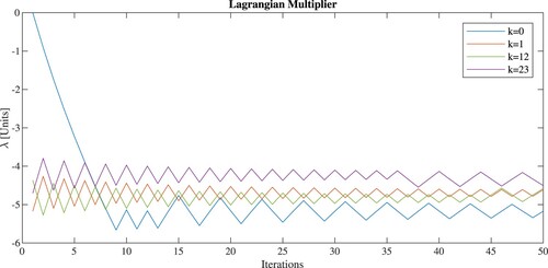
Figure 7. The convergence of s at different time steps under $w_0={0.10}^{\circ }\mathrm{C}$ for n = 500.

It is worth mentioning that the tracking performance depends on maxiter convergence criteria. The tracking performance can be further improved especially under scenario A if maxiter is set at a value greater than 50. However, this will increase the computational time of the overall algorithm. To summarise, the proposed hierarchical control scheme converges within an acceptable range with the adoption of double termination criteria.

5. Conclusions and future work

This paper develops a robust hierarchical control scheme for residential TCLs to provide DR in grid services. First, a centralised formulation of the control problem at the central utility is considered. Afterwards, an equivalent decomposable structure with a local controller at each household and a coordinating controller at the central utility is derived by relaxing the power balance constraint via the LR method. To enhance the resiliency of the proposed DR scheme against uncertainties in a real-world setting, a robust MPC implementation is adopted at household local controllers that account for model parameter mismatches and outdoor temperature forecast errors. Furthermore, data privacy of end-users is preserved as they are only required to share household-specific information with the local controllers in their own premises. Using inverter-type air-conditioners as the controllable load, the simulation studies are validated on a real reference signal obtained from the Australian Energy Market Operator. Some of the key findings of the study are:

• As the degree of uncertainty increases, the DR tracking performance degrades. Nevertheless, the proposed robust hierarchical control scheme is able to provide desired DR with an upper bound of error at $\sim 20\mathrm{\%}$ under $w_0={0.20}^{\circ }\mathrm{C}$ degree of uncertainties while regulating indoor temperature within $[22,24{]}^{\circ }\mathrm{C}$.

• Beyond $w_0={0.20}^{\circ }\mathrm{C}$, the robust implementation is infeasible as the local controllers fail to find an optimal solution without violating thermal comfort limits for end-users. Hence, the proposed approach can be utilised to determine a performance bound of uncertainties in a realistic setting.

• The same level of computational performance of a perfect controller, i.e. a control implementation without any uncertainties in the system, can be achieved by the proposed hierarchical robust MPC scheme with the adoption of double termination criteria. Hence, the overall approach is scalable.

In future work, it would be interesting to assess the effect of latency and imperfections in the communication infrastructure on the performance of the proposed hierarchical DR scheme.

Disclosure statement

The authors declare that they have no known competing financial interests or personal relationships that could have appeared to influence the work reported in this paper.

Additional information

Funding

This work was supported by the Centre for Energy Data Innovation (CEDI), The University of Queensland, under the Advance Queensland grant (grant no: AQPTP01216-17RD1).

Appendix. Derivation of the worst-case uncertainty limits

Consider the thermal model of the ith air conditioning subsystem (without explicitly considering uncertainties as a stochastic disturbance), (A1) $x_i(k+1)=A_i{x}_i(k)+B_i{u}_i(k)+D_i{v}_i(k)$(A1) where the notation follows the same as in (1a(1a) $\begin{array}{rl}{x}_i(k+1)& =A_i{x}_i(k)+B_i{u}_i(k)+D_i{v}_i(k)+w_i(k)\end{array}$(1a) ).

Let $R_i$ and $C_i$ information be imperfect, then their actual values can be expressed as: $\begin{array}{rl}{R}_i& ={\tilde{R}}_i+\mathrm{\Delta }{R}_i\\ C_i& ={\tilde{C}}_i+\mathrm{\Delta }{C}_i\end{array}$where ${\tilde{R}}_i$ and ${\tilde{C}}_i$ are the nominal values of $R_i$ and $C_i$ parameters, $\mathrm{\Delta }{R}_i$ and $\mathrm{\Delta }{C}_i$ are the deviations of $R_i$ and $C_i$ from their nominal values respectively. Hence, $A_i$ term in (1a(1a) $\begin{array}{rl}{x}_i(k+1)& =A_i{x}_i(k)+B_i{u}_i(k)+D_i{v}_i(k)+w_i(k)\end{array}$(1a) ) can be expressed as: (A2) $\begin{array}{rl}{A}_i& =\exp \left(\frac{-h}{({\tilde{R}}_i+\mathrm{\Delta }{R}_i)\cdot ({\tilde{C}}_i+\mathrm{\Delta }{C}_i)}\right)\end{array}$(A2) (A3) $\begin{array}{rl}{A}_i& =\exp \left(\frac{-h}{({\tilde{R}}_i\cdot {\tilde{C}}_i+{\tilde{R}}_i\cdot \mathrm{\Delta }{C}_i+\mathrm{\Delta }{C}_i\cdot {\tilde{R}}_i+\mathrm{\Delta }{R}_i)\cdot \mathrm{\Delta }{R}_i}\right)\end{array}$(A3) Using Taylor series expansion to linearise (A3(A3) $\begin{array}{rl}{A}_i& =\exp \left(\frac{-h}{({\tilde{R}}_i\cdot {\tilde{C}}_i+{\tilde{R}}_i\cdot \mathrm{\Delta }{C}_i+\mathrm{\Delta }{C}_i\cdot {\tilde{R}}_i+\mathrm{\Delta }{R}_i)\cdot \mathrm{\Delta }{R}_i}\right)\end{array}$(A3) ), the value of $A_i$ can be approximated by, (A4) $A_i={\tilde{A}}_i+\mathrm{\Delta }{A}_i$(A4) where ${\tilde{A}}_i=e^{-h/({\tilde{R}}_i\cdot {\tilde{C}}_i)}$ is the nominal value of $A_i$ and $\mathrm{\Delta }{A}_i$ is the deviation from the nominal value of $A_i$ due to model parameter mismatches.

Similarly, $B_i$ and $D_i$ can be represented as, (A5) $\begin{array}{rl}{B}_i& ={\tilde{B}}_i+\mathrm{\Delta }{B}_i\end{array}$(A5) (A6) $\begin{array}{rl}{D}_i& ={\tilde{D}}_i+\mathrm{\Delta }{D}_i\end{array}$(A6) Let the nominal forecast of outdoor temperature at time k be ${\tilde{v}}_i(k)$ and the error in predicting outdoor temperature be $\mathrm{\Delta }{v}_i(k)$. Thereafter, substituting (A4(A4) $A_i={\tilde{A}}_i+\mathrm{\Delta }{A}_i$(A4) ), (A5(A5) $\begin{array}{rl}{B}_i& ={\tilde{B}}_i+\mathrm{\Delta }{B}_i\end{array}$(A5) ) and (A6(A6) $\begin{array}{rl}{D}_i& ={\tilde{D}}_i+\mathrm{\Delta }{D}_i\end{array}$(A6) ), and the actual value of $v(k)$ in (A1(A1) $x_i(k+1)=A_i{x}_i(k)+B_i{u}_i(k)+D_i{v}_i(k)$(A1) ) yields, (A7) $\begin{array}{rl}{x}_i(k+1)& =({\tilde{A}}_i+\mathrm{\Delta }{A}_i)\cdot x_i(k)+({\tilde{B}}_i+\mathrm{\Delta }{B}_i)\cdot u_i(k)\\ & +({\tilde{D}}_i+\mathrm{\Delta }{D}_i)\cdot ({\tilde{v}}_i(k)+\mathrm{\Delta }{v}_i(k))\end{array}$(A7) Separating the certain terms and representing the uncertain terms with an additive stochastic term ($w_i$) can derived as: (A8) $w_i(k)=\mathrm{\Delta }{A}_i\cdot x_i(k)+\mathrm{\Delta }{B}_i\cdot u_i(k)+\mathrm{\Delta }{D}_i\cdot {\tilde{v}}_i(k)+\mathrm{\Delta }{D}_i\cdot \mathrm{\Delta }{v}_i(k)$(A8) Hence (A7(A7) $\begin{array}{rl}{x}_i(k+1)& =({\tilde{A}}_i+\mathrm{\Delta }{A}_i)\cdot x_i(k)+({\tilde{B}}_i+\mathrm{\Delta }{B}_i)\cdot u_i(k)\\ & +({\tilde{D}}_i+\mathrm{\Delta }{D}_i)\cdot ({\tilde{v}}_i(k)+\mathrm{\Delta }{v}_i(k))\end{array}$(A7) ) can be rewritten as, (A9) $x_i(k+1)={\tilde{A}}_i\cdot x_i(k)+{\tilde{B}}_i\cdot u_i(k)+{\tilde{D}}_i\cdot {\tilde{v}}_i(k)+w_i(k)$(A9) For brevity and ease of notation, $(\tilde{\cdot })$ notation is dropped and (A9(A9) $x_i(k+1)={\tilde{A}}_i\cdot x_i(k)+{\tilde{B}}_i\cdot u_i(k)+{\tilde{D}}_i\cdot {\tilde{v}}_i(k)+w_i(k)$(A9) ) is re-written as, (A10) $x_i(k+1)=A_i\cdot x_i(k)+B_i\cdot u_i(k)+D_i\cdot v_i(k)+w_i(k)$(A10)

References

- Australian Energy Market Operator (AEMO) (n.d.). National electricity market (NEM) data dashboard. https://aemo.com.au/en/energy-systems/electricity/national-electricity-market-nem/data-nem/data-dashboard-nem.
- Australian Institute of Refrigeration Air Conditioning and Heating (AIRAH) (n.d.). DA09 air conditioning load estimation and psychrometrics. Retrieved January 26, 2023, from https://www.airah.org.au/DA_manuals/DA_Manuals/Manuals.aspx.
- Australian Renewable Energy Agency (2019). Demand response RERT trial year 1 report. Retrieved December 23, 2019, from https://arena.gov.au/assets/2019/03/demand-response-rert-trial-year-1-report.pdf.
- Bashash, S., & Fathy, H. K. (2013, July). Modeling and control of aggregate air conditioning loads for robust renewable power management. IEEE Transactions on Control Systems Technology, 21(4), 1318–1327. https://doi.org/10.1109/TCST.2012.2204261
- Bemporad, A., & Morari, M. (1999). Robust model predictive control: A survey. In A. Garulli & A. Tesi (Eds.), Robustness in identification and control (pp. 207–226). Springer London.
- Ben-Tal, A., El Ghaoui, L., & Nemirovski, A. S. (2009). Robust optimization. Princeton University Press.
- Bertsimas, D., & Sim, M. (2004). The price of robustness. Operations Research, 52(1), 35–53. https://doi.org/10.1287/opre.1030.0065
- Boyd, S. P., & Vandenberghe, L. (2004). Convex optimization. Cambridge University Press.
- Bureau of Meteorology (BoM), Australia (n.d.). Bureau forecast accuracy. Retrieved April 27, 2020, from http://www.bom.gov.au/inside/forecast-accuracy.shtml.
- Burger, E. M., & Moura, S. J. (2017, May). Generation following with thermostatically controlled loads via alternating direction method of multipliers sharing algorithm. Electric Power Systems Research, 146, 141–160. https://doi.org/10.1016/j.epsr.2016.12.001
- Callaway, D. S. (2009). Tapping the energy storage potential in electric loads to deliver load following and regulation, with application to wind energy. Energy Conversion and Management, 50(5), 1389–1400. https://doi.org/10.1016/j.enconman.2008.12.012
- Callaway, D. S., & Hiskens, I. A. (2011, January). Achieving controllability of electric loads. Proceedings of the IEEE, 99(1), 184–199. https://doi.org/10.1109/JPROC.2010.2081652
- Camponogara, E., Jia, D., Krogh, B. H., & Talukdar, S. (2002). Distributed model predictive control. IEEE Control Systems Magazine, 22(1), 44–52. https://doi.org/10.1109/37.980246
- Chen, C., Wang, J., & Kishore, S. (2014). A distributed direct load control approach for large-scale residential demand response. IEEE Transactions on Power Systems, 29(5), 2219–2228. https://doi.org/10.1109/TPWRS.2014.2307474
- Conejo, A., Castillo, E., Minguez, R., & Garcia-Bertrand, R. (2006). Decomposition in nonlinear programming. In Decomposition techniques in mathematical programming: Engineering and science applications (pp. 187–242). Springer Berlin Heidelberg. https://doi.org/10.1007/3-540-27686-6_5
- Department of Environment and Energy Australia (2019). Consultation paper: ‘Smart’ demand response capabilities for selected appliances. Retrieved December 23, 2019, from https://www.energyrating.gov.au/document/consultation-paper-smart-demand-response-capabilities-selected-appliances.
- Diekerhof, M., Peterssen, F., & Monti, A. (2018). Hierarchical distributed robust optimization for demand response services. IEEE Transactions on Smart Grid, 9(6), 6018–6029. https://doi.org/10.1109/TSG.2017.2701821
- Energex (2021). Home energy management systems. https://www.energex.com.au/home/control-your-energy/smarter-energy/home-energy-management-systems.
- Energex (2022). PeakSmart events. https://www.energex.com.au/home/control-your-energy/managing-electricity-demand/peak-demand/peaksmart-events.
- Erdinc, O., Tascikaraoglu, A., Paterakis, N. G., & Catalao, J. P. S. (2019, February). Novel incentive mechanism for end-users enrolled in DLC-based demand response programs within stochastic planning context. IEEE Transactions on Industrial Electronics, 66(2), 1476–1487. https://doi.org/10.1109/TIE.2018.2811403
- Goulart, P. J., Kerrigan, E. C., & Maciejowski, J. M. (2006). Optimization over state feedback policies for robust control with constraints. Automatica, 42(4), 523–533. https://doi.org/10.1016/j.automatica.2005.08.023
- Gurobi Optimization, L. L. C. (2021). Gurobi optimizer reference manual. http://www.gurobi.com.
- Halvgaard, R., Vandenberghe, L., Poulsen, N. K., Madsen, H., & J. B. Jørgensen (2016). Distributed model predictive control for smart energy systems. IEEE Transactions on Smart Grid, 7(3), 1675–1682. https://doi.org/10.1109/TSG.2016.2526077
- Hu, Q., Li, F., Fang, X., & Bai, L. (2018, January). A framework of residential demand aggregation with financial incentives. IEEE Transactions on Smart Grid, 9(1), 497–505. https://doi.org/10.1109/TSG.2016.2631083
- Hui, H., Ding, Y., & Zheng, M. (2019). Equivalent modeling of inverter air conditioners for providing frequency regulation service. IEEE Transactions on Industrial Electronics, 66(2), 1413–1423. https://doi.org/10.1109/TIE.2018.2831192
- Kabalci, Y. (2016). A survey on smart metering and smart grid communication. Renewable and Sustainable Energy Reviews, 57, 302–318. https://doi.org/10.1016/j.rser.2015.12.114
- Katipamula, S., & Lu, N. (2006). Evaluation of residential HVAC control strategies for demand response programs. ASHRAE Transactions, 112(1), 535–546.
- Larsen, G. K. H., van Foreest, N. D., & Scherpen, J. M. A. (2013, June). Distributed control of the power supply-demand balance. IEEE Transactions on Smart Grid, 4(2), 828–836. https://doi.org/10.1109/TSG.2013.2242907
- Liu, M., & Shi, Y. (2014). Distributed model predictive control of thermostatically controlled appliances for providing balancing service. In 53rd IEEE conference on decision and control (pp. 4850–4855). IEEE.
- Liu, M., & Shi, Y. (2016a). Model predictive control for thermostatically controlled appliances providing balancing service. IEEE Transactions on Control Systems Technology, 24(6), 2082–2093. https://doi.org/10.1109/TCST.2016.2535400
- Liu, M., & Shi, Y. (2016b). Model predictive control of aggregated heterogeneous second-order thermostatically controlled loads for ancillary services. IEEE Transactions on Power Systems, 31(3), 1963–1971. https://doi.org/10.1109/TPWRS.2015.2457428
- Löfberg, J. (2004). YALMIP: A toolbox for modeling and optimization in MATLAB. In Proceedings of the IEEE international symposium on computer-aided control system design (pp. 284–289). IEEE. https://doi.org/10.1109/cacsd.2004.1393890
- Lork, C., Li, W. T., Qin, Y., Zhou, Y., Yuen, C., Tushar, W., & Saha, T. K. (2020). An uncertainty-aware deep reinforcement learning framework for residential air conditioning energy management. Applied Energy, 276, Article 115426. https://doi.org/10.1016/j.apenergy.2020.115426
- Lu, N. (2012). An evaluation of the HVAC load potential for providing load balancing service. IEEE Transactions on Smart Grid, 3(3), 1263–1270. https://doi.org/10.1109/TSG.2012.2183649
- Maasoumy, M., Razmara, M., Shahbakhti, M., & Vincentelli, A. S. (2014). Handling model uncertainty in model predictive control for energy efficient buildings. Energy and Buildings, 77, 377–392. https://doi.org/10.1016/j.enbuild.2014.03.057
- Mahdavi, N., & Braslavsky, J. H. (2020, September). Modelling and control of ensembles of variable-speed air conditioning loads for demand response. IEEE Transactions on Smart Grid, 11(5), 4249–4260. https://doi.org/10.1109/TSG.2020.2991835
- Mahdavi, N., Braslavsky, J. H., Seron, M. M., & West, S. R. (2017, November). Model predictive control of distributed air-conditioning loads to compensate fluctuations in solar power. IEEE Transactions on Smart Grid, 8(6), 3055–3065. https://doi.org/10.1109/TSG.2017.2717447
- Mathieu, J. L., Koch, S., & Callaway, D. S. (2013). State estimation and control of electric loads to manage real-time energy imbalance. IEEE Transactions on Power Systems, 28(1), 430–440. https://doi.org/10.1109/TPWRS.2012.2204074
- Molina, A., Gabaldon, A., Fuentes, J. A., & Alvarez, C. (2003). Implementation and assessment of physically based electrical load models: Application to direct load control residential programmes. IEE Proceedings-Generation, Transmission and Distribution, 150(1), 61–66. https://doi.org/10.1049/ip-gtd:20020750
- Molzahn, D. K., Dörfler, F., Sandberg, H., Low, S. H., Chakrabarti, S., Baldick, R., & Lavaei, J. (2017, November). A survey of distributed optimization and control algorithms for electric power systems. IEEE Transactions on Smart Grid, 8(6), 2941–2962. https://doi.org/10.1109/TSG.2017.2720471
- Oldewurtel, F., C. N. Jones, Parisio, A., & Morari, M. (2014, May). Stochastic model predictive control for building climate control. IEEE Transactions on Control Systems Technology, 22(3), 1198–1205. https://doi.org/10.1109/TCST.2013.2272178
- OpenADR Alliance (n.d.). OpenADR 2.0 demand response program implementation guide. Retrieved May 12, 2020, from https://www.openadr.org/assets/openadr_drprogramguide_v1.0.pdf.
- Palensky, P., & Dietrich, D. (2011, August). Demand side management: Demand response, intelligent energy systems, and smart loads. IEEE Transactions on Industrial Informatics, 7(3), 381–388. https://doi.org/10.1109/TII.2011.2158841
- Papadaskalopoulos, D., & Strbac, G. (2013, November). Decentralized participation of flexible demand in electricity markets–Part I: Market mechanism. IEEE Transactions on Power Systems, 28(4), 3658–3666. https://doi.org/10.1109/TPWRS.2013.2245686
- Pillitteri, V., & Brewer, T. (2014). Guidelines for smart grid cybersecurity (NIST Interagency/Internal Report (NISTIR)). National Institute of Standards and Technology, Gaithersburg, MD. https://doi.org/10.6028/NIST.IR.7628r1
- PJM (2022). Markets & operations. https://www.pjm.com/markets-and-operations.aspx.
- Scattolini, R. (2009). Architectures for distributed and hierarchical model predictive control–a review. Journal of Process Control, 19(5), 723–731. https://doi.org/10.1016/j.jprocont.2009.02.003
- School of Earth and Environmental Sciences, The University of Queensland (n.d.). UQ weatherstations. Retrieved August 20, 2020, from https://bit.ly/2PXuc2n.
- Scokaert, P. O. M., & Mayne, D. Q. (1998, August). Min-max feedback model predictive control for constrained linear systems. IEEE Transactions on Automatic Control, 43(8), 1136–1142. https://doi.org/10.1109/9.704989
- Thomas, E., Sharma, R., & Nazarathy, Y. (2019, March). Towards demand side management control using household specific Markovian models. Automatica, 101, 450–457. https://doi.org/10.1016/j.automatica.2018.11.057
- Tindemans, S. H., Trovato, V., & Strbac, G. (2015). Decentralized control of thermostatic loads for flexible demand response. IEEE Transactions on Control Systems Technology, 23(5), 1685–1700. https://doi.org/10.1109/TCST.2014.2381163.
- Vrettos, E., Oldewurtel, F., & Andersson, G. (2016). Robust energy-constrained frequency reserves from aggregations of commercial buildings. IEEE Transactions on Power Systems, 31(6), 4272–4285. https://doi.org/10.1109/TPWRS.2015.2511541
- Zhang, W., Lian, J., Chang, C. Y., & Kalsi, K. (2013, November). Aggregated modeling and control of air conditioning loads for demand response. IEEE Transactions on Power Systems, 28(4), 4655–4664. https://doi.org/10.1109/TPWRS.2013.2266121