Robustness improvement of optimal control in terms of RBFNN with empirical model reduction and transfer learning

Abstract

This paper proposes a method to compute solutions of optimal controls for dynamic systems in terms of radial basis function neural networks (RBFNN) with Gaussian neurons. The RBFNN is used to compute the value function from Hamilton–Jacobi–Bellman equation with the policy iteration. The concept of dominant system is introduced to create initial coefficients of the neural networks to stabilise unstable systems and guarantee the convergence of policy iteration. Model reduction and transfer learning techniques are introduced to improve robustness of RBFNN optimal control, and reduce computational time. Numerical and experimental results show that the resulting optimal control has excellent control performance in stabilisation and trajectory tracking, and much-improved robustness to disturbances and model uncertainties even when the system responses move to a domain of the state space that is larger than the domain where the neural networks are trained.

Keywords:

• Hamilton–Jacobi–Bellman equation
• radial basis function neural networks
• balanced truncation
• empirical gramian
• transfer learning

1. Introduction

Optimal controls are commonly determined with the help of the Hamilton–Jacobi–Bellman (HJB) equation. The HJB equation is a nonlinear partial differential equation for the value function of the optimal control problem. There have been many studies on the solution of the HJB equation in the mathematics and controls community. However, it remains a technical challenge to obtain analytical solutions of the HJB equation for nonlinear control problems. This paper presents a method to obtain approximate solutions of the HJB equation for nonlinear control systems. The method consists of radial basis function neural networks, reduced order modelling and transfer learning.

Crandall and Lions proposed the viscosity solution of the HJB equation in Crandall and Lions (1983), and found that the HJB equation exists non-smoothnesss solution. A sequential alternating least squares method to solve the high dimensional linear HJB equation was presented in Stefansson and Leong (2016). In addition to the numerical methods such as viscosity solution, finite difference and finite element, neural networks are other promising approaches that have garnered recent interest (Greif, 2017).

Neural networks have been extensively studied for solving partial differential equations (PDEs) (Han et al., 2018; Lagaris et al., 2000; Sirignano & Spiliopoulos, 2018). Neural networks with different activation functions have also been applied to the HJB equation (Munos et al., 1999; T. Nakamura-Zimmerer et al., 2021). The HJB equation with action constraints (Abu-Khalaf & Lewis, 2005; Yang et al., 2014) and fixed final time has been studied with the help of neural networks with polynomial neurons (Cheng et al., 2007a, 2007b). The least squares algorithm with a time-domain discounting factor and $\tanh (x)$ neuron was studied in Tassa and Erez (2007) to improve the smoothness and convergence of neural networks solutions. The activation function $\tanh (x)$ was also used to solve high dimensional HJB equations in T. Nakamura-Zimmerer et al. (2020). The rectified linear neurons were used to approximate the value function using a grid-free approach in Jiang et al. (2016). Effects of different types of neural networks for the solution of the Hamilton–Jacobi–Bellman equation are studied in Yang et al. (2014).

The radial basis neural networks (RBFNN) were used to compute the HJB solution along the response trajectory (D. Zhang et al., 2016). The normalised Gaussian networks were adopted to develop a reinforcement learning framework to obtain the global value function for continuous time systems while training the networks along different trajectories (Doya, 2000). The actor-critic reinforcement learning together with the RBFNN was also applied to obtain the optimal control for a discrete-time system (D. Zhang et al., 2016).

Recently, the interest in solving the HJB solution in high dimensional state space is growing (Darbon & Osher, 2016; Yegorov & Dower, 2021). A neural network with sigmoid activation function was proposed to compute the viability sets of nonlinear continuous systems in Djeridane and Lygeros (2006). The tanh activation function was considered to develop a causality-free neural network to solve high dimensional HJB equations including the co-state vector as part of the solution (T. Nakamura-Zimmerer et al., 2020; T. E. Nakamura-Zimmerer, 2022). Two neural networks architectures are introduced using minimum plus algebra to solve high dimensional optimal control problems with specified terminal cost using the min-pooling activation function in Darbon et al. (2021). Indeed, neural networks can obtain excellent approximations of the value function from the solution of the HJB equation leading to the optimal policy. Among all the neural networks structures and activation functions, the polynomial activation functions are adopted in most cases to solve the optimal control problems in reinforcement learning (Abu-Khalaf & Lewis, 2005; Cheng et al., 2007a, 2007b; Liu et al., 2014; Luo et al., 2014; Modares & Lewis, 2014; Modares et al., 2014; Yang et al., 2014).

While the solutions of the HJB equation have been extensively studied, fewer investigations have focussed on the performance of optimal controls obtained in terms of the RBFNN. This paper presents an approach based on radial basis function neural networks with Gaussian activation functions to solve the HJB equation for various optimal control problems and to demonstrate the robustness of the optimal controls with the model reduction and transfer learning technique in machine learning. This study addresses the robustness improvement of the optimal controls obtained with the RBFNN, model reduction and transfer learning.

There are many studies on the radial basis function neural networks. An adaptive extended Kalman filter (AEKF) was developed for estimating the weights, centres, and width of RBFNN (Medagam & Pourboghrat, 2009). It has been shown that the RBFNN with one hidden layer and the same smoothing factor in each kernel are broad enough for universal approximation (Park & Sandberg, 1991). The RBFNN have been extensively applied to regression and classification problems. An excellent review of this method can be found in Wu et al. (2012). The RBFNN have been shown to have advantage in terms of design, generality and tolerance to noises compared to other neural network structures (Yu et al., 2011). It has been found that RBFNN have an advantage over the conventional sigmoid neural networks (NN) owing to that the nth-dimensional gaussian function is well-established from probability theory, Kalman filtering, etc. (Lewis et al., 1998). An application of the RBFNN in control design can be found in W. Zhang et al. (2022) to approximate the error model in vibration suppression. The advantages of RBFNN motivate us to further explore the potential of the RBFNN method to solve the HJB equation for nonlinear control systems.

Many mechanical systems with multi-degrees of freedom are underactuated by design. The dynamics of these systems live in a relatively high dimensional state space. It turns out to be highly advantageous to discover a reduced order model of the system, in which the limited control efforts can be focussed to stabilise the system and achieve improved tracking performance. The reduced order model also decreases numerical complexities in solving the HJB equation for nonlinear control systems. For this reason, it is important to find a reduced order model of the system before applying the RBFNN method to solve the HJB equation.

The balanced truncation model reduction (BTMR) method is a popular algorithm in the controls community to reduce the dimension of the dynamic system with the help of principal component analysis and singular value decomposition of the Hankel matrix constructed with the controllability and observability gramians. It has received much attention from the research community in the past decades (Gugercin & Antoulas, 2004; Pernebo & Silverman, 1982). The balanced model reduction has been applied to control design for high dimensional systems with thousands of degrees of freedom (Huang & Kramer, 2020; Wu et al., 2020). The controllability and observability gramians for nonlinear control systems can be computed from input-output data, leading to the so-called empirical gramians (Himpe, 2018). In this paper, the BTMR algorithms with both model-based and empirical gramians are considered for improving the robustness of the RBFNN optimal control, so as to reduce the computation complexity.

Since the mathematical model of nonlinear control systems can never perfectly capture the dynamics of the real system, the RBFNN control based on the mathematical model may need fine tuning when it is applied to the physical system in an experimental setting. This is where the transfer learning technique of machine learning comes in. After certain experimental data is obtained, the neural networks can be partially retrained in order to further improve the performance of the control.

The objective of this paper is to propose an efficient, practical and useful RBFNN algorithm to solve the HJB equation in optimal control. We demonstrate the RBFNN optimal control design with a linear rotary pendulum system and several nonlinear systems. In particular, the robustness of the RBFNN optimal control is explored and reported in terms of stabilisation and tracking of the pendulum and other nonlinear systems. The traditional LQR control and the optimal control obtained with the polynomial neural networks are used as benchmarks to compare with the proposed RBFNN optimal control design.

The remainder of the paper is outlined as follows. Section 2 reviews the optimal control formulation in terms of the HJB equation. Section 3 presents the RBFNN method to solve the nonlinear HJB equation. Section 4 discusses the balanced truncation algorithm and the RBFNN optimal control with the reduced order model. Section 6 presents numerical simulations and experimental results of the RBFNN optimal control for linear systems. Section 7 presents numerical simulations of the RBFNN optimal control for the nonlinear systems. Section 8 concludes the paper.

2. The Hamilton–Jacobi–Bellman equation

Consider a nonlinear time-invariant dynamic system governed by the state equation (1) $\begin{array}{r}\dot{\mathbf{x}}(t)=\mathbf{f}(\mathbf{x})+\mathbf{g}(\mathbf{x})\mathbf{u},\mathbf{x}(t_0)={\mathbf{x}}_0,\end{array}$(1) where $t_0$ is the initial time, ${\mathbf{x}}_0$ is the initial state, $\mathbf{x}\in {\mathbb{R}}^{n\times 1}$, $\mathbf{u}\in {\mathbb{R}}^{m\times 1}$. $\mathbf{f}(\cdot )$ and $\mathbf{g}(\cdot )$ are nonlinear functions of their arguments. Define a target set at a terminal time t = T as (2) $\begin{array}{r}\varphi (\mathbf{x}(T),T)=0,\end{array}$(2) where $\varphi \in {\mathbb{R}}^{p\times 1}$. ϕ defines a set where the terminal state $\mathbf{x}(T)$ must settle at time T.

The optimal control problem amounts to finding a control $\mathbf{u}$ in an admissible set $U\subset {\mathbb{R}}^{m\times 1}$ that drives the system from the initial state ${\mathbf{x}}_0$ to the target set $\varphi (\mathbf{x}(T),T)$ such that the following performance index J is minimised while the state equation is satisfied. (3) $\begin{array}{r}J=\varphi (\mathbf{x}(T),T)+{\int }_{t_0}^T\mathcal{L}(\mathbf{x}(\tau ),\mathbf{u}(\tau ),\tau )\mathrm{d}\tau ,\end{array}$(3) where $\mathcal{L}(\mathbf{x}(t),\mathbf{u}(t),t)>0$ is called the Lagrange function.

Define a value function along the optimal trajectory based on the performance index as (4) $\begin{array}{rl}V({\mathbf{x}}^{\ast }(t),t)& =\varphi ({\mathbf{x}}^{\ast }(T),T)+{\int }_t^T\mathcal{L}({\mathbf{x}}^{\ast }(\tau ),{\mathbf{u}}^{\ast }(\tau ),\tau )\mathrm{d}\tau \\ & =\underset{\mathbf{u}}{min}[\varphi ({\mathbf{x}}^{\ast }(T),T)+{\int }_t^T\mathcal{L}({\mathbf{x}}^{\ast },\mathbf{u},\tau )\mathrm{d}\tau ].\end{array}$(4) By definition,the value function has the following properties (5) $\begin{array}{r}\begin{array}{rl}V({\mathbf{x}}^{\ast }(T),T)& =\varphi ({\mathbf{x}}^{\ast }(T),T),\\ V({\mathbf{x}}^{\ast }(t),t_0)& =J.\end{array}\end{array}$(5) Take the derivative of the value function with respect to time t based on the definition in Equation (4(4) $\begin{array}{rl}V({\mathbf{x}}^{\ast }(t),t)& =\varphi ({\mathbf{x}}^{\ast }(T),T)+{\int }_t^T\mathcal{L}({\mathbf{x}}^{\ast }(\tau ),{\mathbf{u}}^{\ast }(\tau ),\tau )\mathrm{d}\tau \\ & =\underset{\mathbf{u}}{min}[\varphi ({\mathbf{x}}^{\ast }(T),T)+{\int }_t^T\mathcal{L}({\mathbf{x}}^{\ast },\mathbf{u},\tau )\mathrm{d}\tau ].\end{array}$(4) ) (6) $\begin{array}{r}\frac{\mathrm{d}V({\mathbf{x}}^{\ast }(t),t)}{\mathrm{d}t}=-\mathcal{L}({\mathbf{x}}^{\ast }(t),{\mathbf{u}}^{\ast }(t),t).\end{array}$(6)

Remark 2.1

A remark on the role of the value function is in order. By definition, we have (7) $\begin{array}{r}V({\mathbf{x}}^{\ast }(t),t)\ge 0,\frac{\mathrm{d}V({\mathbf{x}}^{\ast }(t),t)}{\mathrm{d}t}\le 0.\end{array}$(7) Hence, $V({\mathbf{x}}^{\ast }(t),t)$ is a Lyapunov function. The existence of the Lyapunov function implies that the system under the optimal control ${\mathbf{u}}^{\ast }(t)$ is stable.

By treating $V({\mathbf{x}}^{\ast }(t),t)$ as a multi-variable function of the state and time, we can also apply the chain rule of differentiation along the optimal path to obtain the Hamilton–Jacobi–Bellman equation (HJB) as (8) $\begin{array}{rl}\frac{\mathrm{\partial }V({\mathbf{x}}^{\ast }(t),t)}{\mathrm{\partial }t}& =-\mathcal{L}({\mathbf{x}}^{\ast }(t),{\mathbf{u}}^{\ast }(t),t)\\ & -\frac{\mathrm{\partial }V({\mathbf{x}}^{\ast }(t),t{)}^T}{\mathrm{\partial }\mathbf{x}}(\mathbf{f}({\mathbf{x}}^{\ast }(t))+\mathbf{g}({\mathbf{x}}^{\ast }(t)){\mathbf{u}}^{\ast }(t))\\ & =-H({\mathbf{x}}^{\ast }(t),{\mathbf{u}}^{\ast }(t),\frac{\mathrm{\partial }V({\mathbf{x}}^{\ast }(t),t)}{\mathrm{\partial }\mathbf{x}},t)\\ & =-\underset{\mathbf{u}}{min}H({\mathbf{x}}^{\ast }(t),\mathbf{u}(t),\frac{\mathrm{\partial }V({\mathbf{x}}^{\ast }(t),t)}{\mathrm{\partial }\mathbf{x}},t),\end{array}$(8) where H is the Hamiltonian function defined as (9) $\begin{array}{rl}& H(\mathbf{x}(t),\mathbf{u}(t),\mathit{\lambda }(t),t)\\ & =\mathcal{L}(\mathbf{x}(t),\mathbf{u}(t),t)+{\mathit{\lambda }}^T(t)[\mathbf{f}(\mathbf{x}(t))+\mathbf{g}(\mathbf{x}(t))\mathbf{u}(t)],\end{array}$(9) and $\mathit{\lambda }(t)$ is a vector of Lagrange multipliers.

Equation (8(8) $\begin{array}{rl}\frac{\mathrm{\partial }V({\mathbf{x}}^{\ast }(t),t)}{\mathrm{\partial }t}& =-\mathcal{L}({\mathbf{x}}^{\ast }(t),{\mathbf{u}}^{\ast }(t),t)\\ & -\frac{\mathrm{\partial }V({\mathbf{x}}^{\ast }(t),t{)}^T}{\mathrm{\partial }\mathbf{x}}(\mathbf{f}({\mathbf{x}}^{\ast }(t))+\mathbf{g}({\mathbf{x}}^{\ast }(t)){\mathbf{u}}^{\ast }(t))\\ & =-H({\mathbf{x}}^{\ast }(t),{\mathbf{u}}^{\ast }(t),\frac{\mathrm{\partial }V({\mathbf{x}}^{\ast }(t),t)}{\mathrm{\partial }\mathbf{x}},t)\\ & =-\underset{\mathbf{u}}{min}H({\mathbf{x}}^{\ast }(t),\mathbf{u}(t),\frac{\mathrm{\partial }V({\mathbf{x}}^{\ast }(t),t)}{\mathrm{\partial }\mathbf{x}},t),\end{array}$(8) ) is a partial differential equation defined in the state space governing the value function. According to the definition of the value function, we have a terminal condition for the HJB equation as $V({\mathbf{x}}^{\ast }(T),T)=\varphi ({\mathbf{x}}^{\ast }(T),T)$. When there are constraints imposed on the states, boundary conditions can also be imposed to the HJB equation.

Consider a special case (10) $\begin{array}{r}\mathcal{L}(\mathbf{x},\mathbf{u})=\frac{1}{2}[{\mathbf{x}}^T(t)\mathbf{Qx}(t)+{\mathbf{u}}^T(t)\mathbf{Ru}(t)],\end{array}$(10) where $\mathbf{Q}$ is a semi-positive definite symmetrical matrix, and $\mathbf{R}$ is a positive definite symmetrical matrix. The optimal control for this case is expressed in terms of the value function. (11) $\begin{array}{r}{\mathbf{u}}^{\ast }(t)=-{\mathbf{R}}^{-1}{\mathbf{g}}^T({\mathbf{x}}^{\ast }(t))\frac{\mathrm{\partial }V({\mathbf{x}}^{\ast }(t),t)}{\mathrm{\partial }\mathbf{x}}.\end{array}$(11) When the system is nonlinear, it is difficult to obtain the function of $V({\mathbf{x}}^{\ast }(t),t)$ analytically. This study focuses on the RBFNN with Gaussian activation functions for obtaining the value function.

3. Neural networks solution of value function

In the following, we shall focus on the special time-invariant case when the terminal time $T\to \mathrm{\infty }$, the terminal cost $\varphi (\mathbf{x}(T),T)\to 0$, and the value function is only a function of the state, i.e. $V=V(\mathbf{x})$.

The value function can be expressed in terms of radial basis function neural networks with Gaussian activation functions, (12) $\begin{array}{rl}V(\mathbf{x},\mathbf{w}(k))& =\sum _{j=1}^{N_G}{w}_j(k)g(\mathbf{x},{\mathit{\mu }}_j,{\mathbf{\Sigma }}_j)+C\\ & \equiv {\mathbf{w}}^T(k)\mathbf{h}(\mathbf{x})+C\equiv {\mathbf{h}}^T(\mathbf{x})\mathbf{w}(k)+C,\end{array}$(12) where $N_G$ is the number of Gaussian functions $g(\mathbf{x},{\mathit{\mu }}_j,{\mathbf{\Sigma }}_j)$ and C is an arbitrary integration constant to guarantee the value function to be non-negative. (13) $\begin{array}{rl}g(\mathbf{x},{\mathit{\mu }}_j,{\mathbf{\Sigma }}_j)& =\prod _{i=1}^n\frac{1}{\sqrt{2\pi }{\sigma }_{j,i}}\exp [-\frac{1}{2{\sigma }_{j,i}^2}(x_i-{\mu }_{j,i}{)}^2]\end{array}$(13) (14) $\begin{array}{rl}& \equiv \prod _{i=1}^n{g}_j(x_i,{\mu }_{j,i},{\sigma }_{j,i})\end{array}$(14) The vectors and matrices in the above equations are defined as (15) $\begin{array}{rl}\mathbf{w}(k)& =[w_1(k),w_2(k),\dots ,w_{N_G}(k){]}^T\in {\mathbb{R}}^{N_G\times 1},\end{array}$(15) (16) $\begin{array}{rl}\mathbf{h}(\mathbf{x})& =[g(\mathbf{x},{\mathit{\mu }}_1,{\mathbf{\Sigma }}_1),g(\mathbf{x},{\mathit{\mu }}_2,{\mathbf{\Sigma }}_2),\dots ,\\ & \times g(\mathbf{x},{\mathit{\mu }}_{N_G},{\mathbf{\Sigma }}_{N_G}){]}^T\in {\mathbb{R}}^{N_G\times 1},\end{array}$(16) (17) $\begin{array}{rl}{\mathit{\mu }}_j& =[{\mu }_{j,i}]\in {\mathbb{R}}^{N_G\times n},\end{array}$(17) (18) $\begin{array}{rl}{\mathbf{\Sigma }}_j& =[{\sigma }_{j,i}]\in {\mathbb{R}}^{N_G\times n},\end{array}$(18) where k is the iteration index of the policy iteration algorithm introduced next. In general, the elements of the mean matrix ${\mathit{\mu }}_j$ and covariance matrix ${\mathbf{\Sigma }}_j$ can be trainable coefficients of the neural networks.

3.1. Implementation of RBFNN

In this study, the Gaussian functions are adopted as kernels to approximate an unknown function as is commonly done in statistics and mesh-free finite elements (J.-S. Chen et al., 2017; Silverman, 2018; Sun & Hsu, 1988) That is to say, a finite domain $\mathcal{D}$ of interest in the state space can be divided into grids and take the grid coordinates as the mean ${\mathit{\mu }}_j$. Furthermore, the covariance matrix ${\mathbf{\Sigma }}_j$ is taken to be diagonal and the same constant for all Gaussian functions. It is noteworthy that with these choices of the mean and covariance matrix, the RBFNN can indeed deliver sufficiently accurate solutions of nonlinear partial differential equations (Wang et al., 2022a, 2022b, 2023). It is shown in this paper that the optimal control for nonlinear dynamic systems can also be obtained in this manner, which allows us to focus on the issues in the control design.

Future efforts will treat both ${\mathit{\mu }}_j$ and ${\mathbf{\Sigma }}_j$ as trainable coefficients. The effect of varying means and standard deviations on the optimal control solution will be studied in a separate paper.

In the following discussions, we drop the symbol $\ast$ for optimal solutions for brevity.

3.2. Policy iteration (PI) algorithm

Recall the optimal control and consider the RBFNN solution of the value function in Equation (12(12) $\begin{array}{rl}V(\mathbf{x},\mathbf{w}(k))& =\sum _{j=1}^{N_G}{w}_j(k)g(\mathbf{x},{\mathit{\mu }}_j,{\mathbf{\Sigma }}_j)+C\\ & \equiv {\mathbf{w}}^T(k)\mathbf{h}(\mathbf{x})+C\equiv {\mathbf{h}}^T(\mathbf{x})\mathbf{w}(k)+C,\end{array}$(12) ). At the kth step of iterations, the control is given as (19) $\begin{array}{r}\mathbf{u}(\mathbf{x},k)=-{\mathbf{R}}^{-1}{\mathbf{g}}^T(\mathbf{x})\frac{\mathrm{\partial }V(\mathbf{x},\mathbf{w}(k))}{\mathrm{\partial }\mathbf{x}},\end{array}$(19) where $\mathbf{u}(\mathbf{x},k)$ and $V(\mathbf{x}(t),\mathbf{w}(k))$ denote the control and value function at the $k^{\mathrm{th}}$ step of iterations. $\mathbf{u}(\mathbf{x},k=0)$ is chosen to be a stabilising initial control. The value function is updated with the following equation, (20) $\begin{array}{r}\frac{\mathrm{\partial }{V}^T(\mathbf{x},\mathbf{w}(k+1))}{\mathrm{\partial }\mathbf{x}}(\mathbf{f}(\mathbf{x})+\mathbf{g}(\mathbf{x})\mathbf{u}(\mathbf{x},k))+\mathcal{L}(\mathbf{x},\mathbf{u}(\mathbf{x},k))=0.\end{array}$(20) According to Theorem 4 of reference Saridis and Lee (1979), the pair $\{\mathbf{u}(\mathbf{x},k),V(\mathbf{x},\mathbf{w}(k))\}$ determined by Equations (19(19) $\begin{array}{r}\mathbf{u}(\mathbf{x},k)=-{\mathbf{R}}^{-1}{\mathbf{g}}^T(\mathbf{x})\frac{\mathrm{\partial }V(\mathbf{x},\mathbf{w}(k))}{\mathrm{\partial }\mathbf{x}},\end{array}$(19) ) and (20(20) $\begin{array}{r}\frac{\mathrm{\partial }{V}^T(\mathbf{x},\mathbf{w}(k+1))}{\mathrm{\partial }\mathbf{x}}(\mathbf{f}(\mathbf{x})+\mathbf{g}(\mathbf{x})\mathbf{u}(\mathbf{x},k))+\mathcal{L}(\mathbf{x},\mathbf{u}(\mathbf{x},k))=0.\end{array}$(20) ) leads to a convergent sequence such that (21) $\begin{array}{r}\begin{array}{rl}V(\mathbf{x},\mathbf{w}(k))& \ge V(\mathbf{x},\mathbf{w}(k+1)),\\ \underset{k\to \mathrm{\infty }}{lim}V(\mathbf{x},\mathbf{w}(k))& =V^{\ast }(\mathbf{x}),\\ \underset{k\to \mathrm{\infty }}{lim}\mathbf{u}(\mathbf{x},k)& ={\mathbf{u}}^{\ast }(\mathbf{x})=-{\mathbf{R}}^{-1}{\mathbf{g}}^T(\mathbf{x})\frac{\mathrm{\partial }{V}^{\ast }(\mathbf{x})}{\mathrm{\partial }\mathbf{x}}.\end{array}\end{array}$(21) where $V^{\ast }(\mathbf{x})$ denotes the true optimal value function and ${\mathbf{u}}^{\ast }(\mathbf{x})$ is the true optimal control. Given a random value function and iteratively updating the new value function with the greedy policy is called value iteration or successive approximation (Saridis & Lee, 1979). Instead of updating the value function, the policy iteration is defined as iteratively updating the greedy policy to the optimal solution. Since the control $\mathbf{u}(\mathbf{x},k)$ and the value function are both iteratively updated during the calculation of the RBFNN, it is hard to distinguish the current approach as value iteration or policy iteration. In this case, it is treated as policy iteration. The proof of convergence of the similar algorithm for saturated controls was presented by Abu-Khalaf and Lewis (2005) and Meyn (2022). Many examples reported in the literature also confirm the convergence of the successive approximation algorithm (Tassa & Erez, 2007). We have found that the choice of an initial stabilising control policy ${\mathbf{u}}_0$ is important to put the PI algorithm on the right track to converge.

Next, the updating equation is presented in matrix form. Consider the expressions of Gaussian function in Equations (14(14) $\begin{array}{rl}& \equiv \prod _{i=1}^n{g}_j(x_i,{\mu }_{j,i},{\sigma }_{j,i})\end{array}$(14) )–(18(18) $\begin{array}{rl}{\mathbf{\Sigma }}_j& =[{\sigma }_{j,i}]\in {\mathbb{R}}^{N_G\times n},\end{array}$(18) ), the partial derivative is expressed as, (22) $\begin{array}{r}\begin{array}{rl}\frac{\mathrm{\partial }V(\mathbf{x},\mathbf{w}(k))}{\mathrm{\partial }{x}_i}& =\sum _{j=1}^{N_G}\frac{-(x_i-{\mu }_{j,i})}{{\sigma }_{j,i}^2}{w}_j(k)g_j(\mathbf{x},{\mu }_{\mathrm{ij}},{\sigma }_{\mathrm{ij}})\\ & \equiv \sum _{j=1}^{N_G}\frac{-(x_i-{\mu }_{j,i})}{{\sigma }_{j,i}^2}{w}_j(k)g(\mathbf{x},{\mathit{\mu }}_j,{\mathbf{\Sigma }}_j)\\ & \equiv \sum _{j=1}^{N_G}{d}_{i,j}(\mathbf{x})w_j(k),\end{array}\end{array}$(22) where (23) $\begin{array}{r}{d}_{i,j}(\mathbf{x})=\frac{-(x_i-{\mu }_{j,i})}{{\sigma }_{j,i}^2}g(\mathbf{x},{\mathit{\mu }}_j,{\mathbf{\Sigma }}_j).\end{array}$(23) Hence, the gradient of the value function is (24) $\begin{array}{r}\frac{\mathrm{\partial }V(\mathbf{x},\mathbf{w}(k))}{\mathrm{\partial }\mathbf{x}}=\mathbf{D}(\mathbf{x})\mathbf{w}(k)\in {\mathbb{R}}^{n\times 1},\end{array}$(24) where $\mathbf{D}=[d_{i,j}]\in {\mathbb{R}}^{n\times N_G}$ in Equation (23(23) $\begin{array}{r}{d}_{i,j}(\mathbf{x})=\frac{-(x_i-{\mu }_{j,i})}{{\sigma }_{j,i}^2}g(\mathbf{x},{\mathit{\mu }}_j,{\mathbf{\Sigma }}_j).\end{array}$(23) ). The control can now be written in the matrix form as (25) $\begin{array}{r}\mathbf{u}(\mathbf{x},k)=-{\mathbf{R}}^{-1}{\mathbf{g}}^T(\mathbf{x})\mathbf{D}(\mathbf{x})\mathbf{w}(k).\end{array}$(25) Equation (20(20) $\begin{array}{r}\frac{\mathrm{\partial }{V}^T(\mathbf{x},\mathbf{w}(k+1))}{\mathrm{\partial }\mathbf{x}}(\mathbf{f}(\mathbf{x})+\mathbf{g}(\mathbf{x})\mathbf{u}(\mathbf{x},k))+\mathcal{L}(\mathbf{x},\mathbf{u}(\mathbf{x},k))=0.\end{array}$(20) ) in terms of these matrices reads (26) $\begin{array}{r}{\mathbf{S}}^T(\mathbf{x})\mathbf{w}(k+1)+\mathcal{L}(\mathbf{x},\mathbf{u}(\mathbf{x},k))=0,\end{array}$(26) where $\mathbf{S}\in {\mathbb{R}}^{N_G\times 1}$ and (27) $\begin{array}{r}{\mathbf{S}}^T(\mathbf{x})=[\mathbf{f}(\mathbf{x})-\mathbf{g}(x){\mathbf{R}}^{-1}{\mathbf{g}}^T(\mathbf{x})\mathbf{D}(\mathbf{x})\mathbf{w}(k){]}^T\mathbf{D}(\mathbf{x}).\end{array}$(27) Define the error of the HJB equation due to the neural networks approximation as (28) $\begin{array}{r}e(\mathbf{x},\mathbf{w}(k+1))={\mathbf{S}}^T(\mathbf{x})\mathbf{w}(k+1)+\mathcal{L}(\mathbf{x},\mathbf{u}(\mathbf{x},k)).\end{array}$(28) An integrated squared error in the state space ${\mathbb{R}}^{n\times 1}$ is defined as (29) $\begin{array}{r}{J}_{\mathrm{HJB}}(\mathbf{w}(k+1))={\int }_{{\mathbb{R}}^{n\times 1}}\frac{1}{2}{e}^2(\mathbf{x},\mathbf{w}(k+1))d\mathbf{x}.\end{array}$(29)

3.3. Sampling method for integration

Computation of $J_{\mathrm{HJB}}(\mathbf{w}(k+1))$ involves integration in high dimensional space and can be intensive. Therefore, instead of integration in Equation (29(29) $\begin{array}{r}{J}_{\mathrm{HJB}}(\mathbf{w}(k+1))={\int }_{{\mathbb{R}}^{n\times 1}}\frac{1}{2}{e}^2(\mathbf{x},\mathbf{w}(k+1))d\mathbf{x}.\end{array}$(29) ), we can uniformly sample a large number of points ${\mathbf{x}}_s\in \mathcal{D}\subset {\mathbb{R}}^{n\times 1}$ to compute an approximate value of $J_{\mathrm{HJB}}(\mathbf{w}(k+1))$. A sampled value $J_s$ of $J_{\mathrm{HJB}}$ is obtained as (30) $\begin{array}{rl}{J}_s(\mathbf{w}(k+1))& =\frac{1}{2}\sum _{s=1}^{N_s}{e}^2({\mathbf{x}}_s,\mathbf{w}(k+1))\\ & =\frac{1}{2}\sum _{s=1}^{N_s}[{\mathbf{S}}^T({\mathbf{x}}_s)\mathbf{w}(k+1)+\mathcal{L}({\mathbf{x}}_s,\mathbf{u}({\mathbf{x}}_s,k)){]}^2\end{array}$(30) where $N_s$ is the number of sampled points ${\mathbf{x}}_s$ in the domain $\mathcal{D}$. Define the following matrix and vectors as (31) $\begin{array}{rl}{\mathbf{A}}_g(k)& ={\mathbf{A}}_g^T(k)=\sum _{s=1}^{N_s}\mathbf{S}{\mathbf{S}}^T({\mathbf{x}}_s)\in {\mathbb{R}}^{N_G\times N_G}\end{array}$(31) (32) $\begin{array}{rl}\mathbf{b}(k)& =\sum _{s=1}^{N_s}\mathcal{L}({\mathbf{x}}_s,\mathbf{u}({\mathbf{x}}_s,k))\mathbf{S}({\mathbf{x}}_s)\in {\mathbb{R}}^{N_G\times 1}\end{array}$(32) (33) $\begin{array}{rl}d(k)& =\frac{1}{2}\sum _{s=1}^{N_s}{\mathcal{L}}^2({\mathbf{x}}_s,\mathbf{u}({\mathbf{x}}_s,k))\in {\mathbb{R}}^1\end{array}$(33) Later in the examples, the domain $\mathcal{D}$ is referred to as the sampling region or training region.

The sampled performance index reads (34) $\begin{array}{rl}{J}_s(\mathbf{w}(k+1))& =\frac{1}{2}{\mathbf{w}}^T(k+1){\mathbf{A}}_g(k)\mathbf{w}(k+1)\\ & +{\mathbf{w}}^T(k+1)\mathbf{b}(k)+d(k).\end{array}$(34) The optimal coefficient vector at each iteration step can be obtained as (35) $\begin{array}{r}\mathbf{w}(k+1)=-{\mathbf{A}}_g^{-1}(k)\mathbf{b}(k)\end{array}$(35) assuming that the inverse of the matrix ${\mathbf{A}}_g^{-1}(k)$ exists. It has been found that when $N_s>N_G$, the inverse usually exists (Wang et al., 2022a, 2022b, 2023). The mean values and standard deviations of the Gaussian function are fixed in this paper. The state space is uniformly sampled along each dimension with a fixed grid size, and the standard deviation is set to be between four and five times the size of the fixed grid.

3.4. Dominant system

If the policy iteration algorithm starts with an initial estimate of the value function in terms of the RBFNN with randomly generated coefficients, the resulting control can push the system on to a track leading to instability for unstable systems. Hence, it is recommended to begin the policy iterations of an unstable system with a stabilising initial control, which will ensure system stability through the iteration process. We introduce the concept of dominant system to create the stabilising initial control. The dominant system is defined as an unstable linear system that has poles with larger positive real parts than that of the original system. A LQR control can be found to stabilise the dominant system and is used as the initial control to start the policy iteration. There are different ways to design the initial control, such as the supervised learning based control (Borovykh et al., 2022) and the unconstrained LQR control (Abu-Khalaf & Lewis, 2005). It should be noted that for stable systems, randomly generated initial coefficients $\mathbf{w}(1)$ for the RBFNN always make the policy iteration convergent.

4. Reduced order model

It has been numerically found that the reduced order model shows better robustness to disturbances and parameter uncertainties compared to the original system (Zhao & Sun, 2022). We take advantage of the reduced order model to better focus the control effort to stabilise the system and to reduce the dimension of the state space where the HJB equation applies. This approach will subsequently improve the numerical performance of the RBFNN when applied to find the value function from the HJB equation in high dimensional space.

There are different model order reduction methods. In this study, the balanced truncation model reduction technique is considered, which can be readily extended to become data-driven. This is one of the reasons for us to adopt this technique.

4.1. Balanced truncation

This section presents the procedure of the balanced truncation method, as it was described by Laub et al. (1987). Before exploring the details about the balanced truncation algorithm, it is beneficial to provide a brief introduction about the concept of controllability and observability in control theory. Controllability measures the ability of the control to drive the system from an initial state to any desired state in a finite time. Observability refers to the ability to estimate the full state of the system from output measurements. Controllability and observability play important roles in the balanced truncation algorithm, as elaborated in the subsequent discussion.

Consider a linear time invariant (LTI) dynamical system in the state space, (36) $\begin{array}{r}\begin{array}{rl}\dot{\mathbf{x}}(t)& =\mathbf{A}\mathbf{x}(t)+\mathbf{B}\mathbf{u}(t)\\ \mathbf{y}(t)& =\mathbf{C}\mathbf{x}(t)\end{array}\end{array}$(36) The balanced truncation reduced order model is realised by introducing a transformation $\mathbf{T}$ to the state $\mathbf{x}(t)$ such that $\mathbf{x}=\mathbf{T}{\mathbf{x}}_b$ which leads to a so-called balanced form of the system. In the following, the process of finding the transformation $\mathbf{T}$ to obtain the desired balanced order system is presented.

Let ${\mathbf{W}}_c$ and ${\mathbf{W}}_o$ be the controllability and observability gramians of the stable subsystem. Consider two continuous time Lyapunov equations, (37) $\begin{array}{r}\begin{array}{rl}\mathbf{A}{\mathbf{W}}_c+{\mathbf{W}}_c{\mathbf{A}}^T+\mathbf{B}{\mathbf{B}}^T& =0\\ {\mathbf{A}}^T{\mathbf{W}}_o+{\mathbf{W}}_o\mathbf{A}+{\mathbf{C}}^T\mathbf{C}& =0\end{array}\end{array}$(37) Since $\mathbf{A}$ is stable, the Lyapunov equations have unique symmetric positive definite solutions ${\mathbf{W}}_c$ and ${\mathbf{W}}_o\in {\mathbb{R}}^{n_s\times n_s}$, which are the controllability and observability Gramians of the system (Gawronski & Juang, 1990; Phillips et al., 2022). The controllability and observability gramians can be defined as, (38) $\begin{array}{rl}{\mathbf{W}}_c& ={\int }_0^{\mathrm{\infty }}{e}^{\mathbf{A}t}\mathbf{B}{\mathbf{B}}^T{e}^{{\mathbf{A}}^{T}t}\mathrm{d}t\end{array}$(38) (39) $\begin{array}{rl}{\mathbf{W}}_o& ={\int }_0^{\mathrm{\infty }}{e}^{\mathbf{A}t}{\mathbf{C}}^T\mathbf{C}{e}^{{\mathbf{A}}^{T}t}\mathrm{d}t\end{array}$(39) After obtaining ${\mathbf{W}}_c$ and ${\mathbf{W}}_o$, the transformation $\mathbf{T}$ is computed through the following steps.

1. Evaluate the Cholesky decomposition of gramians ${\mathbf{W}}_c$ and ${\mathbf{W}}_o$, (40) $\begin{array}{r}{\mathbf{W}}_c={\mathbf{RR}}^T,{\mathbf{W}}_o={\mathbf{QQ}}^T\end{array}$(40)

2. Evaluate the singular value decomposition of the Hankel matrix defined as $\mathbf{H}={\mathbf{Q}}^T\mathbf{R}$, (41) $\begin{array}{r}\mathbf{H}={\mathbf{U}}_H{\mathbf{\Omega V}}_H^T\end{array}$(41)

3. The transformation $\mathbf{T}$ can be obtained as, (42) $\begin{array}{r}\mathbf{T}={\mathbf{RV}}_H{\mathbf{\Omega }}^{1/2},{\mathbf{T}}^{-1}={\mathbf{\Omega }}^{-1/2}{\mathbf{U}}_H^T{\mathbf{Q}}^T\end{array}$(42) where $\mathbf{\Omega }=\mathrm{diag}({\omega }_1,{\omega }_2,\dots ,{\omega }_{n_s})$, ${\omega }_1>{\omega }_2>\cdots {\omega }_{n_s}\ge 0$. ${\omega }_i$ are called the Hankel singular values of the matrix $\mathbf{H}$.

Define the transformed gramians as ${\overline{\mathbf{W}}}_c={\mathbf{T}}^{-1}{\mathbf{W}}_c{\mathbf{T}}^{-T}$ and ${\overline{\mathbf{W}}}_o={\mathbf{T}}^T{\mathbf{W}}_o\mathbf{T}=\mathbf{\Omega }$. The singular values $\mathbf{\Omega }$ can be rewritten as (43) $\begin{array}{r}\mathbf{\Omega }=\left[\begin{array}{cc}{\mathbf{\Omega }}_1& 0\\ 0& {\mathbf{\Omega }}_2\end{array}\right]\end{array}$(43) where ${\mathbf{\Omega }}_1=\mathrm{diag}({\omega }_1,{\omega }_2,\dots ,{\omega }_r)$, ${\mathbf{\Omega }}_2=\mathrm{diag}({\omega }_{r+1},{\omega }_{r+2},\dots ,{\omega }_{n_s})$. ${\mathbf{\Omega }}_2$ will be truncated to obtain the reduced order system. Hence, in the transformed state ${\mathbf{x}}_b={\mathbf{T}}^{-1}\mathbf{x}$, we neglect the components $x_{b,i}$ for $i=r+1,r+2,\dots ,n_s$. $r<n_s$ denotes the number of states to be included in the reduced order model of the stable subsystem.

Let ${\mathbf{x}}_r(t)\in {\mathbb{R}}^{r\times 1}$ denote the truncated state vector, ${\mathbf{A}}_r\in {\mathbb{R}}^{r\times r}$ be the corresponding state matrix, ${\mathbf{B}}_r\in {\mathbb{R}}^{r\times m}$ the reduced order control influence matrix and ${\mathbf{C}}_r\in {\mathbb{R}}^{p\times r}$ the reduced order output matrix. The reduced order system output ${\mathbf{y}}_r\in {\mathbb{R}}^{p\times 1}$ has the same dimension as that of the original output of the system. It is proved that ${\mathbf{y}}_r$ is approximately equal to the original output $\mathbf{y}$. The reduced order system is given as, (44) $\begin{array}{r}\begin{array}{rl}{\dot{\mathbf{x}}}_r(t)& ={\mathbf{A}}_r{\mathbf{x}}_r(t)+{\mathbf{B}}_r\mathbf{u}(t)\\ {\mathbf{y}}_r(t)& ={\mathbf{C}}_r{\mathbf{x}}_r(t)\end{array}\end{array}$(44) where ${\mathbf{A}}_r={\mathbf{T}}_r^{-1}\mathbf{A}{\mathbf{T}}_r$, ${\mathbf{B}}_r={\mathbf{T}}_r^{-1}\mathbf{B}$ and ${\mathbf{C}}_r=\mathbf{C}{\mathbf{T}}_r$, ${\mathbf{x}}_r={\mathbf{T}}_r^{-1}\mathbf{x}$. ${\mathbf{T}}_r\in {\mathbb{R}}^{n_s\times r}$ is part of the transformation $\mathbf{T}$ after the columns corresponding to the truncated states are removed. The ${\mathbf{X}}_0$-balanced truncation method which was presented in Heinkenschloss et al. (2011) is adopted to include the effects of non-zero initial conditions for the LTI system. Details of application of balanced truncation algorithm with non-zero initial conditions for a high-dimensional LTI system can be found in Zhao and Sun (2022).

4.2. Empirical balanced truncation

The controllability and observability gramians used in the balanced truncation method are defined for linear systems and are usually model-based. For nonlinear systems without a detailed mathematical model, the controllability and observability gramians can be estimated from input-output data. These are called empirical gramians. The empirical gramians yield the exactly same balanced truncation transformations for stable linear system. However, it has been found that the reduced order model from the empirical gramians contains more accurate information than the traditional model-based balanced truncation (Grundel et al., 2019; Singh & Hahn, 2005). The empirical controllability and observability gramians are defined as, (45) $\begin{array}{rl}{\hat{\mathbf{W}}}_c& =\sum _{i=1}^p\sum _{m=1}^s\sum _{l=1}^r\frac{1}{\mathrm{rs}{c}_m^2}{\int }_0^{\mathrm{\infty }}{\mathbf{\Phi }}^{\mathrm{ilm}}(t)\mathrm{d}t\end{array}$(45) (46) $\begin{array}{rl}{\hat{\mathbf{W}}}_o& =\sum _{m=1}^s\sum _{l=1}^r\frac{1}{\mathrm{rs}{c}_m^2}{\int }_0^{\mathrm{\infty }}{\mathbf{T}}_l{\mathit{\psi }}^{\mathrm{lm}}(t){\mathbf{T}}_l^T\mathrm{d}t\end{array}$(46) where (47) $\begin{array}{r}\begin{array}{rl}& {\mathbf{\Phi }}^{\mathrm{ilm}}(t)=({\mathbf{x}}^{\mathrm{ilm}}(t)-{\overline{\mathbf{x}}}^{\mathrm{ilm}})({\mathbf{x}}^{\mathrm{ilm}}(t)-{\overline{\mathbf{x}}}^{\mathrm{ilm}}{)}^T\\ & {\mathit{\psi }}_{\mathrm{ij}}^{\mathrm{lm}}(t)=({\mathbf{y}}^{\mathrm{ilm}}(t)-{\overline{\mathbf{y}}}^{\mathrm{ilm}}{)}^T({\mathbf{y}}^{\mathrm{jlm}}(t)-{\overline{\mathbf{y}}}^{\mathrm{jlm}})\\ & {\mathbf{T}}_i^T{\mathbf{T}}_i=\mathbf{I},{\mathbf{T}}_i\in {\mathbb{R}}^{n\times n},i=1,\dots ,r\\ & c_i>0,c_i\in \mathbb{R},i=1,\dots ,s\end{array}\end{array}$(47) and ${\mathbf{x}}^{\mathrm{ilm}}(t)$ is the state response to an impulsive input $u(t)=c_m{\mathbf{T}}_l{\mathbf{e}}_i\delta (t)$, ${\overline{\mathbf{x}}}^{\mathrm{ilm}}(t)$ is the average of the state response, ${\mathbf{y}}^{\mathrm{ilm}}(t)$ is the output of the system starting from the initial condition ${\mathbf{x}}_0=c_m{\mathbf{T}}_l{\mathbf{e}}_i$ and ${\mathbf{e}}_i$ are unit vectors. The same calculation procedures as described by Equations (40(40) $\begin{array}{r}{\mathbf{W}}_c={\mathbf{RR}}^T,{\mathbf{W}}_o={\mathbf{QQ}}^T\end{array}$(40) )–(42(42) $\begin{array}{r}\mathbf{T}={\mathbf{RV}}_H{\mathbf{\Omega }}^{1/2},{\mathbf{T}}^{-1}={\mathbf{\Omega }}^{-1/2}{\mathbf{U}}_H^T{\mathbf{Q}}^T\end{array}$(42) ) can be applied to obtain the transformation matrix $\mathbf{T}$ for the reduced order model in Equation (44(44) $\begin{array}{r}\begin{array}{rl}{\dot{\mathbf{x}}}_r(t)& ={\mathbf{A}}_r{\mathbf{x}}_r(t)+{\mathbf{B}}_r\mathbf{u}(t)\\ {\mathbf{y}}_r(t)& ={\mathbf{C}}_r{\mathbf{x}}_r(t)\end{array}\end{array}$(44) ).

4.3. Control based on reduced order model

Applying the RBFNN solution to the control design of the reduced order model, the optimal policy for stabilisation is obtained as (48) $\begin{array}{r}\mathbf{u}(t)=-{\mathbf{R}}_r^{-1}{\mathbf{B}}_r^T{\mathbf{D}}_{\mathbf{g}}({\mathbf{x}}_r(t)){\mathbf{w}}_r\end{array}$(48) where the subscript r indicates the reduced order model.

For linear systems, we can also explicitly write a control to track a reference trajectory as ${\mathbf{x}}_{\mathrm{re}{f}_r}(t)$ as, (49) $\begin{array}{r}\mathbf{u}(t)=-{\mathbf{R}}_r^{-1}{\mathbf{B}}_r^T({\mathbf{D}}_{\mathbf{g}}({\mathbf{x}}_r(t))-{\mathbf{D}}_{\mathbf{g}}({\mathbf{x}}_{\mathrm{re}{f}_r}(t))){\mathbf{w}}_r\end{array}$(49)

5. Transfer learning

When the RBFNN control presented in the previous section is well trained using the data simulated with a sufficiently accurate model of the dynamic system, it exhibits good control performance. When there are model uncertainties, unknown hardware gains and external disturbances, the real time performance of the model-based RBFNN control may deteriorate. To improve the robustness of the RBFNN control in real time, we make use of the transfer learning concept to retrain the neural networks with the experimental data.

Transfer learning is a machine learning technique for fine tuning network weights (Guo et al., 2019) for performance improvement when new data become available. It is common to freeze the weights in the hidden layers of the neural networks, and retrain the weights in the output layer with the new data. In this study, we have only one hidden layer whose weights are retrained with the experimental data. This retraining is done by feeding the new data to Equation (30(30) $\begin{array}{rl}{J}_s(\mathbf{w}(k+1))& =\frac{1}{2}\sum _{s=1}^{N_s}{e}^2({\mathbf{x}}_s,\mathbf{w}(k+1))\\ & =\frac{1}{2}\sum _{s=1}^{N_s}[{\mathbf{S}}^T({\mathbf{x}}_s)\mathbf{w}(k+1)+\mathcal{L}({\mathbf{x}}_s,\mathbf{u}({\mathbf{x}}_s,k)){]}^2\end{array}$(30) ) and updating the network coefficients according to Equation (35(35) $\begin{array}{r}\mathbf{w}(k+1)=-{\mathbf{A}}_g^{-1}(k)\mathbf{b}(k)\end{array}$(35) ) during the policy iteration. The system response $\mathbf{x}(t)$ is used to update the system dynamics and the performance index. The system response $\mathbf{x}(t)$ is collected from experiments and used to retrain the RBFNN. Note that parts of the system dynamics parameters remain model-based during the RBFNN training. The idea here is to make use of the model of the system and introducing the experimental data to update the performance of the optimal controls. The concept of transfer learning is compatible with this approach, allowing knowledge to be transferred from one domain (model-based) to another (experimental).

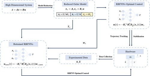
The retrained RBFNN control is experimentally evaluated and compared with the original model-based RBFNN control. A flowchart in Figure 1 summarises the RBFNN control design procedure discussed in the previous sections.

Figure 1. Flowchart of the RBFNN optimal control algorithm with model reduction and transfer learning for linear systems.

6. RBFNN control for linear systems

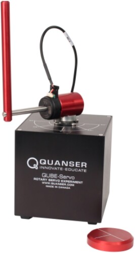
The rotary pendulum is a benchmark dynamic system to study control performance. It is taken as a linear example for the RBFNN control validation due to its compatibility with numerical and experimental evaluation. The Quanser-Servo2 inverted pendulum system in Figure 2 is the hardware to validate the performance of the algorithm. The system has two degrees of freedom. The corresponding state space is four dimensional, which makes the computation of the RBFNN control from the HJB equation more complicated. Note that the RBFNN control is first applied on a simple 2D system to validate its performance on the linear system as shown in Appendix.

Figure 2. Quanser-Servo2 Inverted Pendulum system hardware setup (Quanser, 2022).

6.1. Numerical simulations

The linearised model of the rotary pendulum at the equilibrium point is given by, (50) $\begin{array}{rl}{J}_r\ddot{\theta }+m_p\mathrm{lr}\ddot{\alpha }& =\tau -b_r\dot{\theta }\end{array}$(50) (51) $\begin{array}{rl}{J}_p\ddot{\alpha }+m_p\mathrm{lr}\ddot{\theta }+m_p\mathrm{gl\alpha }& =-b_p\dot{\alpha }\end{array}$(51) where θ is the angle of the rotary arm, α is the angle of the pendulum, τ is the applied torque at the base of the rotary arm. $J_r=m_r{r}^2/3$ is the moment of inertia of the rotary arm with respect to the axis of rotation of the arm, $J_p=m_p{L}_p^2/3$ is the moment of inertial of the pendulum link relative to the axis of rotation of the pendulum, $b_r$ and $b_p$ are the viscous damping coefficients of the rotary arm and the pendulum, respectively. $m_r$ is the mass of the rotary arm and $m_p$ is the mass of the pendulum, $L_p$ is the length of the pendulum and $l=L_p/2$. The nominal values of the rotary pendulum parameters provided by Quanser are listed in Table 1.

Table 1. Parameters of the rotary pendulum system.

Symbol	Description	Value
$m_r$	Mass of rotary arm	0.095 kg
r	Length of rotary arm	0.085 m
$J_r$	Moment inertial of rotary arm	$2.29\times {10}^{-4}\mathrm{kg}\cdot {\mathrm{m}}^2$
$b_r$	Viscous damping of rotary arm	${10}^{-3}\mathrm{N}\cdot \mathrm{m}\cdot \mathrm{s}/\mathrm{rad}$
$m_p$	Mass of pendulum	0.024 kg
$L_p$	Length of pendulum	0.129 m
l	Half length of pendulum	0.0645 m
$J_p$	Moment inertial of pendulum	$1.33\times {10}^{-4}\mathrm{kg}\cdot {\mathrm{m}}^2$
$b_p$	Viscous damping coefficient	$5\times {10}^{-5}\mathrm{N}\cdot \mathrm{m}\cdot \mathrm{s}/\mathrm{rad}$
g	Gravitational acceleration	9.81 $\mathrm{m}\cdot {\mathrm{s}}^2$

The state equations of the linear model in Equations (50(50) $\begin{array}{rl}{J}_r\ddot{\theta }+m_p\mathrm{lr}\ddot{\alpha }& =\tau -b_r\dot{\theta }\end{array}$(50) ) and (51(51) $\begin{array}{rl}{J}_p\ddot{\alpha }+m_p\mathrm{lr}\ddot{\theta }+m_p\mathrm{gl\alpha }& =-b_p\dot{\alpha }\end{array}$(51) ) with the nominal values of the parameters are given by, (52) $\begin{array}{rl}\dot{\mathbf{x}}(t)& =\left[\begin{array}{cccc}0& 0& 1.0& 0\\ 0& 0& 0& 1.0\\ 0& 152.0057& -12.2542& -0.5005\\ 0& 264.3080& -12.1117& -0.8702\end{array}\right]\mathbf{x}(t)\\ & +\left[\begin{array}{c}0\\ 0\\ 50.6372\\ 50.0484\end{array}\right]\tau \end{array}$(52) (53) $\begin{array}{rl}\mathbf{y}(t)& =\left[\begin{array}{cccc}1& 0& 0& 0\\ 0& 1& 0& 0\end{array}\right]\mathbf{x}(t)\end{array}$(53) where $\mathbf{x}=[\theta ,\alpha ,\dot{\theta },\dot{\alpha }{]}^T$ is the state vector of the rotary pendulum. The outputs are the angles of rotary arm θ and pendulum α. In simulations, it is assumed that all the system states are available for the full state feedback control. In experiments, the derivatives of the angle measurements can be obtained through a low pass filter (Quanser, 2022), (54) $\begin{array}{r}H(s)=\frac{50s}{s+50}\end{array}$(54) Model-based balanced truncation and empirical balanced truncation are both applied to the Quanser inverted pendulum system to obtain a reduced order model. The empirical balanced truncation is designed for the stable system with steady state impulse response. However, the empirical balanced truncation has been shown to be a suitable method for systems with unstable modes and non-homogeneous initial conditions due to its data-driven nature (Himpe, 2018). In support of this finding, numerical simulations have demonstrated the applicability of empirical balanced truncation to the Quanser inverted pendulum within a short simulation time $t=1.5\mathrm{s}$ in this study. In this case, due to the instability of the system, the reduced order model obtained from empirical balanced truncation is different from balanced truncation. Details of the reduced order model matrices from model-based and empirical gramians can be found in Table 2.

Table 2. Summary of reduced order model matrices from model-based gramians and empirical gramians.

Model-based gramians	Empirical gramians
$A_r=\left[\begin{array}{ccc}0& -2.0421& 0\\ 0& 13.7774& 0\\ 0& 0& -5.4132\end{array}\right]$	$A_r=\left[\begin{array}{ccc}13.7791& 0.2460& -0.0002\\ -0.2614& -21.9083& 0.0014\\ -0.0011& -0.0389& 0.0842\end{array}\right]$
$B_r=\left[\begin{array}{c}1.1392\\ -0.7163\\ -1.9942\end{array}\right]$	$B_r=\left[\begin{array}{c}-1.0746\\ 1.5235\\ -1.9277\end{array}\right]$
$C_r=\left[\begin{array}{ccc}4.00& 0& 1.9936\\ 0& -1.4653& -0.0477\end{array}\right]$	$C_r=\left[\begin{array}{ccc}-0.4058& -0.9037& -1.6948\\ -0.9951& -1.1802& -0.0585\end{array}\right]$

The Hankel singular values of the rotary pendulum from model-based gramians are shown in Table 3. The first two rows represent the unstable modes of the system with infinite singular values out of the range of the plot. The last two rows represent the stable modes of the system with finite singular values. Table 3 suggests that the first three eigen-modes dominate the system. Hence, the order of the reduced order model is chosen to be r = 3 to approximate the original model for both balanced truncation and empirical balanced truncation.

Table 3. Hankel singular values of the rotary pendulum.

State	Hankel singular value ${\omega }_i$
1	∞
2	∞
3	0.3673
4	0.0304

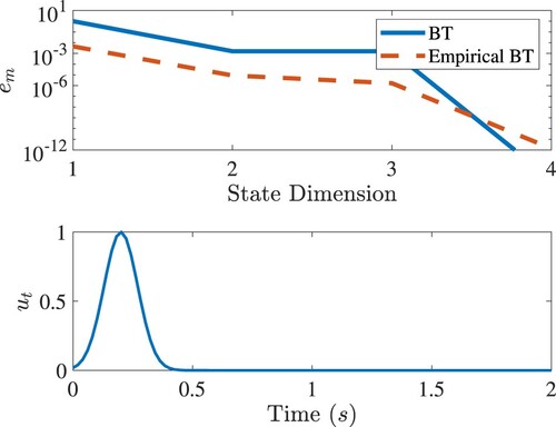
Figure 3 shows the relative output error $e_m$ of the two reduced order models compared to the output of the original system in Equations (47(47) $\begin{array}{r}\begin{array}{rl}& {\mathbf{\Phi }}^{\mathrm{ilm}}(t)=({\mathbf{x}}^{\mathrm{ilm}}(t)-{\overline{\mathbf{x}}}^{\mathrm{ilm}})({\mathbf{x}}^{\mathrm{ilm}}(t)-{\overline{\mathbf{x}}}^{\mathrm{ilm}}{)}^T\\ & {\mathit{\psi }}_{\mathrm{ij}}^{\mathrm{lm}}(t)=({\mathbf{y}}^{\mathrm{ilm}}(t)-{\overline{\mathbf{y}}}^{\mathrm{ilm}}{)}^T({\mathbf{y}}^{\mathrm{jlm}}(t)-{\overline{\mathbf{y}}}^{\mathrm{jlm}})\\ & {\mathbf{T}}_i^T{\mathbf{T}}_i=\mathbf{I},{\mathbf{T}}_i\in {\mathbb{R}}^{n\times n},i=1,\dots ,r\\ & c_i>0,c_i\in \mathbb{R},i=1,\dots ,s\end{array}\end{array}$(47) ) and (48(48) $\begin{array}{r}\mathbf{u}(t)=-{\mathbf{R}}_r^{-1}{\mathbf{B}}_r^T{\mathbf{D}}_{\mathbf{g}}({\mathbf{x}}_r(t)){\mathbf{w}}_r\end{array}$(48) ) when the same input $u_t(t)=e^{-100(t-0.2{)}^2}$ is applied. $e_m$ is defined as (55) $\begin{array}{r}{e}_m=\sqrt{\frac{\sum _{i=1}^{n_s}|\mathbf{y}(i)-{\mathbf{y}}_r(i){|}^2}{\sum _{i=1}^{n_s}|\mathbf{y}(i){|}^2}}\end{array}$(55) where $n_s$ is the number of integration steps and i is the discrete time index, corresponding to the physical time $t=i\mathrm{\Delta t}$. $\mathrm{\Delta }t$ is the integration time step or sample time in experiments. The relative output error of the empirical balanced truncation is less than the model-based balanced truncation as seen in Figure 3. This indicates that the empirical gramians contain more accurate information than the model-based balanced gramians.

Figure 3. Top: Relative output errors of the reduced order model by the balanced truncation and empirical balanced truncation. Below: The input signal.

The LQR control of the original system is taken as a benchmark to compare with the performance of the RBFNN controls designed with the reduced order models. The $\mathbf{Q}$ and $\mathbf{R}$ matrices for the LQR control of the original system and the reduced order models are given by, (56) $\begin{array}{r}\begin{array}{rl}\mathbf{Q}& =\left[\begin{array}{cccc}5& 0& 0& 0\\ 0& 1& 0& 0\\ 0& 0& 1& 0\\ 0& 0& 0& 1\end{array}\right],{\mathbf{Q}}_{\mathrm{bt}}=\left[\begin{array}{ccc}100& 0& 0\\ 0& 1& 0\\ 0& 0& 1\end{array}\right],\\ {\mathbf{Q}}_{\mathrm{ebt}}& =\left[\begin{array}{ccc}100& 0& 0\\ 0& 100& 0\\ 0& 0& 30\end{array}\right],\mathbf{R}={\mathbf{R}}_{\mathrm{bt}}={\mathbf{R}}_{\mathrm{ebt}}=1.\end{array}\end{array}$(56) The sampling region for the RBFNN method with the reduced order model is chosen as $X_s=[-1,1]\times [-1,1]\times [-1,1]$. The means of Gaussian neurons are uniformly distributed in the region $X_g=[-4,4]\times [-4,4]\times [-4,4]$. The standard deviations of Gaussian neurons are ${\sigma }_1={\sigma }_2={\sigma }_3=2.6667$. The number of neurons $N_G=4^3=64$ and the sampling points $N_s=2^3{N}_G$. ${\mathbf{w}}_r$ denotes the trainable weights of the RBFNN for the reduced order model.

We first consider tracking control. The reference signal is chosen as, (57) $\begin{array}{r}{\mathbf{x}}_{\mathrm{ref}}=[{\theta }_r,0,0,0{]}^T\end{array}$(57) After that, the reference in the reduced order model space reads, (58) $\begin{array}{r}{\mathbf{x}}_{\mathrm{re}{f}_r}={\mathbf{T}}_r^{-1}{\mathbf{x}}_{\mathrm{ref}}\end{array}$(58) The optimal control is given Equation (49(49) $\begin{array}{r}\mathbf{u}(t)=-{\mathbf{R}}_r^{-1}{\mathbf{B}}_r^T({\mathbf{D}}_{\mathbf{g}}({\mathbf{x}}_r(t))-{\mathbf{D}}_{\mathbf{g}}({\mathbf{x}}_{\mathrm{re}{f}_r}(t))){\mathbf{w}}_r\end{array}$(49) ). A root mean square (RMS) error is defined to quantify the performance of the tracking control, (59) $\begin{array}{r}{e}_{\mathrm{RMS}}=\sqrt{\frac{1}{n_s}\sum _{i=1}^{n_s}(\theta (i)-{\theta }_r(i){)}^2}\end{array}$(59) We have chosen the time duration of 50 s and integration step $\mathrm{\Delta }t=0.001\mathrm{s}$. Hence, the number of integration steps $n_s=\mathrm{50,000}$.

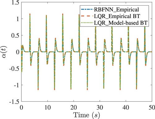
Consider a square wave reference. Figure 4 shows the performance of the controls under consideration. From this figure, it is clear that the RBFNN optimal control has the ability to track the desired trajectory with different reduced order models and shows similar results compared to the LQR control of the original system. The RMS tracking errors of the RBFNN controls based on the model-based BT and empirical BT reduced order model and the LQR are 3.13, 3.16 and 3.71, respectively. Figures 5 and 6 show the comparisons of empirical RBFNN with the LQR control designed with the empirical BT and model-based BT.

Figure 4. Tracking the square wave of the rotary army in simulations. In the legend, ‘LQR’ denotes the LQR control designed with the original model; ‘RBFNN’ denotes the RBFNN control designed with the model-based BT; ‘Empirical RBFNN’ denotes the RBFNN control designed with the empirical BT.

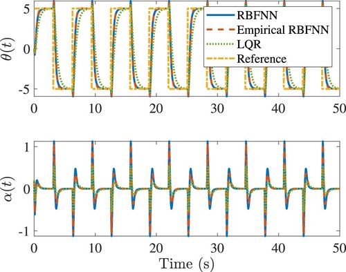
Figure 5. Comparisons of tracking response $\theta (t)$ of the rotary army in simulations. In the legend, ‘RBFNN_Empirical’ denotes the RBFNN control designed with the empirical BT; ‘LQR_Empirical BT’ denotes the LQR control designed with the empirical BT; ‘LQR_Model-based BT’ denotes the LQR control designed with the model-based BT.

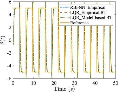
Figure 6. Comparisons of tracking response $\alpha (t)$ of the rotary army in simulations. Legends are the same as in Figure 5.

6.2. A summary

The rotary pendulum model is inherently unstable. Finding an initial stabilising random control to enable policy iteration convergence in RBFNN control design using the original model is a challenging mask. We have discovered that it is much easier to find an initial stabiliser for the reduced order system to make the policy iteration converge. This is an interesting phenomenon that deserves further investigation.

The RBFNN controls are pre-trained and can be implemented in the hardware. In the following, experimental data of the RBFNN controls were collected from the Quanser-Servo2 inverted pendulum and further improve the performance of these controls with the transfer leaning technique.

6.3. Experimental validation

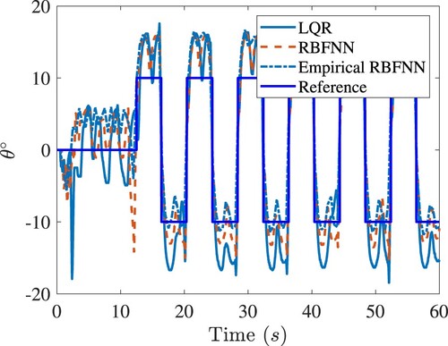
Two control experiments of pendulum balancing and rotary arm trajectory tracking are carried out on the Quanser-Servo2 Inverted Pendulum system with the RBFNN optimal controllers. All the experiments are done with Quanser HIL and MATLAB Simulink. The sample time is set to $\mathrm{\Delta }t=0.002\mathrm{s}$. The tests run for $60\mathrm{s}$. The closed-loop responses tracking the square wave as the reference signal for rotary arm are shown in Figure 7. Both the RBFNN optimal controls deliver better tracking performance than the LQR control.

Figure 7. The closed-loop tracking responses $\theta (t)$ of the rotary arm of Quanser-Servo2. Legends are the same as in Figure 4.

Experimental data have been obtained to improve the control performance through retraining the neural networks. The transient responses of the system have been eliminated and the remaining data have been restricted to the time interval $t\in [3,12]\mathrm{s}$ for the model-based BT design and $t\in [3,10]\mathrm{s}$ for the empirical BT design. The effect of retraining on balancing control is shown in Figure 8. It is clear that the retraining of the neural networks with experimental data benefits the control designed with the empirical BT most.

Figure 8. The closed-loop responses $\theta (t)$ of the rotary arm under various controls for balancing the inverted pendulum of Quanser-Servo2. Top: Responses before retraining. Bottom: Responses after retraining. Legends are the same as in Figure 4.

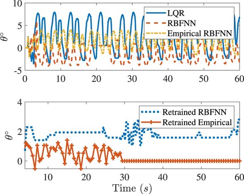
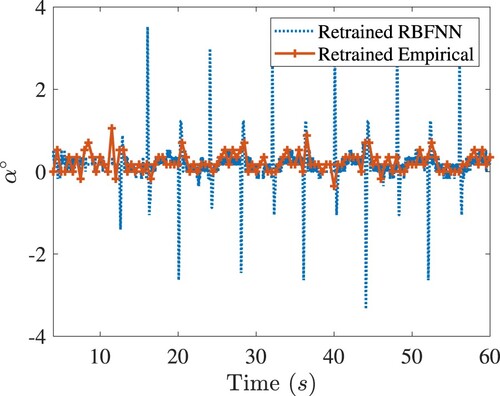
Figure 9 shows the effect of retraining on tracking control. Compared to Figure 7, the performance improvement of tracking the angle $\theta (t)$ is obvious. Moreover, suppression of many spiky responses of $\alpha (t)$ angle in Figure 10 is a strong evidence of the benefits of retraining.

Figure 9. The closed-loop tracking response $\theta (t)$ of the rotary arm of Quanser-Servo2. Legends are the same as in Figure 4.

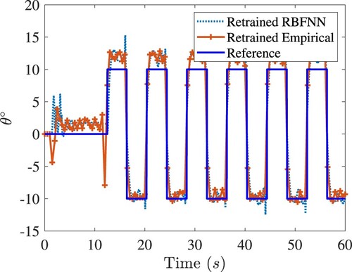
Figure 10. The closed-loop response $\alpha (t)$ of the pendulum in the rotary arm tracking control of Quanser-Servo2. Legends are the same as in Figure 4.

A measure of control effort is defined in terms of the integrated absolute control voltage $v(t)$, which is given by, (60) $\begin{array}{r}{u}_{\mathrm{effort}}=\sum _{i=1}^{n_s}|v(i)|\end{array}$(60) Table 4 lists the RMS tracking errors and the control effort with a consideration of the effects of retraining. It is worth noting that the RBFNN control designed with the empirical BT has the smallest RMS error.

Table 4. Summary of control performance for LQR, RBFNN, empirical RBFNN, retrained RBFNN and retrained empirical RBFNN.

Case	Algorithm	$e_{\mathrm{RMS}}$	$u_{\mathrm{effort}}$
	LQR	4.54	4667.64
	RBFNN	2.31	4080.89
Stabilization	Retrained RBFNN	1.83	2769.3
	Empirical RBFNN	2.86	4343.8
	Retrained Empirical	0.57	3210.1
	LQR	4.67	7410.1
Trajectory	RBFNN	4.08	7468.4
Tracking	Retrained RBFNN	2.77	6667.5
	Empirical RBFNN	4.34	6794.8
	Retrained Empirical	3.21	8380.3

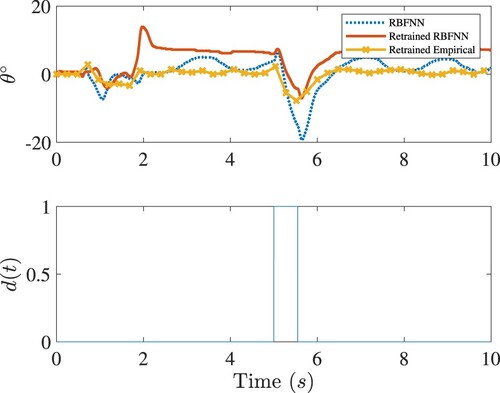
The robustness of the balancing control to disturbance is also investigated through experimental evaluation. A torque disturbance $d(t)$ is injected at $t\in [5,5.5]\mathrm{s}$ by introducing a voltage pulse to the motor. Figure 11 shows that the retrained empirical RBFNN has superb robustness to disturbance compared to the other two controls.

Figure 11. Robustness comparisons of all the controls under consideration. Top: The closed-loop angle response $\theta (t)$ of the rotary arm in balancing control of Quanser-Servo2. Bottom: Disturbance $d(t)$. Legends are the same as in Figure 4.

7. Nonlinear controls

The RBFNN method is now applied to obtain optimal controls for nonlinear systems and study the robustness of RBFNN control with respect to the model uncertainty.

7.1. A second order system

Neural networks with polynomial activation functions (Poly-NN) have been applied to find the solutions of the HJB equation. This has been a popular example in the literature (L. Chen et al., 2023; Du et al., 2024; Lin et al., 2024; Luo et al., 2014; Modares & Lewis, 2014; Qin et al., 2023; Yang et al., 2014). In the following, the performance of the optimal control expressed in terms of the RBFNN with Gaussian neurons is compared with that of the polynomial neural networks (Poly-NN). Consider a second order nonlinear system, (61) $\begin{array}{r}\begin{array}{rl}{\dot{x}}_1& =x_1+x_2-x_1(x_1^2+x_2^2)\\ {\dot{x}}_2& =-x_1+x_2-x_2(x_1^2+x_2^2)+u\end{array}\end{array}$(61) We take the Poly-NN reported in Abu-Khalaf and Lewis (2005) to compare with the proposed RBFNN control. No control constraints are imposed in the comparison. Both the neural networks are trained in the sampling region $X_s\in [-1,1]\times [-1,1]$ and applied to two regions $X_{s1}\in [-1,1]\times [-1,1]$ and $X_{s2}\in [-2,2]\times [-2,2]$ to check their ability to provide good control performance beyond the training region. This is a way to study the generalisation of the neural networks.

The Poly-NN has 24 neurons where the RBFNN has $N_G=5\times 5=25$ neurons. The sampling points are $N_s=2^2{N}_G$ for both neural networks. The standard deviations of Gaussian neurons are ${\sigma }_1={\sigma }_2=0.75$. To investigate robustness of the controls, a disturbance $d(t)$ is considered to each state of the system as shown in Figure 12. (62) $\begin{array}{r}d(t)=\{\begin{array}{ll}1+g(t),& 10\le t\le 11\\ 5+g(t),& 20\le t\le 21\\ 10+g(t),& 30\le t\le 31\\ g(t),& \mathrm{else}\end{array}\end{array}$(62) where $g(t)$ is the Gaussian white noise. Its signal-to-noise (SNR) ratio is 50 dB.

Figure 12. Disturbances to the second order nonlinear system.

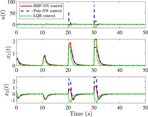
The closed-loop responses are shown in Figure 13. Within the training region $X_s\in [-1,1]\times [-1,1]$, the RBFNN, Poly-NN and LQR controls have about the same performance when the system starts from the same initial condition ${\mathbf{x}}_0=[0.5,0.5{]}^T$ and is subject to the disturbance $d(t)$. Note that the LQR control is designed based on the linearised system. When the disturbance becomes stronger, the RBFNN control can still stabilise the system with reasonable effort. However, the Poly-NN control performs poorly.

Figure 13. Performance comparison of RBFNN, Poly-NN control and LQR controls for the nonlinear system in Equation (61(61) $\begin{array}{r}\begin{array}{rl}{\dot{x}}_1& =x_1+x_2-x_1(x_1^2+x_2^2)\\ {\dot{x}}_2& =-x_1+x_2-x_2(x_1^2+x_2^2)+u\end{array}\end{array}$(61) ). Top: The control $u(t)$. Middle: The response $x_1(t)$. Bottom: The response $x_2(t)$.

This is due to the well-known fact that polynomials generate large extrapolation errors in regression applications. We compare both the controls in the training region $X_{s1}$ and in a larger region $X_{s2}$ in Figure 14. As seen from the figure, the Poly-NN control grows unbounded quickly outside the training region and can no longer stabilise the system, while the RBFNN control remains bounded and can still stabilise the system in this larger region. As a matter of fact, the RBFNN control will remain bounded and approach zero at locations far away from the training region, because all the Gaussian neurons with means in the training region decrease exponentially.

Figure 14. Comparison of spatial distribution of RBFNN and Poly-NN optimal controls u as a function of the state $\mathbf{x}$. Left: The control $u(\mathbf{x})$ plotted in the training region $X_{s1}\in [-1,1]\times [-1,1]$. Right: The control $u(\mathbf{x})$ plotted beyond the training region into the larger region $X_{s2}\in [-2,2]\times [-2,2]$.

7.2. Duffing system

Consider the Duffing system as another example to test the robustness of RBFNN controller with changing parameters, (63) $\begin{array}{r}\left[\begin{array}{c}{\dot{x}}_1\\ {\dot{x}}_2\end{array}\right]=\left[\begin{array}{cc}0& 1\\ 0& -0.1\end{array}\right]\left[\begin{array}{c}{x}_1\\ x_2\end{array}\right]+\left[\begin{array}{c}0\\ 1\end{array}\right]u+\left[\begin{array}{c}0\\ \beta \end{array}\right]x_1^3\end{array}$(63) The sampling region is $X_s\in [-2,2]\times [-8,8]$. Corresponding to the sampling region, the means of Gaussian neurons are uniformly distributed in the region $X_g\in [-3,3]\times [-9,9]$.

We take $\beta =2$ as the nominal value and allow β to vary in a known range $1\le \beta \le 6$. Both the RBFNN and LQR controls are designed with the nominal value of β. Note that the LQR control is designed for the linearised system at $\beta =2$. The performance index J of the LQR design is defined as, (64) $\begin{array}{r}J(\mathbf{x},\mathbf{u})=\frac{1}{2}\sum _{k=0}^{n_s}[{\mathbf{x}}^T(k)\mathbf{Qx}(k)+R{u}^2(k)].\end{array}$(64) where k is the discrete time index, and $n_s$ is number of integration steps of the simulation. The matrices are given by (65) $\begin{array}{r}\mathbf{Q}=\left[\begin{array}{cc}10& 0\\ 0& 10\end{array}\right],R=1\end{array}$(65) We have chosen $n_s=1000$. The integration time step is $\mathrm{\Delta }t=0.01\mathrm{s}$. We simulate the closed-loop system starting from the same initial condition ${\mathbf{x}}_0=[0.7,0.7{]}^T$.

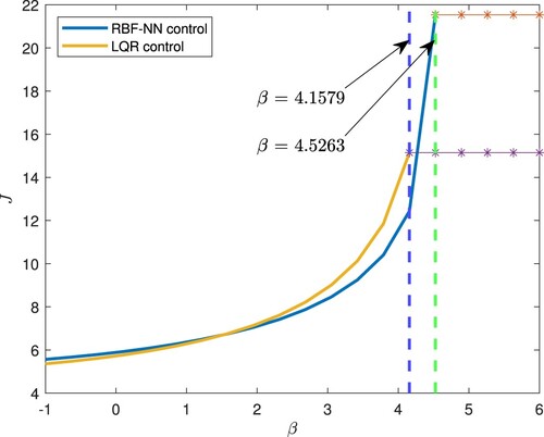
The index J is used to evaluate the performance of both the RBFNN and LQR controls. Figure 15 shows the performance index J as a function of β for both the RBFNN and LQR controls. When the actual value of β is less than the nominal value 2, the linearised model of the system remains valid. As a result, the LQR control is slightly better than the RBFNN control. However, when $\beta >2$, the linearised model at $\beta =2$ becomes less accurate, resulting in poor performance of the LQR control compared with the RBFNN control. When β reaches a critical value ${\beta }_{\mathrm{cr}}$, marked by the vertical lines in the figure, the closed-loop system becomes unstable and the performance index J grows unbounded. For the LQR control, ${\beta }_{\mathrm{cr}}=4.1579$, while for the RBFNN control, ${\beta }_{\mathrm{cr}}=4.5263$. This is a quantitative measurement of robustness to model uncertainty.

Figure 15. Robustness of the RBFNN and LQR controls with respect to the model uncertainty β. The vertical dash lines mark the critical value of β, beyond which the closed-loop system becomes unstable.

Finally, we should point out that the RBFNN with one hidden layer can find optimal controls with good performance and robustness for nonlinear dynamic systems. The design of RBFNN itself is not optimised in this study. However, there are studies on how to design RBFNN in the literature, such as ErrCor algorithm (Yu et al., 2011), hierarchical growing strategy (GGAP algorithm) (Sundararajan et al., 1999), MRAN algorithm (Kadirkamanathan & Niranjan, 1993), resource allocation algorithm (Platt, 1991), and adaptive RBF algorithms (Alwardi et al., 2013, 2012; González-Casanova et al., 2009). These algorithms can be considered for optimal design of RBFNN architecture in the future study.

Remark 7.1

This paper proposes a method to compute the solutions of nonlinear optimal control expressed in terms of the RBFNN with Gaussian activation functions for multi-degree-of-freedom dynamic systems. Combined with model reduction and transfer learning algorithm, the computational efficiency and the control performance have been significantly improved. Extensive numerical simulations and experimental studies show that the RBFNN offer excellent control performance and much-improved robustness to disturbances and model uncertainties. It is worth mentioning that the RBFNN control delivers the same performance as the LQR control for the LTI system. Our previous work (Zhao & Sun, 2022) indicates that the BT reduction for the LTI system leads to significant performance improvements compared to the LQR control. For nonlinear systems, such as the Duffing system shown in Section 7.2, the nonlinear optimal control solution from RBFNN shows improved robustness compared to the LQR control for the linearised system.

Remark 7.2

Our early work (Gholami et al., 2023) indicates that other neural networks, such as multi-layer perceptron, are not suitable for solving the HJB equation. In the paper (Gholami et al., 2023), we adopted a two-layer perceptron neural networks with hyperbolic tangent functions to approximate the derivative of the value function in the HJB equation. However, it is very time-consuming to solve the optimal control. Additionally, the structure of multi-layer perceptron is not beneficial to obtain the explicit expression of the optimal coefficient in Equation (35(35) $\begin{array}{r}\mathbf{w}(k+1)=-{\mathbf{A}}_g^{-1}(k)\mathbf{b}(k)\end{array}$(35) ), which is one of the reasons why the proposed RBFNN method is efficient and accurate.

8. Conclusion

This paper has presented a RBFNN optimal control approach with Gaussian neurons. Instead of analytically solving the HJB equation, the RBFNN computes the optimal control solution with high efficiency. The RBFNN optimal controls are obtained off-line in the state space for both linear and nonlinear dynamic systems. Extensive simulations and experimental studies have been presented and suggest that the RBFNN optimal control can deliver excellent performance and robustness. We have also implemented model reduction techniques to reduce computational burden of the RBFNN design when solving HJB equations in high dimensional state space, and explored transfer learning concept to update the coefficients of the neural networks with new experimental data leading to a better control performance in experiments. The extensive numerical simulations and experimental validations prove that the neural networks with one-hidden layer have significant potential for different electro-mechanical systems, particularly high-dimensional nonlinear dynamical systems. The work demonstrates that with a limited number of neurons, the RBFNN can be successfully implemented on the micro-controller hardware. Moreover, a comparative analysis between RBFNN and other similar machine learning algorithms, such as LANN-SVD algorithm can be an interesting research topic for the future.

Disclosure statement

No potential conflict of interest was reported by the author(s).

Additional information

Funding

This material is based upon work supported by the AI Research Institutes program supported by NSF and USDA-NIFA under the AI Institute: Agricultural AI for Transforming Workforce and Decision Support (AgAID) [award number 2021-67021-35344]. Partial support to the work was from a National Natural Science Foundation of China [grant number 11972070].

Appendix. A linear 2D system

In this section, we adopt a linear 2D system as an example to validate the performance of the RBFNNs control presented in Sections 2 and 3. It is noted that the model reduction algorithm is not applied since the system has a low dimension and requires reasonably low computational cost. The linear 2D system is defined as, (A1) $\begin{array}{r}\left[\begin{array}{c}{\dot{x}}_1\\ {\dot{x}}_2\end{array}\right]=\left[\begin{array}{cc}0& 1\\ -\frac{k}{m}& -\frac{c}{m}\end{array}\right]\left[\begin{array}{c}{x}_1\\ x_2\end{array}\right]+\left[\begin{array}{c}0\\ 1\end{array}\right]u\end{array}$(A1) where m = 1, c = 2 and k = 1. The region to distribute Gaussian neurons is chosen as $X_{1g}\times X_{2g}=[-2,2]\times [-6,6]$. The region to sample points for integration is chosen as $X_{1s}\times X_{2s}=[-1,1]\times [-3,3]$. The number of neurons $N_G\times N_G$ are $9\times 9$ and the sampling points are $2N_G\times 2N_G$. $\mathbf{Q}$ and $\mathbf{R}$ are chosen as, (A2) $\begin{array}{r}\mathbf{Q}=\left[\begin{array}{cc}10& 0\\ 0& 10\end{array}\right],\mathbf{R}=1\end{array}$(A2) The results are shown in Figure A1. From Figure A1, we can see that RBFNNs can find the exactly same optimal solution as LQR for the linear 2D system.

Figure A1. Comparison of RBFNNs and LQR control performances for the linear 2D system. Top: Control $u(t)$. Middle: Response $x_1(t)$. Bottom: Response $x_2(t)$. The initial condition of the system is $\mathbf{x}(0)=[1,1{]}^T$.

References

- Abu-Khalaf, M., & Lewis, F. L. (2005). Nearly optimal control laws for nonlinear systems with saturating actuators using a neural network HJB approach. Automatica, 41(5), 779–791. https://doi.org/10.1016/j.automatica.2004.11.034
- Alwardi, H., Wang, S., & Jennings, L. S. (2013). An adaptive domain decomposition method for the Hamilton–Jacobi–Bellman equation. Journal of Global Optimization, 56(4), 1361–1373. https://doi.org/10.1007/s10898-012-9850-2
- Alwardi, H., Wang, S., Jennings, L. S., & Richardson, S. (2012). An adaptive least-squares collocation radial basis function method for the HJB equation. Journal of Global Optimization, 52(2), 305–322. https://doi.org/10.1007/s10898-011-9667-4
- Borovykh, A., Kalise, D., Laignelet, A., & Parpas, P. (2022). Data-driven initialization of deep learning solvers for Hamilton–Jacobi–Bellman PDEs. IFAC-PapersOnLine, 55(30), 168–173. https://doi.org/10.1016/j.ifacol.2022.11.047
- Chen, J.-S., Hillman, M., & Chi, S.-W. (2017). Meshfree methods: Progress made after 20 years. Journal of Engineering Mechanics, 143(4), 04017001. https://doi.org/10.1061/(ASCE)EM.1943-7889.0001176
- Chen, L., Dong, C., & Dai, S.-L. (2023). Adaptive optimal consensus control of multiagent systems with unknown dynamics and disturbances via reinforcement learning. IEEE Transactions on Artificial Intelligence. https://doi.org/10.1109/TAI.2023.3324895
- Cheng, T., Lewis, F. L., & Abu-Khalaf, M. (2007a). A neural network solution for fixed-final time optimal control of nonlinear systems. Automatica, 43(3), 482–490. https://doi.org/10.1016/j.automatica.2006.09.021
- Cheng, T., Lewis, F. L., & Abu-Khalaf, M. (2007b). Fixed-final-time-constrained optimal control of nonlinear systems using neural network HJB approach. IEEE Transactions on Neural Networks, 18(6), 1725–1737. https://doi.org/10.1109/TNN.2007.905848
- Crandall, M. G., & Lions, P.-L. (1983). Viscosity solutions of Hamilton–Jacobi equations. Transactions of the American Mathematical Society, 277(1), 1–42. https://doi.org/10.1090/tran/1983-277-01
- Darbon, J., Dower, P. M., & Meng, T. (2021). Neural network architectures using min plus algebra for solving certain high dimensional optimal control problems and Hamilton–Jacobi PDEs. Preprint. arXiv:2105.03336.
- Darbon, J., & Osher, S. (2016). Algorithms for overcoming the curse of dimensionality for certain Hamilton–Jacobi equations arising in control theory and elsewhere. Research in the Mathematical Sciences, 3(1), 1–26. https://doi.org/10.1186/s40687-016-0068-7
- Djeridane, B., & Lygeros, J. (2006). Neural approximation of PDE solutions: An application to reachability computations. In Proceedings of the 45th IEEE Conference on Decision and Control (pp. 3034–3039). San Diego, CA, USA: IEEE.
- Doya, K. (2000). Reinforcement learning in continuous time and space. Neural Computation, 12(1), 219–245. https://doi.org/10.1162/089976600300015961
- Du, Y., Jiang, B., & Ma, Y. (2024). Adaptive optimal sliding-mode fault-tolerant control for nonlinear systems with disturbances and estimation errors. Complex & Intelligent Systems, 10, 1087–1101.
- Gawronski, W., & Juang, J.-N. (1990). Model reduction in limited time and frequency intervals. International Journal of Systems Science, 21(2), 349–376. https://doi.org/10.1080/00207729008910366
- Gholami, A., Sun, J.-Q., & Ehsani, R. (2023). Neural networks based optimal tracking control of a delta robot with unknown dynamics. International Journal of Control, Automation and Systems, 21(10), 3382–3390. https://doi.org/10.1007/s12555-022-0745-9
- González-Casanova, P., Muñoz-Gómez, J. A., & Rodríguez-Gómez, G. (2009). Node adaptive domain decomposition method by radial basis functions. Numerical Methods for Partial Differential Equations: An International Journal, 25(6), 1482–1501. https://doi.org/10.1002/num.v25:6
- Greif, C. (2017). Numerical methods for Hamilton–Jacobi–Bellman equations [PhD thesis]. University of Wisconsin, Milwaukee].
- Grundel, S., Himpe, C., & Saak, J. (2019). On empirical system gramians. PAMM, 19(1), e201900006. https://doi.org/10.1002/pamm.v19.1
- Gugercin, S., & Antoulas, A. C. (2004). A survey of model reduction by balanced truncation and some new results. International Journal of Control, 77(8), 748–766. https://doi.org/10.1080/00207170410001713448
- Guo, Y., Shi, H., Kumar, A., Grauman, K., Rosing, T., & Feris, R. (2019). Spottune: Transfer learning through adaptive fine-tuning. In Proceedings of the IEEE/CVF Conference on Computer Vision and Pattern Recognition (pp. 4805–4814). Long Beach, CA, USA.
- Han, J., Jentzen, A., & E, W. (2018). Solving high-dimensional partial differential equations using deep learning. Proceedings of the National Academy of Sciences, 115(34), 8505–8510. https://doi.org/10.1073/pnas.1718942115
- Heinkenschloss, M., Reis, T., & Antoulas, A. C. (2011). Balanced truncation model reduction for systems with inhomogeneous initial conditions. Automatica, 47(3), 559–564. https://doi.org/10.1016/j.automatica.2010.12.002
- Himpe, C. (2018). Emgr – the empirical gramian framework. Algorithms, 11(7), 91. https://doi.org/10.3390/a11070091
- Huang, Y., & Kramer, B. (2020). Balanced reduced-order models for iterative nonlinear control of large-scale systems. IEEE Control Systems Letters, 5(5), 1699–1704. https://doi.org/10.1109/LCSYS.7782633
- Jiang, F., Chou, G., Chen, M., & Tomlin, C. J. (2016). Using neural networks to compute approximate and guaranteed feasible Hamilton–Jacobi–Bellman PDE solutions. Preprint. arXiv:1611.03158.
- Kadirkamanathan, V., & Niranjan, M. (1993). A function estimation approach to sequential learning with neural networks. Neural Computation, 5(6), 954–975. https://doi.org/10.1162/neco.1993.5.6.954
- Lagaris, I. E., Likas, A. C., & Papageorgiou, D. G. (2000). Neural-network methods for boundary value problems with irregular boundaries. IEEE Transactions on Neural Networks, 11(5), 1041–1049. https://doi.org/10.1109/72.870037
- Laub, A., Heath, M., Paige, C., & Ward, R. (1987). Computation of system balancing transformations and other applications of simultaneous diagonalization algorithms. IEEE Transactions on Automatic Control, 32(2), 115–122. https://doi.org/10.1109/TAC.1987.1104549
- Lewis, F., Jagannathan, S., & Yesildirak, A. (1998). Neural network control of robot manipulators and non-linear systems. CRC Press.
- Lin, J., Zhao, B., Liu, D., & Wang, Y. (2024). Dynamic compensator-based near-optimal control for unknown nonaffine systems via integral reinforcement learning. Neurocomputing, 564, 126973. https://doi.org/10.1016/j.neucom.2023.126973
- Liu, D., Li, H., & Wang, D. (2014). Online synchronous approximate optimal learning algorithm for multi-player non-zero-sum games with unknown dynamics. IEEE Transactions on Systems, Man, and Cybernetics: Systems, 44(8), 1015–1027. https://doi.org/10.1109/TSMC.2013.2295351
- Luo, B., Wu, H.-N., Huang, T., & Liu, D. (2014). Data-based approximate policy iteration for affine nonlinear continuous-time optimal control design. Automatica, 50(12), 3281–3290. https://doi.org/10.1016/j.automatica.2014.10.056
- Medagam, P. V., & Pourboghrat, F. (2009). Optimal control of nonlinear systems using RBF neural network and adaptive extended Kalman filter. In American Control Conference (pp. 355–360). St. Louis, MO, USA: IEEE.
- Meyn, S. (2022). Control systems and reinforcement learning. Cambridge University Press.
- Modares, H., & Lewis, F. L. (2014). Optimal tracking control of nonlinear partially-unknown constrained-input systems using integral reinforcement learning. Automatica, 50(7), 1780–1792. https://doi.org/10.1016/j.automatica.2014.05.011
- Modares, H., Lewis, F. L., & Naghibi-Sistani, M.-B. (2014). Integral reinforcement learning and experience replay for adaptive optimal control of partially-unknown constrained-input continuous-time systems. Automatica, 50(1), 193–202. https://doi.org/10.1016/j.automatica.2013.09.043
- Munos, R., Baird, L. C., & Moore, A. W. (1999). Gradient descent approaches to neural-net-based solutions of the Hamilton–Jacobi–Bellman equation. In Proceedings of International Joint Conference on Neural Networks (Vol. 3, pp. 2152–2157). Washington, DC, USA: IEEE.
- Nakamura-Zimmerer, T., Gong, Q., & Kang, W. (2020). A causality-free neural network method for high-dimensional Hamilton–Jacobi–Bellman equations. In 2020 American Control Conference (pp. 787–793). Denver, CO, USA: IEEE.
- Nakamura-Zimmerer, T., Gong, Q., & Kang, W. (2021). Adaptive deep learning for high-dimensional Hamilton–Jacobi–Bellman equations. SIAM Journal on Scientific Computing, 43(2), A1221–A1247. https://doi.org/10.1137/19M1288802
- Nakamura-Zimmerer, T. E. (2022). A deep learning framework for optimal feedback control of high-dimensional nonlinear systems [Thesis]. UC Santa Cruz.
- Park, J., & Sandberg, I. W. (1991). Universal approximation using radial-basis-function networks. Neural Computation, 3(2), 246–257. https://doi.org/10.1162/neco.1991.3.2.246
- Pernebo, L., & Silverman, L. (1982). Model reduction via balanced state space representations. IEEE Transactions on Automatic Control, 27(2), 382–387. https://doi.org/10.1109/TAC.1982.1102945
- Phillips, J., Daniel, L., & Silveira, L. M. (2022). Guaranteed passive balancing transformations for model order reduction. In Proceedings of the 39th Annual Design Automation Conference (pp. 52–57). New Orleans, LA, USA.
- Platt, J. (1991). A resource-allocating network for function interpolation. Neural Computation, 3(2), 213–225. https://doi.org/10.1162/neco.1991.3.2.213
- Qin, C., Qiao, X., Wang, J., Zhang, D., Hou, Y., & Hu, S. (2023). Barrier-critic adaptive robust control of nonzero-sum differential games for uncertain nonlinear systems with state constraints. IEEE Transactions on Systems, Man, and Cybernetics: Systems, 54, 50–63.
- Quanser (2022). QUBE-Servo2. https://www.quanser.com/products/qube-servo-2/
- Saridis, G. N., & Lee, C.-S. G. (1979). An approximation theory of optimal control for trainable manipulators. IEEE Transactions on Systems, Man, and Cybernetics, 9(3), 152–159. https://doi.org/10.1109/TSMC.1979.4310171
- Silverman, B. (2018). Density estimation for statistics and data analysis. CRC Press.
- Singh, A. K., & Hahn, J. (2005). On the use of empirical gramians for controllability and observability analysis. In Proceedings of the American Control Conference (pp. 140–141). Portland, OR, USA: IEEE.
- Sirignano, J., & Spiliopoulos, K. (2018). DGM: A deep learning algorithm for solving partial differential equations. Journal of Computational Physics, 375, 1339–1364. https://doi.org/10.1016/j.jcp.2018.08.029
- Stefansson, E., & Leong, Y. P. (2016). Sequential alternating least squares for solving high dimensional linear Hamilton–Jacobi–Bellman equation. In Proceedings of IEEE/RSJ International Conference on Intelligent Robots and Systems (IROS) (pp. 3757–3764). Daejeon, Korea (South).
- Sun, J. Q., & Hsu, C. S. (1988). A statistical study of generalized cell mapping. Journal of Applied Mechanics, 55, 694–701. https://doi.org/10.1115/1.3125851
- Sundararajan, N., Saratchandran, P., & Lu, Y. W. (1999). Radial basis function neural networks with sequential learning: MRAN and its applications (Vol. 11). World Scientific.
- Tassa, Y., & Erez, T. (2007). Least squares solutions of the HJB equation with neural network value-function approximators. IEEE Transactions on Neural Networks, 18(4), 1031–1041. https://doi.org/10.1109/TNN.2007.899249
- Wang, X., Jiang, J., Hong, L., & Sun, J.-Q. (2022a). First-passage problem in random vibrations with radial basis function neural networks. Journal of Vibration and Acoustics, 144(5), 051014. https://doi.org/10.1115/1.4054437
- Wang, X., Jiang, J., Hong, L., & Sun, J.-Q. (2022b). Stochastic bifurcations and transient dynamics of probability responses with radial basis function neural networks. International Journal of Non-Linear Mechanics, 147, 104244. https://doi.org/10.1016/j.ijnonlinmec.2022.104244
- Wang, X., Jiang, J., Hong, L., Zhao, A., & Sun, J.-Q. (2023). Radial basis function neural networks solution for stationary probability density function of nonlinear stochastic systems. Probabilistic Engineering Mechanics, 71, 103408. https://doi.org/10.1016/j.probengmech.2022.103408
- Wu, Y., Hamroun, B., Le Gorrec, Y., & Maschke, B. (2020). Reduced order LQG control design for infinite dimensional port Hamiltonian systems. IEEE Transactions on Automatic Control, 66(2), 865–871. https://doi.org/10.1109/TAC.9
- Wu, Y., Wang, H., Zhang, B., & Du, K.-L. (2012). Using radial basis function networks for function approximation and classification. ISRN Applied Mathematics, 2012, 1–34. https://doi.org/10.5402/2012/324194
- Yang, X., Liu, D., & Wang, D. (2014). Reinforcement learning for adaptive optimal control of unknown continuous-time nonlinear systems with input constraints. International Journal of Control, 87(3), 553–566. https://doi.org/10.1080/00207179.2013.848292
- Yegorov, I., & Dower, P. M. (2021). Perspectives on characteristics based curse-of-dimensionality-free numerical approaches for solving Hamilton–Jacobi equations. Applied Mathematics & Optimization, 83(1), 1–49. https://doi.org/10.1007/s00245-018-9509-6
- Yu, H., Xie, T., Paszczyñski, S., & Wilamowski, B. M. (2011). Advantages of radial basis function networks for dynamic system design. IEEE Transactions on Industrial Electronics, 58(12), 5438–5450. https://doi.org/10.1109/TIE.2011.2164773
- Zhang, D., Liu, W., Qin, C., & Chen, H. (2016). Adaptive RBF neural-networks control for discrete nonlinear systems based on data. In Proceedings of the 12th World Congress on Intelligent Control and Automation (pp. 2580–2585). Guilin, China: IEEE.
- Zhang, W., Shen, J., Ye, X., & Zhou, S. (2022). Error model-oriented vibration suppression control of free-floating space robot with flexible joints based on adaptive neural network. Engineering Applications of Artificial Intelligence, 114, 105028. https://doi.org/10.1016/j.engappai.2022.105028
- Zhao, A., & Sun, J.-Q. (2022). Control for stability improvement of high-speed train bogie with a balanced truncation reduced order model. Vehicle System Dynamics, 60(12), 4343–4363. https://doi.org/10.1080/00423114.2021.2025408