Invariance-based control for cyber-physical electrical distribution grids

Abstract

Voltage control in low-voltage distribution grids gain importance due to integration of renewable energies and introduction of smart grids. However, the presence of disturbances and communication non-idealities make the problem hard to solve. In addition, lack of integration of converter-based devices caused non-controllability of the grid. In this paper, an updated invariance-based control approach is presented to address these shortcomings. The updated version of the invariance method addresses the non-controllability of the system. In addition, the control approach is discussed in a hybrid formalism in which the long update intervals of the communications are considered. Finally, results show the effectiveness of the approach.

Keywords:

• Distribution grid
• hybrid systems
• invariance-based control
• voltage control

1. Introduction

The transition from conventional grids toward smart grids makes the low-voltage distribution grid an active component of the electrical grid. In this process, renewable energy resources and energy storage devices are introduced to the grid. On the other hand, smart meters (SMs) and communication devices are also integrated into the distribution grid.

Due to the stochastic nature of the renewable energy resources and the increase in consumption, voltage control becomes increasingly important. On the bright side, renewable energy resources are connected to the grid via power electronic interfaces. As a result, controllability of the grid is increased.

Communications can play a crucial role in coordination between controllable units, SMs, and centralised control units. In Bolognani et al. (2019), an analysis which shows the necessity of communication for voltage control in distribution grids has been presented. It is important to mention that the bandwidth of communication is very low; therefore, the process of data collection from SMs takes a long time (Kemal et al., 2020). It is worth mentioning that the slow communications is due to geographically vast area and the number of consumers in the grid.

Understanding the necessity of voltage control in low-voltage distribution grids, it is also important to mention two main challenges. First of all, although the controllability of the grid is increased, still not every node is controllable. It means that there are not controllable devices in every node, and their voltage cannot be tuned to a desired reference. The second problem is communication limitations that make the problem cumbersome. These limitations can be but are not limited to bandwidth, delay, and packet losses.

In Yeh et al. (2012), an optimisation algorithm has been presented to deal with voltage fluctuations and power losses. In addition, an adaptive algorithm has been suggested to select between voltage fluctuations and power losses. Other optimisation methods have been presented in Su et al. (2014) and Dall'Anese et al. (2014) to deal with voltage fluctuations. In Mahmoud Lehtonen (2020), a three level approach based on sensitivity of voltage to active and reactive power has been presented. The algorithm considers local control, area control, and coordinated control, and in each level, different time resolutions for communication are considered. Droop-based approaches have been presented in Chong et al. (2019a, 2019b) in a fully controlled distribution grid. Droop methods contain different bounds in each method. Finally, heuristic methods such as genetic algorithm and artificial neural networks have been used in Li et al. (2019) and Juamperez et al. (2014) to deal with the voltage control problem.

The infeasibility of regulating all the voltage magnitudes to the desired reference using reactive power control leads us to consider a desired set for voltages. In other words, the objective is for the voltages to remain within predetermined boundaries. Having a desired set for the states of the system and the goal of keeping the states in the set is referred to the invariant-based control concept. In this paper, a polyhedral set is defined for the states as the invariant set, and an invariance-based method is presented based on Blanchini (1990a, 1990b).

Inferring from the presented model and Blanchini (1990a), it is clear that the reachability of the states creates some difficulties, and it is proven that the mentioned invariance-based method is not applicable to this system in its current condition. However, a specific feature of the disturbances in this system, which is boundedness, opens up new possibilities to solve the problem.

As a result, a method, which is based on dividing states of the system into controllable and uncontrollable states, is presented. Input–output stability is used for the uncontrollable states to ensure they will stay in the prescribed ranges. Invariance-based method is used for the controllable states. It is worth mentioning that control input signals are also considered in the method.

Since resulting equations are not convex, an algorithm for solving equations is proposed. This algorithm solves the non-convexity of equations. At the same time, it is a method of applying the resulted control gains in the system.

Finally, the communication limits are addressed. To do so, a hybrid model is used to analyse how the states will behave in the presence of long interval updates. The hybrid model integrates the physical model of the system with the communication specifications (Goebel et al., 2009, 2012). Therefore, it is appropriate to analyse and control the system using the hybrid model since it consists both communication and electrical dynamics. It is discussed that in the case of no delays in the system, we can conclude that the system is invariant.

Simulations are done using HyEq toolbox (Sanfelice et al., 2013) in MATLAB and results show satisfactory improvements in the voltage levels.

The rest of the paper is as follows: In Section 2, a brief introduction and a method of invariance-based control for polyhedral sets are discussed. Section 3 presents a linear model for the distribution grids followed by control purpose and design difficulties. The proposed method is presented in Section 4. A hybrid modelling approach is discussed in Section 5 to prove the invariance property of the system in the presence of communication deficiencies. Finally, results and the conclusion are presented in Sections 7 and 8.

2. Invariance-based control

In this section, an invariance-based control method for continuous linear time-invariant (LTI) systems is introduced. The following definitions and theorems are based on Blanchini (1990a, 1990b). This method considers bounded polyhedral disturbances.

In this paper, the vectors are presented in bold font, one-dimensional variables in lower case letters, and matrices and sets in capital letters.

Consider the following LTI system: (1) $\dot{\mathbf{x}}(t)=A\mathbf{x}(t)+B\mathbf{u}(t)+E\mathbf{d}(t),$(1) in which $\mathbf{x}\in {\mathbb{R}}^n$, $\mathbf{u}\in {\mathbb{R}}^p$, and $\mathbf{d}\in {\mathbb{R}}^q$ are the states, system inputs, and disturbances of the system, respectively. A fundamental control goal is to stabilise the system with a state feedback law $\mathbf{u}(t)=K\mathbf{x}(t)$. Since there are disturbances in the real-world system, it is impossible to tune the control states to remain at the stable point. Therefore, bounds on the states and on the control inputs are defined. It is assumed that the system is also subject to bounded disturbances. The bounds on the system are defined as follows: (2) $\mathbf{x}(t)\in \mathcal{X},\mathbf{u}(t)\in \mathcal{U},\mathbf{d}(t)\in \mathcal{D},$(2) which $\mathcal{X}\subset {\mathbb{R}}^n$, $\mathcal{U}\subset {\mathbb{R}}^p$, and $\mathcal{D}\subset {\mathbb{R}}^q$ are polyhedral sets including origin, $\mathcal{D}$ is compact and convex.

Definition 2.1

Positive Invariant

Let $S\in {\mathbb{R}}^n$ be a non-empty set. S is positively invariant for the system (1(1) $\dot{\mathbf{x}}(t)=A\mathbf{x}(t)+B\mathbf{u}(t)+E\mathbf{d}(t),$(1) ) if for every initial conditions $\mathbf{x}(0)\in S$, $\mathbf{u}(t)=0$, and $\mathbf{d}(t)=0$, the states fulfill $\mathbf{x}(t)\in S,\mathrm{\forall t}\ge 0$.

It can be seen that the states starting from a point inside in the set S will remain in the defined set S, but there is no disturbances in the system. Therefore, the following definition is presented for this purpose.

Definition 2.2

Positive D-invariant (PDI)

The set S is PDI for the system (1(1) $\dot{\mathbf{x}}(t)=A\mathbf{x}(t)+B\mathbf{u}(t)+E\mathbf{d}(t),$(1) ), if for every initial conditions $\mathbf{x}(0)\in S$, $\mathbf{u}(t)=0$, and $\mathbf{d}(t)\in \mathcal{D}$, states remain in the set S for the future times, i.e. $\mathbf{x}(t)\in S,t\ge 0$.

It should be stated that $\mathcal{D}$ is a compact, convex set containing origin.

The PDI definition is valid under zero input signal. This can be extended by considering an output feedback $\mathbf{u}(t)=\mathrm{KC}\mathbf{x}(t)$, in which C is the output feedback matrix of the system. The closed-loop system in this case is as follows: (3) $\dot{\mathbf{x}}(t)=(A+\mathrm{BKC})\mathbf{x}(t)+E\mathbf{d}(t)=A_{\mathrm{cl}}\mathbf{x}(t)+E\mathbf{d}(t),$(3) which $A_{\mathrm{cl}}$ is the closed-loop system matrix. The PDI definition is now applicable to the closed-loop system (3(3) $\dot{\mathbf{x}}(t)=(A+\mathrm{BKC})\mathbf{x}(t)+E\mathbf{d}(t)=A_{\mathrm{cl}}\mathbf{x}(t)+E\mathbf{d}(t),$(3) ).

In this paper, the invariant set is defined as polyhedrons which are also typical bounds that exist on the states or disturbances in this application. Therefore, it is assumed that S and $\mathcal{D}$ are convex and compact polyhedrons including origin.

The following theorem presents sufficient and necessary conditions for the PDI of the system (3(3) $\dot{\mathbf{x}}(t)=(A+\mathrm{BKC})\mathbf{x}(t)+E\mathbf{d}(t)=A_{\mathrm{cl}}\mathbf{x}(t)+E\mathbf{d}(t),$(3) ). $\mathrm{vert}(.)$ is the set of vertices of polyhedron in the rest of the paper.

Theorem 2.3

A convex and compact set S, containing the origin in its interior, is PDI for (3(3) $\dot{\mathbf{x}}(t)=(A+\mathrm{BKC})\mathbf{x}(t)+E\mathbf{d}(t)=A_{\mathrm{cl}}\mathbf{x}(t)+E\mathbf{d}(t),$(3) ) if and only if there exist a feedback K and a positive τ such that the following condition holds: (4) $\begin{array}{rl}& {\mathbf{v}}_j+\tau (A_{\mathrm{cl}}{\mathbf{v}}_j+E{\mathbf{w}}_h)\in S\\ & \text{for all}{\mathbf{v}}_j\in \mathrm{vert}(S)\mathrm{and}{\mathbf{w}}_h\in \mathrm{vert}(\mathcal{D}),\\ & j=1,\dots ,r,h=1,\dots ,l.\end{array}$(4)

Proof.

The proof follows trivially from Blanchini (1990b), Theorem 2.2.

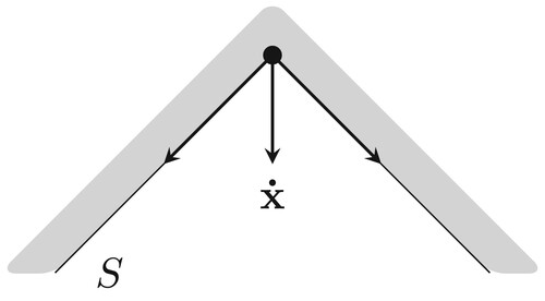
Here, ${\mathbf{v}}_j$ and ${\mathbf{w}}_h$ are vertices of S and $\mathcal{D}$, respectively. l and r are the number of vertices of S and $\mathcal{D}$, respectively. Figure 1 depicts a geometric representation of Theorem 2.3. This theorem states that in order to keep the states in a convex set, the derivative of states at vertices should be pointed inward or lie on the boundaries of the set. In this case, the states cannot go beyond the defined set.

Figure 1. Geometric representation of Theorem 2.3. The arrows indicate the derivative of the states at the vertices of the convex set.

Next theorem extends Theorem 2.3 for the following invariant set. (5) $S=\{{\mathbf{g}}_i^{\mathrm{\top }}\mathbf{x}\le {\theta }_i,{\theta }_i>0,i=1,\dots ,s\},$(5) which S is a compact polyhedron containing the origin and defined by ${\mathbf{g}}_{\mathbf{i}}$ and ${\theta }_i>0$. To do so, the following convex cone is defined. (6) $\begin{array}{rl}{C}_j& =\{{\mathbf{g}}_i^{\mathrm{\top }}\mathbf{x}\le {\theta }_i,{\theta }_i>0,\\ & \mathrm{\forall }{\mathbf{g}}_i^{\mathrm{\top }},{\theta }_i\text{such that}{\mathbf{g}}_i^{\mathrm{\top }}{\mathbf{v}}_j={\theta }_i,{\mathbf{v}}_j\in \mathrm{vert}(S)\}\end{array}$(6)

Theorem 2.4

Blanchini, 1990b

The set defined in (5(5) $S=\{{\mathbf{g}}_i^{\mathrm{\top }}\mathbf{x}\le {\theta }_i,{\theta }_i>0,i=1,\dots ,s\},$(5) ) is invariant for the system (3(3) $\dot{\mathbf{x}}(t)=(A+\mathrm{BKC})\mathbf{x}(t)+E\mathbf{d}(t)=A_{\mathrm{cl}}\mathbf{x}(t)+E\mathbf{d}(t),$(3) ) if and only if there exist a static state feedback K such that (7) $\begin{array}{rl}& {\mathbf{v}}_j+\tau (A_{\mathrm{cl}}{\mathbf{v}}_j+E{\mathbf{w}}_h)\in C_j\\ & \text{for all}\tau >0,{\mathbf{v}}_j\in \mathrm{vert}(S),\mathrm{and}{\mathbf{w}}_h\in \mathrm{vert}(\mathcal{D}),\\ & j=1,\dots ,r,h=1,\dots ,l.\end{array}$(7)

τ is the discretisation time step. The following corollary will restate Theorem 2.4 in an LMI format by shifting the planes of $C_j$ and defining $C_j^{\ast }$ as follows: (8) $\begin{array}{rl}{C}_j^{\ast }& =\{{\mathbf{g}}_i^{\mathrm{\top }}\mathbf{x}\le {\theta }_i-\underset{h}{max}(\tau {\mathbf{g}}_i^{\mathrm{\top }}E{\mathbf{w}}_h),\\ & \mathrm{\forall }{\mathbf{g}}_i^{\mathrm{\top }},{\theta }_i\text{such that}{\mathbf{g}}_i^{\mathrm{\top }}{\mathbf{v}}_j={\theta }_i,{\mathbf{w}}_h\in \mathrm{vert}(\mathcal{D})\}\end{array}$(8)

Corollary 2.5

Blanchini, 1990b

The set (5(5) $S=\{{\mathbf{g}}_i^{\mathrm{\top }}\mathbf{x}\le {\theta }_i,{\theta }_i>0,i=1,\dots ,s\},$(5) ) is PDI for the system (3(3) $\dot{\mathbf{x}}(t)=(A+\mathrm{BKC})\mathbf{x}(t)+E\mathbf{d}(t)=A_{\mathrm{cl}}\mathbf{x}(t)+E\mathbf{d}(t),$(3) ) if and only if for all $\tau >0$, and all ${\mathbf{v}}_j\in \mathrm{vert}(S),j=1,\dots ,r$, there exist a static feedback K such that (9) ${\mathbf{v}}_j+\tau (A_{\mathrm{cl}}{\mathbf{v}}_j)\in C_j^{\ast },\mathrm{\forall }\tau >0,{\mathbf{v}}_j\in \mathrm{vert}(S),j=1,\dots ,r.$(9)

Using this corollary, solving the PDI problem using LMI equations are possible. The following theorem states the conditions of PDI, and it will be used later.

Theorem 2.6

Blanchini, 1990a

Considering S and $\mathcal{D}$ as convex and compact polyhedrons, the closed-loop system (3(3) $\dot{\mathbf{x}}(t)=(A+\mathrm{BKC})\mathbf{x}(t)+E\mathbf{d}(t)=A_{\mathrm{cl}}\mathbf{x}(t)+E\mathbf{d}(t),$(3) ) is PDI if and only if the system is stable, or if the system is marginally stable ($A_{\mathrm{cl}}$ has zero eigenvalues), the marginally stable modes are unreachable modes of $(A_{\mathrm{cl}},E)$.

In other words, this theorem states that if the system has marginally stable modes, the system matrices should be reduced by a linear state transformation as follows to be PDI (10) $(H^{-1}{A}_{\mathrm{cl}}H,H^{-1}E)=(\left[\begin{array}{cc}{A}_{11}& 0\\ 0& A_{22}\end{array}\right],\left[\begin{array}{c}{E}_1\\ 0\end{array}\right]),$(10) which $A_{22}$ eigenvalues are zero, and these states are unreachable by the disturbances.

In the following section, the model of the system is presented, and difficulties of using the mentioned method are presented.

3. System modelling and control difficulties

In this section, the model of the system, and the related properties of the system are presented. According to these properties, it is shown that the mentioned invariant-based control cannot be applied to this system.

3.1. System model

An n bus distribution grid can be described by the following nonlinear load flow equations: (11) $\begin{array}{rl}{\mathbf{P}}_i& =\sum _{j=1}^n|{\mathbf{V}}_i||{\mathbf{V}}_j||Y_{\mathrm{ij}}|\cos ({\theta }_{\mathrm{ij}}-{\omega }_i+{\omega }_j)\end{array}$(11) (12) $\begin{array}{rl}{\mathbf{Q}}_i& =-\sum _{j=1}^n|{\mathbf{V}}_i||{\mathbf{V}}_j||Y_{\mathrm{ij}}|\sin ({\theta }_{\mathrm{ij}}-{\omega }_i+{\omega }_j),\end{array}$(12) which $\mathbf{P}$, $\mathbf{Q}$, $\mathbf{V}$, Y, θ, and $\omega$ 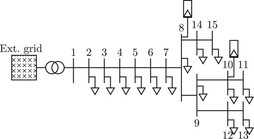are the active power, reactive power, voltage, line admittance, impedance angle, and voltage angle, respectively. The subscript i and ij are related to bus number and the line between bus i and j, respectively. An example of distribution grid is presented in Figure 2. The nonlinear equations can be linearised using the Newton–Raphson method (Saadat, 1999). The discrete linear equations are as follows (13) $\mathbf{V}(k+1)=\mathbf{V}(k)+K_{\mathrm{vp}}\mathrm{\Delta }\mathbf{P}(k)+K_{\mathrm{vq}}\mathrm{\Delta }\mathbf{Q}(k),$(13) which $K_{\mathrm{vp}},K_{\mathrm{vq}}$ are matrices derived from Jacobian matrices, and $\mathrm{\Delta }\mathbf{P}(k)$ and $\mathrm{\Delta }\mathbf{Q}(k)$ are the changes of active and reactive power, that are defined in Wang et al. (2020), Gui et al. (2023), and Hassani et al. (2021). The linearised equations can be stated in continuous form (1(1) $\dot{\mathbf{x}}(t)=A\mathbf{x}(t)+B\mathbf{u}(t)+E\mathbf{d}(t),$(1) ) (Hassani et al., 2023). In this format, the states $\mathbf{x}(t)\in {\mathbb{R}}^n$ would be the deviation of node voltages in per units. The disturbances $\mathbf{d}(t)=\left[\begin{array}{c}\mathbf{p}\\ \mathbf{q}\end{array}\right]$, which $\mathbf{p}\in {\mathbb{R}}^n$ and $\mathbf{q}\in {\mathbb{R}}^n$ are the active and reactive rate of power changes of the nodes. The control inputs $\mathbf{u}\in {\mathbb{R}}^{n_c}$ are the reactive power of the controllable power electronic interfaced devices such as PVs and EVs. $n_c$ is the number of nodes connected to controllable power electronic devices. In the following, N and $N_c$ are defined as the set of all nodes and set of nodes connected to controllable resources, respectively. Elements of $N_c$ are renamed as $l_1,l_2,\dots ,l_{n_c}$. System matrices $A\in {\mathbb{R}}^{n\times n}$, $B\in {\mathbb{R}}^{n\times n_c}$, and $E\in {\mathbb{R}}^{n\times 2n}$ are defined as follows: $\begin{array}{rl}A& =[0{]}_{n\times n},\\ E& =\left[\begin{array}{cccc}{E}_1& E_2& \cdots & E_{2n}\end{array}\right],\\ B& =\left[\begin{array}{ccc}{E}_{n+l_1}& E_{n+l_2}& \dots \end{array}\right],\\ C& =\left[\begin{array}{c}{\mathbf{e}}_{l_1}\\ {\mathbf{e}}_{l_2}\\ ⋮\end{array}\right],\end{array}$which $E_i$ is the ith column of E matrix. The first 14 columns of E are the coefficients for the active power disturbances and the rest are reactive power coefficients. Therefore, B matrix is constructed based on the second 14 column of the E matrix. ${\mathbf{e}}_i$ is a zero vector that the ith element is 1. It is worth mentioning that the A matrix is a null matrix as a result of changing the discrete dynamics to continuous. These equations can be found in Hassani et al. (2023). The local controller have the following form: (14) $K=\mathrm{diag}\{k_{l_1},k_{l_2},\dots \}$(14) $\mathrm{diag}$ is the diagonal format of the elements. K is diagonal since it is a local controller and each bus can only use their own measurements. It is important to understand the structure of $A_{\mathrm{cl}}$ in the low-voltage distribution grid. According to open-loop system matrices presented above, the closed-loop system matrix structure is as follows: (15) $\begin{array}{r}{A}_{\mathrm{cl}}=\left[\begin{array}{ccccccccc}0& \cdots & 0& E_{n+l_1}{k}_{l_1}& 0& E_{n+l_2}{k}_{l_2}& 0& \cdots & 0\end{array}\right].\end{array}$(15) It can be seen that the closed loop system matrix is zero everywhere but the $l_i,i=l_1,l_2,\dots ,l_{n_c}$ columns. As a result, the closed loop matrix have $n-n_c$ zero and $n_c$ non-zero eigenvalues. It is important to mention that the zero eigenvalues are not controllable, while the non-zero ones are controllable. In addition, the non-zero eigenvalues refer to the points that have PVs as controllable generation units.

Figure 2. Fifteen bus reference low-voltage distribution grid belongs to Thy-Mors Energi. Bus number 8 and 10 are equipped with PVs (Gui et al., 2023).

3.2. Control purpose

Having all the voltages of the grid set to the reference is the main goal, but the under-actuated system is not capable of regulating all the voltages to the same reference. Intuitively, this means that the voltages will deviate from the reference at buses where there is no control on the voltages down the grid. Therefore, relaxing the control goal to keeping the voltages within an acceptable range is necessary.

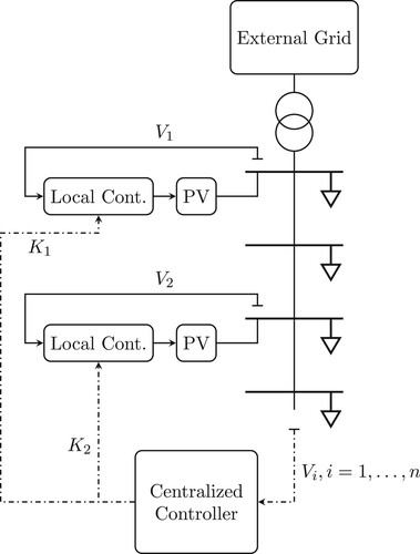
Considering the above paragraph, a centralised controller (CC) is considered in this paper. The control architecture is depicted in Figure 3. In this figure, the local controllers get feedback from their local measurements and generate control inputs for the PV and its power electronic interface. The CC receives measured data from the SMs, and calculates and sends the controller gains to each agent. In other words, the CC tunes the local controllers in this architecture. It is assumed that all the nodes are equipped with SMs. This is a reasonable assumption since for example in Denmark all consumers are equipped with SMs.

Figure 3. Centralised and local control architecture in a low-voltage distribution grid. The flat surface of the lines shows the measurement, and the dash dot lines depict communications.

It is worth mentioning that the centralised control architecture is used in this paper since it is aligned with the existing communication infrastructure in the low-voltage distribution grids. According to Nainar et al. (2021), the SM data are collected using a communication network in the distribution system operator. Therefore, a centralised control unit can be utilised by the distribution system operator, and the control signals can be sent back to the actuators in the grid. In this paper, the distributed control structure has not been discussed, however, applying the invariance-based method to distributed control architecture will be considered as a future research direction.

The centralised feedback loop is a very slow dynamic loop. It means, the SMs sense and store data for large time intervals before sending aggregated values. Assuming that the centralised controller updates its measurements every T seconds, it cannot have active effect during the proceeding T seconds period. Due to the described long intervals T, the CC is designed to tune the local controller at each communication instant.

3.3. Difficulties

Having the above information, some difficulties regarding the invariance control of the system are as follows.

Comparing Theorem 2.6 with the closed-loop system matrices (15(15) $\begin{array}{r}{A}_{\mathrm{cl}}=\left[\begin{array}{ccccccccc}0& \cdots & 0& E_{n+l_1}{k}_{l_1}& 0& E_{n+l_2}{k}_{l_2}& 0& \cdots & 0\end{array}\right].\end{array}$(15) ), it can be seen that $A_{\mathrm{cl}}$ is marginally stable, i.e. that it has zero eigenvalues. These eigenvalues cannot be controlled and moved to the left hand side of the imaginary axis. In addition, all modes of the closed-loop system are reachable, i.e. disturbances in the system affect all the states of the system. Therefore, according to Theorem 2.6, the closed-loop system cannot be PDI.

In the following, two properties of the system are presented. These properties are used in Section 4 for deriving the proposed control method.

• It is necessary to understand the disturbance inputs for the system. Disturbance inputs are rate of power changes. Therefore, the integral of the disturbances during a time period is the sum of the load changes in that period. It should be stated that the load changes in the grid at any time are bounded. Therefore, it is rational to assume that (16) ${\int }_0^t\mathbf{d}(\tau )\mathrm{d}\tau <\mathrm{\infty }.$(16) Therefore, the sum of all the changes of the load can be modelled as $\mathbf{\Gamma }\delta (t)$, which $\mathbf{\Gamma }$ is the sum of all load changes and $\delta (t)$ is the Dirac delta function.

• Sorting the controllable and uncontrollable states as (17) $\mathbf{x}=\left[\begin{array}{c}{\mathbf{x}}_{\mathbf{c}}\\ {\mathbf{x}}_{\mathbf{uc}}\end{array}\right],$(17) system matrices would be as follows: (18) $(\left[\begin{array}{cc}{A}_{11}& 0\\ A_{12}& 0\end{array}\right],\left[\begin{array}{c}{E}_1\\ E_2\end{array}\right]).$(18) Which $E=\left[\begin{array}{c}{E}_1\\ E_2\end{array}\right]$. Reducing these matrices results in (19) $(\left[\begin{array}{cc}{A}_{11}& 0\\ 0& 0\end{array}\right],\left[\begin{array}{c}{E}_1\\ E_2^{\ast }\end{array}\right]).$(19) It is important to mention that in this case $E_2^{\ast }$ will not be zero because E is full rank. Therefore, system states are all reachable.

These two points will lead us to the following method stated in the next section.

4. Proposed method

Sorting the system states into controllable and uncontrollable states gives the following state space equations: (20) $\begin{array}{rl}\dot{\mathbf{x}}& =\left[\begin{array}{c}{\dot{\mathbf{x}}}_{\mathbf{c}}\\ {\dot{\mathbf{x}}}_{\mathbf{uc}}\end{array}\right]=\left[\begin{array}{cc}{A}_{11}& 0\\ A_{12}& A_{\mathrm{uc}}\end{array}\right]\left[\begin{array}{c}{\mathbf{x}}_{\mathbf{c}}\\ {\mathbf{x}}_{\mathbf{uc}}\end{array}\right]+\left[\begin{array}{c}{E}_1\\ E_2\end{array}\right]\mathbf{d},\\ A_{\mathrm{uc}}& =0.\end{array}$(20) The control procedure is divided into controllable and uncontrollable parts in the following two subsections. Afterwards, control input constraints are considered, and finally, an approach to solve and implement equations is presented.

4.1. Uncontrollable states control

According to (20(20) $\begin{array}{rl}\dot{\mathbf{x}}& =\left[\begin{array}{c}{\dot{\mathbf{x}}}_{\mathbf{c}}\\ {\dot{\mathbf{x}}}_{\mathbf{uc}}\end{array}\right]=\left[\begin{array}{cc}{A}_{11}& 0\\ A_{12}& A_{\mathrm{uc}}\end{array}\right]\left[\begin{array}{c}{\mathbf{x}}_{\mathbf{c}}\\ {\mathbf{x}}_{\mathbf{uc}}\end{array}\right]+\left[\begin{array}{c}{E}_1\\ E_2\end{array}\right]\mathbf{d},\\ A_{\mathrm{uc}}& =0.\end{array}$(20) ), the solution of the uncontrollable state space differential equations is as follow: (21) $\begin{array}{r}{\mathbf{x}}_{\mathbf{uc}}(t)={\mathbf{x}}_{\mathbf{uc}}(0)+{\int }_0^t\exp (0(t-\tau ))(A_{12}{\mathbf{x}}_{\mathbf{c}}(\tau )+E_2\mathbf{d}(\tau ))\mathrm{d}\tau .\end{array}$(21) As stated earlier the goal is to keep states in the range $[V_{min},V_{max}]$, hence (22) $\begin{array}{rl}& V_{min}\le \underset{d}{min}\{{\mathbf{x}}_{\mathbf{uc}}(0)+{\int }_0^t(A_{12}{\mathbf{x}}_{\mathbf{c}}+E_2\mathbf{d})\mathrm{d}\tau \},\end{array}$(22) (23) $\begin{array}{rl}& \underset{d}{max}\{{\mathbf{x}}_{\mathbf{uc}}(0)+{\int }_0^t(A_{12}{\mathbf{x}}_{\mathbf{c}}+E_2\mathbf{d})\mathrm{d}\tau \}\le V_{max}.\end{array}$(23) In other words, the minimum of the function should be bigger than $V_{min}$, and the maximum of the function should be smaller than $V_{max}$. These inequalities can be simplified as (24) $\begin{array}{rl}& V_{min}\le \underset{\mathrm{\Gamma }}{min}\{{\mathbf{x}}_{\mathbf{uc}}(0)+(A_{12}{\mathbf{x}}_{\mathbf{I}}+E_2\mathbf{\Gamma })\},\end{array}$(24) (25) $\begin{array}{rl}& \underset{\mathrm{\Gamma }}{max}\{{\mathbf{x}}_{\mathbf{uc}}(0)+(A_{12}{\mathbf{x}}_{\mathbf{I}}+E_2\mathbf{\Gamma })\}\le V_{max}.\end{array}$(25) In these inequalities, $\mathbf{\Gamma }$ is the load changes in the specified interval and it is defined in Section 3.3. In addition $\mathbf{\Gamma }\in \mathcal{D}$, and $\mathcal{D}$ will be defined later. In addition, ${\mathbf{x}}_{\mathbf{I}}={\int }_0^t{\mathbf{x}}_{\mathbf{c}}(\tau )\mathrm{d}\tau$, and $A_{12}{\mathbf{x}}_{\mathbf{I}}$ shows the contribution of the controllable states to the uncontrollable states. This can be stated in the following way. The controllable states can help the uncontrollable states to remain in the specified limits stated in Equations (24(24) $\begin{array}{rl}& V_{min}\le \underset{\mathrm{\Gamma }}{min}\{{\mathbf{x}}_{\mathbf{uc}}(0)+(A_{12}{\mathbf{x}}_{\mathbf{I}}+E_2\mathbf{\Gamma })\},\end{array}$(24) ) and (25(25) $\begin{array}{rl}& \underset{\mathrm{\Gamma }}{max}\{{\mathbf{x}}_{\mathbf{uc}}(0)+(A_{12}{\mathbf{x}}_{\mathbf{I}}+E_2\mathbf{\Gamma })\}\le V_{max}.\end{array}$(25) ). It is important to mention that $A_{12}$ contains the controller.

Equations (24(24) $\begin{array}{rl}& V_{min}\le \underset{\mathrm{\Gamma }}{min}\{{\mathbf{x}}_{\mathbf{uc}}(0)+(A_{12}{\mathbf{x}}_{\mathbf{I}}+E_2\mathbf{\Gamma })\},\end{array}$(24) ) and (25(25) $\begin{array}{rl}& \underset{\mathrm{\Gamma }}{max}\{{\mathbf{x}}_{\mathbf{uc}}(0)+(A_{12}{\mathbf{x}}_{\mathbf{I}}+E_2\mathbf{\Gamma })\}\le V_{max}.\end{array}$(25) ) present two inequalities, and in order to preserve them, $A_{12}{\mathbf{x}}_{\mathbf{I}}$ can be tuned. Since $A_{12}{\mathbf{x}}_{\mathbf{I}}$ consists of the control gain, achieving these inequalities is possible.

4.2. Controllable states control

According to Theorem 2.6, invariant-based control stated in Corollary 2.5 can be applied to the controllable state space model (20(20) $\begin{array}{rl}\dot{\mathbf{x}}& =\left[\begin{array}{c}{\dot{\mathbf{x}}}_{\mathbf{c}}\\ {\dot{\mathbf{x}}}_{\mathbf{uc}}\end{array}\right]=\left[\begin{array}{cc}{A}_{11}& 0\\ A_{12}& A_{\mathrm{uc}}\end{array}\right]\left[\begin{array}{c}{\mathbf{x}}_{\mathbf{c}}\\ {\mathbf{x}}_{\mathbf{uc}}\end{array}\right]+\left[\begin{array}{c}{E}_1\\ E_2\end{array}\right]\mathbf{d},\\ A_{\mathrm{uc}}& =0.\end{array}$(20) ). To do so, the set S is defined as (26) $S=\{x_i\in {\mathbf{x}}_{\mathbf{c}}|-\alpha \le x_i\le \alpha \}.$(26) This set can be written as a polyhedron in Equation (5(5) $S=\{{\mathbf{g}}_i^{\mathrm{\top }}\mathbf{x}\le {\theta }_i,{\theta }_i>0,i=1,\dots ,s\},$(5) ). An example is presented in the Section 6. It is assumed that disturbances are limited as follows (27) $d_{min}\le d_i\le d_{max},i=1,\dots ,n.$(27) Therefore, $\mathcal{D}\subset {\mathbb{R}}^{n\times 1}$ has $d_i$ as dimensions. The vertices of $\mathbb{D}$ is defined as ${\mathbf{w}}_h,h=1,\dots ,l$. According to Corollary 2.5, the closed-loop system is invariant if and only if there is a feedback K such that the following inequalities hold. (28) $\begin{array}{rl}& {\mathbf{g}}_i^{\mathrm{\top }}({\mathbf{v}}_j+\tau (A_{\mathrm{cl}}{\mathbf{v}}_j))\le {\theta }_i-\underset{h}{max}(\tau {\mathbf{g}}_i^{\mathrm{\top }}E{\mathbf{w}}_h)\\ & \mathrm{\forall }{\mathbf{g}}_i^{\mathrm{\top }},{\theta }_i\text{such that}{\mathbf{g}}_i^{\mathrm{\top }}{\mathbf{v}}_j={\theta }_i,{\mathbf{w}}_h\in \mathrm{vert}(\mathcal{D}).\end{array}$(28)

4.3. Control input constraints

Due to limitations in PVs and power electronic devices, and also reactive power injection effects the control inputs are constraint. This constraint is mentioned in (2(2) $\mathbf{x}(t)\in \mathcal{X},\mathbf{u}(t)\in \mathcal{U},\mathbf{d}(t)\in \mathcal{D},$(2) ) as $\mathbf{u}(t)\in \mathcal{U}$. Since $\mathbf{u}(t)=K{\mathbf{x}}_{\mathbf{c}}$, it is enough to evaluate the constraint on the vertices of the invariant set S for the controllable states, since this is the worst possible case. In other words, (29) $K{\mathbf{v}}_i\in \mathcal{U},i=1,2,3,4.$(29) This can be used to capture the reactive power limitations in case of low power generation caused by low solar irradiation.

4.4. Control structure

According to previous two sections, Equation (28(28) $\begin{array}{rl}& {\mathbf{g}}_i^{\mathrm{\top }}({\mathbf{v}}_j+\tau (A_{\mathrm{cl}}{\mathbf{v}}_j))\le {\theta }_i-\underset{h}{max}(\tau {\mathbf{g}}_i^{\mathrm{\top }}E{\mathbf{w}}_h)\\ & \mathrm{\forall }{\mathbf{g}}_i^{\mathrm{\top }},{\theta }_i\text{such that}{\mathbf{g}}_i^{\mathrm{\top }}{\mathbf{v}}_j={\theta }_i,{\mathbf{w}}_h\in \mathrm{vert}(\mathcal{D}).\end{array}$(28) ) keep the states in the defined S set, and Equations (24(24) $\begin{array}{rl}& V_{min}\le \underset{\mathrm{\Gamma }}{min}\{{\mathbf{x}}_{\mathbf{uc}}(0)+(A_{12}{\mathbf{x}}_{\mathbf{I}}+E_2\mathbf{\Gamma })\},\end{array}$(24) )–(25(25) $\begin{array}{rl}& \underset{\mathrm{\Gamma }}{max}\{{\mathbf{x}}_{\mathbf{uc}}(0)+(A_{12}{\mathbf{x}}_{\mathbf{I}}+E_2\mathbf{\Gamma })\}\le V_{max}.\end{array}$(25) ) are keeping the uncontrollable states in the desired set. Therefore, solving these equations will keep all the states in the desired range. The result of solving these inequalities will be local control feedback. This solution can be further limited by considering the control input constraints in Equation (29(29) $K{\mathbf{v}}_i\in \mathcal{U},i=1,2,3,4.$(29) ).

It can be seen that Equations (24(24) $\begin{array}{rl}& V_{min}\le \underset{\mathrm{\Gamma }}{min}\{{\mathbf{x}}_{\mathbf{uc}}(0)+(A_{12}{\mathbf{x}}_{\mathbf{I}}+E_2\mathbf{\Gamma })\},\end{array}$(24) )–(25(25) $\begin{array}{rl}& \underset{\mathrm{\Gamma }}{max}\{{\mathbf{x}}_{\mathbf{uc}}(0)+(A_{12}{\mathbf{x}}_{\mathbf{I}}+E_2\mathbf{\Gamma })\}\le V_{max}.\end{array}$(25) ) depends on both ${\mathbf{x}}_{\mathbf{I}}$ and K, but it is not necessary to evaluate the inequalities on all ${\mathbf{x}}_{\mathbf{I}}$. Evaluating the inequalities on the worst points, which are the vertices of the polyhedron S will give the worst conditions. In other words, ${\mathbf{x}}_{\mathbf{I}}$ is in convex hull of ${\mathbf{v}}_j$. Hence, uncontrollable states inequalities would be: (30) $\begin{array}{rl}& V_{min}\le \underset{\mathrm{\Gamma }}{min}\{{\mathbf{x}}_{\mathbf{uc}}(0)+(A_{12}{\mathbf{v}}_j+E_2\mathbf{\Gamma })\},\end{array}$(30) (31) $\begin{array}{rl}& \underset{\mathrm{\Gamma }}{max}\{{\mathbf{x}}_{\mathbf{uc}}(0)+(A_{12}{\mathbf{v}}_j+E_2\mathbf{\Gamma })\}\le V_{max}.\\ & \mathrm{\forall }j=1,\dots ,4,\mathrm{\Gamma }\in {\mathbf{w}}_h,\end{array}$(31) Considering a specified set (26(26) $S=\{x_i\in {\mathbf{x}}_{\mathbf{c}}|-\alpha \le x_i\le \alpha \}.$(26) ) for the controllable states may cause the uncontrollable states inequalities (30(30) $\begin{array}{rl}& V_{min}\le \underset{\mathrm{\Gamma }}{min}\{{\mathbf{x}}_{\mathbf{uc}}(0)+(A_{12}{\mathbf{v}}_j+E_2\mathbf{\Gamma })\},\end{array}$(30) )–(31(31) $\begin{array}{rl}& \underset{\mathrm{\Gamma }}{max}\{{\mathbf{x}}_{\mathbf{uc}}(0)+(A_{12}{\mathbf{v}}_j+E_2\mathbf{\Gamma })\}\le V_{max}.\\ & \mathrm{\forall }j=1,\dots ,4,\mathrm{\Gamma }\in {\mathbf{w}}_h,\end{array}$(31) ) be infeasible. In order to make sure that the uncontrollable inequalities are feasible, more restricted set for controllable sets should be considered. In other words, by limiting the controllable states to tighter sets, the uncontrollable states cannot exceed the limits, since the uncontrollable states are affected by the controllable states directly. Therefore, it is desirable to consider the set S or its vertices ${\mathbf{v}}_j$ as variables. However, this consideration make Equations (30(30) $\begin{array}{rl}& V_{min}\le \underset{\mathrm{\Gamma }}{min}\{{\mathbf{x}}_{\mathbf{uc}}(0)+(A_{12}{\mathbf{v}}_j+E_2\mathbf{\Gamma })\},\end{array}$(30) )–(31(31) $\begin{array}{rl}& \underset{\mathrm{\Gamma }}{max}\{{\mathbf{x}}_{\mathbf{uc}}(0)+(A_{12}{\mathbf{v}}_j+E_2\mathbf{\Gamma })\}\le V_{max}.\\ & \mathrm{\forall }j=1,\dots ,4,\mathrm{\Gamma }\in {\mathbf{w}}_h,\end{array}$(31) ) non-convex.

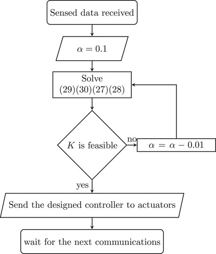
In order to solve the problem mentioned above, the flow chart in Figure 4 is proposed for the control structure. In this diagram, the biggest possible set is chosen for the algorithm. Feasibility of equations will decide on the rest of the algorithm, i.e. if the equations are feasible, we are satisfied. If equations are not feasible, tighter sets will be chosen for the controllable states.

Figure 4. Flow chart of the centralised control process. The process starts with receiving data in the CC until sending the local controller coefficients.

The next section, presents a hybrid model for the distribution grid and analyse the control algorithm in a hybrid framework.

5. Hybrid modelling & control

As stated above, the centralised control loop has a very slow discrete dynamics. On the other hand, the electrical grid has a continuous dynamics. The combination of the communications and electrical subsystems can also be interpreted as cyber-physical system. In Hassani et al. (2023), a hybrid model is presented in order to consider the continuous and discrete dynamics of the system together. The hybrid system states are the voltage deviation states stated previously in this paper $\mathbf{x}$ augmented with a timer state τ and CC states ${\mathbf{u}}_{\mathbf{c}}$ as ${\mathbf{x}}_{\mathcal{H}}=\left[\begin{array}{c}\mathbf{x}\\ {\mathbf{u}}_{\mathbf{c}}\\ \tau \end{array}\right].$The hybrid dynamics can be stated as: (32) $\begin{array}{r}\{\begin{array}{l}{\dot{\mathbf{x}}}_{\mathcal{H}}=f({\mathbf{x}}_{\mathcal{H}})=\left[\begin{array}{c}\dot{\mathbf{x}}\\ 0\\ 1\end{array}\right],\zeta =({\mathbb{R}}^n\times {\mathbb{R}}^{n_c}\times [0,T])\\ {\mathbf{x}}_{\mathcal{H}}^{+}=g({\mathbf{x}}_{\mathcal{H}})=\left[\begin{array}{c}\mathbf{x}\\ \kappa \mathbf{(}\mathbf{x}\mathbf{)}\\ 0\end{array}\right],\mathrm{\Lambda }=({\mathbb{R}}^n\times {\mathbb{R}}^{n_c}\times \{T\})\end{array},\end{array}$(32) in which f and g are the flow map and jump map of the hybrid systems, and ζ and Λ are the flow set and jump set of the system. The flow map is active in the flow set, which the time states are limited to the set $[0,T]$. If the timer state exceeds the set ζ a jump will happen in the system, meaning that the SMs send the data to the centralised controller and will be delivered to the actuators of the system. The hybrid model was first introduced in Hassani et al. (2021).

In this section, the hybrid model is used to evaluate the effect of the jumps in the system; accordingly, the following paragraphs analyse the invariance of the system for the flow and jump map.

In order to show the system is invariant for the hybrid case, it is necessary to consider a general invariant set for all of the states, i.e. that a set should be defined that all the states at any time should remain in that set. To do so, $10\mathrm{\%}$ deviation is considered for the voltages of the system as (33) $S^{\ast }=\{\mathbf{x}\in {\mathbb{R}}^n|-0.1\le x_i\le 0.1,i=1,\dots ,n\}.$(33) In Section 4, the control method guarantees that the states of the system will remain in $S^{\ast }$ since the set S is a subset of $S^{\ast }$.

According to the hybrid model (32(32) $\begin{array}{r}\{\begin{array}{l}{\dot{\mathbf{x}}}_{\mathcal{H}}=f({\mathbf{x}}_{\mathcal{H}})=\left[\begin{array}{c}\dot{\mathbf{x}}\\ 0\\ 1\end{array}\right],\zeta =({\mathbb{R}}^n\times {\mathbb{R}}^{n_c}\times [0,T])\\ {\mathbf{x}}_{\mathcal{H}}^{+}=g({\mathbf{x}}_{\mathcal{H}})=\left[\begin{array}{c}\mathbf{x}\\ \kappa \mathbf{(}\mathbf{x}\mathbf{)}\\ 0\end{array}\right],\mathrm{\Lambda }=({\mathbb{R}}^n\times {\mathbb{R}}^{n_c}\times \{T\})\end{array},\end{array}$(32) ), during the jumps, states will not change during the jumps. Since states are in $S^{\ast }$ during the flows, they will remain in $S^{\ast }$ at jumps.

It is important to analyse the effects of the CC state on the system. During the jumps the CC changes its value, but it will not affect the states at the jumps. Assuming a jump happens at T, the CC generates the local controller gains based on $\mathbf{x}(T)$, and will be applied to $[T,2T]$. Therefore, the local controllers rely on a feedback which is designed or the same time instant.

It can be concluded that the states of the system (Voltages) will remain in the desired set. However, the feedback loop is based on ideal communications, and delay is not considered in the hybrid model. The hybrid model (32(32) $\begin{array}{r}\{\begin{array}{l}{\dot{\mathbf{x}}}_{\mathcal{H}}=f({\mathbf{x}}_{\mathcal{H}})=\left[\begin{array}{c}\dot{\mathbf{x}}\\ 0\\ 1\end{array}\right],\zeta =({\mathbb{R}}^n\times {\mathbb{R}}^{n_c}\times [0,T])\\ {\mathbf{x}}_{\mathcal{H}}^{+}=g({\mathbf{x}}_{\mathcal{H}})=\left[\begin{array}{c}\mathbf{x}\\ \kappa \mathbf{(}\mathbf{x}\mathbf{)}\\ 0\end{array}\right],\mathrm{\Lambda }=({\mathbb{R}}^n\times {\mathbb{R}}^{n_c}\times \{T\})\end{array},\end{array}$(32) ) is extended to consider delay in Hassani et al. (2023). Considering the delayed hybrid model adds additional constraints to the method, which will not be addressed explicitly here.

Remark 5.1

To elaborate, the time diagram of the communication structure of the low-voltage distribution grids is depicted in Figure 5. The SMs collect data for T seconds and send it to the CC, and CC sends the controller gains to the PVs. It should be mentioned that the process has both communication delay and processing delay. It can be seen that the controller at time $T_d$ uses data sampled at time zero, i.e. there is mismatch between the data used for controller design and real state of the system at time $T_d$.

Figure 5. The CC uses the data at time 0 to design the controller coefficients, however it will applied at time $0+T_d$. Therefore, the design should compensate for the changes during $T_d$ seconds. On the other hand, the previous method is designed to consider T second intervals. However, in this structure, the design should consider $[0,T+T_d]$ interval.

Therefore, the designed controller should consider the mismatch caused by the delay and also it has to work for the period of $[T_{d1},T+T_{d2}]$. The inequalities (30(30) $\begin{array}{rl}& V_{min}\le \underset{\mathrm{\Gamma }}{min}\{{\mathbf{x}}_{\mathbf{uc}}(0)+(A_{12}{\mathbf{v}}_j+E_2\mathbf{\Gamma })\},\end{array}$(30) ) and (31(31) $\begin{array}{rl}& \underset{\mathrm{\Gamma }}{max}\{{\mathbf{x}}_{\mathbf{uc}}(0)+(A_{12}{\mathbf{v}}_j+E_2\mathbf{\Gamma })\}\le V_{max}.\\ & \mathrm{\forall }j=1,\dots ,4,\mathrm{\Gamma }\in {\mathbf{w}}_h,\end{array}$(31) ) for the first communication will become as follows: (34) $\begin{array}{rl}& V_{min}\le \underset{\mathbf{\Gamma },\mathrm{\Delta }{\mathbf{x}}_{\mathbf{uc}}}{min}\{({\mathbf{x}}_{\mathbf{uc}}(0)+\mathrm{\Delta }{\mathbf{x}}_{\mathbf{uc}})+(A_{12}{\mathbf{v}}_j+E_2\mathbf{\Gamma })\},\end{array}$(34) (35) $\begin{array}{rl}& \underset{\mathbf{\Gamma },\mathrm{\Delta }{\mathbf{x}}_{\mathbf{uc}}}{max}\{({\mathbf{x}}_{\mathbf{uc}}(0)+\mathrm{\Delta }{\mathbf{x}}_{\mathbf{uc}})+(A_{12}{\mathbf{v}}_j+E_2\mathbf{\Gamma })\}\le V_{max}.\\ & \mathrm{\forall }j=1,\dots ,4,\mathbf{\Gamma }\in {\mathbf{w}}_h,\end{array}$(35) where $\mathrm{\Delta }{\mathbf{x}}_{\mathbf{uc}}$ is the changes of the states from the sensing points at $0,T,2T,\dots$ and the applying points at $0+T_d,T+T_d,2T+T_d,\dots$. It should be mentioned that Equations (28(28) $\begin{array}{rl}& {\mathbf{g}}_i^{\mathrm{\top }}({\mathbf{v}}_j+\tau (A_{\mathrm{cl}}{\mathbf{v}}_j))\le {\theta }_i-\underset{h}{max}(\tau {\mathbf{g}}_i^{\mathrm{\top }}E{\mathbf{w}}_h)\\ & \mathrm{\forall }{\mathbf{g}}_i^{\mathrm{\top }},{\theta }_i\text{such that}{\mathbf{g}}_i^{\mathrm{\top }}{\mathbf{v}}_j={\theta }_i,{\mathbf{w}}_h\in \mathrm{vert}(\mathcal{D}).\end{array}$(28) ) and (29(29) $K{\mathbf{v}}_i\in \mathcal{U},i=1,2,3,4.$(29) ) will not change in this situation.

However, the above equations rely on the knowledge of the voltage mismatch caused by the delay. Assuming bounds on the changes of voltage (mismatch) during delay are known, the above problem is solvable. However, this cannot always be assumed and we leave this aspect open for future research.

6. Case studies

In this section, numerical examples and case studies are presented to show the method feasibility and effectiveness. In this paper, the 15 bus low-voltage distribution grid presented in Figure 2 is considered as the case study. The low-voltage grid is connected through a 10/0.4 kVA transformer to the medium-voltage grid. The grid operates on 50 Hz frequency. π-model is used for representing the electrical cables, and P-Q load model is used for loads and generators. The connected PVs are rates at 5 kVA. The irradiation (consequently, active power generation) has been considered constant in this paper. However, by considering non-constant active power generation, the considered disturbance level of the grid may change. This can be done by reevaluating the possible load changes (disturbances) in the grid.

Additionally, 15 min update interval is selected according to SM and communication network limitations in the low-voltage distribution grids. According to Nainar et al. (2021) and Kemal et al. (2020), SMs collect data for 15 min time intervals and communicate data with the distribution system operator every 6 h. However, it is expected that SMs can communicate in 15 min time interval, as it is considered widely in the literature as well.

The following section presents the feasible sets of the system in a special case. Subsection 6.2 presents an example to illustrate the method. Finally, the effectiveness of the method is illustrated in Section 6.3.

Figure 2 represents the low-voltage distribution grid, and it is assumed that bus number 8 and 10 are controllable; therefore, controllable states and state space would be (36) $\begin{array}{rl}{\mathbf{x}}_{\mathbf{c}}& ={\left[\begin{array}{cc}{x}_8& x_{10}\end{array}\right]}^{\mathrm{\top }}\end{array}$(36) (37) $\begin{array}{rl}{\dot{\mathbf{x}}}_{\mathbf{c}}& =A_{11}{\mathbf{x}}_{\mathbf{c}}+E_1\mathbf{d},\end{array}$(37) related matrix would be (38) $A_{11}=\left[\begin{array}{cc}{a}_{8,8}& a_{8,10}\\ a_{10,8}& a_{10,10}\end{array}\right],$(38) in which $a_{i,j}$s are the elements of the $A_{\mathrm{cl}}$ matrix.

The uncontrollable states are all the states but $x_8$ and $x_{10}$. The state space of these states are as follows: (39) ${\dot{\mathbf{x}}}_{\mathbf{uc}}=A_{\mathrm{uc}}{\mathbf{x}}_{\mathbf{uc}}+A_{12}\left[\begin{array}{c}{x}_8\\ x_{10}\end{array}\right]+E_2\mathbf{d}.$(39) Related matrices would be (40) $\begin{array}{rl}{A}_{\mathrm{uc}}& =0_{12\times 12},\end{array}$(40) (41) $\begin{array}{rl}{A}_{12}& =\left[\begin{array}{cc}{a}_{1,8}& a_{1,10}\\ ⋮& ⋮\\ a_{7,8}& a_{7,10}\\ a_{9,8}& a_{9,10}\\ a_{11,8}& a_{11,10}\\ ⋮& ⋮\\ a_{14,8}& a_{14,10}\end{array}\right].\end{array}$(41) For this system, the S set is defined as follows: (42) $S=\{\left[\begin{array}{c}{x}_8\\ x_{10}\end{array}\right]|-\alpha \le x_8,x_{10}\le \alpha \}.$(42) Rewriting S in the format in Equation (5(5) $S=\{{\mathbf{g}}_i^{\mathrm{\top }}\mathbf{x}\le {\theta }_i,{\theta }_i>0,i=1,\dots ,s\},$(5) ) results in the following ${\mathbf{g}}_i$ and ${\theta }_i$: $\begin{array}{rl}{\mathbf{g}}_1& =\left[\begin{array}{c}1\\ 0\end{array}\right],{\mathbf{g}}_2=\left[\begin{array}{c}0\\ 1\end{array}\right],{\mathbf{g}}_3=\left[\begin{array}{c}-1\\ 0\end{array}\right],{\mathbf{g}}_4=\left[\begin{array}{c}0\\ -1\end{array}\right]\\ {\theta }_i& =\alpha ,\mathrm{\forall }i=1,\dots ,4.\end{array}$Vertices of S (${\mathbf{v}}_j$) would be (43) ${\mathbf{v}}_j\in \{\alpha \left[\begin{array}{c}1\\ 1\end{array}\right],\alpha \left[\begin{array}{c}-1\\ 1\end{array}\right],\alpha \left[\begin{array}{c}1\\ -1\end{array}\right],\alpha \left[\begin{array}{c}-1\\ -1\end{array}\right]\}.$(43) In this case, α is a positive number less or equal to 0.1. It is assumed that disturbances are limited as follows: (44) $d_{min}\le d_i\le d_{max},i=1,\dots ,14.$(44)

6.1. Feasible points

In this part, feasible solutions of the problem for a special case is presented. Feasible sets for different constraints of the method is depicted, and the intersection of them as the feasible set is discussed.

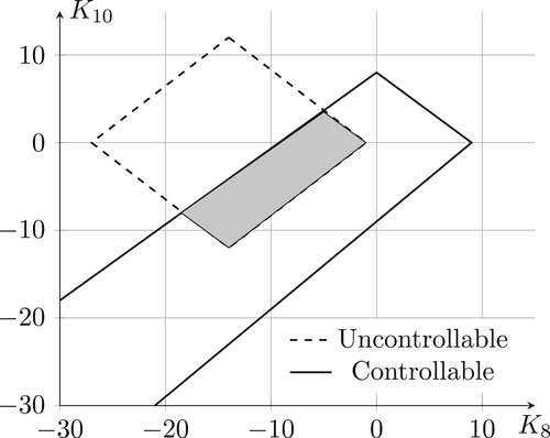
Figure 6 presents feasible points of the algorithm. In this figure, uncontrollable state inequalities (30(30) $\begin{array}{rl}& V_{min}\le \underset{\mathrm{\Gamma }}{min}\{{\mathbf{x}}_{\mathbf{uc}}(0)+(A_{12}{\mathbf{v}}_j+E_2\mathbf{\Gamma })\},\end{array}$(30) )–(31(31) $\begin{array}{rl}& \underset{\mathrm{\Gamma }}{max}\{{\mathbf{x}}_{\mathbf{uc}}(0)+(A_{12}{\mathbf{v}}_j+E_2\mathbf{\Gamma })\}\le V_{max}.\\ & \mathrm{\forall }j=1,\dots ,4,\mathrm{\Gamma }\in {\mathbf{w}}_h,\end{array}$(31) ) results in the feasible points showed by the dashed contour. Feasible points of controllable inequality (28(28) $\begin{array}{rl}& {\mathbf{g}}_i^{\mathrm{\top }}({\mathbf{v}}_j+\tau (A_{\mathrm{cl}}{\mathbf{v}}_j))\le {\theta }_i-\underset{h}{max}(\tau {\mathbf{g}}_i^{\mathrm{\top }}E{\mathbf{w}}_h)\\ & \mathrm{\forall }{\mathbf{g}}_i^{\mathrm{\top }},{\theta }_i\text{such that}{\mathbf{g}}_i^{\mathrm{\top }}{\mathbf{v}}_j={\theta }_i,{\mathbf{w}}_h\in \mathrm{vert}(\mathcal{D}).\end{array}$(28) ) is also shown in the Figure. Finally, the intersection of the two sets are presented by the highlighted region. It should be stated that this region also contains positive controller gains. Since positive gains drive the eigenvalues of the system to instability, the positive gains will not be considered.

In this case, the disturbance set is considered as $-400\le d_i\le 400\mathrm{Watts}/\mathrm{Var},i=1,\dots ,14$ per 15 min. Disturbances are selected according to the historical data of load changes. The disturbance range is considered higher than average power changes of the nodes. The low-voltage distribution grid data are presented in Iov and Ciontea (2021). $\alpha =0.1$ and the following initial values in per unit ($p.u.$) for the states are considered. $\begin{array}{rl}x(0)& =[1,0.99,0.99,0.99,0.98,0.97,0.97,0.96,0.96\\ & 0.95,0.95,0.96,0.96,0.96,0.96].\end{array}$

Figure 6. Feasible sets of controller gains from controllable and uncontrollable states conditions. The grey area is the intersection of the two sets, and feasible set of the problem.

6.2. Case 1

In this part, the procedure of the algorithm is depicted.

The model in Section 5 has been used for simulations and are done in HyEq toolbox (Sanfelice et al., 2013), which is a toolbox for hybrid systems simulations. The mentioned toolbox is used since the system dynamics are hybrid and also, the effectiveness of the control approach can be completely described since it considers the hybrid nature of the system.

In this case, the CC update the control references every 15 min ($T=15min$). This interval has been considered according to the disturbance set $w_h$ considered to be $\pm 500\mathrm{Watts}/\mathrm{Var}$ for every node per 15 min. α is set to $0.1p.u.$ for all the states, meaning that the voltages are allowed to vary in the set $[0.91.1]p.u$ considering the defined disturbances.

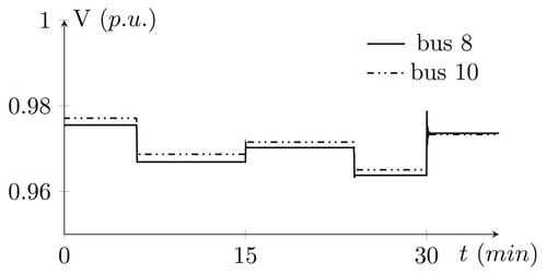
It is assumed that a load disturbance enters the system at the 6 min of simulations. Due to the communication restrictions, the CC cannot respond to the disturbance until the CC update the local gains at 15 min. Voltage profiles of bus 8 and 10 are depicted in Figure 7. At 24 min of the simulation another load change enters the system, and the CC update the local controller coefficients since the previous values were not able to compensate for the voltage drop.

Figure 7. Voltage of the 8^th and 10^th bus.

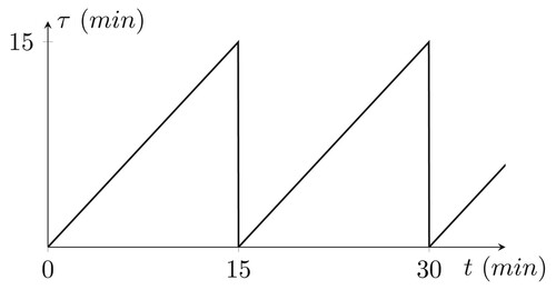
In order to understand the jump and flow of the system, Figure 8 is presented. During the flow (continuous part of the model), the timer state counts from 0 to 15 min, and at the jumps, the timer state resets to zero.

Figure 8. Timer state of the hybrid system.

It is important to understand that despite the disturbance in the system, the designed controllers before the first jump and after the first jump, are able to restrict the voltages in the desired range. This will be further discussed and compared with real scenarios in the next scenario.

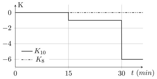
Finally, the local controller coefficients which are tuned by the CC are previewed in Figure 9. These values are updated in the jumps, or in other words, when the communications happen in the system.

Figure 9. Local control coefficients tuned by the CC.

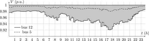
6.3. Case 2

In this scenario, a 24 h simulation is presented. The SMs recorded the mean values of active and reactive load consumption in 15 min intervals (Iov & Ciontea, 2021). Disturbance invariant sets are set to $\pm 400\mathrm{Watts}$ for each node. It is worth mentioning that although this disturbance looks small for a single node, but since the method considers maximum and minimum for all the nodes at the same time, it is enough for the considered grid.

Figure 10 presents voltage profile for bus 12 and 5. It can be seen that the voltage magnitude does not exceed the invariant set. The voltage profiles for all the nodes of the grid are also lie in the grey area depicted in Figure 10. As an example 5th bus voltage profile is shown in the grey area.

Figure 10. Voltage of the bus number 7 and 15. The grey area is the varying region of the voltages of all nodes. The upper limit for the voltages is the first bus which is almost constant.

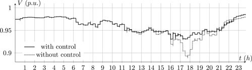
The local controller coefficients are depicted in Figure 11. The coefficients are updated every 15 min. At the start of simulations, the coefficients are zero since voltage deviations are low. On the other hand, during peak consumption of the day, when the voltages start to drop, the effects of the control method start to increase. Finally, control effort goes to zero at the end of simulation. Comparing 10th bus voltage profile in the controlled and not controlled modes show the effectiveness of the method. This comparison is depicted in Figure 12.

Figure 11. Local Controller coefficients updated by the CC.

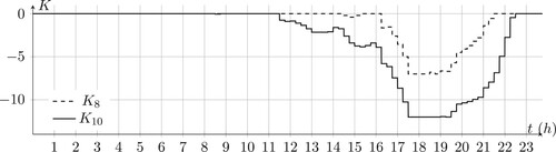
Figure 12. Comparison of bus 10 Voltage in the presence of invariant-based control with no-control case.

7. Discussion

In this section, a discussion of the presented method and the contributions are stated.

The necessity of communication-based voltage control for low-voltage distribution grids has been discussed previously in Bolognani et al. (2019). Additionally, the existing infrastructure facilitates the use of a centralised control structure. Additionally, due to the vast geographical region of low-voltage grids and high number of consumers, the communication has some short comes, such as big update intervals and delays. On the physical (electrical) layer, it cannot be assumed that all the consumers use controllable power electronic devices (PV specifically). As a consequence, the grid will not be fully controllable, which results in the reachability difficulty stated previously.

The proposed method considers the physical burdens as well as the communication burdens in the design procedure, and therefore, guarantees compliance with grid codes. Despite the vast literature, previous methods did not address the mentioned problems together, and more accurately, did not present guarantees on the performance of the method in the presence of the above problems. Additionally, the invariance-based method presented here is able to cope with the reachability issues present in the system set-up considered, which earlier methods could not.

It is acknowledged that the problem of the delay in the design process is not fully addressed in this paper, and this is seen as a future research topic. Additionally, the presented method can be expanded to consider power curtailment for voltage control in cases where reactive power is insufficient for compensation. This is also considered as a future research topic.

8. Conclusion

This paper presents an invariance-based control approach for managing voltage levels within centralised control architectures of low-voltage distribution grids. The conventional invariance-based methods prove unsuitable for the studied system due to reachability of the disturbances to the uncontrollable states. Therefore, an input–output stability method is presented to complement the invariance-based method.

Furthermore, a hybrid model is employed to verify the invariance of the system in the presence of communication deficiencies. It is proved that the voltages can stay at the desired intervals despite the long update intervals of the communications. In other words, long update intervals, CCs can contribute to the local controllers and the voltage profile as a result. In addition, the hybrid model is shown to be effective in analysing the continuous and discrete dynamics of the system. The hybrid model helps in implementing the system due to the availability of hybrid simulators.

Although long update interval as a communication non-ideality is addressed in this paper, communication delay is yet to be considered, and it will be considered in future works.

Disclosure statement

No potential conflict of interest was reported by the author(s).

References

- Blanchini, F. (1990a). Constrained control for perturbed linear systems [Conference session]. 29th IEEE Conference on Decision and Control, Honolulu, HI, USA (pp. 3464–3467, Vol. 6). https://doi.org/10.1109/CDC.1990.203446
- Blanchini, F. (1990b). Feedback control for linear time-invariant systems with state and control bounds in the presence of disturbances. IEEE Transactions on Automatic Control, 35(11), 1231–1234. https://doi.org/10.1109/9.59808
- Bolognani, S., Carli, R., Cavraro, G., & Zampieri, S. (2019). On the need for communication for voltage regulation of power distribution grids. IEEE Transactions on Control of Network Systems, 6(3), 1111–1123. https://doi.org/10.1109/tcns.2019.2921268
- Chong, M. S., Umsonst, D., & Sandberg, H. (2019a). Local voltage control of an inverter-based power distribution network with a class of slope-restricted droop controllers. IFAC-PapersOnLine, 52(20), 163–168. https://doi.org/10.1016/j.ifacol.2019.12.152
- Chong, M. S., Umsonst, D., & Sandberg, H. (2019b). Voltage regulation of a power distribution network in a radial configuration with a class of sector-bounded droop controllers. In 2019 IEEE 58th Conference on Decision and Control (CDC). IEEE. https://doi.org/10.1109/cdc40024.2019.9029681
- Dall'Anese, E., Dhople, S. V., & Giannakis, G. B. (2014). Optimal dispatch of photovoltaic inverters in residential distribution systems. IEEE Transactions on Sustainable Energy, 5(2), 487–497. https://doi.org/10.1109/tste.2013.2292828
- Goebel, R., Sanfelice, R. G., & Teel, A. R. (2009). Hybrid dynamical systems. IEEE Control Systems, 29(2), 28–93. https://doi.org/10.1109/mcs.2008.931718
- Goebel, R., Sanfelice, R. G., & Teel, A. R. (2012). Hybrid dynamical systems: Modeling, stability, and robustness. Princeton University Press. http://www.jstor.org/stable/j.ctt7s02z.
- Gui, Y., Nainar, K., Ciontea, C. I., Bendtsen, J. D., Iov, F., Shahid, K., & Stoustrup, J. (2023). Automatic voltage regulation application for PV inverters in low-voltage distribution grids – A digital twin approach. International Journal of Electrical Power & Energy Systems, 149, Article 109022. https://doi.org/10.1016/j.ijepes.2023.109022
- Hassani, S., Bendtsen, J. D., & Olsen, R. L. (2021). Hybrid modeling of cyber-physical distribution grids. In 2021 IEEE International Conference on Communications, Control, and Computing Technologies for Smart Grids (SmartGridComm). IEEE. https://doi.org/10.1109/smartgridcomm51999.2021.9632321
- Hassani, S., Olsen, R. L., & Bendtsen, J. D. (2023). A hybrid approach to modeling of cyber-physical distribution grids considering packet losses & delays [Conference session]. IECON 2023—49th Annual Conference of the IEEE Industrial Electronics Society, Singapore, Singapore.
- Iov, F., & Ciontea, C. (2021). Consumption profile data. VBN. https://doi.org/10.5278/dd362a6c-42e3-4337-80b6-f5016e660c0a
- Juamperez, M., Yang, G., & Kjær, S. B. (2014). Voltage regulation in LV grids by coordinated volt-var control strategies. Journal of Modern Power Systems and Clean Energy, 2(4), 319–328. https://doi.org/10.1007/s40565-014-0072-0
- Kemal, M., Sanchez, R., Olsen, R., Iov, F., & Schwefel, H. P. (2020a). On the trade-off between timeliness and accuracy for low voltage distribution system grid monitoring utilizing smart meter data. International Journal of Electrical Power & Energy Systems, 121, Article 106090. https://doi.org/10.1016/j.ijepes.2020.106090
- Li, S., Sun, Y., Ramezani, M., & Xiao, Y. (2019). Artificial neural networks for volt/VAR control of DER inverters at the grid edge. IEEE Transactions on Smart Grid, 10(5), 5564–5573. https://doi.org/10.1109/tsg.2018.2887080
- Mahmoud, K., & Lehtonen, M. (2020). Three-level control strategy for minimizing voltage deviation and flicker in PV-rich distribution systems. International Journal of Electrical Power & Energy Systems, 120, Article 105997. https://doi.org/10.1016/j.ijepes.2020.105997
- Nainar, K., Ciontea, C. I., Shahid, K., Iov, F., Olsen, R. L., Schäler, C., & H. P. C. Schwefel (2021). Experimental validation and deployment of observability applications for monitoring of low-voltage distribution grids. Sensors, 21(17), 5770. https://doi.org/10.3390/s21175770
- Saadat, H. (1999). Power system analysis. McGraw Hill.
- Sanfelice, R., Copp, D., & Nanez, P. (2013). A toolbox for simulation of hybrid systems in Matlab/Simulink: Hybrid equations (HyEQ) toolbox. In Proceedings of the 16th International Conference on Hybrid Systems: Computation and Control (pp. 101–106). Association for Computing Machinery. https://doi.org/10.1145/2461328.2461346
- Su, X., Masoum, M. A. S., & Wolfs, P. J. (2014). Optimal PV inverter reactive power control and real power curtailment to improve performance of unbalanced four-wire LV distribution networks. IEEE Transactions on Sustainable Energy, 5(3), 967–977. https://doi.org/10.1109/tste.2014.2313862
- Wang, Y., Syed, M. H., Guillo-Sansano, E., Xu, Y., & Burt, G. M. (2020). Inverter-based voltage control of distribution networks: A three-level coordinated method and power hardware-in-the-loop validation. IEEE Transactions on Sustainable Energy, 11(4), 2380–2391. https://doi.org/10.1109/tste.2019.2957010
- Yeh, H. G., Gayme, D. F., & Low, S. H. (2012). Adaptive VAR control for distribution circuits with photovoltaic generators. IEEE Transactions on Power Systems, 27(3), 1656–1663. https://doi.org/10.1109/tpwrs.2012.2183151