Battling with Lanchester’s equations in the classroom

Abstract

A discrete time version of Lanchester’s ‘aimed fire’ model for combat is considered. The resulting equations are treated as a model for repeated battles and the effect of rearmament between battles is investigated. The usefulness of considering the solution of the model in the phase-plane is emphasized and a number of possible classroom extension exercises are included.

KEYWORDS:

• Lanchester’s equations
• discrete-time models
• warfare

1. Introduction

In teaching, mathematical models can be used to enthuse students about the power and ubiquity of mathematics. Models also provide real-world contexts to develop skills in problem solving and the application of mathematical methods. One of the many things that makes mathematics fascinating is that it can be used to produce mathematical models of all sorts of things, from traffic flow (McCartney & Carey, 2000), to coastlines (McCartney & Bradley, 2019), to atoms (McCartney, 1997), and, as it happens, warfare.

Frederick William Lanchester (1868-1946) was an English engineer, Fellow of the Royal Society and man of wide interests. Those interests ranged from engine design and aviation to poetry. They also included, in the early twentieth century, developing a set of equations to model warfare which now bear his name (Lanchester, 1916, chapter 5).

Consider two opposing forces, Green and Red, who have G and R soldiers respectively.

Lanchester’s laws for the progress of a battle between Red and Green can take two forms. The first is the ‘aimed fire’ model: (1) $\begin{array}{rl}\frac{dG}{dt}& =-\alpha R\\ \frac{dR}{dt}& =-\beta G\end{array}$(1) where α and β are the number of kills per unit time that each soldier in R and G inflict. In this model, each soldier is an efficient killer and will aim at and destroy members of the opposing force at the same rate, no matter how few of them there are.

The second is the ‘unaimed fire’ model: (2) $\begin{array}{rl}\frac{dG}{dt}& =-\gamma RG\\ \frac{dR}{dt}& =-\delta GR\end{array}$(2) where γ and δ are rates of fire of R into the area containing G’s forces and vice versa. However, the kill rate is now also proportional to the size of the opposing army. If an army were firing in an unaimed way, or using weapons with limited aim, we would expect such a model to hold.

A real battle is of course likely to contain aspects of both of these models. For example, consider each soldier to be armed with both a gun and grenades. The guns can be considered an aimed fire component and the grenades an unaimed fire component giving rise to a model of the form (3) $\begin{array}{rl}\frac{dG}{dt}& =-\alpha R-\gamma RG\\ \frac{dR}{dt}& =-\beta G-\delta GR\end{array}$(3) where (4) $\begin{array}{rl}\gamma & =\frac{r_R{a}_R}{A_G}\\ \delta & =\frac{r_G{a}_G}{A_R}\end{array}$(4)

With $r_R$ being the rate at which each Red soldier throws grenades, $a_R$ being the area over which a exploded Red force grenade will cause a fatality, and $A_R$ being the total area over which Red’s forces are (uniformly) spread. The parameters $r_G,a_G\text{and }{A}_G$ are similarly defined for Green.

Lanchester’s equations have been applied to the analysis of range of historical battle scenarios on land, air and sea. Application to data from the 17th to 19th centuries has been given by Willard (1962). For twentieth century warfare, the Battle of Britain has been analysed by MacKay and Johnson (2011); the Battle of the Bulge by Bracken (1995); and the Battle of Jutland by MacKay et al. (2016). The equations have also been applied to the animal kingdom (Clifton, 2020) and human evolution (Johnson & MacKay, 2015).

Further, Lanchester’s equations have been elegantly investigated as a simple mathematical model by MacKay (2006, 2015, 2020), with a clear emphasis on the point that what matters in a battle is who wins, or mathematically equivalently, which force loses by reaching zero first.

In this paper instead of considering the more commonly used differential equation form of Lanchester’s equations, we will investigate a discrete time version and focus on the aimed fire model (1). In a teaching context, this model can be used in several ways. The material could be integrated into lecture material on mathematical modelling, or it could be used as the basis of a short project with the student required to reproduce some of the results in the paper and complete the exercises.

2. Lanchester’s Model in discrete time

Using Euler’s method a discrete time version of (1) can be written as (5) $\begin{array}{l}{G}_{i+1}=G_i-\alpha \mathrm{\Delta }t{R}_i\\ R_{i+1}=R_i-\beta \mathrm{\Delta }t{G}_i.\end{array}$(5) This set of equations can be considered as a model for warfare in their own right, with each iteration corresponding to a separate battle. Thus, we consider G_i (R_i) to be Green’s (Red’s) forces at the beginning of the i^th battle; $\mathrm{\Delta }t$ to be the duration of each battle; and $\alpha \mathrm{\Delta }t(\beta \mathrm{\Delta }t)$ be the number of kills by each Red (Green) soldier during the battle.

Writing (5) in matrix form we have (6) ${\underset{\_}{A}}_{i+1}=K{\underset{\_}{A}}_i$(6) where ${\underset{\_}{A}}_i=\left[\begin{array}{c}{G}_i\\ R_i\end{array}\right]$ and (7) $K=\left[\begin{array}{cc}1& -\alpha \mathrm{\Delta }t\\ -\beta \mathrm{\Delta }t& 1\end{array}\right]$(7)

This system can be solved completely by noting that the eigenvalues and eigenvectors of (7) are (8) $\lambda =1\pm \mathrm{\Delta }t\sqrt{\alpha \beta }$(8) and (9) $\underset{\_}{e}=\left[\begin{array}{c}1\\ \mp \sqrt{\frac{\beta }{\alpha }}\end{array}\right]$(9) and thus, given the initial values of the Green and Red forces are G₀ and R_0, gives rise to (10) $\begin{array}{l}{G}_n={\displaystyle \frac{1}{2}}\left(G_0-\sqrt{{\displaystyle \frac{\alpha }{\beta }}}{R}_0\right){\left(1+\mathrm{\Delta }t\sqrt{\alpha \beta }\right)}^n+{\displaystyle \frac{1}{2}}\left(G_0+\sqrt{{\displaystyle \frac{\alpha }{\beta }}}{R}_0\right){\left(1-\mathrm{\Delta }t\sqrt{\alpha \beta }\right)}^n\\ R_n={\displaystyle \frac{1}{2}}\left(R_0-\sqrt{{\displaystyle \frac{\beta }{\alpha }}}{G}_0\right){\left(1+\mathrm{\Delta }t\sqrt{\alpha \beta }\right)}^n+{\displaystyle \frac{1}{2}}\left(R_0+\sqrt{{\displaystyle \frac{\beta }{\alpha }}}{G}_0\right){\left(1-\mathrm{\Delta }t\sqrt{\alpha \beta }\right)}^n.\end{array}$(10)

While this gives the complete solution to the system it is more helpful to consider the behaviour of (5) graphically. Just as a pair of coupled ordinary differential equations can be visualized on the phase plane, an analogous process can be carried out for a system in discrete time (Elaydi, 2008, chapter 4). 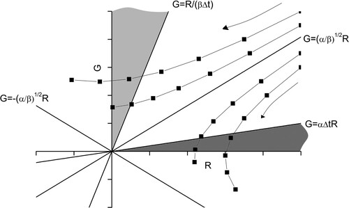In this case, the eigenvectors of K form an inset $G=\sqrt{(\alpha /\beta )}R$ and outset $G=-\sqrt{(\alpha /\beta )}R$ with the origin as a saddle. This is illustrated in Figure 1 which shows that for $(1/\beta \mathrm{\Delta }t)\ge \alpha \mathrm{\Delta }t$ the overall dynamics is determined by whether the starting point is above or below the inset. Thus, for initial conditions G₀ and R₀, if (11) $\begin{array}{rl}\beta G_0^2-\alpha R_0^2& >0\text{ Green wins}\\ \beta G_0^2-\alpha R_0^2& <0\text{ Red wins}\\ \beta G_0^2-\alpha R_0^2& =0\text{ mutual destruction}\text{.}\end{array}$(11)

Figure 1. A typical phase space diagram corresponding to (5) for $(1/\beta \mathrm{\Delta }t)>\alpha \mathrm{\Delta }t$ with inset $G=\sqrt{(\alpha /\beta )}R$ and outset $G=-\sqrt{(\alpha /\beta )}R$. Once a trajectory enters the light grey region Green will win by the end of the current battle, and once a trajectory enters the grey region Red will win by the end of the current battle. Representative trajectories (squares joined with lines) are shown on either side of the inset $G=\sqrt{(\alpha /\beta )}R$. The arrows indicate the movement of the trajectories under iteration.

Using (10) we can estimate the number of battles until defeat by solving for $G_n=0$ or $R_n=0$ . This gives (12) $n\simeq \frac{2\ln \left(\sqrt{\alpha }{R}_0+\sqrt{\beta }{G}_0\right)-\ln (|\alpha R_0^2-\beta G_0^2|)}{\ln \left(1+\mathrm{\Delta }t\sqrt{\alpha \beta }\right)-\ln \left(1-\mathrm{\Delta }t\sqrt{\alpha \beta }\right)}$(12)

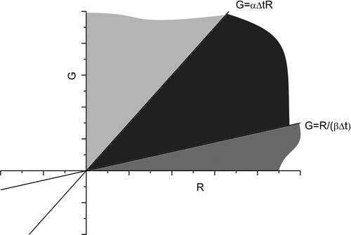
The dynamics of the model become simpler if $(1/\beta \mathrm{\Delta }t)<\alpha \mathrm{\Delta }t$ with (5) meaning the victor, or mutual destruction, are determined after only one battle (see Figure 2) where, if (13) $\begin{array}{rl}{G}_0& >\alpha \mathrm{\Delta }t{R}_0\text{ Green wins}\\ G_0& <\frac{1}{\beta \mathrm{\Delta }t}{R}_0\text{ Red wins}\\ \alpha \mathrm{\Delta }t{R}_0& \ge G_0\ge \frac{1}{\beta \mathrm{\Delta }t}{R}_0\text{ mutual destruction}\text{.}\end{array}$(13)

Figure 2. A typical phase space diagram corresponding to (5) for $(1/\beta \mathrm{\Delta }t)<\alpha \mathrm{\Delta }t$. In this case defeat is obtained after one battle. If the initial force levels lie in the light grey region Green wins. If they lie in the grey region Red wins. If they lie in the dark grey region we have a mutual destruction with both forces being annihilated by the end of the battle

3. Lanchester’s Model with constant reinforcements

Given that we are considering each iteration of (5) to represent an individual battle it is natural to allow for the possibility that after each battle, assuming an outright victory has not been achieved by one side, reinforcements can be added to each side before the commencement of the next battle.

Let us assume that Red and Green have a constant supply of new forces which can be added in amounts R^R and G^R at the beginning of each new battle. This gives rise to the new model (14) $\begin{array}{rl}{G}_{i+1}& =\{\begin{array}{cc}{G}_i-\alpha \mathrm{\Delta }t{R}_i+G^R& if{G}_i-\alpha \mathrm{\Delta }t{R}_i>0\\ 0& if{G}_i-\alpha \mathrm{\Delta }t{R}_i\le 0\end{array}\\ R_{i+1}& =\{\begin{array}{cc}{R}_i-\beta \mathrm{\Delta }t{G}_i+R^R& if{R}_i-\beta \mathrm{\Delta }t{G}_i>0\\ 0& if{R}_i-\beta \mathrm{\Delta }t{G}_i\le 0\end{array}\end{array}$(14) The if conditions in (14) account for the fact that if by the end of the i^th battle one side has been defeated then the war is assumed to be over and no reinforcements are added.

Assuming $G_i-\alpha \mathrm{\Delta }t{R}_i>0$ and $R_i-\beta \mathrm{\Delta }t{G}_i>0$ we can write (14) as (15) ${\underset{\_}{A}}_{i+1}=K{\underset{\_}{A}}_i+\underset{\_}{\mathrm{\Re }}$(15) where $\underset{\_}{\mathrm{\Re }}=\left[\begin{array}{c}{G}^R\\ R^R\end{array}\right]$. This inhomogeneous system can be transformed to a homogeneous system (16) ${\underset{\_}{X}}_{i+1}=K{\underset{\_}{X}}_i$(16) where the system has been centred around the fixed point ${\underset{\_}{A}}^{\ast }$ of (15) via (17) ${\underset{\_}{X}}_i={\underset{\_}{A}}_i-{\underset{\_}{A}}^{\ast }$(17) and (18) ${\underset{\_}{A}}^{\ast }=\left[\begin{array}{c}{\displaystyle \frac{R^R}{\beta \mathrm{\Delta }t}}\\ {\displaystyle \frac{G^R}{\alpha \mathrm{\Delta }t}}\end{array}\right]$(18)

As with our original model, this system is most easily investigated by considering the behaviour of solution trajectories in the phase plane. The eigenvalues and eigenvectors giving rise to the inset and outset remain the same (as the matrix K is unchanged). However, instead of being centred on the origin the inset and outset are now centred on the fixed point with equations for the inset and outset being respectively, (19) $\begin{array}{rl}G& =\sqrt{\frac{\alpha }{\beta }}R+\frac{R^R}{\beta \mathrm{\Delta }t}-\sqrt{\frac{\alpha }{\beta }}\frac{G^R}{\alpha \mathrm{\Delta }t}\\ G& =-\sqrt{\frac{\alpha }{\beta }}R+\frac{R^R}{\beta \mathrm{\Delta }t}+\sqrt{\frac{\alpha }{\beta }}\frac{G^R}{\alpha \mathrm{\Delta }t}.\end{array}$(19)

In Figure 3 the inset and outset are labelled as lines S1 and S2 respectively. Note that the overall form of the trajectories in Figure 3 is the same as Figure 2, with two significant changes: First, all four regions created by the inset and outset are now ‘battle relevant’. Secondly, the single criterion of being in a particular quadrant as defined by the inset and outset does not necessarily determine the outcome. This is highlighted in Figure 4 where the region bounded by the R axis, S1 and $G=\alpha \mathrm{\Delta }tR$ results in a win for Green, because the conflict will be over by the end of the first battle.

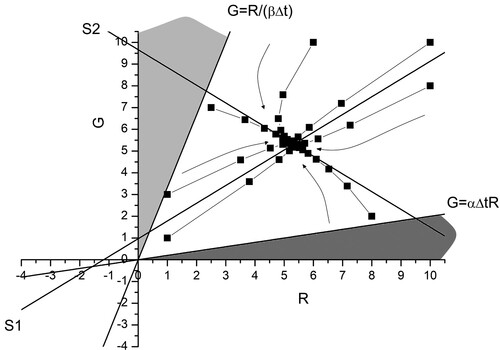
Figure 3. A typical phase space diagram corresponding to the constant reinforcement model (15) for $(1/\beta \mathrm{\Delta }t)>\alpha \mathrm{\Delta }t$ with the form of the inset S1 and outset S2 being given by (19). Once a trajectory enters the light grey region Green will win by the end of the current battle, and once a trajectory enters the grey region Red will win by the end of the current battle. Representative trajectories (squares joined with lines) are shown. The arrows indicate the movement of the trajectories under iteration.

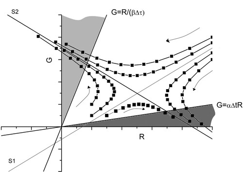
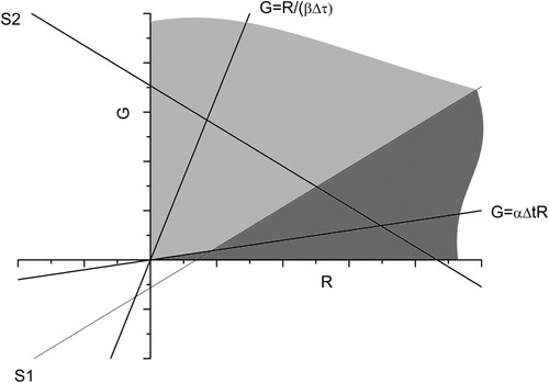
Figure 4. Same as Figure 3, but this time highlighting the regions of (R,G) space where victory for each side occurs. In the light grey region Green wins, in the grey region Red wins.

One final point on Figure 3 is that it provides commanders with a potential strategy diagram. Thus, for example, if the commander of the Green forces determines that he is on the right quadrant and is destined for defeat then if he can add, as a one off, a significant enough level of reinforcements before the next battle to move his army into the top quadrant then Green will ultimately win. This of course assumes that Red does not change her strategy. Further, the earlier he does this the less forces he will have to add to change the overall outcome. This means that if a relatively small number of extra reserve troops are added early on they may tip the battle. This is more likely to succeed if the opponent does not notice this change until the one off troop change she would have to introduce to move quadrant is beyond her reserve capabilities.

4. Lanchester’s Model with variable reinforcements

A more realistic form of reinforcement is to make the reinforcement level a function of the number of soldiers remaining after the previous battle (ie a function of $G_i-\alpha \mathrm{\Delta }t{R}_i$ for Green and of $R_i-\beta \mathrm{\Delta }t{G}_i$ for Red). We expect this functional form to be such that the reinforcements will be large when the number of soldiers remaining after the last battle is small, and to decrease with increasing soldier levels. Simple linear functional forms for Green and Red reinforcements respectively are (20) $\begin{array}{rl}{F}_G(G_i,R_i)& =G^R\left(1-\frac{1}{\gamma }(G{}_i-\alpha \mathrm{\Delta }t{R}_i)\right)\\ F_R(G_i,R_i)& =R^R\left(1-\frac{1}{\delta }(R{}_i-\beta \mathrm{\Delta }t{G}_i)\right).\end{array}$(20) where $G^R\text{ and }{R}^R$ are the maximum reinforcement levels for Green and Red and γ and δ are soldier levels (assumed to be greater than $G^R\text{ and }{R}^R$) above which instead of reinforcements being added to the battlefield they are instead removed (as F_G and F_R become negative). This troop removal scenario will not occur provided initial troop levels for Green and Red are assumed to be less than γ and δ respectively.

Our new model now becomes (21) $\begin{array}{rl}{G}_{i+1}& =\{\begin{array}{cc}{G}_i-\alpha \mathrm{\Delta }t{R}_i+F_G(G_i,R_i)& if{G}_i-\alpha \mathrm{\Delta }t{R}_i>0\\ 0& if{G}_i-\alpha \mathrm{\Delta }t{R}_i\le 0\end{array}\\ R_{i+1}& =\{\begin{array}{cc}{R}_i-\beta \mathrm{\Delta }t{G}_i+F_R(G_i,R_i)& if{R}_i-\beta \mathrm{\Delta }t{G}_i>0\\ 0& if{R}_i-\beta \mathrm{\Delta }t{G}_i\le 0.\end{array}\end{array}$(21) Assuming $G_i-\alpha \mathrm{\Delta }t{R}_i>0$ and $R_i-\beta \mathrm{\Delta }t{G}_i>0$ we can write (21) in matrix form as (22) ${\underset{\_}{A}}_{i+1}=L{\underset{\_}{A}}_i+\underset{\_}{\mathrm{\Re }}$(22) where ${\underset{\_}{A}}_i$ and $\underset{\_}{\mathrm{\Re }}$ are as defined previously and (23) $L=\left(\begin{array}{cc}\left(1-{\displaystyle \frac{G^R}{\gamma }}\right)& -\left(1-{\displaystyle \frac{G^R}{\gamma }}\right)\alpha \mathrm{\Delta }t\\ -\left(1-{\displaystyle \frac{R^R}{\delta }}\right)\beta \mathrm{\Delta }t& \left(1-{\displaystyle \frac{R^R}{\delta }}\right)\end{array}\right)$(23)

Thus, while our model has been extended to allow for dynamic changes in reinforcement levels after each battle, the fact that we have chosen the reinforcements to follow a linear law (20) means that mathematically speaking our model is unchanged. We still have a linear system of the form (22) which can be investigated via the use of eigenvalues, eigenvectors and fixed points, though as we shall see below, significantly our system now allows for a stable fixed point.

To simplify our analysis let us assume that Red and Green have similar reinforcement strategies and (24) $\frac{G^R}{\gamma }=\frac{R^R}{\delta }=\frac{1}{2}$(24)

Thus, for both Red and Green if troop levels at the end of a battle are equal to twice the maximum reinforcement levels no new soldiers will be added. This immediately gives (25) $L=\frac{1}{2}K$(25)

The eigenvalues and eigenvectors of L are (26) $\lambda =\frac{1}{2}\left(1\pm \mathrm{\Delta }t\sqrt{\alpha \beta }\right)$(26) and (27) $\underset{\_}{e}=\left[\begin{array}{c}1\\ \mp \sqrt{\frac{\beta }{\alpha }}\end{array}\right]$(27) and the fixed point of (22) is (28) ${\underset{\_}{A}}^{\ast }=\left[\begin{array}{c}\frac{2(G^R-\alpha \mathrm{\Delta }t{R}^R)}{1-\alpha \beta {(\mathrm{\Delta }t)}^2}\\ \frac{2(R^R-\beta \mathrm{\Delta }t{G}^R)}{1-\alpha \beta {(\mathrm{\Delta }t)}^2}\end{array}\right]$(28)

From (26), provided $\mathrm{\Delta }t\sqrt{\alpha \beta }<1$ both eigenvalues of L will lie between 0 and 1 and we will have a stable fixed point. Figure 5 gives an example of the evolution of the trajectories in this case. The key point here is that under the circumstances illustrated in Figure 5, the warfare reaches a stalemate with each side repeatedly adding reinforcements but failing to reach victory. This stalemate can be avoided if the fixed point (28) lies within either the light grey or grey regions, which will result in a victory for Green or Red respectively.

Figure 5. A typical phase space diagram for corresponding to the linear reinforcement model (22) for $(1/\beta \mathrm{\Delta }t)>\alpha \mathrm{\Delta }t$ and $(G^R/\gamma )=(R^R/\delta )=(1/2)$. Representative trajectories (squares joined with lines) are shown. All trajectories evolve towards the fixed point (28). Insets are labelled S1 and S2. The evaluation of the equations of S1 and S2 is left as an exercise for the reader (question 4 of Classroom Exercises).

5. Conclusions

Re-formulating Lanchester’s ‘aimed fire’ model (1) in discrete time furnishes the student not only with a new model based on repeated battle iterations, but also allows the inclusion of adding reinforcements between battles to be done in a straightforward manner. It allows for an illustration of the links between solution of coupled equations in discrete and continuous time, highlighting as it does analogues in analysis via eigenvalues, eigenvectors and phase plane analysis. Though such analysis is common in continuous time dynamical systems it is perhaps less familiar, but no less useful, in discrete time.

6. Classroom Exercises

1. By taking the equations for Lanchester’s aimed fire model (1), dividing one by the other and solving show that (1) results in the so-called ‘law of squares’, (29) $\beta G^2-\alpha R^2\text{ = constant}$(29)

Given this, what are the criteria for who ultimately wins? How does this compare to the criteria for the discrete time model? What is the corresponding solution for the unaimed fire model (2)?

1. Figures 3 and 4 consider the constant reinforcement model (14) when $(1/\beta \mathrm{\Delta }t)>\alpha \mathrm{\Delta }t$. What happens when $(1/\beta \mathrm{\Delta }t)<\alpha \mathrm{\Delta }t$?

2. In considering the variable reinforcement levels the ratio$(G^R/\gamma )=(R^R/\delta )=(1/2)$ was chosen. Show that more generally if $(G^R/\gamma )=(R^R/\delta )=f$ the fixed point of (22) is (30) ${\underset{\_}{A}}^{\ast }=\left[\begin{array}{c}{\displaystyle \frac{\alpha \mathrm{\Delta }tf{R}^R-(1-f)G^R}{\alpha \beta {(\mathrm{\Delta }t)}^2{f}^2-{(1-f)}^2}}\\ {\displaystyle \frac{\beta \mathrm{\Delta }tf{G}^R-(1-f)R^R}{\alpha \beta {(\mathrm{\Delta }t)}^2{f}^2-{(1-f)}^2}}\end{array}\right]$(30)

What are the eigenvalues and eigenvectors of the system? Hint: Note that in calculating the eigenvalues, we are solving $|fK-\lambda I|=0$ where we already know that the eigenvalues of K to be given by (8) and in finding the eigenvectors we are solving $(fK-\lambda I)\underset{\_}{e}=\underset{\_}{0}$.

1. What are the equations of the insets S1 an S2 shown in Figure 5?

2. In the main body of the paper it is stated that in (20) γ and δ are assumed to be greater than $G^R\text{ and }{R}^R$ respectively. What happens if this is not the case?

3. In the main body of the paper it is noted that a stalemate for the linear reinforcement model can be avoided if the fixed point (28) can be moved into the grey or light grey regions of Figure 5. For these cases, derive inequalities which give conditions for Green or Red victory

4. While this paper emphasizes the usefulness of illustrating the solution of Lanchester’s Equations in discrete time, via the phase plane it can also be helpful to illustrate their behaviour via time series. By assuming the ratios given in (24), make representative choices of the remaining parameters and write a short computer code to generate time-series for G_i and R_i which correspond to the behaviours illustrated in Figures 3 and 5.

Disclosure statement

No potential conflict of interest was reported by the author.

References

- Bracken, J. (1995). Lanchester models of the Ardennes campaign. Naval Research Logistics, 42(5), 559–577. https://doi.org/10.1002/1520-6750(199506)42:4<559::AID-NAV3220420405>3.0.CO;2-R
- Clifton, E. (2020). ‘A brief review on the application of Lanchester’s models of combat in nonhuman animals. Ecological Psychology, 32(4), 181–191. https://doi.org/10.1080/10407413.2020.1846456
- Elaydi, S. N. (2008). Discrete chaos (2/e). Chapman & Hall/CRC.
- Johnson, D. D. P., & MacKay, N. J. (2015). Fight the power: Lanchester’s laws of combat in human evolution. Evolution and Human Behavior, 36(2), 152–163. https://doi.org/10.1016/j.evolhum-behav.2014.11.001
- Lanchester, F. W. (1916). Aircraft in warfare: The Dawn of the fourth Arm. Constable & Co.
- MacKay, N. (2006). Lanchester combat models. Mathematics Today, 42(5), 170–173.
- MacKay, N. (2015). When Lanchester met richardson, the outcome was stalemate: A parable for mathematical models of insurgency. Journal of the Operational Research Society, 66(2), 191–201. https://doi.org/10.1057/jors.2013.178
- MacKay, N. (2020). When Lanchester met Richardson: The interaction of warfare with psychology. In N. P. Gleditsch (Ed.), Lewis Fry Richardson: His intellectual legacy and influence in the social sciences (pp. 101–112). Springer Open.
- MacKay, N., & Johnson, I. (2011). Lanchester models and the battle of Britain. Naval Research Logistics, 58(3), 210–222. https://doi.org/10.1002/nav.20328
- MacKay, N., Price, C., & Wood, A. J. (2016). Weight of shell must tell: A Lanchestrian reappraisal of the battle of Jutland. Journal of the Historical Association, 101(347), 536–563. https://doi.org/10.1111/1468-229X.12241
- McCartney, M. (1997). Triple and double step wave functions for two electron atoms. European Journal of Physics, 18(2), 90–93. https://doi.org/10.1088/0143-0807/18/2/006
- McCartney, M., & Bradley, E. (2019). Four hundred years of the fractal coastline of Scotland. The Mathematical Gazette, 103(558), 518–521. https://doi.org/10.1017/mag.2019.120
- McCartney, M., & Carey, M. (2000). Follow that car! investigating a simple class of car following model. Teaching Mathematics and its Applications, 19(2), 83–87. https://doi.org/10.1093/teamat/19.2.83
- Willard, D. (1962). Lanchester as a force in history: an analysis of land battles of the years 1618-1905. Research Analysis Corporation, Bethesda MD, Report No. RAC-TP-74.