Four variations on a fractal theme

Abstract

Four variations of the Koch curve are presented. In each case, the similarity dimension, area bounded by the fractal and its initiator, and volume of revolution about the initiator are calculated. A range of classroom exercises are proved to allow students to investigate the fractals further.

KEYWORDS:

• Fractals
• Pappus
• Koch curve

1. Introduction

The Koch curve is a standard introductory example of a fractal given in textbooks (see for example Addison, 1997; Frame & Urry, 2016; Goodson, 2017; Kautz, 2011; Peitgen et al., 1992; Strogatz, 2014; Tél & Gruiz, 2006). Typically, as von Koch did when he introduced the curve (von Koch, 1904), introductions emphasize that the curve possesses no tangents and also note that it has divergent length, and evaluate its similarity dimension. But they then tend to move on to other examples of fractals (e.g. the Cantor dust, or Sierpinski triangle or carpet). Exceptions to this are Tél and Gruiz (2006, pp. 30–31), Mandelbrot (1983, pp. 56–57) and Frame and Urry (2016, p. 167) who each give illustrations of some variants of the Koch curve but do not investigate them in any detail.

In this note, we consider four variations on the Koch curve which can be investigated by students in the classroom and in each case we evaluate their similarity dimension, the area bounded by the curve and the initiator and the volume of revolution.

2. Cesàro curves

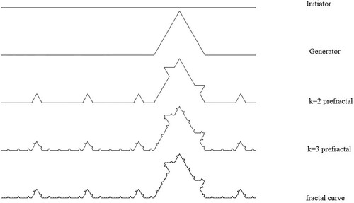
The Koch curve is based on a generating curve where the central third of an initiating line of unit length is replaced with the upper two lines of an equilateral triangle. An obvious generalization of this is to instead use the equal sides of an isosceles triangle such that all four lines of the generator are of equal length (Figure 1). 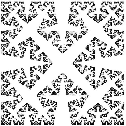It is straightforward to show that, in the initiator is of unit length, the generating curve is made up of segments of length, (1) $\begin{array}{r}L=\frac{1}{2(1+\cos \theta )}.\end{array}$(1) If four such Cesàro curves are placed in a square formation with the curves pointing inwards the result is called a torn square fractal (Figure 2).

Figure 1. Constructing a Cesàro curve with $\theta ={45}^{\circ }$. The initiator (k = 0 iteration) is a straight line of unit length. The generator is constructed by replacing the centre of the initiator with the upper part of an isosceles triangle such that each line of the generator is of length $L=\frac{1}{2(1+\cos \theta )}$ and thus the distance from end to end of the generator is also unity. The k = 2 pre-fractal is constructed by replacing each straight line of the with a scaled version of the generator. Replacing each straight line in the k = 2 pre-fractal with a scaled version of the generator results in k = 3. Repeating this process an infinite number of times produces the fractal.

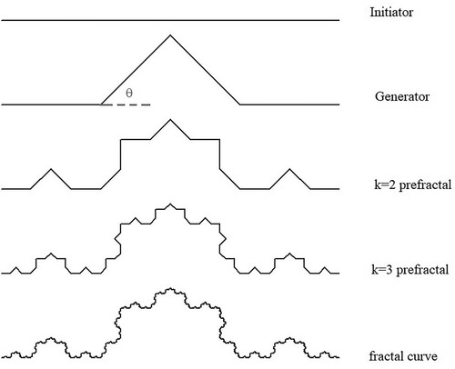
Figure 2. An example of a torn square fractal made up of four a Cesàro curves with $\theta ={80}^{\circ }$.

Cesàro curves are frequently defined in terms of segment lengths, L of their generator (see for example Frame & Urry, 2016, p. 167; Tél & Gruiz, 2006, pp. 30–31), but we shall instead use the angle $\theta$.

The similarity dimension of a fractal is defined as (2) $\begin{array}{r}{D}_s=\frac{\log (N)}{\log (1/\epsilon )}\end{array}$(2) where if we scaled the fractal by a factor $\epsilon$ we would require N copies of it to reconstruct the original fractal. Thus if we scale a Cesàro curve by a factor of L we will need N = 4 copies of it to reconstruct the original fractal and so, (3) $\begin{array}{r}{D}_S=\frac{\log (4)}{\log (2(1+\cos \theta ))}.\end{array}$(3)

To evaluate the area and volume of revolution about the initiator of a Cesàro curve we use the method outlined in McCartney (2021).

Figure 3 shows a Cesàro curve divided into its component self-similar areas. If we define the area bounded by the curve and its initiator is $A_{\mathrm{\infty }}$ then clearly (4) $\begin{array}{r}{A}_{\mathrm{\infty }}=4A_S+A_T.\end{array}$(4)

Figure 3. A Cesàro curve divided into its component self-similar areas.

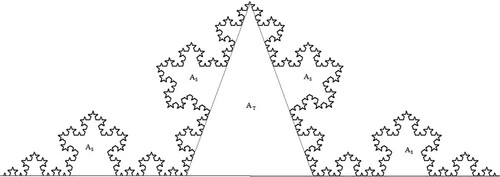
But, by definition, each of the four areas $A_S$ is a scaled version of the entire bounded area. The length is scaled by a factor L and therefore the area is scaled by L², giving (5) $\begin{array}{r}{A}_s=L^2{A}_{\mathrm{\infty }}.\end{array}$(5)

Since the area of the isosceles triangle is (6) $\begin{array}{r}{A}_T=L^2\cos \theta \sin \theta \end{array}$(6) (4) becomes (7) $\begin{array}{r}{A}_{\mathrm{\infty }}=4L^2{A}_{\mathrm{\infty }}+L^2\cos \theta \sin \theta \end{array}$(7) which, using (1) simplifies to (8) $\begin{array}{r}{A}_{\mathrm{\infty }}=\frac{\sin \theta }{4(\cos \theta +2)}.\end{array}$(8)

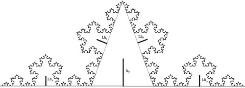
To evaluate the volume of revolution we first evaluate the centre of area of the curve bounded by its initiator. If the centre of area is a distance h_y above the initiating line along the axis of symmetry, then (from Figure 4) we can consider again the fact that the total area is made up of the triangle of area A_T (with centre of area $(L\sin \theta )/3$ above its base) and the four areas A_S, each having centres od area a distance Lh_y above their corresponding initiating lines. We can thus write the moment of area as (9) $\begin{array}{r}{A}_{\mathrm{\infty }}{h}_y=A_T\frac{L}{3}\sin \theta +2h_{y}L{A}_s+2A_s\left(h_{y}L\cos \theta +\frac{L}{2}\sin \theta \right).\end{array}$(9) Using (1), (5), (6) and (8) this simplifies to give (10) $\begin{array}{r}{h}_y=\frac{1}{6}\tan \left(\frac{\theta }{2}\right).\end{array}$(10)

Figure 4. The centre of area of a Cesàro curve lies a distance h_y above the initiating line along the axis of symmetry.

Given the second theorem of Pappus, which states that the volume of revolution of a lamina about an axis is the area of the lamina multiplied by the distance travelled by the lamina’s centroid we can immediately write that the volume of revolution of the Cesàro curve about the initiating axis is (11) $\begin{array}{r}{V}_C=\frac{\pi }{12}\frac{1-\cos \theta }{2+\cos \theta }.\end{array}$(11)

3. An n-Koch curve

In the Koch curve, we divide the initiator into three equal segments and replace the middle third with the upper two lines of an equilateral triangle. A variation on this is to divide the initiator into n equal segments and to replace one of these with the upper lines of an equilateral triangle (Figure 5).

Figure 5. The construction of an n-Koch curve with n = 5, and the penultimate segment of the initiator being chosen for replacement.

Given we need n + 1 copies of the original fractal scaled by a factor of 1/n to reproduce the fractal the similarity dimension is, (12) $\begin{array}{r}{D}_S=\frac{\log (n+1)}{\log (n)}.\end{array}$(12)

To evaluate the area enclosed by the fractal and its initiating line, $A_{\mathrm{\infty }}$, we follow the same procedure as before. Namely that this area must be equal to the area of the generating triangle, (13) $\begin{array}{r}{A}_T=\frac{\sqrt{3}}{4n^2}\end{array}$(13) plus the area of n + 1 scaled copies of the fractal each of which are of area, (14) $\begin{array}{r}{A}_S=\frac{1}{n^2}{A}_{\mathrm{\infty }}\end{array}$(14) giving (15) $\begin{array}{r}{A}_{\mathrm{\infty }}=A_T+(n+1)A_S\end{array}$(15) which leads directly to (16) $\begin{array}{r}{A}_{\mathrm{\infty }}=\frac{\sqrt{3}}{4(n^2-n-1)}.\end{array}$(16)

To evaluate the volume of revolution we first evaluate the centre of area of the curve bounded by its initiator. If the centre of area is at $(h_x,h_y)$ then (from Figure 6) we can consider again the fact that the total area is made up of the triangle of area A_T (with centre of area $\frac{1}{2\sqrt{3}n}$ above its base) and the n + 1 areas A_S, each having centres of area scaled by a factor of 1/n. We can thus write the moment of area as (17) $\begin{array}{r}{A}_{\mathrm{\infty }}{h}_y=(n-1)A_S\frac{h_y}{n}+A_S\left(\frac{h_x}{n}\frac{\sqrt{3}}{2}+\frac{h_y}{n}\frac{1}{2}\right)+A_S\left(\frac{1-h_x}{n}\frac{\sqrt{3}}{2}+\frac{h_y}{n}\frac{1}{2}\right)+A_T\frac{1}{2\sqrt{3}n}\end{array}$(17) which results in (18) $\begin{array}{r}{h}_y=\frac{1}{2\sqrt{3}}\frac{n^2-n+2}{n(n^2-1)}\end{array}$(18) and hence a volume of revolution about the initiator is (19) $\begin{array}{r}{V}_{nK}=\frac{\pi (n^2-n+2)}{4n(n^2-1)(n^2-n-1)}.\end{array}$(19)

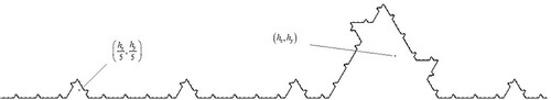
Figure 6. The centre of area of an n-Koch curve with n = 5. Considering the leftmost point of the fractal to be the origin and the initiating line to be the x axis, the centre of area of the lamina bounded by the curve and the initiator is defined as $(h_x,h_y)$. The centre of area of each segment is scaled by a factor of n, so in the case where n = 5 the co-ordinates of the centre of area of the first segment is $\left(\frac{h_x}{5},\frac{h_y}{5}\right)$.

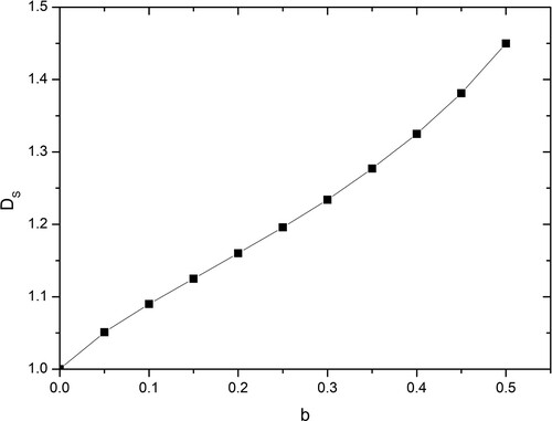
4. A Koch curve with non-uniform scaling

So far we have considered fractal curves made up of line segments of equal length, but it is straightforward to generalize this. As an example, consider an initiator of unit length where we replace a middle length b with the upper two lines of an equilateral triangle to produce a generator (Figure 7). Each line is then replaced with a suitable scaled version (b or $1-b/2$) of the generator to produce the k = 2 pre-fractal. Figure 8 shows a range of fractals generated using b = 0.1, b = 0.25, b = 0.5.

Figure 7. The construction of a Koch curve with nonuniform scaling. The initiator is of length unity. The central upper sides of the equilateral triangle in the generator are of length b, with the other two lines being of length $\left(\frac{1-b}{2}\right)$.

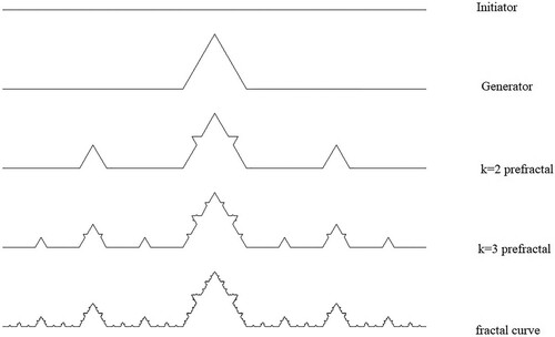
Figure 8. A range of nonuniform scalings. From top to bottom, b = 0.1, b = 0.25, b = 0.5. For values of b greater than approximately 0.5 the curve begins to self-intersect.

To evaluate the similarity of the fractal we use Moran’s equation (see Frame & Urry, 2016, p. 163) which states that if we have a fractal which is created by N copies of itself, each scaled by a different factor ${\epsilon }_1,{\epsilon }_2,\dots {\epsilon }_N$ then the similarity dimension $D_S$ is given by the solution of (20) $\begin{array}{r}\sum _{i=1}^N{\epsilon }_i^{D_s}=1.\end{array}$(20) Thus, for the fractal described here Moran’s equation becomes, (21) $\begin{array}{r}2b^{D_S}+2{\left(\frac{1-b}{2}\right)}^{D_S}=1.\end{array}$(21)

A plot of a numerical solution of this is shown in Figure 9 (see Classroom exercises for an exact solution when $b=1/2$).

Figure 9. Variation of similarity dimension $D_S$ with scaling factor b as given by (21) for the non-uniform scaling Koch curve shown in Figure 7.

To evaluate $A_{\mathrm{\infty }}$, the area bounded by the non-uniform scaling Koch curve and its initiator, we apply the same procedure as before. Namely, the area must be made up of two copies scaled at b, two at $1-b/2$, and the triangle in the generator, which is of area, (22) $\begin{array}{r}{A}_T=\frac{\sqrt{3}}{4}{b}^2\end{array}$(22)

Thus, (23) $\begin{array}{r}{A}_{\mathrm{\infty }}=2b^2{A}_{\mathrm{\infty }}+2{\left(\frac{1-b}{2}\right)}^2{A}_{\mathrm{\infty }}+A_T\end{array}$(23) which results in, (24) $\begin{array}{r}{A}_{\mathrm{\infty }}=\frac{\sqrt{3}{b}^2}{2(1+2b-5b^2)}.\end{array}$(24)

Finally, to evaluate the volume of revolution we first evaluate the centre of area above the initiating line, h, as being constructed from the centres of area of the two pairs of scaled copies of the fractal plus the centre of area of the triangle in the generator, giving (25) $\begin{array}{r}{A}_{\mathrm{\infty }}h=2h{\left(\frac{1-b}{2}\right)}^3{A}_{\mathrm{\infty }}+2b^2{A}_{\mathrm{\infty }}\left(\frac{hb}{2}+\frac{\sqrt{3}b}{4}\right)+A_T\frac{b}{3}\frac{\sqrt{3}}{2}\end{array}$(25) which, using (22) and (24), results in (26) $\begin{array}{r}h=\frac{\sqrt{3}b}{9(1-b)}\end{array}$(26) giving a volume of revolution about the initiator of (27) $\begin{array}{r}{V}_S=\frac{\pi b^3}{3(1-b)(1+2b-5b^2)}.\end{array}$(27)

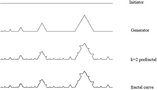
5. A Himalayan Koch curve

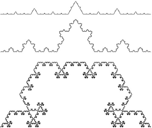
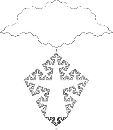
Finally, we consider a fractal where the generator is made up of an infinite array of Koch curve generators scaled geometrically; each a factor $\alpha$ smaller than the last (Figures 10 and 11).

Figure 10. The Construction of a Himalayan Koch curve with scale factor $\alpha =\frac{1}{2}$. The generating line is made up of an infinite array of generators for the standard Koch curve, each a scaled version (by a factor of $\alpha$) of the generator to its right. Each line of each of these scaled Koch generators is then replaced by a suitably scaled version of the total generating line to form the k = 2 pre-fractal.

Given the length of the initiator is unity and assuming the rightmost generating Koch curve in Figure 10 is of length L, clearly $1=L\sum _{i=0}^{\mathrm{\infty }}{\alpha }^i$ and so (28) $\begin{array}{r}L=1-\alpha .\end{array}$(28)

To evaluate the similarity dimension, we once again turn to Moran’s equation. Each of the generating Koch curves is made up of four lines of length $\frac{L}{3}{\alpha }^i$ and so using (20) (29) $\begin{array}{r}4\sum _{i=0}^{\mathrm{\infty }}{\left[\frac{L{\alpha }^i}{3}\right]}^{D_S}=1\end{array}$(29) and summing the series gives (30) $\begin{array}{r}\frac{4}{3^{D_S}}\frac{{(1-\alpha )}^{D_S}}{1-{\alpha }^{D_S}}=1.\end{array}$(30)

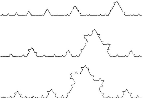
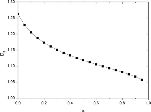
A plot of a numerical solution of this equation is shown in Figure 12.

Figure 11. Himalayan k = 3 pre-fractals with scale factors (from top to bottom) $\alpha =\frac{2}{3},\frac{1}{3},\frac{1}{5}$.

The area bounded by the generator and the initiator is the geometric sum of the areas of the triangles, giving (31) $\begin{array}{r}{A}_T=\frac{\sqrt{3}}{36}\frac{1-\alpha }{1+\alpha }.\end{array}$(31) The area of the fractal bounded by its initiator is made up of sets of four copies each scaled by in length by $\frac{L}{3}{\alpha }^i$, and hence by area ${\left(\frac{L}{3}\right)}^2{\alpha }^{2i}$, plus the area A_T i.e. (32) $\begin{array}{r}{A}_{\mathrm{\infty }}=4A_{\mathrm{\infty }}\sum _{i=0}^{\mathrm{\infty }}{\left(\frac{L}{3}\right)}^2{\alpha }^{2i}+A_T\end{array}$(32) which using (28) and (31) results in, (33) $\begin{array}{r}{A}_{\mathrm{\infty }}=\frac{\sqrt{3}}{4}\frac{1-\alpha }{5+13\alpha }\end{array}$(33)

To evaluate the centre of area of the fractal, located at $(h_x,h_y)$ we first evaluate the moment of area of each section of the fractal constructed on each of the Koch curve generators. Counting from the right of the fractal shown in Figure 10, the total length of the ith Koch curve generator be (34) $\begin{array}{r}{L}_i=(1-\alpha ){\alpha }^{i-1}\end{array}$(34)

Thus the moment of area of the ith section $M_i$ is constructed from four components each made up of versions of the original fractal scaled in size by $\frac{L_i}{3}$ plus the moment of area of the equilateral triangle of side $\frac{L_i}{3}$: (35) $\begin{array}{rl}{M}_i& =2h_y{\left(\frac{L_i}{3}\right)}^3{A}_{\mathrm{\infty }}+{\left(\frac{L_i}{3}\right)}^3\left(h_x\frac{\sqrt{3}}{2}+h_y\frac{1}{2}\right)A_{\mathrm{\infty }}\\ & +{\left(\frac{L_i}{3}\right)}^3\left((1-h_x)\frac{\sqrt{3}}{2}+h_y\frac{1}{2}\right)A_{\mathrm{\infty }}+\frac{1}{8}{\left(\frac{L_i}{3}\right)}^3\end{array}$(35)

Since the total moment of area obeys (36) $\begin{array}{r}{A}_{\mathrm{\infty }}{h}_y=\sum _{i=1}^{\mathrm{\infty }}{M}_i\end{array}$(36) and noting that (37) $\begin{array}{r}\sum _{i=1}^{\mathrm{\infty }}{L}_i^3=\frac{{(1-\alpha )}^3}{1-{\alpha }^3}\end{array}$(37) Equations (35) and (36) give (38) $\begin{array}{r}{h}_y=\frac{(1-\alpha )(5\alpha +4)}{3\sqrt{3}(8{\alpha }^2+11\alpha +4)}\end{array}$(38) which results in a volume of revolution about the initiator of (39) $\begin{array}{r}{V}_H=\frac{\pi {(1-\alpha )}^3(5\alpha +4)}{6(13\alpha +5)(8{\alpha }^2+11\alpha +8)}.\end{array}$(39)

6. Concluding remarks

The results presented here are all well within the reach of an undergraduate. Indeed, although the algebraic manipulation can in parts require care, the concepts behind the evaluation of the bounded area are also within reach of a good U.K. ‘A’ level student.

Further, given the Koch curve is almost certainly the most common fractal curve to be found in undergraduate curricula, hopefully these variations, combined with the classroom exercises below, will provide useful extensions to teaching, either as extra problems or as short independent study projects.

Figure 12. Variation of similarity dimension $D_S$ with scaling factor $\alpha$ as given by (30) for the non-uniform scaling Koch curve shown in Figure 10.

7. Classroom exercises

1. For a Koch curve with initiator of unit length, the area of the curve bounded by the initiator, and the distance of the centre of area above the initiator are $A_{\mathrm{\infty }}=\frac{\sqrt{3}}{20}$ and $h_y=\frac{\sqrt{3}}{18}$. Show that for appropriate parameter choices each of the areas and centres of areas presented in the paper reduce to these results.

2. Assuming the initiator is of length unity, what is the area bounded by a torn square fractal of the form shown in Figure 2 for a Cesàro curve of angle $\theta$?

3. Assuming that the initiator is of length unity, show that the distance of the centre of area of the right half of a Cesàro curve (ie the area bounded by the curve, its initiator, and the vertical axis of symmetry) is a distance $\frac{1}{6}\left(1-\frac{\cos \theta }{{(1+\cos \theta )}^2}\right)$ from the axis of symmetry. Hence evaluate the volume of revolution of the curve about its vertical axis of symmetry.

4. If three Koch curves are placed together around an equilateral triangle of unit side the Koch island, or Koch snowflake, is obtained (Figure 13). An obvious way to generalize this is to place three Cesàro curves around an isosceles triangle generating a Cesàro island (Figure 14). The two equal sides of the triangle are of unit length, and the equal angles are the same as those of the angle used to generate the Cesaro curves. Show that the area of such a Cesàro island is (40) $\begin{array}{r}{A}_I=\frac{\sin \theta {(2\cos \theta +1)}^2}{2(\cos \theta +2)}.\end{array}$(40) By plotting the above function (or otherwise) show that that maximum bounded area occurs at approximately $\frac{\pi }{4}$.

5. Show that the x co-ordinate $h_x$ of the centre of area of the n Koch curve (see Figure 6) is $\frac{n-1}{n+1}$ and hence find the volume of revolution about the vertical axis.

6. When $b=\frac{1}{2}$ Equation (21) can be written as, (41) $\begin{array}{r}2{\left(\frac{1}{2}\right)}^{D_S}+2{\left(\frac{1}{4}\right)}^{D_S}=1.\end{array}$(41)

1. Show that the solution of this equation is (42) $\begin{array}{r}{D}_S=1-\frac{\ln \left(\sqrt{3}-1\right)}{\ln 2}.\end{array}$(42)

2. Hint: re-write (41) as a quadratic equation.

3. A simple piece of python code, which uses a recursive function call to generate the kth pre-fractal of a Koch curve is:

4. import turtle as t

5. #this code generates a pre-fractal Koch curve with initiator length Size

6. #to level k

7. #set size and level of prefractal

8. k = 5

9. size = 600

10. #set position and speed of turtle and penwidth

11. t.hideturtle()

12. t.penup()

13. t.goto(-300,-50)

14. t.pendown()

15. t.pensize(1)

16. t.speed(0)

17. def koch(prefractal, size):

18.    if prefractal  = = 0:

19.       t.forward(size)

20.    else:

21.         for angle in [60, -120, 60, 0]:

22.            koch(prefractal-1, size/3)

23.            t.left(angle)

24. koch(k,size)

25. Modify this code to generate a Cesàro curve for a user provided $\theta$. Modify the code further to produce a torn square fractal.

26. In the construction of the Himalayan Koch curve in the paper a generator with an infinite geometric series of Koch curve generators was used as the generator. If a finite series of n Koch curve generators in geometric progression is used instead, what is the area bounded by the generator and the initiator? What is the area bounded by the fractal and the initiator?

Figure 13. The Koch island is obtained by taking three Koch curves and placing them around an equilateral triangle of unit side.

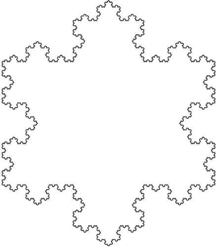
Figure 14. Two Cesàro islands. The equal length sides of the isosceles triangles on which the snowflakes are based are of length unity, the equal angle $\theta$ is the same as that use to generate the Cesàro curves. (a) $\theta ={30}^{\circ }$, (b) $\theta ={80}^{\circ }$.

Disclosure statement

No potential conflict of interest was reported by the author.

References

- Addison, P. S. (1997). Fractals and chaos: An illustrated course. IOP.
- Frame, M., & Urry, A. (2016). Fractal worlds: Grown, built and imagined. Yale University Press.
- Goodson, G. R. (2017). Chaotic dynamics: Fractals, tilings, and substitutions. Cambridge University Press.
- Kautz, R. (2011). Chaos: The science of unpredictable random motion. Oxford University Press.
- Mandelbrot, B. B. (1983). The fractal geometry of nature. W.H. Freeman & Co.
- McCartney, M. (2021). The area, centroid and volume of revolution of the Koch curve. International Journal of Mathematical Education in Science and Technology, 52(5), 782–786. https://doi.org/10.1080/0020739X.2020.1747649
- Peitgen, H., Jurgens, H., & Saupe, D. (1992). Chaos and fractals: New frontiers of science. Springer-Verlag.
- Strogatz, S. H. (2014). Nonlinear dynamics and chaos (2nd ed.). Westview Press.
- Tél, T., & Gruiz, M. (2006). Chaotic dynamics: An introduction based on classical mechanics. Cambridge University Press.
- von Koch, H. (1904). Sur une courbe continue sans tangente, obtenue par une construction géométrique élémentaire. Arkiv för Mathematik Astronomi och Fysik, 1, 681–704.