Modelling the flow through ion channels at the cell membrane

ABSTRACT

Mathematics provides us with tools to capture and explain phenomena in everyday biology, even at the nanoscale. The most regularly applied technique to biology is differential equations. In this article, we seek to present how differential equation models of biological phenomena, particularly the flow through ion channels, can be used to motivate and teach differential equations. Ion channels on the cell membrane allow the passage of ions from one side of the membrane to the other. The movement of these ions drives crucial processes such as the beating of our hearts. Using a system of two ordinary differential equations it is possible to capture the movement across ion channels that are opening and closing. Then using standard undergraduate techniques, we can predict how these channels behave in the long-term. In this work, we discuss how this example can be used to create tangible links to mathematical equations and motivate the teaching of techniques such as differentiation, integration, algebraic manipulation and equilibrium analysis. Furthermore, we show how a simple reformulation of this model into a stochastic setting using Gillespie's Stochastic Simulation Algorithm can allow us to capture the noise in ion channel flow.

KEYWORDS:

• Differential equations
• undergraduates
• integration
• modelling
• simulation
• education
• real-world mathematics

1. Introduction

Giving real-life, tangible meaning to mathematical formalisms has been known for some time to greatly assist in student learning (Gravemeijer & Doorman, 1999; Khotimah & Masduki, 2016; Kwon et al., 2016). By linking algebraic expressions to real-life situations, students can connect knowledge of something unknown (mathematics) with something well-known (real-life). In this way, students are provided with a bridge to improve their understanding of mathematics and make it an approachable subject for all demographics. The interaction between different specialisms is particularly important in mathematics, both to assist students in making sense of observed teaching and learning, and to help students become autonomous mathematicians (González-Martín et al., 2021).

In this article, we provide a description of a simple yet elegant real-world problem with its conjugate mathematical model. We detail how undergraduate level mathematical techniques can help us understand this problem and discuss how we can investigate randomness in this real-world situation very simply. This article provides a tool for educators to use when teaching differential equations. At the end, we detail ways in which this model could be extended for assignments or exams and what critical learning outcomes students would gain with this example.

1.1. What are ion channels and why are they important to model?

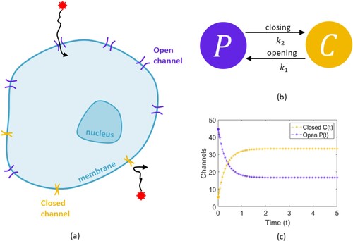
On the surface of cells, on the cell membrane, are ion channels. These channels are membrane proteins and are crucial for either allowing or blocking the flow of ions (such as Na⁺, K⁺, Ca²⁺, CI^-) in and out of a cell (Figure 1(a)). Ions are atoms that are either negatively or positively charged and their flow across ion channels of the cell control many crucial life processes. For example, the heart beat is controlled by the flow of ions in and out of the heart (Bartos et al., 2015). In a healthy heart, there is a balance between calcium (Ca²⁺) and potassium (K⁺) ion levels in both the outer and inner walls of the heart. That balance keeps electrical energy flowing correctly through the heart and allows the heart muscle to expand and contract as the heart beats. It is well accepted that individuals are extremely heterogeneous and will have different heart beat patterns. As such, the way in which their ion channels open and close will be very different. In addition, this process is highly random, i.e. stochastic, and so we need a way to capture the opening and closing of these channels so that we might better understand this process.

Figure 1. Schematic describing ion channel flow and the model formalism. (a) Charged ions travel across the membrane through open ion channels. These channels open and close to stop or encourage the flow of ions. This flow of ions controls the beating of our heart. (b) To capture the opening and closing of ion channels on a cell, consider the number of ion channels closed on a cell membrane to be represented by C and the number of open channels to be P. These channels then open and close at a rate given by $k_1$ and $k_2$ respectively. (c) Plot of the model showing the closed and open channels tending to a fixed number in time.

1.2. What are differential equations?

Mathematical discovery is largely driven by the desire to better understand reality (McCarthy et al., 2019). One area in which this is fundamental is in differential equation modelling. The simplest differential equations describe the rate of change of some quantity X over time: $\frac{dX}{dt}=f(t,X(t\left)\right))$ where f is a function describing the way in which the quantity X is changing in time t. The function f could be a function of time t and/or the quantity of interest $X\left(t\right)$. For example, if X was increasing at a constant rate a then $f(t,X(t\left)\right)=a$, where a>0. Whereas, if X was increasing at a rate proportional to itself then $f(t,X(t\left)\right))=\mathrm{aX}(t)$.

Mathematically, differential equations present an opportunity for undergraduates to test their understanding of a large number of learning outcomes in mathematics, including algebraic manipulation, differentiation, integration, stability analysis and simultaneous equations. In this work, we present the first educational example of an undergraduate level mathematical analysis and investigation of a model for ion channel flow. It is possible to extend this example to much more complicated differential equation models of ion channels (Pathmanathan & Gray, 2018; Tang & Wang, 2010), however we do not discuss those here. Examples of other teaching articles on real-world applications of differential equations can be found in the COVID-19 pandemic (Nelson, 2023), cancer (Beier et al., 2015), malaria (da Silva Soares & Borba, 2014) and many more.

2. An ion channel modelling problem

Simple and elegant differential equations are regularly used to capture biological phenomena and can assist in our understanding of mathematical foundations such as rates of change, gradients, differentiation and integration. A differential equation provides a measure for the change of a dependent variable given some independent variable. Furthermore, complementing mathematics education with biological examples has been shown to efficiently enhance student learning at all levels (Seshaiyer & Lenhart, 2020).

Consider a single cell and the ion channels on that cell, see Figure 1(a). These channels can either be open or closed, and whether they are open or closed will depend on time. This makes each channel's property either being ‘open’ or ‘closed’ a dependent variable, with time the independent variable. Linking mathematical expressions to represent variables is the first step of building a mathematical differential equation model for a biological system. In this example, we use a system of two ordinary differential equations (ODEs), one for the channels which are open and one for the channels which are closed.

Let $C\left(t\right)$ be the number of closed ion channels on a cell at time t, and $P\left(t\right)$ be the number of open ion channels at time t. We want to write down a differential equation that describes the change in C over time, and the change in P over time. Let us assume that closed channels open at a rate $k_1$ and open channels close at a rate $k_2$, see Figure 1(b). The rate of change of the number of closed ion channels is then: (1) $\frac{dC}{dt}=-k_{1}C+k_{2}P,$(1) and the rate of change of the number of open ion channels is: (2) $\frac{dP}{dt}=k_{1}C-k_{2}P.$(2) Ion channels on the cell open with rate $k_1$ and this rate is proportional to the number of channels that are closed and can be open, i.e. $C\left(t\right)$, hence the rate of change in the channels transitioning from closed to open is $k_{1}C$. This means that we will lose closed channels at a rate $k_{1}C$ and gain open channels at a rate $k_{1}C$. As such, this term will be negative in the rate of change of C and positive in the rate of change of P to reflect the gain and loss of these two populations. In a similar manner, the rate open channels close on the cell is given by $k_2$ and is proportional to the number of open channels that can close, i.e. $k_{2}P$ and hence there is a positive increase in the rate of change of the closed channels and a negative effect on the open channel population.

Both parameters, $k_1$ and $k_2$, in this model have units time${}^{-1}$. In this model, we assume there are no channels on the cell that aren't accounted for in C and P, and so the total channel number is $N=C\left(t\right)+P\left(t\right)$. Initially, there are $C\left(0\right)=C_0$ channels closed and $P\left(0\right)=P_0$ channels open. Note that (1(1) $\frac{dC}{dt}=-k_{1}C+k_{2}P,$(1) ) and (2(2) $\frac{dP}{dt}=k_{1}C-k_{2}P.$(2) ) are inseparable differential equations, as each equation involves both dependent variables C and P. This means the undegraduate technique of integration through separation of variables isn't possible to use to solve this system.

Once a model, such as (1(1) $\frac{dC}{dt}=-k_{1}C+k_{2}P,$(1) )–(2(2) $\frac{dP}{dt}=k_{1}C-k_{2}P.$(2) ), has been defined, a natural next step is to determine what happens in the long-run as time goes on to both C and P. One easy way to check this is by numerically simulating the system of (1(1) $\frac{dC}{dt}=-k_{1}C+k_{2}P,$(1) )–(2(2) $\frac{dP}{dt}=k_{1}C-k_{2}P.$(2) ) using a numerical ODE solver such as ode45 in MATLAB. This gives something similar to the image in Figure 1(c) where we see that over time the proportion of open and closed channels on a cell reaches a constant value, also known as a steady state or equilibrium value. Fortunately, the system of differential equations presented is sufficiently simple that we can determine all this information from the model using techniques from undergraduate mathematics, and so we don't have to numerically simulate the model.

2.1. Constant total populations

The ion channel model in (1(1) $\frac{dC}{dt}=-k_{1}C+k_{2}P,$(1) )–(2(2) $\frac{dP}{dt}=k_{1}C-k_{2}P.$(2) ) has the unique property that the total ion channels N is constant, i.e. fixed in time. We can show this mathematically by adding (1(1) $\frac{dC}{dt}=-k_{1}C+k_{2}P,$(1) ) and (2(2) $\frac{dP}{dt}=k_{1}C-k_{2}P.$(2) ): (3) $\begin{array}{rl}& \frac{dC}{dt}+\frac{dP}{dt}=-k_{1}C+k_{2}P+k_{1}C-k_{2}P,\\ \Rightarrow & \frac{d}{dt}(C+P)=0,\\ \Rightarrow & \frac{d}{dt}\left(N\right)=0,\\ \Rightarrow & \frac{dN}{dt}=0.\end{array}$(3) From this we see that $dN/dt=0$, in other words the rate of change of the total number of ion channels N is zero. Hence there is no change in the total number of channels and N must be a constant value. We demonstrate this by integrating (3(3) $\begin{array}{rl}& \frac{dC}{dt}+\frac{dP}{dt}=-k_{1}C+k_{2}P+k_{1}C-k_{2}P,\\ \Rightarrow & \frac{d}{dt}(C+P)=0,\\ \Rightarrow & \frac{d}{dt}\left(N\right)=0,\\ \Rightarrow & \frac{dN}{dt}=0.\end{array}$(3) ): $\begin{array}{rl}& \int \frac{dN}{dt}dt=\int 0dt.\\ \Rightarrow & \int dN=c,\\ \Rightarrow & N\left(t\right)=c.\end{array}$ We have then definitively shown that C + P must be constant through integrating. This reasoning can be applied to any ODE system to prove that the total number of some quantity is unchanging. Since N is constant, we can also conclude that $N=C\left(0\right)+P\left(0\right)=C_0+P_0.$ Biologically, this is what we expect since we are not considering that any new ion channels are generated over the lifetime of a cell or that ion channels are destroyed, and so the total number of ion channels is conserved.

2.2. Ion channel steady state values

As we saw in the previous section, finding conditions where the derivative is equal to zero, is very useful from a modelling perspective as they tell us when a particular quantity is not changing. Often with differential equation models, we are interested in finding what value a variable might stabilise at. For example, in our ion channel model, we would like to know what number of ion channels will remain open and what number will remain closed as time goes on (see Figure 1(c)). To find the steady state or equilibrium of a system, we want to find the solution for C and P so that the derivatives are zero. We call these steady state solutions $C^{\ast }$ and $P^{\ast }$. Taking (1(1) $\frac{dC}{dt}=-k_{1}C+k_{2}P,$(1) ), setting to zero and rearranging gives: (4) $C^{\ast }=\frac{k_2}{k_1}{P}^{\ast }.$(4) We have replaced C and P here by $C^{\ast }$ and $P^{\ast }$ to denote that now we are considering only the equilibrium value for C and P. Using the fact that C + P = N, and so $C^{\ast }+P^{\ast }=N$, we can rearrange this to get $P^{\ast }=N-C^{\ast }$ and substitute this into (4(4) $C^{\ast }=\frac{k_2}{k_1}{P}^{\ast }.$(4) ) and then simplify: (5) $\begin{array}{rl}& C^{\ast }=\frac{k_2}{k_1}(N-C^{\ast }),\\ \Rightarrow & C^{\ast }+\frac{k_2}{k_1}{C}^{\ast }=\frac{k_2}{k_1}N,\\ \Rightarrow & C^{\ast }(1+\frac{k_2}{k_1})=\frac{k_2}{k_1}N,\\ \Rightarrow & C^{\ast }\left(\frac{k_1+k_2}{k_1}\right)=\frac{k_2}{k_1}N,\\ \Rightarrow & C^{\ast }=\frac{k_2}{k_1+k_2}N.\end{array}$(5) This gives us the steady state value for C, i.e. $C^{\ast }$. With this steady state value for C it's now possible to find the value for $P^{\ast }$ by substituting (5(5) $\begin{array}{rl}& C^{\ast }=\frac{k_2}{k_1}(N-C^{\ast }),\\ \Rightarrow & C^{\ast }+\frac{k_2}{k_1}{C}^{\ast }=\frac{k_2}{k_1}N,\\ \Rightarrow & C^{\ast }(1+\frac{k_2}{k_1})=\frac{k_2}{k_1}N,\\ \Rightarrow & C^{\ast }\left(\frac{k_1+k_2}{k_1}\right)=\frac{k_2}{k_1}N,\\ \Rightarrow & C^{\ast }=\frac{k_2}{k_1+k_2}N.\end{array}$(5) ) into $C^{\ast }+P^{\ast }=N$: (6) $\Rightarrow P^{\ast }=\frac{k_1}{k_1+k_2}N.$(6) From these two steady state expressions in (5(5) $\begin{array}{rl}& C^{\ast }=\frac{k_2}{k_1}(N-C^{\ast }),\\ \Rightarrow & C^{\ast }+\frac{k_2}{k_1}{C}^{\ast }=\frac{k_2}{k_1}N,\\ \Rightarrow & C^{\ast }(1+\frac{k_2}{k_1})=\frac{k_2}{k_1}N,\\ \Rightarrow & C^{\ast }\left(\frac{k_1+k_2}{k_1}\right)=\frac{k_2}{k_1}N,\\ \Rightarrow & C^{\ast }=\frac{k_2}{k_1+k_2}N.\end{array}$(5) ) and (6(6) $\Rightarrow P^{\ast }=\frac{k_1}{k_1+k_2}N.$(6) ) it is possible to deduce that the long term value of $C^{\ast }$ and $P^{\ast }$ will depend on $k_1$ and $k_2$ as well as the total number of channels N. So as time goes on, we expect the final number of open and closed channels to be $C^{\ast }$ and $P^{\ast }$. If we assume N = 50, we can see by looking at (5(5) $\begin{array}{rl}& C^{\ast }=\frac{k_2}{k_1}(N-C^{\ast }),\\ \Rightarrow & C^{\ast }+\frac{k_2}{k_1}{C}^{\ast }=\frac{k_2}{k_1}N,\\ \Rightarrow & C^{\ast }(1+\frac{k_2}{k_1})=\frac{k_2}{k_1}N,\\ \Rightarrow & C^{\ast }\left(\frac{k_1+k_2}{k_1}\right)=\frac{k_2}{k_1}N,\\ \Rightarrow & C^{\ast }=\frac{k_2}{k_1+k_2}N.\end{array}$(5) ) and (6(6) $\Rightarrow P^{\ast }=\frac{k_1}{k_1+k_2}N.$(6) ) for $k_1\gg k_2$ that $P^{\ast }$ will be larger than $C^{\ast }$. Biologically, this makes sense as $k_1$ was the rate closed channels open, so channels are opening rapidly and we would expect more would therefore be open in the long run. The value for $C^{\ast }$ and $P^{\ast }$ can be evaluated for a range of different $k_1$ and $k_2$, see Figure 2.

Figure 2. Plot of the equilibrium number or value of closed $C^{\ast }$ and open $P^{\ast }$ ion channels given in (5(5) $\begin{array}{rl}& C^{\ast }=\frac{k_2}{k_1}(N-C^{\ast }),\\ \Rightarrow & C^{\ast }+\frac{k_2}{k_1}{C}^{\ast }=\frac{k_2}{k_1}N,\\ \Rightarrow & C^{\ast }(1+\frac{k_2}{k_1})=\frac{k_2}{k_1}N,\\ \Rightarrow & C^{\ast }\left(\frac{k_1+k_2}{k_1}\right)=\frac{k_2}{k_1}N,\\ \Rightarrow & C^{\ast }=\frac{k_2}{k_1+k_2}N.\end{array}$(5) ) and (6(6) $\Rightarrow P^{\ast }=\frac{k_1}{k_1+k_2}N.$(6) ). Along the horizontal axis are the values of $k_1$ considered and along the vertical axis are the values of $k_2$ considered. For each $k_1$ and $k_2$ combination, the colour in the domain represents the value of $P^{\ast }$ (left) and $C^{\ast }$ (right). The specific value of $C^{\ast },P^{\ast }$ is given on the colour bar on that image. Note that since $k_1=k_2=0$ gives a denominator of zero for $P^{\ast }$ and $C^{\ast }$, the smallest value of $k_1$ and $k_2$ we considered was ${10}^{-6}$.

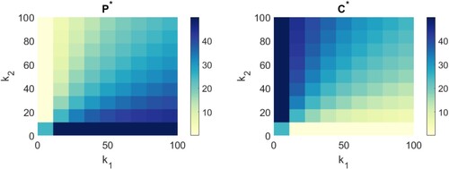
In Figure 2(left), for each $k_1$, $k_2$ pair of values we colour the corresponding square by the value of $P^{\ast }$. Similarly, for Figure 2(right), for each $k_1$, $k_2$ pair of values we colour the corresponding square by the value of $C^{\ast }$. The colorbars provided denote the value of $P^{\ast }$ and $C^{\ast }$ on each plot respectively.

As seen in Figure 2, as the value of $k_1$ increases, the equilibrium value for $P^{\ast }$ increases and the equilibrium value for $C^{\ast }$ decreases and vice versa for $k_2$. We can confirm this analytically by looking at the limits of $C^{\ast }$ and $P^{\ast }$. Take the limit of the equilibrium values as $k_1$ increases to infinity, to determine the long-term value of the number of open and closed channels: $\begin{array}{rl}\underset{k_1\to \mathrm{\infty }}{lim}{C}^{\ast }& =\underset{k_1\to \mathrm{\infty }}{lim}\frac{k_2}{k_1+k_2}N=\underset{k_1\to \mathrm{\infty }}{lim}\frac{\frac{k_2}{k_1}}{1+\frac{k_2}{k_1}}N=\frac{0}{1+0}N=0,\\ \underset{k_1\to \mathrm{\infty }}{lim}{P}^{\ast }& =\underset{k_1\to \mathrm{\infty }}{lim}\frac{k_1}{k_1+k_2}N=\underset{k_1\to \mathrm{\infty }}{lim}\frac{1}{1+\frac{k_2}{k_1}}N=\frac{1}{1+0}N=N.\end{array}$ A similar analysis can be applied to examine the limit as $k_2\to \mathrm{\infty }$ and we suggest this as an exercise. Biologically, this tells us that if we want to increase the number of open channels, we need to increase $k_1$.

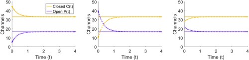
Setting $k_1=1$, $k_2=2$ and N = 50 gives the steady state values of $C^{\ast }=33.3$ and $P^{\ast }=16.7$. Now if we select $C_0=45$ and $P_0=5$, we can simulate the model using a numerical solver of our choice. We choose MATLAB and check that over time $C\left(t\right)$ and $P\left(t\right)$ approach 33.3 and 16.7 respectively, see Figure 3. We see that irrespective of our choice of $C_0$ and $P_0$, over time the number of closed and open ion channels approaches the steady state value $C^{\ast }$ and $P^{\ast }$ that we found in (5(5) $\begin{array}{rl}& C^{\ast }=\frac{k_2}{k_1}(N-C^{\ast }),\\ \Rightarrow & C^{\ast }+\frac{k_2}{k_1}{C}^{\ast }=\frac{k_2}{k_1}N,\\ \Rightarrow & C^{\ast }(1+\frac{k_2}{k_1})=\frac{k_2}{k_1}N,\\ \Rightarrow & C^{\ast }\left(\frac{k_1+k_2}{k_1}\right)=\frac{k_2}{k_1}N,\\ \Rightarrow & C^{\ast }=\frac{k_2}{k_1+k_2}N.\end{array}$(5) )–(6(6) $\Rightarrow P^{\ast }=\frac{k_1}{k_1+k_2}N.$(6) ).

Figure 3. Plot of the numerical solution to (1(1) $\frac{dC}{dt}=-k_{1}C+k_{2}P,$(1) –2(2) $\frac{dP}{dt}=k_{1}C-k_{2}P.$(2) ) against the equilibrium number of closed $C^{\ast }$ and open $P^{\ast }$ ion channels given in (5(5) $\begin{array}{rl}& C^{\ast }=\frac{k_2}{k_1}(N-C^{\ast }),\\ \Rightarrow & C^{\ast }+\frac{k_2}{k_1}{C}^{\ast }=\frac{k_2}{k_1}N,\\ \Rightarrow & C^{\ast }(1+\frac{k_2}{k_1})=\frac{k_2}{k_1}N,\\ \Rightarrow & C^{\ast }\left(\frac{k_1+k_2}{k_1}\right)=\frac{k_2}{k_1}N,\\ \Rightarrow & C^{\ast }=\frac{k_2}{k_1+k_2}N.\end{array}$(5) –6(6) $\Rightarrow P^{\ast }=\frac{k_1}{k_1+k_2}N.$(6) ). The solution to the differential equation is given as a starred line and the steady state value as a straight line. We fixed $k_1=1,k_2=2$ and N = 50 and solved for (left) $C_0=45$, $P_0=5$, (middle) $C_0=10,P_0=40$ and (right) $C_0=28$, $P_0=22$.

To be mathematically rigorous, it is worth noting that there is another steady state value, in other words another choice for $C^{\ast }$ and $P^{\ast }$ so that $dC/dt=dP/dt=0$. If we set $P^{\ast }=0$ and $C^{\ast }=0$ we see that (1(1) $\frac{dC}{dt}=-k_{1}C+k_{2}P,$(1) )–(2(2) $\frac{dP}{dt}=k_{1}C-k_{2}P.$(2) ) becomes $\begin{array}{rl}\frac{dC}{dt}& =-k_1\times 0+k_2\times 0=0,\\ \frac{dP}{dt}& =k_1\times 0-k_2\times 0=0.\end{array}$ However, it is clear from Figure 3, that neither C nor P are tending to zero. Very simply, this can be explained by our original working to determine that $N=C_0+P_0$. As long as $C_0$ and $P_0$ are both non-zero, so initially there is some non-zero number of open and closed ion channels, then N must be positive and constant for all time. As an extension to this, the stability of the two steady states can be proven using undergraduate linear algebra techniques such as matrices, Jacobians, determinants and polynomial roots, however, we leave this as an exercise.

2.3. Solving a system of two ordinary differential equations

Now that we know that the total number of ion channels N is conserved, and we know the long-term steady state value for the number of closed channels $C^{\ast }$ and the number of open channels $P^{\ast }$, a natural next step is to see if we can solve the system of (1(1) $\frac{dC}{dt}=-k_{1}C+k_{2}P,$(1) )–(2(2) $\frac{dP}{dt}=k_{1}C-k_{2}P.$(2) ). Through some algebraic manipulation, differentiation and applying the quadratic formula it is possible to solve this system of equations and this is a great undergraduate exercise. First we differentiate (1(1) $\frac{dC}{dt}=-k_{1}C+k_{2}P,$(1) ): (7) $\begin{array}{rl}& \frac{d}{dt}\left(\frac{dC}{dt}\right)=\frac{d}{dt}(-k_{1}C+k_{2}P),\\ \Rightarrow & \frac{d^{2}C}{d{t}^2}=-k_1\frac{dC}{dt}+k_2\frac{dP}{dt}.\end{array}$(7) then substituting (2(2) $\frac{dP}{dt}=k_{1}C-k_{2}P.$(2) ) into (7(7) $\begin{array}{rl}& \frac{d}{dt}\left(\frac{dC}{dt}\right)=\frac{d}{dt}(-k_{1}C+k_{2}P),\\ \Rightarrow & \frac{d^{2}C}{d{t}^2}=-k_1\frac{dC}{dt}+k_2\frac{dP}{dt}.\end{array}$(7) ) gives (8) $\begin{array}{rl}& \frac{d^{2}C}{d{t}^2}=-k_1\frac{dC}{dt}+k_2(k_{1}C-k_{2}P),\\ \Rightarrow & \frac{d^{2}C}{d{t}^2}=-k_1\frac{dC}{dt}+k_2{k}_{1}C-k_2^{2}P.\end{array}$(8) Now in its current form, (8(8) $\begin{array}{rl}& \frac{d^{2}C}{d{t}^2}=-k_1\frac{dC}{dt}+k_2(k_{1}C-k_{2}P),\\ \Rightarrow & \frac{d^{2}C}{d{t}^2}=-k_1\frac{dC}{dt}+k_2{k}_{1}C-k_2^{2}P.\end{array}$(8) ) still involves P, so before we can attempt to solve this equation, we need to eliminate P. We then rearrange (1(1) $\frac{dC}{dt}=-k_{1}C+k_{2}P,$(1) ) to get an expression for P: (9) $P=\frac{1}{k_2}(\frac{dC}{dt}+k_{1}C).$(9) Taking (9(9) $P=\frac{1}{k_2}(\frac{dC}{dt}+k_{1}C).$(9) ) and substituting in place of P in (8(8) $\begin{array}{rl}& \frac{d^{2}C}{d{t}^2}=-k_1\frac{dC}{dt}+k_2(k_{1}C-k_{2}P),\\ \Rightarrow & \frac{d^{2}C}{d{t}^2}=-k_1\frac{dC}{dt}+k_2{k}_{1}C-k_2^{2}P.\end{array}$(8) ) with some rearranging gives an equation solely in terms of C: (10) $\begin{array}{rl}& \frac{d^{2}C}{d{t}^2}=-k_1\frac{dC}{dt}+k_2{k}_{1}C-k_2^2(\frac{1}{k_2}\frac{dC}{dt}+\frac{k_1}{k_2}C),\\ & \frac{d^{2}C}{d{t}^2}=-k_1\frac{dC}{dt}+k_2{k}_{1}C-k_2\frac{dC}{dt}-k_2{k}_{1}C,\\ & \frac{d^{2}C}{d{t}^2}+k_1\frac{dC}{dt}+k_2\frac{dC}{dt}=0,\\ & \frac{d^{2}C}{d{t}^2}+\frac{dC}{dt}(k_1+k_2)=0.\end{array}$(10) Fortunately, (10(10) $\begin{array}{rl}& \frac{d^{2}C}{d{t}^2}=-k_1\frac{dC}{dt}+k_2{k}_{1}C-k_2^2(\frac{1}{k_2}\frac{dC}{dt}+\frac{k_1}{k_2}C),\\ & \frac{d^{2}C}{d{t}^2}=-k_1\frac{dC}{dt}+k_2{k}_{1}C-k_2\frac{dC}{dt}-k_2{k}_{1}C,\\ & \frac{d^{2}C}{d{t}^2}+k_1\frac{dC}{dt}+k_2\frac{dC}{dt}=0,\\ & \frac{d^{2}C}{d{t}^2}+\frac{dC}{dt}(k_1+k_2)=0.\end{array}$(10) ) is a second order differential equation for C and can be solved using the method of undetermined coefficients, which is an undergraduate technique. This method relies on solving a quadratic equation, something all undergraduates should be familiar with. First, we determine the characteristic equation by replacing $d^{2}C/d{t}^2$ by $y^2$ and $dC/dt$ by y to obtain: (11) $y^2+(k_1+k_2)y=0.$(11) We can then determine the two roots of this quadratic equation, $y_1$ and $y_2$ to give: $\begin{array}{rl}& y^2+(k_1+k_2)y=0,\\ \Rightarrow & y(y+k_1+k_2)=0,\\ \Rightarrow & y_1=0\text{ or }{y}_2+k_1+k_2=0,\\ \Rightarrow & y_2=-(k_1+k_2).\end{array}$ Finally, these roots are used to form the general solution for a second order differential equation: $C\left(t\right)=A{e}^{y_{2}t}+B{e}^{y_{1}t},$ and so we obtain: (12) $C\left(t\right)=A{e}^{-(k_1+k_2)t}+B,$(12) where A and B are integration constants to be determined using the initial conditions $C\left(0\right)=C_0$ and $P\left(0\right)=P_0$. Note that $e^{0t}=1$.

First, we find the solution for $P\left(t\right)$ by substituting the solution for $C\left(t\right)$ into (9(9) $P=\frac{1}{k_2}(\frac{dC}{dt}+k_{1}C).$(9) ): (13) $\begin{array}{rl}P\left(t\right)& =\frac{1}{k_2}(-((k_1+k_2)A{e}^{-(k_1+k_2)t}+k_1(A{e}^{-(k_1+k_2)t}+B)),\\ & =\frac{1}{k_2}(-k_{2}A{e}^{-(k_1+k_2)}+k_{1}B),\\ P\left(t\right)& =-A{e}^{-(k_1+k_2)t}+\frac{k_1}{k_2}B.\end{array}$(13) To solve for A and B we use the initial conditions for C and P, i.e $C\left(0\right)=C_0$ and $P\left(0\right)=P_0$. From (12(12) $C\left(t\right)=A{e}^{-(k_1+k_2)t}+B,$(12) ): $C_0=A+B$ and so $A=C_0-B$. Substituting this into (13(13) $\begin{array}{rl}P\left(t\right)& =\frac{1}{k_2}(-((k_1+k_2)A{e}^{-(k_1+k_2)t}+k_1(A{e}^{-(k_1+k_2)t}+B)),\\ & =\frac{1}{k_2}(-k_{2}A{e}^{-(k_1+k_2)}+k_{1}B),\\ P\left(t\right)& =-A{e}^{-(k_1+k_2)t}+\frac{k_1}{k_2}B.\end{array}$(13) ) gives: $\begin{array}{rl}{P}_0& =-(C_0-B)+\frac{k_1}{k_2}B,\\ P_0& =-C_0+B+\frac{k_1}{k_2}B,\\ P_0+C_0& =B(1+\frac{k_1}{k_2}),\\ B& =\frac{k_2}{k_1+k_2}N.\end{array}$ Substituting in the values for A and B gives the final solutions for $C\left(t\right)$ and $P\left(t\right)$ as (14) $\begin{array}{rl}C\left(t\right)& =(C_0-\frac{k_2}{k_1+k_2}N)e^{-(k_1+k_2)t}+\frac{k_2}{k_1+k_2}N,\end{array}$(14) (15) $\begin{array}{rl}P\left(t\right)& =-(C_0-\frac{k_2}{k_1+k_2}N)e^{-(k_1+k_2)t}+\frac{k_1}{k_1+k_2}N.\end{array}$(15) Bringing our investigations full circle, we can see that as $t\to \mathrm{\infty }$, i.e. as time goes on, both C and P approach the steady state solutions $C^{\ast }$ and $P^{\ast }$ we found earlier, since the exponential terms in (14(14) $\begin{array}{rl}C\left(t\right)& =(C_0-\frac{k_2}{k_1+k_2}N)e^{-(k_1+k_2)t}+\frac{k_2}{k_1+k_2}N,\end{array}$(14) )–(15(15) $\begin{array}{rl}P\left(t\right)& =-(C_0-\frac{k_2}{k_1+k_2}N)e^{-(k_1+k_2)t}+\frac{k_1}{k_1+k_2}N.\end{array}$(15) ) tend to zero. It is also now possible to plot the solution to (1(1) $\frac{dC}{dt}=-k_{1}C+k_{2}P,$(1) )–(2(2) $\frac{dP}{dt}=k_{1}C-k_{2}P.$(2) ) using the formulas in (14(14) $\begin{array}{rl}C\left(t\right)& =(C_0-\frac{k_2}{k_1+k_2}N)e^{-(k_1+k_2)t}+\frac{k_2}{k_1+k_2}N,\end{array}$(14) )–(15(15) $\begin{array}{rl}P\left(t\right)& =-(C_0-\frac{k_2}{k_1+k_2}N)e^{-(k_1+k_2)t}+\frac{k_1}{k_1+k_2}N.\end{array}$(15) ), instead of using a numerical solver.

3. Ion channel modelling in the stochastic setting

So far we have looked at an ODE model for the opening and closing of ion channels. We refer to ODE models as ‘deterministic’, as each time we solve them, the solution is the same (it is ‘determined’). Alternatively, if noise is included in the model (how do we do this?), then each solution is a sample path showing what happens, given the current noise. In one sense, the ODE models provide an averaged solution – for example, how a population is behaving, rather than looking at the behaviour of an individual of that population.

For this application, the ODE model in (1(1) $\frac{dC}{dt}=-k_{1}C+k_{2}P,$(1) )–(2(2) $\frac{dP}{dt}=k_{1}C-k_{2}P.$(2) ) describes the behaviour of a population of ion channels opening and closing. In general, this average behaviour is good enough. If there are a hundred thousand ion channels in the model, then what difference does it make if at a particular time point, C ion channels are closed rather than C−10? But if we want to understand individual channel behaviour and how this manifests at a population level, then we should capture this variability, that is, this stochasticity. For example, neurons are much smaller than cardiac myocytes, so the number of channels on a neuron are much fewer (in the order of thousands) than those on a cardiac myocyte (in the order of hundreds of thousands), and so stochasticity plays an important role. The density or numbers of channels can vary considerably by channel type and location -- see Århem et al. for a discussion on the modelling of channels (Århem et al., 2006).

In the deterministic setting, we can have continuous or discrete models. ODEs are continuous models over time. Similarly for stochastic models – these can be continuous or discrete. In the continuous setting, you would get Stochastic Differential Equations, but it is easier to understand and solve a discrete stochastic model. To do this, we will set up a simple stochastic ion channel model that still captures the total number of open and closed channels, but it evolves in time steps that reflect the waiting time between events; here, the model will have two events

1. closed channel $\to$ open channel

2. open channel $\to$ closed channel.

Stochastic models need to be simulated many times, so that the moments (e.g. the average value, the variance, or higher order moments) can be determined, With multiple simulations, the average solution will approximate the trajectory of the solution of (1(1) $\frac{dC}{dt}=-k_{1}C+k_{2}P,$(1) )–(2(2) $\frac{dP}{dt}=k_{1}C-k_{2}P.$(2) ), and consequently the stochastic solution set allows a richer interpretation (than just the average) of the evolution of the numbers of closed and open channels.

3.1. A simple stochastic ion channel model

Suppose we have a set of time points $0,t_1,t_2,\dots$, and suppose that $C\left(t_i\right)$ is the number of closed channels at time $t_i$, while $P\left(t_i\right)$ is the number of open channels at time $t_i$. In our model we will assume a constant number of channels N, so $C\left(t_i\right)+P\left(t_i\right)=N$ for each time point $t_i$. As in the ODE model, $k_1$ represents the rate at which closed channels open, while $k_2$ is the rate of open channels closing. This is often represented by the following schematic $\begin{array}{r}C\left(t\right)⟹k_{1}P\left(t\right),\\ C\left(t\right)\underset{k_2}{\overset{}{\leftarrow }}P\left(t\right),\end{array}$ which correspond to events (1) and (2) above. We include noise in this model by having a time interval between events $\mathrm{\Delta t}$ that depends on the likelihood of the events, rather than having fixed time intervals. The time between events will be exponentially distributed, and the Worked Example shows you how to simulate this.

At each time point $t_i$, we need to calculate the following quantities: $\begin{array}{rl}{q}_1& =k_{1}C\left(t_i\right),\\ q_2& =k_{2}P\left(t_i\right),\\ r& =q_1+q_2.\end{array}$ As in the ODE example and plot in Figure 1(c), we will take $k_1=1,k_2=2$ and, at the start time $t_0=0,C_0=C\left(0\right)=5$. If we take N = 50, then $P_0=P\left(0\right)=N-C\left(0\right)=45$. We calculate, at the start time $t_0$, $\begin{array}{rl}{q}_1& =k_{1}C\left(t_0\right)=5,\\ q_2& =k_{2}P\left(t_0\right)=90,\end{array}$ and r = 5 + 90 = 95 (at time $t_0$). We can interpret, at this time point, the likelihood of ‘closed $\to$ open’ as having 5 chances out of the total 95, while the likelihood of ‘open $\to$ closed’ is 90 out of 95. We can normalise this as a probability in $[0,1]$ by dividing the number of chances $q_1$ or $q_2$ by the total r.

To simulate the first step, we obtain two random numbers $u_1$ and $u_2$ uniformly distributed on [0,1]. The first random number $u_1$ is used to calculate the waiting time until the next event occurs – this waiting time is exponentially distributed using the parameter r, that is, the waiting time probability density function is given by $P\left(\mathrm{\Delta t}\right)=r\exp (-r\mathrm{\Delta t})$, with associated probability distribution function given by $1-\exp (-r\mathrm{\Delta t}).$ So we calculate the time increment $\mathrm{\Delta t}$ as $\mathrm{\Delta t}=-\frac{1}{r}\log \left(u_1\right).$ (See Section 4 Extension Exercises for an opportunity to derive this expression for $\mathrm{\Delta t}$). Note that by ‘log’ we mean the ‘natural logarithm’ or ${\log }_e$. Then $t_1$, the time that this event occurs, is $t_1=t_0+\mathrm{\Delta t}.$ Now we determine which event occurs, using the second random number $u_2$. The probability of the first event is $q_1/r$, while that of the second event is $q_2/r$. If $u_2<\frac{5}{95}$ (that is, $\frac{q_1}{r}$), then we say that the first option occurs, so a closed channel opens. If $u_2\ge \frac{5}{95}$, then an open channel closes. We have to update the state of the system by adjusting the number of currently closed or open channels according to the value of $u_2$. This completes the first step of the algorithm.

To proceed with the next step, we re-calculate $q_1,q_2$ and r using the current values $C\left(t_1\right)$ and $P\left(t_1\right)$, sample two new random numbers from $U(0,1)$, determine the new value for $\mathrm{\Delta t}$ and then choose whether an ‘open’ or ‘close’ event occurs. Continue in this way while t<T.

The simulation process described above was developed by Gillespie (1977); the evolution over time of a biological system can be represented by ODEs deterministically, or by a stochastic formulation represented by a stochastic master equation that gives the probability of being in a particular system state, for all possible states, at a certain time. However, the stochastic Master Equation is often intractable to calculate for large systems. Gillespie derived the Stochastic Simulation Algorithm (SSA) that numerically simulates the time evolution of the system exactly. You can read more about the SSA and some approaches for reducing computational effort by using a τ-leaping approach in Gillespie (2007).

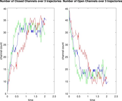
Because we are using different random numbers at each step of the simulation of this model, each solution trajectory will evolve differently (see Figure 4 for three possible solution trajectories). Once many trajectories have been computed, we can build a histogram of the numbers of channels that are open or closed at a particular time. This gives us a richer answer than just the single value we obtained from the ODE model. Our stochastic model and the interpretation of the solution allows the natural variability of when the channels actually open or close to be taken into consideration.

Figure 4. Trajectories showing numbers of closed and open channels (vertical axis) up to time $T=2$ (horizontal axis).

3.2. A worked example

We will now go through several steps of a worked example, so that the algorithm can be clearly understood. We will take the following sequence of uniform random samples, and execute four steps of the algorithm: $\{0.394695,0.685743,0.201421,0.067175,0.553702,0.226967,0.002112\}.$ We will assume the parameters are $k_1=1,k_2=2$, and the initial values are $C\left(0\right)=5,P\left(0\right)=45$ (with total population N = 50).

Step 1

Setting $t_0=0,q_1=k_1\times C\left(0\right)=5$, $q_2=k_2\times P\left(0\right)=45$, and so $r=q_1+q_2=95$. For our first Uniform random sample, we take $u_1=0.394695$ (the first enter in the set above), and compute the time until the next event: $\mathrm{\Delta t}=-\log \left(0.394695\right)/95=0.929641=\mathrm{0.009786.}$ This means that the event occurs at time $t_1=0+\mathrm{\Delta t}=\mathrm{0.009786.}$ To determine which event occurs, we use the next Uniform random sample so $u_2=0.685743$. Is $u_2<\frac{q_1}{r}?$ Now $\frac{q_1}{r}=0.052632$, so the answer is No; consequently, event 2 (Open $\to$ Closed) takes place. We update the system state accordingly. The channel counts become $C\left(t_1\right)=C\left(t_0\right)+1=6,P\left(t_1\right)=P\left(t_0\right)-1=44.$ Step 2

First we recalculate $q_1,q_2$ and r, using the latest channel count values: $q_1=k_1\times C\left(t_1\right)=6,q_2=k_2\times P\left(t_1\right)=88,r=q_1+q_2=94.$ We use the next Uniform random number which is $u_1=0.201421$, and determine that $\mathrm{\Delta t}=-\log \left(0.201421\right)/94=1.602357/94=\mathrm{0.017046.}$ Consequently, the time at which the next event occurs is $t_2=t_1+\mathrm{\Delta t}=0.009786+0.017046=0.026832$. The next Uniform random sample is $u_2=0.067175$. Is $u_2<\frac{q_1}{r}?$ We see that $\frac{q_1}{r}=0.063830$, so the answer is No; consequently, event 2 (Open $\to$ Closed) takes place, and we update the system state accordingly. The channel counts become $C\left(t_2\right)=C\left(t_1\right)+1=7,P\left(t_2\right)=P\left(t_1\right)-1=43.$ Step 3

We recalculate $q_1,q_2$ and r, using the latest channel count values: $q_1=k_1\times C\left(t_2\right)=7,q_2=k_2\times P\left(t_2\right)=86,r=q_1+q_2=93.$ We use the next Uniform random number which is $u_1=0.553702$, and determine that $\mathrm{\Delta t}=-\log \left(0.553702\right)/93=0.591128/93=\mathrm{0.006356.}$ Consequently, the time at which the next event occurs is $t_3=t_2+\mathrm{\Delta t}=0.026832+0.006356=0.033188$. The next Uniform random sample is $u_2=0.226967$. Is $u_2<\frac{q_1}{r}?$ As $\frac{q_1}{r}=0.075269$, the answer is No; consequently, event 2 (Open $\to$ Closed) takes place again, and we update the system state accordingly. The channel counts become $C\left(t_3\right)=C\left(t_2\right)+1=8,P\left(t_3\right)=P\left(t_2\right)-1=42.$ Step 4

We recalculate $q_1,q_2$ and r, using the latest channel count values: $q_1=k_1\times C\left(3\right)=8,q_2=k_2\times P\left(3\right)=84,r=q_1+q_2=92.$ We use the next Uniform random number which is $u_1=0.626170$, and determine that $\mathrm{\Delta t}=-\log \left(0.626170\right)/92=0.468133/92=\mathrm{0.005088.}$ Consequently, the time at which the next event occurs is $t_4=0.033188+0.005088=0.038277$. The next Uniform random sample is $u_2=0.002112$. Is $u_2<\frac{q_1}{r}?$ Now $\frac{q_1}{r}=0.086957$, so the answer is Yes; consequently, event 1 (Closed $\to$ Open) takes place, and we update the system state accordingly. The channel counts become $C\left(t_4\right)=C\left(t_3\right)-1=7,P\left(t_4\right)=P\left(t_3\right)+1=43.$ Table 1 summarises the outcomes from these four steps of the algorithm.

Table 1. Summary of four steps of the algorithm.

Time	Number closed	Number open
0.000000	5	45
0.009786	6	44
0.026832	7	43
0.033188	8	42
0.038277	7	43

 

Comments

• Observe that always $C\left(t_i\right)+P\left(t_i\right)=N=50$.

• Note that, because there are only a few closed channels initially, there is a small likelihood ($<\frac{q_1}{r}$) of a closed channel opening. As the rate of Open channels closing is larger than that of Closed channels opening, the number of closed channels will increase, and in the algorithm, the likelihood $\frac{q_1}{r}$ also increases.

• The time steps are very small. One assumption of the algorithm is that the step size is small enough that one and only one event will take place in that time interval. This makes the simulation very computationally intensive.

• We allow the current trajectory to run for many steps (while t<2), and then we repeat the process for multiple trajectories. With multiple trajectories we will be able to calculate the moments of the variables such as the average value. We will see the number of closed and open channels approaching an equilibrium. For example, Table 2 gives the average number of closed and open channels, simulating while t<2 per trajectory, over a selection of total trajectories:

• When we have simulated a large number of trajectories, it is instructive to look at the total number of Closed or Open channels at or near time T = 2. Figure 5 shows the distribution of the number of closed channels from 1000 trajectories -- the range of values is from 24 to 43 channels, but in most cases (with a standard deviation of 3.27) the number of closed channels is between 32 and 37.

• Figure 6 shows how the stochastic trajectory follows along the same path as the ODE trajectory, while allowing variability in the counts of open and closed channels at finer time-points.

Figure 5. Number of closed channels at T = 2, from 1000 trajectories. The red vertical line represents the number of closed channels (33.26) determined by solving the ODE system (1(1) $\frac{dC}{dt}=-k_{1}C+k_{2}P,$(1) ) and (2(2) $\frac{dP}{dt}=k_{1}C-k_{2}P.$(2) ) using MATLAB's function ode45 and also corresponds to the solution for the steady state value of C* in (5(5) $\begin{array}{rl}& C^{\ast }=\frac{k_2}{k_1}(N-C^{\ast }),\\ \Rightarrow & C^{\ast }+\frac{k_2}{k_1}{C}^{\ast }=\frac{k_2}{k_1}N,\\ \Rightarrow & C^{\ast }(1+\frac{k_2}{k_1})=\frac{k_2}{k_1}N,\\ \Rightarrow & C^{\ast }\left(\frac{k_1+k_2}{k_1}\right)=\frac{k_2}{k_1}N,\\ \Rightarrow & C^{\ast }=\frac{k_2}{k_1+k_2}N.\end{array}$(5) ).

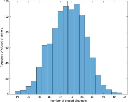
Figure 6. Plot of the solution to the ODE model for ion channels opening and closing in (1(1) $\frac{dC}{dt}=-k_{1}C+k_{2}P,$(1) )–(2(2) $\frac{dP}{dt}=k_{1}C-k_{2}P.$(2) ) with one simulation of Gillespie's Stochastic Simulation Algorithm (SSA) detailed in Section 3.1. We can see that the ODE predicts that C and P will tend smoothly to their steady state values, whereas the SSA will bounce around at the steady state value.

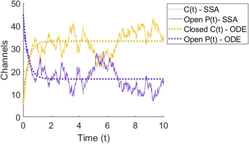
Table 2. Average numbers of closed and open channels.

Number of trajectories	Average number closed	Average number open
20	34.20	15.80
50	32.82	17.18
100	33.29	16.71
200	33.20	16.81
500	33.34	16.66
1000	33.36	16.64

This worked example was for a very simple case where there were only two alternative events. Of course, the algorithm works for multiple events: assume we have four events with associated quantities $q_1,q_2,q_3,q_4$, with $r=q_1+q_2+q_3+q_4$. To determine which of the four events occurs next, we now check in turn as follows: $\begin{array}{rll}\mathrm{if}& u_2<q_1/r& \mathrm{thenEvent}1\mathrm{occurs}\\ \mathrm{elseif}& u_2<(q_1+q_2)/r& \mathrm{thenEvent}2\mathrm{occurs}\\ \mathrm{elseif}& u_2<(q_1+q_2+q_3)/r& \mathrm{thenEvent}3\mathrm{occurs}\\ \mathrm{else}& & \mathrm{Event}4\mathrm{occurs}.\end{array}$

4. Extension exercises

To aid in the teaching of this example, we have provided all code used to generate figures in this manuscript in the Supplementary material and in the GitHub repository https://github.com/AdrianneJennerQUT/modelling-ion-channel-flow. When teaching this course to undergraduate students, we used the opportunity to have them practise good coding skills by uploading any coding files to GitHub and sharing the repository with us for marking. We found that students greatly appreciated the opportunity to learn good coding practices whilst also learning mathematics.

Below, we have provided additional extension exercises and questions that can be used to test student knowledge of the context provided in this example.

1. Consider that the number of open channels on a cell was growing in time. The new model would then be (16) $\begin{array}{rl}\frac{dC}{dt}& =-k_{1}C+k_{2}P,\\ \frac{dP}{dt}& =r+k_{1}C-k_{2}P,\end{array}$(16)

   1. Is the total number of channels still conserved?

   2. How are the total number of channels N changing over time?

   Solution. (a) The total number of channels is no longer conserved, i.e. no longer constant since $dN/dt\ne 0$. (b) $C\left(t\right)+P\left(t\right)=\mathrm{rt}+C_0+P_0$, which says that the number of channels is growing linearly in time.

2. Assume that sodium ions (NA⁺) flow in and out of a cell when the ion channels are open and that $\mathrm{\Phi }\left(t\right)$ is the amount of sodium ions inside a cell. We can model the change in sodium ions within a cell as: (17) $\frac{d\mathrm{\Phi }}{dt}=f_{i}P-f_{o}P\mathrm{\Phi },$(17) where $f_i$ is the rate ions flow in and $f_o$ is the rate ions flow out. What is the steady state value for Φ? Assuming $P^{\ast }$ was given in (6(6) $\Rightarrow P^{\ast }=\frac{k_1}{k_1+k_2}N.$(6) ).

   Solution. ${\mathrm{\Phi }}^{\ast }=f_i/f_o$.

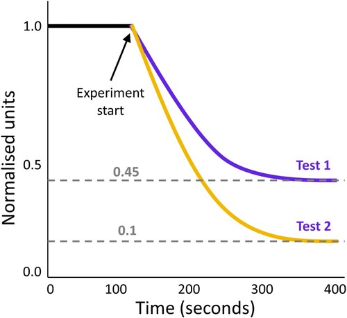
3. An experimentalist measured the number of ion channels closed over time (Figure 7). Given that they knew that $k_1=0.1$, can you determine $k_2$ for both experiments? Data for this question are inspired by the in vitro experiments for potassium ion channel assays (Su et al., 2016).

   Solution. For test 1, $k_2\approx 0.081$ and for test 2 $k_2\approx 0.011$.

4. If the probability distribution function is given by $F\left(\mathrm{\Delta t}\right)=1-\exp (-r\mathrm{\Delta t})$, and if $u\sim U(0,1)$ is uniformly distributed on [0,1], find an expression for $\mathrm{\Delta t}$ so that $u=F\left(\mathrm{\Delta t}\right)$. In other words, find the inverse function $F^{-1}$ where $\mathrm{\Delta t}=F^{-1}\left(u\right)$.

   Solution. Start with $\mathrm{\Delta t}$, multiply by $-r$, take the exponential $\exp$, multiply by -1, and finally add 1. Now do this in reverse from right to left: start with u, subtract 1, divide by -1, take the natural logarithm, divide by $-r$ to get $\mathrm{\Delta t}=-\frac{1}{r}\log (1-u)$. If u is uniformly distributed on [0,1], then so is 1−u.

Figure 7. Fictional experiment for question (3). Data for this figure inspired by the in vitro experiments for potassium ion channel assays (Su et al., 2016).

5. Discussion

In this work, we introduce a system of two ordinary differential equations which model the opening and closing of ion channels on the membrane of a cell. This elegant, yet simple, mathematical model presents an excellent teaching example for a wide range of mathematics students, particularly undergraduates in the first year of study. We show how fundamental techniques such as algebraic manipulation, differentiation, substitution, rearrangement and integration all allow us to understand the dynamics of this model and hence the biological system it captures. Furthermore, we show how Gillespie's Stochastic Simulation Algorithm can be used to simulate noise in this biological system, again drawing on an undergraduate understanding of random numbers, the Uniform distribution and the natural log.

The worked examples here have been presented so that they can be recreated in the classroom. For students in differential calculus courses, steady state solutions are a typical learning outcome for these courses. Furthermore, while not demonstrated here, this system can be used in linear algebra courses to demonstrate how to construct a system of ODEs from a vector $\overrightarrow{X}=[C,P{]}^T$ with matrix A as the coefficients of the exponents in each equation, i.e. $\frac{d}{dt}\overrightarrow{X}=\left[\begin{array}{cc}-k_1& k_2\\ k_1& -k_2\end{array}\right]\overrightarrow{X}.$ In addition, solving systems of ODEs by converting them to a second order differential equation is a fundamental part of calculus of one variable and is often taught in first year undergraduate classes. Lastly, most students have seen limits before entering University, however, in abstract concepts. In this article, we provide applications of limits to real-world examples as well as use limits to answer biologically motivated questions.

Our experience teaching the content of this paper has been in a mathematical modelling unit aimed at science graduates (non-mathematicians). In this unit, the goal is to teach ways in which differential equation models can capture the real-world. We have found that having tangible real examples for students, such as the ion channel model, has significantly increased their understanding of mathematics and their confidence to tackle mathematical questions. We also find that while the Stochastic Simulation Algorithm can feel advanced initially, students take to it well for it is at its core, formula evaluation. In addition, the SSA presents a nice opportunity to examine a student's ability to plot data. This can be achieved, by asking a student to plot their solution for C and P (such as the values in Table 1) which they could obtain by hand in an exam.

In conclusion, a real-world application example (such as the one in this paper) provides an opportunity for students to develop their analytical skills in differential equations, resulting in a deeper understanding of the connections between the differential equations and the application example. While the system in (1(1) $\frac{dC}{dt}=-k_{1}C+k_{2}P,$(1) )–(2(2) $\frac{dP}{dt}=k_{1}C-k_{2}P.$(2) ) was presented as motivated by the ion channel biology, this simple system can represent many other biological phenomena, such as chemical signalling networks or the movement of cells from the blood into an organ and we highly recommend the application of this example to contexts that may be relevant for the undergraduates taking the course.

Disclosure statement

No potential conflict of interest was reported by the authors.

References

- Århem, P., Klement, G., & Blomberg, C. (2006). Channel density regulation of firing patterns in a cortical neuron model. Biophysical Journal, 90(12), 4392–4404. https://doi.org/10.1529/biophysj.105.077032
- Bartos, D. C., Grandi, E., & Ripplinger, C. M. (2015). Ion channels in the heart. Comprehensive Physiology, 5(3), 1423. https://doi.org/10.1002/cphy
- Beier, J. C., Gevertz, J. L., & Howard, K. E. (2015). Building context with tumor growth modeling projects in differential equations. PRIMUS, 25(4), 297–325. https://doi.org/10.1080/10511970.2014.975881
- da Silva Soares, D., & Borba, M. C. (2014). The role of software modellus in a teaching approach based on model analysis. ZDM, 46, 575–587. https://doi.org/10.1007/s11858-013-0568-5
- Gillespie, D. T. (1977). Exact stochastic simulation of coupled chemical reactions. The Journal of Physical Chemistry, 81(25), 2340–2361. https://doi.org/10.1021/j100540a008
- Gillespie, D. T. (2007). Stochastic simulation of chemical kinetics. Annual Review of Physical Chemistry, 58, 35–55. https://doi.org/10.1146/physchem.2007.58.issue-1
- González-Martín, A. S., Gueudet, G., Barquero, B., & Romo-Vázquez, A. (2021). Mathematics and other disciplines, and the role of modelling: Advances and challenges. Research and Development in University Mathematics Education, 169–189.
- Gravemeijer, K., & Doorman, M. (1999). Context problems in realistic mathematics education: A calculus course as an example. Educational Studies in Mathematics, 39(1–3), 111–129. https://doi.org/10.1023/A:1003749919816
- Khotimah, R. P., & Masduki, M. (2016). Improving teaching quality and problem solving ability through contextual teaching and learning in differential equations: A lesson study approach. JRAMathEdu (Journal of Research and Advances in Mathematics Education), 1(1), 1–13. https://doi.org/10.23917/jramathedu.v1i1.1791
- Kwon, O. N., Rasmussen, C., & & Allen, K. (2016). Students' retention of mathematical knowledge and skills in differential equations. School Science and Mathematics, 105(5), 227–239. https://doi.org/10.1111/j.1949-8594.2005.tb18163.x
- McCarthy, C., Swanson, E., & & Winkeln, B. (2019). Special issue of PRIMUS: Modeling approach to teaching differential equations. PRIMUS, 29(6), 503–508. https://doi.org/10.1080/10511970.2019.1565789
- Nelson, M. I. (2023). How long should a town be locked down to eliminate an infectious disease?. International Journal of Mathematical Education in Science and Technology, 54(6), 1–15.
- Pathmanathan, P., & Gray, R. A. (2018). Validation and trustworthiness of multiscale models of cardiac electrophysiology. Frontiers in Physiology, 9, 106. https://doi.org/10.3389/fphys.2018.00106
- Seshaiyer, P., & Lenhart, S. (2020). Connecting with teachers through modeling in mathematical biology. Bulletin of Mathematical Biology, 82(8), 1–18. https://doi.org/10.1007/s11538-020-00774-3
- Su, Z., Brown, E. C., Wang, W., & MacKinnon, R. (2016). Novel cell-free high-throughput screening method for pharmacological tools targeting K+ channels. Proceedings of the National Academy of Sciences, 113(20), 5748–5753. https://doi.org/10.1073/pnas.1602815113
- Tang, Y., & Wang, F. (2010). Ion channel modeling and simulation using hybrid functional Petri net. In Life system modeling and intelligent computing: International conference on life system modeling and simulation, LSMS 2010, and international conference on intelligent computing for sustainable energy and environment, ICSEE 2010, Wuxi, China, September 17–20, 2010. Proceedings, Part III (pp. 404–412).