Proof of the small angle approximation sinθ≈θ using the geometry and motion of a simple pendulum

Abstract

The small angle approximation $\text{sin}(\theta )\approx \theta$ is central to all treatments of the simple pendulum as a harmonic oscillator and is typically asserted as a result that follows from calculus. Here, however, we show that the geometry of the pendulum itself offers a route to understanding the origin of the small angle approximation without recourse to calculus. Rather charmingly, our approach exploits the motion of the pendulum to visualise the process of taking an important limit and can be used to explore the meaning of mathematical approximation in physical systems.

KEYWORDS:

• Simple harmonic motion
• simple pendulum
• limits
• linearisation
• small angle approximation
• methods of approximation

1. Introduction

Central to all treatments of the simple pendulum as a harmonic oscillator is the requirement that the pendulum’s angle of displacement $\theta$ (measured in radians) must be ‘small’. Indeed, if this is the case then one may make the small angle approximation (1) $\text{sin}(\theta )\approx \theta ,$(1) and thence show that the restoring force on the bob (the mass at the end of the pendulum¹) is opposite and proportional to its displacement, i.e. harmonic (Baker & Blackburn, 2005; Richardson & Brittle, 2012; Serway & Vuille, 2006; Tisdell, 2019a). In high-school (pre-calculus) level physics, this approximation is typically motivated informally using trial values or sketching curves, whereas at introductory undergraduate level one may appeal to a linearised Taylor series for $\text{sin}(\theta )$ (Riley et al., 2006). In either case, however, the small angle approximation is asserted as a mathematical result that may be used to understand the behaviour of the pendulum, i.e. as mathematics applied to physics (see Section 2).

In this article, however, we turn the standard argument on its head by showing how the geometry and motion of the simple pendulum itself can be used to understand the origin and meaning of small angle approximation (i.e., we apply physics to mathematics). At the heart of our discussion is an elementary, i.e. ‘non-calculus’ proof for the limiting value of $\text{sin}(\theta )/\theta$, as $\theta \to 0$ (see Section 3). From a teaching perspective, therefore, our approach can be used in at least three different ways, dependent on context. First, for high-school level physics, our method justifies the small angle approximation without recourse to calculus (a justification currently absent from the standard introductory physics literature (Serway & Vuille, 2006)). Second, for classes on calculus, our analysis capitalises on the physical motion of the pendulum to illustrate the process of taking an important limit. Third, for introductions to mathematical modelling, our argument elucidates the meaning of the small angle approximation when applied to physical systems (see Section 4).

Ultimately, of course, our approach can also be viewed simply as a neat didactic exercise, one which connects key concepts in physics with those in mathematics, especially calculus (Soares & Caramelo, 2015; Soares & Morgado, 2022), and encourages multiple perspectives on the small angle approximation suitable for a diverse range of learning styles (Stupel & Ben-Chaim, 2017; Tisdell, 2018; Tisdell, 2019b). Indeed, although our argument is closely related to conventional proofs for the limiting value of $\text{sin}(\theta )/\theta$ as $\theta \to 0$ (Gilbert & Jordan, 2002; Stroud & Booth, 2020), our geometry exploits the motion of the pendulum as a powerful visual aid (Haciomeroglu & Chicken, 2019).

2. Why the approximation is needed

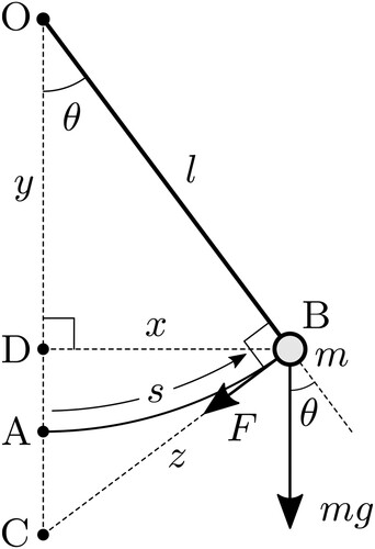
Let us first review why the small angle approximation is needed by summarising the standard ‘non-calculus’ approach to analysing pendulum motion (Serway & Vuille, 2006). To this end, consider the simple pendulum of length $l$ and bob mass $m$ depicted in Figure 1. In this figure, the pendulum is attached to a point O such that the line of the pendulum OB makes an angle $\theta$ with the vertical OC, and the pendulum swings through an arc AB of length (2) $s=l\theta .$(2) Since the weight of the bob is $mg$, where $g$ is the acceleration due to gravity, the restoring force $F$ along the arc (i.e. at right angles to the pendulum) is (3) $F=mg\text{sin}(\theta ).$(3) Thus if we denote $a=-(F/m)$ as the acceleration of the bob along the arc, then (4) $a=-g\text{sin}(\theta )=-g\left(\frac{\text{sin}(\theta )}{l\theta }\right)l\theta =-\left(\frac{g}{l}\right)\left(\frac{\text{sin}(\theta )}{\theta }\right)s,$(4) where we used the fact that $s=l\theta$.² It therefore follows that if one is justified in making the approximation $\text{sin}(\theta )/\theta \approx 1$, then the acceleration will take the harmonic form (5) $a\approx -{\omega }^{2}s,\text{with }\omega =\sqrt{\frac{g}{l}}$(5) as the frequency of oscillation (Serway & Vuille, 2006).

Figure 1. Pendulum OB of length $l$ and bob mass $m$, swinging through an angle $\theta$, along an arc AB of length $s=l\theta$. The weight of the bob is $mg$, such that the restoring force $F$ along the arc (i.e. at right angles to the pendulum) is $F=mg\text{sin}(\theta )$.

3. Proof of the approximation

According to Equations (4) and (5), the motion of the pendulum is harmonic only when $\text{sin}(\theta )/\theta \approx 1$. Typically this result is demonstrated using Taylor series assuming $\theta$ to be sufficiently small (hence small angle approximation). Rather than appeal to results from calculus, however, here we shall show how and when the approximation $\text{sin}(\theta )/\theta \approx 1$ is justified using the geometry of the pendulum itself.

To this end, observe from Figure 1 that if $x$ is the bob’s horizontal displacement (DB), if $y$ is the bob’s vertical displacement (OD), and if $z$ is the bob's displacement along the line CB perpendicular to OB, then (6) $x=l\text{sin}(\theta ),y=l\text{cos}(\theta ),\text{and}z=l\text{tan}(\theta )=l\frac{\text{sin}(\theta )}{\text{cos}(\theta )}.$(6) In this way, the area $A_{\text{S}}$ of the small triangle ODB and the area of area $A_{\text{L}}$ of the large triangle OBC are respectively (7) $A_{\text{S}}=\frac{1}{2}xy=\frac{1}{2}{l}^2\text{sin}(\theta )\text{cos}(\theta ),\text{and}{A}_{\text{L}}=\frac{1}{2}zl=\frac{1}{2}{l}^2\frac{\text{sin}(\theta )}{\text{cos}(\theta )}.$(7) The origin of the small angle approximation may then be understood by comparing these areas with the area $A$ of the pendulum’s circular sector OAB, namely (8) $A=\left(\frac{\theta }{2\pi }\right)\pi l^2=\frac{1}{2}\theta l^2.$(8) Indeed, since the area of the circular sector OAB is larger than that of the small triangle ADB, i.e. $A_{\text{S}}\le A$, we have (9) $\frac{1}{2}{l}^2\text{sin}(\theta )\text{cos}(\theta )\le \frac{1}{2}\theta l^2,\text{that is},\frac{\text{sin}(\theta )}{\theta }\le \frac{1}{\text{cos}(\theta )}.$(9) Similarly, since the area of the circular sector OAB is smaller than that of the large triangle OBC, i.e. $A\le A_{\text{L}}$, we have (10) $\frac{1}{2}\theta l^2\le \frac{1}{2}{l}^2\frac{\text{sin}(\theta )}{\text{cos}(\theta )},\text{that is},\text{cos}(\theta )\le \frac{\text{sin}(\theta )}{\theta }.$(10) Hence, combining inequalities (9) and (10), we obtain (11) $\text{cos}(\theta )\le \frac{\text{sin}(\theta )}{\theta }\le \frac{1}{\text{cos}(\theta )}.$(11) Inequality (11) is valid for all angles in the range $0<\theta <\pi /2$ and provides lower and upper bounds on the value of $\text{sin}(\theta )/\theta$. To see how this leads us to the small angle approximation, therefore, we now investigate what happens as $\theta$ gets vanishingly close to $0$, that is, we consider the limit as $\theta \to 0$, i.e. (12) $\underset{\theta \to 0}{lim}\text{cos}(\theta )\le \underset{\theta \to 0}{\text{lim}}\left(\frac{\text{sin}(\theta )}{\theta }\right)\le \underset{\theta \to 0}{\text{lim}}\left(\frac{1}{\text{cos}(\theta )}\right).$(12) Strictly speaking, the process of evaluating the limits in Equation (12) requires results from pure mathematics (i.e. analysis) (Gilbert & Jordan, 2002); however, for classes in science and engineering, we can use the motion of the pendulum as an informal way of understanding how the limits work. In particular, according to Figure 1, the limit $\theta \to 0$ may be visualised by supposing that the pendulum moves along the arc AB until the arc-length $s$ vanishes ($s\to 0$). In this way, $\theta \to 0$ means that $y\to l$, and thus (13) $\underset{\theta \to 0}{lim}\text{cos}(\theta )=\underset{y\to l}{\text{lim}}\left(\frac{y}{l}\right)=1,\text{and}\underset{\theta \to 0}{lim}\left(\frac{1}{\text{cos}(\theta )}\right)=\underset{y\to l}{\text{lim}}\left(\frac{l}{y}\right)=1.$(13) Hence, putting these expressions into inequality (12), we obtain (14) $1\le \underset{\theta \to 0}{\text{lim}}\left(\frac{\text{sin}(\theta )}{\theta }\right)\le 1,\text{i}\text{.e}\text{., }\underset{\theta \to 0}{\text{lim}}\left(\frac{\text{sin}(\theta )}{\theta }\right)=1.$(14) Informally, the meaning of this limit is that $sin(\theta )/\theta$ can be made as close as we like to $1$ provided that we make $\theta$ sufficiently ‘close to zero’ (Gilbert & Jordan, 2002). It follows from this limit that provided $\theta$ is sufficiently ‘close to zero’ then (15) $\frac{\text{sin}(\theta )}{\theta }\approx 1,\text{or }\text{sin}(\theta )\approx \theta ;$(15) this is the small angle approximation as desired, which is exact if $\theta =0$.

4. How small is ‘small’?

Our discussion above gives a ‘non-calculus’ justification for using the approximation $\text{sin}(\theta )/\theta \approx 1$ provided that $\theta$ is sufficiently ‘close to zero’. Since magnitude comparisons with zero are difficult to define in physical systems, scientists and engineers typically express the concept of $\theta$ being sufficiently ‘close to zero’ as the requirement that $\theta$ must be ‘small’, where ‘small’ means ‘much less than 1’. This idea may be indicated explicitly in the pendulum’s governing Equation (5) by writing (16) $a\approx -{\omega }^{2}s,\text{for}\theta \ll 1.$(16) Since $\theta =s/l$, the pendulum’s motion may therefore be modelled as harmonic only if the amplitude of oscillation is ‘much less’ than the pendulum’s length, i.e. (17) $s/l\ll 1,\text{or }x/l\ll 1,$(17) where the latter inequality follows because $x<s$ (see Figure 1). From a modelling perspective, then the question we must ask ourselves is how much less?

To answer this question, let us again appeal to our geometric argument by using the fact that $y=\sqrt{l^2-x^2}$ to write $\text{cos}(\theta )=y/l=\sqrt{1-{(x/l)}^2}$, and thereby express inequality (11) as (18) $\sqrt{1-{(x/l)}^2}\le \frac{\text{sin}(\theta )}{\theta }\le \frac{1}{\sqrt{1-{(x/l)}^2}}.$(18) Since this inequality gives lower and upper bounds on the value of $\text{sin}(\theta )/\theta$, it is clear that, as $x/l$ gets smaller, $\text{sin}(\theta )/\theta$ gets closer to 1, that is, the approximation $\text{sin}(\theta )/\theta \approx 1$ gets better. This fact emphasises an important point about how mathematical approximation works in physical systems: the small angle approximation is not something to be considered right or wrong; it is a modelling assumption to be considered more or less accurate (see Table 1) (Rivera-Figueroa & Lima-Zempoalteca, 2021).

Table 1. Increasing accuracy of the small angle approximation $\text{sin}(\theta )/\theta \approx 1$ as $x/l$ gets smaller, and $\sqrt{1-{(x/l)}^2}=\text{cos}(\theta )$ approaches 1 (cf. inequalities (11) and (18)).

$x/l$	$\sqrt{1-{(x/l)}^2}$	$\le$	$\text{sin}(\theta )/\theta$	$\le$	1/$\sqrt{1-{(x/l)}^2}$
0.01000	0.99995	$\le$	0.99998	$\le$	1.00005
0.02000	0.99980	$\le$	0.99993	$\le$	1.00020
0.02500	0.99969	$\le$	0.99990	$\le$	1.00031
0.05000	0.99875	$\le$	0.99958	$\le$	1.00125
0.10000	0.99499	$\le$	0.99833	$\le$	1.00504
0.20000	0.97980	$\le$	0.99335	$\le$	1.02062
0.25000	0.96825	$\le$	0.98962	$\le$	1.03280
0.50000	0.86603	$\le$	0.95885	$\le$	1.15470

Table 1 illustrates this idea by listing example values of $\text{sin}(\theta )/\theta$ for various $x/l$. Note that if $x/l<0.25$, then the approximation $\text{sin}(\theta )/\theta \approx 1$ is accurate to better than 1%; this value corresponds to $\theta \approx 0.253$ radians, or about ${14.5}^{\circ }$, which may be why some authors assert $\theta <{15}^{\circ }$ as a condition for the approximation to apply (Serway & Vuille, 2006). Nevertheless, while stating simple ‘cut-off’ conditions of this kind might seem appealing when answering students’ queries, it risks masking the importance of critical thinking about when modelling assumptions are appropriate. Indeed, there are at least three reasons why such thinking is important. First, the validity of an approximation depends on context: for instance, 1% accuracy in the approximation $\text{sin}(\theta )\approx \theta$ may not be sufficient if one requires an overall modelling accuracy of greater than 1% (see, e.g. Rivera-Figueroa and Lima-Zempoalteca 2021). Second, a mathematical model is typically only as good as its weakest assumption; indeed, the simple pendulum model assumes negligible air resistance and a point-mass bob, both of which may be weaker assumptions than $\text{sin}(\theta )\approx \theta$ in some contexts. Third, as discussed by Rivera-Figueroa and Lima-Zempoalteca (2021), ensuring accuracy in the linear approximation for the differential equation governing the simple pendulum is not necessarily the same thing as ensuring accuracy in the equation’s solution (especially when evaluating the pendulum’s time period $T=2\pi \sqrt{l/g}$).

5. Summary

The small angle approximation $\text{sin}(\theta )\approx \theta$ is central to all treatments of the simple pendulum as a harmonic oscillator (Section 2) and is ubiquitous throughout physics. Whilst this result is typically motivated by appealing to a linearised Taylor series for $\text{sin}(\theta )$, here we have shown that the approximation may be understood using the geometry and motion of the pendulum itself. Our analysis is likely to be of interest to physics teachers seeking an elementary (i.e. ‘non-calculus’) justification for why $\text{sin}(\theta )\approx \theta$ when $\theta$ is small and provides a neat visual strategy for evaluating the historically important limit (19) $\underset{\theta \to 0}{\text{lim}}\left(\frac{\text{sin}(\theta )}{\theta }\right)=1$(19) that is applicable to classes on introductory calculus (Section 3). Furthermore, by providing lower and upper bounds on the value of $\text{sin}(\theta )/\theta$, our geometric approach clarifies the concept of approximation as a process of making modelling assumptions which are considered more or less accurate (rather than right or wrong, see Section 4), and can help prepare students for other applications of mathematical linearisation encountered elsewhere in undergraduate study.

Disclosure statement

No potential conflict of interest was reported by the author.

Notes

1 For example, a clock pendulum is typically constructed by attaching a large mass (or ‘bob’) to the end of a thin, stiff rod.

2 Note that if calculus is permitted, then we have $a=\ddot{s}=l\ddot{\theta }$, such that Equation (2.3) may be written as $\ddot{\theta }=-(g/l)\text{sin}(\theta )$, which is the conventional differential equation for pendulum dynamics (Baker & Blackburn, 2005).

References

- Baker, G. L., & Blackburn, J. A. (2005). The pendulum: A case study in physics. Oxford University Press.
- Gilbert, J., & Jordan, C. (2002). Mathematical methods (2nd Edition). Palgrave Macmillan.
- Haciomeroglu, E. S., & Chicken, E. (2019). Visual thinking and gender differences in high school calculus. International Journal of Mathematical Education in Science and Technology, 43(3), 303–313. https://doi.org/10.1080/0020739X.2011.618550
- Richardson, T. H., & Brittle, S. A. (2012). Physical pendulum experiments to enhance the understanding of moments of inertia and simple harmonic motion. Physics Education, 47(5), 537–544. https://doi.org/10.1088/0031-9120/47/5/537
- Riley, K. F., Hobson, M. P., & Bence, S. J. (2006). Mathematical methods for physics and engineering (3rd Edition). Cambridge University Press.
- Rivera-Figueroa, A., & Lima-Zempoalteca, I. (2021). Motion of a simple pendulum: A digital technology approach. International Journal of Mathematical Education in Science and Technology, 52(4), 550–564. https://doi.org/10.1080/0020739X.2019.1692934
- Serway, R. A., & Vuille, C. (2006). College physics (9th Edition). Cengage Learning.
- Soares, A. A., & Caramelo, L. (2015). Using infinite series to calculate the centre of mass of triangular plates. International Journal of Mathematical Education in Science and Technology, 46(6), 916–921. https://doi.org/10.1080/0020739X.2015.1011245
- Soares, A. A., & Morgado, L. (2022). Calculating the centre of mass of circular sector plates using series and limits. International Journal of Mathematical Education in Science and Technology, 46(6), 3176–3183. https://doi.org/10.1080/0020739X.2021.1966530
- Stroud, K. A., & Booth, D. J. (2020). Engineering mathematics (8th Edition). Macmillan International.
- Stupel, M., & Ben-Chaim, D. (2017). Using multiple solutions to mathematical problems to develop pedagogical and mathematical thinking: A case study in a teacher education program. Investigations in Mathematics Learning, 9(2), 86–108. https://doi.org/10.1080/19477503.2017.1283179
- Tisdell, C. C. (2018). Pedagogical alternatives for triple integrals: Moving towards more inclusive and personalized learning. International Journal of Mathematical Education in Science and Technology, 49(5), 792–801. https://doi.org/10.1080/0020739X.2017.1408150
- Tisdell, C. C. (2019a). An accessible, justifiable and transferable pedagogical approach for the differential equations of simple harmonic motion. International Journal of Mathematical Education in Science and Technology, 50(6), 950–959. https://doi.org/10.1080/0020739X.2018.1516826
- Tisdell, C. C. (2019b). On Picard's iteration method to solve differential equations and a pedagogical space for otherness. International Journal of Mathematical Education in Science and Technology, 50(5), 788–799. https://doi.org/10.1080/0020739X.2018.1507051