Modelling the evolution of human postmenopausal longevity using ordinary differential equations

Abstract

We present two simple ODE systems based on the mathematical model in Le et al. (2022) investigating how human postmenopausal longevity could have evolved. Specifically, our ODE systems address a fairly recent and provocative hypothesis that ancestral males choosing younger mates drove the evolution of menopause (Morton et al., 2013).

We analyse one system in two ways: (1) determining the explicit solution and (2) reducing it to one ODE and drawing a bifurcation diagram. We analyse the other system by reducing it to two ODEs and using a phase plane. The concepts in this article are suitable for a late second-year or third-year course in nonlinear ODEs.

Our models demonstrate that undergraduate students of dynamical systems can critically engage with a highly cited and internationally recognised hypothesis of human evolution.

Keywords:

• Ordinary differential equations
• mathematical modelling
• human evolution
• menopause
• mating

1. Introduction

A notable difference between humans and other great apes is women often live well past their end of fertility (Blurton Jones et al., 2002). Why did human postmenopausal lifespans evolve? In 2013, a provocative theory gained traction–the male mate-choice hypothesis (Morton et al., 2013)–and was featured in the BBC online article ‘Men “to blame for the menopause” ’ (Parkinson, 2013).

For their hypothesis, Morton et al. (2013) propose that ancestral males developed a mating preference for younger females leaving older females without offspring, causing old-age female fertility to decline due to the accumulation of deleterious mutations that were no longer counterbalanced by natural selection. Needless to say, the hypothesis generated much controversy, some of which is summarised in Saini (2017).

In their study, Morton et al. developed an agent-based model (ABM) to support their proposition, and as with many ABMs, their model is complex and computationally demanding. Fortunately, the male mate-choice hypothesis proves amendable to investigating using systems of ordinary differential equations (ODEs), which we do here.

We will consider two simple ODE systems based on the larger model of Le et al. (2022) and provide exercises suitable for late second-year or third-year undergraduate courses in nonlinear ODEs. The exercises include calculating the explicit solution of a 2-D linear ODE system, drawing the bifurcation diagram of a 1-D ODE, and drawing the phase plane of a 2-D nonlinear ODE system. We explain model formulations to assist students in understanding their constructions but do not focus on teaching the principles of modelling. Conveying the art of modelling would probably best occur in a project-based setting through dialogue between a supervisor and student or group of students and is not the focus of this article.

In Section 2, we present a female-only model with mutating end of female fertility, leading to a 2-D ODE system, which we analyse first by explicitly solving it and alternatively by reducing it to one ODE and plotting a bifurcation diagram. In Section 3, we develop a two-sex model with mutating end of female fertility and male mating preference, leading to a 4-D ODE system, which we reduce to two dimensions and analyse using a phase plane. Through these exercises, we will find that the male mate-choice hypothesis only holds in the unlikely scenario that ancestral males hardly ever mated with older females. Our analysis will show that even a slight chance of mating with an older female or a small subpopulation of less choosy males will produce enough selection pressure to maintain female fertility into old age.

2. Female-only model with mutating end of female fertility

From experience, one of the most difficult transitions from applying classroom material to real-world problems in another field is translating it into a mathematical expression that can be easily manipulated and analysed to form valid conclusions. In the context of the current problem, we first must identify key features that we would like to capture. As menopause affects only women, we can simplify the problem by initially building a single-sex, female-only model. Also, we focus on the most notable traits in the hypothesis, old-age female infertility and male mating preferences.

2.1. Model

Populations: Let us consider two populations, females with trait 1 $(F_1)$ and females with trait 2 $(F_2)$. Trait 1 represents lifelong fertility, and trait 2 represents a deleterious mutation causing a decline in fertility at older ages. The populations are shown in the black circles in Figure 1.

Figure 1. Diagram of female-only model (1(1) $\begin{array}{rl}\frac{\mathrm{d}{F}_1}{\mathrm{d}t}& =\underset{\begin{array}{c}\mathrm{Offspring}\mathrm{produced}\mathrm{by}\\ \mathrm{young}\mathrm{and}\mathrm{old}{F}_1\\ \mathrm{females}\mathrm{with}\mathrm{no}\mathrm{mutation}\end{array}}{\underbrace{(1-\epsilon )(a+\mathrm{\gamma b})F_1}}-\underset{\mathrm{Death}}{\underbrace{\delta F_1}},\end{array}$(1) )–(2(2) $\begin{array}{rl}\frac{\mathrm{d}{F}_2}{\mathrm{d}t}& =\underset{\begin{array}{c}\mathrm{Offspring}\mathrm{produced}\mathrm{by}\\ \mathrm{young}\mathrm{and}\mathrm{old}{F}_1\\ \mathrm{females}\mathrm{with}\mathrm{mutation}\end{array}}{\underbrace{\epsilon (a+\mathrm{\gamma b})F_1}}+\underset{\begin{array}{c}\mathrm{Offspring}\mathrm{produced}\\ \mathrm{by}\mathrm{young}{F}_2\mathrm{females}\end{array}}{\underbrace{a{F}_2}}-\underset{\mathrm{Death}}{\underbrace{\delta F_2}},\end{array}$(2) ).

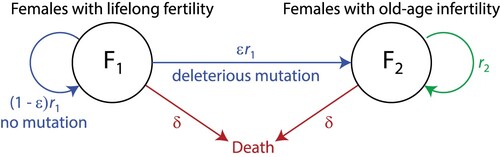
Reproduction and mutation:

We assume females in $F_1$ and $F_2$ reproduce at rates $r_1$ and $r_2$, respectively. Like Morton et al., we assume mutations occur in one direction: lifelong fertility (trait 1) to old-age infertility (trait 2) (Morton et al., 2013). Every time a female in $F_1$ reproduces at rate $r_1$, she has a probability ε of producing an offspring with the deleterious mutation and a probability of $1-\epsilon$ of producing an offspring with the original trait, shown by the blue arrows in Figure 1. Females in $F_2$ reproduce at rate $r_2$ and all their offspring remain in the $F_2$ population, shown by the green arrow.

Death: We assume all individuals die at the same rate δ, shown by the red arrows in Figure 1.

Age classes, mating, and reproductive rates: We do not explicitly model the transition of individuals through different age classes; however, we still need to differentiate between young and old females. We define young, sexually mature females as those between ages 15 to 45 and old females as those over age 45. Hence, the age 45 represents an approximate midlife transition point.

For simplicity, we assume the populations exist at stable age distributions, meaning the proportions in each age class remain constant over time. Let ${\psi }_a$ and ${\psi }_b$ be the proportions of young and old females, and let β be the average rate fertile females produce daughters. Then, in population $F_1$ with lifelong fertility, young and old females reproduce at rates $a{F}_1$ and $b{F}_1$ respectively, assuming they can all find mates, where $a=\beta {\psi }_a$ and $b=\beta {\psi }_b$. In population $F_2$ with old-age infertility, young females reproduce at rate $a{F}_2$ and old females do not reproduce.

To model male mating preference, we follow the assumption of Morton et al. that males always desire to mate with young females from both the $F_1$ and $F_2$ populations, so a young female who is ready to conceive finds a mate with probability 1. On the other hand, males have less desire to mate with old females, so the probability an old female finds a mate is $\gamma \le 1$. Hence, for population $F_1$, the total reproduction rate is $r_1=a+\mathrm{\gamma b}$, which is the sum of the reproductive contribution of young females and old females who are able to find mates. For population $F_2$, only young females can reproduce, so the reproduction rate is $r_2=a$.

Putting these pieces together, we arrive at the ODE system (1) $\begin{array}{rl}\frac{\mathrm{d}{F}_1}{\mathrm{d}t}& =\underset{\begin{array}{c}\mathrm{Offspring}\mathrm{produced}\mathrm{by}\\ \mathrm{young}\mathrm{and}\mathrm{old}{F}_1\\ \mathrm{females}\mathrm{with}\mathrm{no}\mathrm{mutation}\end{array}}{\underbrace{(1-\epsilon )(a+\mathrm{\gamma b})F_1}}-\underset{\mathrm{Death}}{\underbrace{\delta F_1}},\end{array}$(1) (2) $\begin{array}{rl}\frac{\mathrm{d}{F}_2}{\mathrm{d}t}& =\underset{\begin{array}{c}\mathrm{Offspring}\mathrm{produced}\mathrm{by}\\ \mathrm{young}\mathrm{and}\mathrm{old}{F}_1\\ \mathrm{females}\mathrm{with}\mathrm{mutation}\end{array}}{\underbrace{\epsilon (a+\mathrm{\gamma b})F_1}}+\underset{\begin{array}{c}\mathrm{Offspring}\mathrm{produced}\\ \mathrm{by}\mathrm{young}{F}_2\mathrm{females}\end{array}}{\underbrace{a{F}_2}}-\underset{\mathrm{Death}}{\underbrace{\delta F_2}},\end{array}$(2) where parameter definitions are summarised in Table 1.

Table 1. Parameters and variables for (1(1) $\begin{array}{rl}\frac{\mathrm{d}{F}_1}{\mathrm{d}t}& =\underset{\begin{array}{c}\mathrm{Offspring}\mathrm{produced}\mathrm{by}\\ \mathrm{young}\mathrm{and}\mathrm{old}{F}_1\\ \mathrm{females}\mathrm{with}\mathrm{no}\mathrm{mutation}\end{array}}{\underbrace{(1-\epsilon )(a+\mathrm{\gamma b})F_1}}-\underset{\mathrm{Death}}{\underbrace{\delta F_1}},\end{array}$(1) )–(2(2) $\begin{array}{rl}\frac{\mathrm{d}{F}_2}{\mathrm{d}t}& =\underset{\begin{array}{c}\mathrm{Offspring}\mathrm{produced}\mathrm{by}\\ \mathrm{young}\mathrm{and}\mathrm{old}{F}_1\\ \mathrm{females}\mathrm{with}\mathrm{mutation}\end{array}}{\underbrace{\epsilon (a+\mathrm{\gamma b})F_1}}+\underset{\begin{array}{c}\mathrm{Offspring}\mathrm{produced}\\ \mathrm{by}\mathrm{young}{F}_2\mathrm{females}\end{array}}{\underbrace{a{F}_2}}-\underset{\mathrm{Death}}{\underbrace{\delta F_2}},\end{array}$(2) ).

Parameters	Description	Estimate
a	Reproductive contribution of young females in $F_1$ and $F_2$	$0.043{\mathrm{yr}}^{-1}$
b	Reproductive contribution of old females in $F_1$	$0.029{\mathrm{yr}}^{-1}$
γ	Probability an old female finds a mate	varies
δ	Death rate	$0.030{\mathrm{yr}}^{-1}$
ε	Probability of mutation	0.0001
Variables	Description
$F_1$	Female population with trait 1, lifelong fertility
$F_2$	Female population with trait 2, old-age infertility

2.2. Parameter estimates

In other applied mathematical areas where one works with scientists conducting lab experiments, acquiring data to test our model would be straightforward. Unfortunately, obtaining data in this setting is more challenging as the ancestral population existed millions of years ago (Kaplan et al., 2000; O'Connell et al., 1999a). An alternative solution is necessary, presenting a chance to engage students through inquiry: ‘What other data sets can we use that would be sufficient?’

Two sources typically used to represent our ancestral condition are chimpanzee data and hunter-gather data. Arguably neither are entirely suitable, although many scientists argue that the common ancestor was more chimp than human-like (Wrangham, 2001). On the other hand, our model, like the ABM in Morton et al. (2013), assumes longevity remains at a human-like lifespan and the loss of old-age female fertility evolves, implying we are interested in a human-like longevity for the initial condition.

Now, critical students might touch on a problem: ‘If we share a common ancestor with chimpanzees, who have shorter lifespans, how did longer lifespans evolve in the hominin lineage in the first place?’ Modelling mutations in longevity traits has been explored in Le et al. (2022) and Morton et al. (2013) but is outside the scope of this presentation. Here, we focus on estimating parameters needed for the assumptions of the male mate-choice hypothesis, namely those characterising a human-like lifespan, and to do so, we use modern hunter-gatherer data.

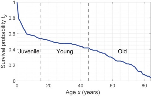
In keeping with Le et al.'s paper, we use life history data from the Hadza, a hunter-gatherer group living in northern Tanzania (Blurton Jones et al., 2002, Table 3). In their table, we are interested in the column showing the probabilities of surviving to age x, notated $l_x$, which we plot in Figure 2.

Figure 2. Survival curve from the Hadza lifetable of Blurton Jones et al. (2002, Table 3). We partition the population into three age classes: juvenile (age 0–15), young (age 15–45), and old (ages 45+).

Referring back to Section 2.1, we assume our populations are at stable age distributions. Furthermore, we assume $F_1$ and $F_2$ have the same age distribution, since they have the same mortality rates. To estimate the reproductive parameters a and b, we first estimate the proportions, ${\psi }_a$ and ${\psi }_b$, of younger and older females in the population. For simplicity, we assume the survival curve in Figure 2 approximates the stable age distribution, which is valid if the growth or decline rates of the total population is small.

In Figure 2, we plotted the survival probabilities $l_x$ for each year of age and joined them with lines. We then divided the data into Juveniles, Young, and Old. Juveniles are those between ages 0 to 15 who we assume have not reached sexual maturity, the Young are sexually mature females between ages 15 and 45, and the Old are females over 45. Using the survival curve, we can find the proportion of young females ${\psi }_a$ and old females ${\psi }_b$ by calculating the areas under various sections of the curve. This is a task that can be given to students.

For convenience of notation, let us assume $l(x)$ is a piecewise linear continuous function connecting the data points $l_x$ given by Blurton Jones et al. (2002). Also note that the data ends at age 84, so our integrals stop there rather than infinity. Using the trapezoidal rule to evaluate integrals, we estimate the proportion of younger and older females as follows: ${\psi }_a={\displaystyle \frac{{\int }_{15}^{45}l(x)\mathrm{d}x}{{\int }_0^{84}l(x)\mathrm{d}x}}=0.428\mathrm{and}{\psi }_b={\displaystyle \frac{{\int }_{45}^{84}l(x)\mathrm{d}a}{{\int }_0^{84}l(x)\mathrm{d}x}}=\mathrm{0.288.}$ Similarly, we estimate the average death rate, but this time, integrate across the entire age range: $\delta ={\displaystyle \frac{1}{{\int }_0^{84}l(x)\mathrm{d}x}}=0.030{\mathrm{yr}}^{-1}.$ In addition, we estimate the birth rate β using a chimpanzee average interbirth interval of 5 years (Thompson, 2013; Thompson et al., 2007). This results in a birth rate of $\beta =(1/2)\cdot (1/5){\mathrm{yr}}^{-1}=0.1{\mathrm{yr}}^{-1}$, where the factor of 1/2 is because we only account for female offspring and assume an equal probability of having children of either sex. Therefore, we estimate the reproductive contribution of young females to be $a={\psi }_a\beta =0.043{\mathrm{yr}}^{-1}$. For the reproductive contribution of old females in $F_1$, we have $b={\psi }_b\beta =0.029{\mathrm{yr}}^{-1}$. We set the mutation probability to be low at $\epsilon =0.0001$. These parameter estimates are summarised in Table 1.

2.3. Analysis using explicit solution

System (1(1) $\begin{array}{rl}\frac{\mathrm{d}{F}_1}{\mathrm{d}t}& =\underset{\begin{array}{c}\mathrm{Offspring}\mathrm{produced}\mathrm{by}\\ \mathrm{young}\mathrm{and}\mathrm{old}{F}_1\\ \mathrm{females}\mathrm{with}\mathrm{no}\mathrm{mutation}\end{array}}{\underbrace{(1-\epsilon )(a+\mathrm{\gamma b})F_1}}-\underset{\mathrm{Death}}{\underbrace{\delta F_1}},\end{array}$(1) ) and (2(2) $\begin{array}{rl}\frac{\mathrm{d}{F}_2}{\mathrm{d}t}& =\underset{\begin{array}{c}\mathrm{Offspring}\mathrm{produced}\mathrm{by}\\ \mathrm{young}\mathrm{and}\mathrm{old}{F}_1\\ \mathrm{females}\mathrm{with}\mathrm{mutation}\end{array}}{\underbrace{\epsilon (a+\mathrm{\gamma b})F_1}}+\underset{\begin{array}{c}\mathrm{Offspring}\mathrm{produced}\\ \mathrm{by}\mathrm{young}{F}_2\mathrm{females}\end{array}}{\underbrace{a{F}_2}}-\underset{\mathrm{Death}}{\underbrace{\delta F_2}},\end{array}$(2) ) can be written as (3) $\frac{\mathrm{d}}{\mathrm{d}t}\left(\begin{array}{c}{F}_1\\ F_2\end{array}\right)=\left(\begin{array}{cc}(1-\epsilon )(a+\mathrm{\gamma b})-\delta & 0\\ \epsilon (a+\mathrm{\gamma b})& a-\delta \end{array}\right)\left(\begin{array}{c}{F}_1\\ F_2\end{array}\right),$(3) and we can solve it explicitly. We can observe straightforwardly that the matrix has eigenvalues ${\lambda }_1=(1-\epsilon )(a+\mathrm{\gamma b})-\delta \mathrm{and}{\lambda }_2=a-\delta$ and determine the corresponding eigenvectors ${\mathbf{v}}_1=\left(\begin{array}{c}(1-\epsilon )\mathrm{\gamma b}-\mathrm{\epsilon a}\\ \epsilon (a+\mathrm{\gamma b})\end{array}\right)\mathrm{and}{\mathbf{v}}_2=\left(\begin{array}{c}0\\ 1\end{array}\right).$ Hence, the solution is $\left(\begin{array}{c}{F}_1\\ F_2\end{array}\right)=A{e}^{{\lambda }_{1}t}{\mathbf{v}}_1+B{e}^{{\lambda }_{2}t}{\mathbf{v}}_2$ for arbitrary constants A and B.

Exercise: Students can verify the eigenvalues and eigenvectors above. Alternatively, they could find the solution to (3(3) $\frac{\mathrm{d}}{\mathrm{d}t}\left(\begin{array}{c}{F}_1\\ F_2\end{array}\right)=\left(\begin{array}{cc}(1-\epsilon )(a+\mathrm{\gamma b})-\delta & 0\\ \epsilon (a+\mathrm{\gamma b})& a-\delta \end{array}\right)\left(\begin{array}{c}{F}_1\\ F_2\end{array}\right),$(3) ) on their own without being given the eigenvalues and eigenvectors.

There are two possible long-term outcomes. If ${\lambda }_1$ is the dominant eigenvalue, i.e. ${\lambda }_1>{\lambda }_2⟺\gamma >\frac{\epsilon }{1-\epsilon }\frac{a}{b},$ the proportion of females with lifelong fertility will approach $\frac{v_{11}}{v_{11}+v_{12}}=1-\epsilon (1+\frac{a}{\mathrm{\gamma b}}).$ If ${\lambda }_2$ is dominant, i.e. ${\lambda }_1<{\lambda }_2⟺\gamma <\frac{\epsilon }{1-\epsilon }\frac{a}{b},$ it will approach 0, meaning $F_2$ dominates.

Exercise: Students can verify the conclusions above.

2.4. Analysis by transforming the system to a 1-D ODE

As an alternative approach, note that we mainly care about whether lifelong fertility (trait 1) or old-age infertility (trait 2) dominates, so it suffices to look at the long-term proportions of $F_1$ and $F_2$ in the population rather than their actual values. Hence, let us define $U_1={\displaystyle \frac{F_1}{T}}\mathrm{and}{U}_2={\displaystyle \frac{F_2}{T}},$ where $T=F_1+F_2$ is the total population. These variables represent the proportions of traits 1 (lifelong fertility) and 2 (old-age infertility) in the population, so $U_1+U_2=1$.

Now, we derive an ODE for $U_1$.

We will need to calculate dT/dt, so adding (1(1) $\begin{array}{rl}\frac{\mathrm{d}{F}_1}{\mathrm{d}t}& =\underset{\begin{array}{c}\mathrm{Offspring}\mathrm{produced}\mathrm{by}\\ \mathrm{young}\mathrm{and}\mathrm{old}{F}_1\\ \mathrm{females}\mathrm{with}\mathrm{no}\mathrm{mutation}\end{array}}{\underbrace{(1-\epsilon )(a+\mathrm{\gamma b})F_1}}-\underset{\mathrm{Death}}{\underbrace{\delta F_1}},\end{array}$(1) ) and (2(2) $\begin{array}{rl}\frac{\mathrm{d}{F}_2}{\mathrm{d}t}& =\underset{\begin{array}{c}\mathrm{Offspring}\mathrm{produced}\mathrm{by}\\ \mathrm{young}\mathrm{and}\mathrm{old}{F}_1\\ \mathrm{females}\mathrm{with}\mathrm{mutation}\end{array}}{\underbrace{\epsilon (a+\mathrm{\gamma b})F_1}}+\underset{\begin{array}{c}\mathrm{Offspring}\mathrm{produced}\\ \mathrm{by}\mathrm{young}{F}_2\mathrm{females}\end{array}}{\underbrace{a{F}_2}}-\underset{\mathrm{Death}}{\underbrace{\delta F_2}},\end{array}$(2) ), we obtain $\begin{array}{rl}\frac{\mathrm{d}T}{\mathrm{d}t}& =\frac{\mathrm{d}{F}_1}{\mathrm{d}t}+\frac{\mathrm{d}{F}_2}{\mathrm{d}t}\\ & =(1-\epsilon )(a+\mathrm{\gamma b})F_1-\delta F_1+\epsilon (a+\mathrm{\gamma b})F_1+a{F}_2-\delta F_2\\ & =(a+\mathrm{\gamma b})F_1+a{F}_2-\mathrm{\delta T}.\end{array}$ Then, we take the derivative of both sides of $U_1=F_1/T$ using the product rule and (1(1) $\begin{array}{rl}\frac{\mathrm{d}{F}_1}{\mathrm{d}t}& =\underset{\begin{array}{c}\mathrm{Offspring}\mathrm{produced}\mathrm{by}\\ \mathrm{young}\mathrm{and}\mathrm{old}{F}_1\\ \mathrm{females}\mathrm{with}\mathrm{no}\mathrm{mutation}\end{array}}{\underbrace{(1-\epsilon )(a+\mathrm{\gamma b})F_1}}-\underset{\mathrm{Death}}{\underbrace{\delta F_1}},\end{array}$(1) ) and (2(2) $\begin{array}{rl}\frac{\mathrm{d}{F}_2}{\mathrm{d}t}& =\underset{\begin{array}{c}\mathrm{Offspring}\mathrm{produced}\mathrm{by}\\ \mathrm{young}\mathrm{and}\mathrm{old}{F}_1\\ \mathrm{females}\mathrm{with}\mathrm{mutation}\end{array}}{\underbrace{\epsilon (a+\mathrm{\gamma b})F_1}}+\underset{\begin{array}{c}\mathrm{Offspring}\mathrm{produced}\\ \mathrm{by}\mathrm{young}{F}_2\mathrm{females}\end{array}}{\underbrace{a{F}_2}}-\underset{\mathrm{Death}}{\underbrace{\delta F_2}},\end{array}$(2) ) to find $\begin{array}{rl}\frac{\mathrm{d}{U}_1}{\mathrm{d}t}& =\frac{1}{T}\frac{\mathrm{d}{F}_1}{\mathrm{d}t}-\frac{F_1}{T^2}\frac{\mathrm{d}T}{\mathrm{d}t}\\ & =\frac{(1-\epsilon )(a+\mathrm{\gamma b})F_1-\delta F_1}{T}-\frac{F_1}{T}\frac{(a+\mathrm{\gamma b})F_1+a{F}_2-\mathrm{\delta T}}{T}\\ & =(1-\epsilon )(a+\mathrm{\gamma b})U_1-\delta U_1-U_1((a+\mathrm{\gamma b})U_1+a{U}_2-\delta ).\end{array}$ Substituting $U_2=1-U_1$ and dropping the subscript 1 for convenience, we obtain (4) $\frac{\mathrm{d}U}{\mathrm{d}t}=((1-\epsilon )(a+\mathrm{\gamma b})-a-\mathrm{\gamma bU})U.$(4) Exercise: Derive (4(4) $\frac{\mathrm{d}U}{\mathrm{d}t}=((1-\epsilon )(a+\mathrm{\gamma b})-a-\mathrm{\gamma bU})U.$(4) ) from the definition of U and (1(1) $\begin{array}{rl}\frac{\mathrm{d}{F}_1}{\mathrm{d}t}& =\underset{\begin{array}{c}\mathrm{Offspring}\mathrm{produced}\mathrm{by}\\ \mathrm{young}\mathrm{and}\mathrm{old}{F}_1\\ \mathrm{females}\mathrm{with}\mathrm{no}\mathrm{mutation}\end{array}}{\underbrace{(1-\epsilon )(a+\mathrm{\gamma b})F_1}}-\underset{\mathrm{Death}}{\underbrace{\delta F_1}},\end{array}$(1) ) and (2(2) $\begin{array}{rl}\frac{\mathrm{d}{F}_2}{\mathrm{d}t}& =\underset{\begin{array}{c}\mathrm{Offspring}\mathrm{produced}\mathrm{by}\\ \mathrm{young}\mathrm{and}\mathrm{old}{F}_1\\ \mathrm{females}\mathrm{with}\mathrm{mutation}\end{array}}{\underbrace{\epsilon (a+\mathrm{\gamma b})F_1}}+\underset{\begin{array}{c}\mathrm{Offspring}\mathrm{produced}\\ \mathrm{by}\mathrm{young}{F}_2\mathrm{females}\end{array}}{\underbrace{a{F}_2}}-\underset{\mathrm{Death}}{\underbrace{\delta F_2}},\end{array}$(2) ).

Using (4(4) $\frac{\mathrm{d}U}{\mathrm{d}t}=((1-\epsilon )(a+\mathrm{\gamma b})-a-\mathrm{\gamma bU})U.$(4) ) we analyse the stability of this system by solving for equilibria. Letting $\mathrm{dU}/\mathrm{dt}=0$, we find $0=((1-\epsilon )(a+\mathrm{\gamma b})-a-\mathrm{\gamma bU})U,$ giving the two equilibrium points (5) $U=0\mathrm{and}U=\frac{(1-\epsilon )(a+\mathrm{\gamma b})-a}{\mathrm{\gamma b}}=1-\epsilon (1+\frac{a}{\mathrm{\gamma b}}).$(5) Note that the right-hand side of (4(4) $\frac{\mathrm{d}U}{\mathrm{d}t}=((1-\epsilon )(a+\mathrm{\gamma b})-a-\mathrm{\gamma bU})U.$(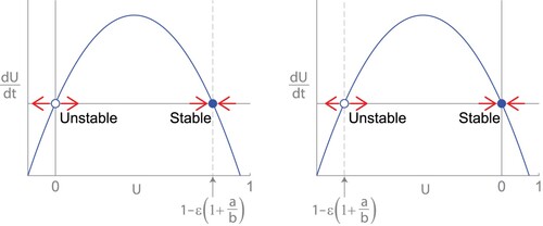4) ) is a downward parabola, so when the second equilibrium is positive, it is stable and U=0 is unstable (see Figure 3(a)). On the other hand, if the second equilibrium is negative, it is unstable and U=0 is stable (see Figure 3(b)).

Figure 3. Growth curves dU/dt vs U for (4(4) $\frac{\mathrm{d}U}{\mathrm{d}t}=((1-\epsilon )(a+\mathrm{\gamma b})-a-\mathrm{\gamma bU})U.$(4) ). (a) When $0<1-\epsilon (1+a/b)$, the positive equilibrium is stable and U=0 is unstable. (b) When $0<1-\epsilon (1+a/b)$, the equilibrium at U=0 is stable and the negative equilibirum is unstable.

Exercise: Conduct or verify the stability analysis above.

Exercise: Draw the bifurcation diagram for (4(4) $\frac{\mathrm{d}U}{\mathrm{d}t}=((1-\epsilon )(a+\mathrm{\gamma b})-a-\mathrm{\gamma bU})U.$(4) ) with respect to bifurcation parameter γ. What kind of bifurcation is it?

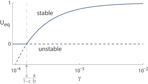
To draw the bifurcation diagram, we plot the two equilibrium points given in (5(5) $U=0\mathrm{and}U=\frac{(1-\epsilon )(a+\mathrm{\gamma b})-a}{\mathrm{\gamma b}}=1-\epsilon (1+\frac{a}{\mathrm{\gamma b}}).$(5) ). We calculate that they intersect at the bifurcation point $\gamma =\frac{\epsilon }{1-\epsilon }\frac{a}{b}.$ Furthermore, from our stability analysis above, we know that the two equilibria change stability at this point, and the equilibrium with the greater value is stable. This is a transcritical bifurcation, and we can draw the bifurcation diagram in Figure 4.

Figure 4. Bifurcation diagram of equilibrium points $U_{\mathrm{eq}}$ for the proportion of females with trait 1 (lifelong fertility) for various values of γ, the probability old, fertile females find mates. Equilibria cross at a transcritical bifurcation at $\gamma =(\epsilon /(1-\epsilon ))(a/b)$, where they swap stabilities.

Substituting the parameter estimates from Table 1, we find that γ, the probability an old, fertile female finds a mate, has to be extremely small for old-age infertility (trait 2) to dominate. In fact, we can find the point where the stable equilibrium value of U is 0.5, the balance point, by solving $U_{\mathrm{eq}}=1-\epsilon (1+\frac{a}{\mathrm{\gamma b}})=0.5⟹\gamma =\frac{\epsilon }{0.5-\epsilon }\frac{a}{b}=3.0\times {10}^{-4}.$ Thus, unless γ is very small (i.e. $\gamma \le 0.0003$), the proportion of females with lifelong fertility (trait 1) makes up the majority of the population at the stable equilibrium. In fact, for $\gamma =0.05\mathrm{\%}$, $0.1\mathrm{\%}$, and $1\mathrm{\%}$, the fractions of females with lifelong fertility (trait 1) in the long term are 0.70, 0.85, and 0.99 repsectively. Evidently, this means that even if the chances of older females finding a mate is low, that small proportion of older females who reproduce at older ages is enough to maintain old-age female fertility as the dominant trait. We can infer that for a shift to old-age infertility to occur, the males must severely limit their mate choice. However, in this section, we have not considered the male population explicitly. Therefore, in the following section, we add two male populations. This allows us to investigate Morton et al.'s conclusion further.

3. Two-sex model with mutating end of female fertility and varying male mating preference

3.1. Model

In Section 2, we started with a simple a female-only model by assuming a fixed probability γ that an old female will find a mate. We next introduce some variability in male mating preferences by introducing two male populations:

1. Unfussy males ($M_1$) who are willing to mate with a female of any age,

2. Fussy males ($M_2$) who only mate young females.

For simplicity, we assume every time a female is ready to mate, she has one chance to pair up and chooses among all available mates with equal chance. In this case, the probability γ that an old female successfully reproduces is the chance of randomly picking an unfussy male, so (6) $\gamma =\frac{M_1}{T_M},$(6) where $T_M=M_1+M_2$ is the total male population. As before, we assume young females always successfully mate. Then, substituting (6(6) $\gamma =\frac{M_1}{T_M},$(6) ) into our previous model (1(1) $\begin{array}{rl}\frac{\mathrm{d}{F}_1}{\mathrm{d}t}& =\underset{\begin{array}{c}\mathrm{Offspring}\mathrm{produced}\mathrm{by}\\ \mathrm{young}\mathrm{and}\mathrm{old}{F}_1\\ \mathrm{females}\mathrm{with}\mathrm{no}\mathrm{mutation}\end{array}}{\underbrace{(1-\epsilon )(a+\mathrm{\gamma b})F_1}}-\underset{\mathrm{Death}}{\underbrace{\delta F_1}},\end{array}$(1) ) and (2(2) $\begin{array}{rl}\frac{\mathrm{d}{F}_2}{\mathrm{d}t}& =\underset{\begin{array}{c}\mathrm{Offspring}\mathrm{produced}\mathrm{by}\\ \mathrm{young}\mathrm{and}\mathrm{old}{F}_1\\ \mathrm{females}\mathrm{with}\mathrm{mutation}\end{array}}{\underbrace{\epsilon (a+\mathrm{\gamma b})F_1}}+\underset{\begin{array}{c}\mathrm{Offspring}\mathrm{produced}\\ \mathrm{by}\mathrm{young}{F}_2\mathrm{females}\end{array}}{\underbrace{a{F}_2}}-\underset{\mathrm{Death}}{\underbrace{\delta F_2}},\end{array}$(2) ), we obtain the ODEs (7) $\begin{array}{rl}\frac{\mathrm{d}{F}_1}{\mathrm{d}t}& =(1-\epsilon )(a+b\cdot \frac{M_1}{T_M})F_1-\delta F_1,\end{array}$(7) (8) $\begin{array}{rl}\frac{\mathrm{d}{F}_2}{\mathrm{d}t}& =\epsilon (a+b\cdot \frac{M_1}{T_M})F_1+a{F}_2-\delta F_2,\end{array}$(8) for the female populations. For the males, we write the model (9) $\begin{array}{rl}\frac{\mathrm{d}{M}_1}{\mathrm{d}t}& =\underset{\begin{array}{c}\mathrm{Mating}\mathrm{rate}\mathrm{of}{M}_1\mathrm{with}\\ \mathrm{young}\mathrm{and}\mathrm{old}\mathrm{females}\end{array}}{\underbrace{((a+b)F_1+a{F}_2)\frac{M_1}{T_M}}}-\underset{\mathrm{Death}}{\underbrace{\delta M_1}},\end{array}$(9) (10) $\begin{array}{rl}\frac{\mathrm{d}{M}_2}{\mathrm{d}t}& =\underset{\begin{array}{c}\mathrm{Mating}\mathrm{rate}\mathrm{of}{M}_2\mathrm{with}\\ \mathrm{young}\mathrm{females}\end{array}}{\underbrace{(a{F}_1+a{F}_2)\frac{M_2}{T_M}}}-\underset{\mathrm{Death}}{\underbrace{\delta M_2}}.\end{array}$(10) The mating rates for the male equations above are constructed as follows. The total number of fertile females is $(a+b)F_1+a{F}_2$, which includes young and old females from $F_1$ and young females from $F_2$. The probability these females mate with an unfussy male is $M_1/T_M$, so the mating rate of $M_1$ males with fertile females is given by the first term in (9(9) $\begin{array}{rl}\frac{\mathrm{d}{M}_1}{\mathrm{d}t}& =\underset{\begin{array}{c}\mathrm{Mating}\mathrm{rate}\mathrm{of}{M}_1\mathrm{with}\\ \mathrm{young}\mathrm{and}\mathrm{old}\mathrm{females}\end{array}}{\underbrace{((a+b)F_1+a{F}_2)\frac{M_1}{T_M}}}-\underset{\mathrm{Death}}{\underbrace{\delta M_1}},\end{array}$(9) ). Similarly, the total number of young females is $a{F}_1+a{F}_2$, and the probability they mate with a fussy male is $M_2/T_M$, so the mating rate of $M_2$ males with young females is given by the first term in (10(10) $\begin{array}{rl}\frac{\mathrm{d}{M}_2}{\mathrm{d}t}& =\underset{\begin{array}{c}\mathrm{Mating}\mathrm{rate}\mathrm{of}{M}_2\mathrm{with}\\ \mathrm{young}\mathrm{females}\end{array}}{\underbrace{(a{F}_1+a{F}_2)\frac{M_2}{T_M}}}-\underset{\mathrm{Death}}{\underbrace{\delta M_2}}.\end{array}$(10) ). Note that we assume an equal chance of having sons and daughters, so the reproductive rates a and b also give the rates females produce sons, which is why we can use them directly in the equations for males. As with the females, we also assume males die at rate δ, giving the last terms of (9(9) $\begin{array}{rl}\frac{\mathrm{d}{M}_1}{\mathrm{d}t}& =\underset{\begin{array}{c}\mathrm{Mating}\mathrm{rate}\mathrm{of}{M}_1\mathrm{with}\\ \mathrm{young}\mathrm{and}\mathrm{old}\mathrm{females}\end{array}}{\underbrace{((a+b)F_1+a{F}_2)\frac{M_1}{T_M}}}-\underset{\mathrm{Death}}{\underbrace{\delta M_1}},\end{array}$(9) ) and (10(10) $\begin{array}{rl}\frac{\mathrm{d}{M}_2}{\mathrm{d}t}& =\underset{\begin{array}{c}\mathrm{Mating}\mathrm{rate}\mathrm{of}{M}_2\mathrm{with}\\ \mathrm{young}\mathrm{females}\end{array}}{\underbrace{(a{F}_1+a{F}_2)\frac{M_2}{T_M}}}-\underset{\mathrm{Death}}{\underbrace{\delta M_2}}.\end{array}$(10) ).

We have not included mutation between $M_1$ and $M_2$, because adding it makes the analysis more algebraically intense. However, one could analyse a system with mutations in the same way we analyse this system in Section 3.2.

Thought question: What if we assume fertile females have more than one chance to find a mate or if they have some agency of choice rather than selecting randomly? How would that change the expression for γ in (6(6) $\gamma =\frac{M_1}{T_M},$(6) )?

3.2. Analysis

Model (7(7) $\begin{array}{rl}\frac{\mathrm{d}{F}_1}{\mathrm{d}t}& =(1-\epsilon )(a+b\cdot \frac{M_1}{T_M})F_1-\delta F_1,\end{array}$(7) )–(10(10) $\begin{array}{rl}\frac{\mathrm{d}{M}_2}{\mathrm{d}t}& =\underset{\begin{array}{c}\mathrm{Mating}\mathrm{rate}\mathrm{of}{M}_2\mathrm{with}\\ \mathrm{young}\mathrm{females}\end{array}}{\underbrace{(a{F}_1+a{F}_2)\frac{M_2}{T_M}}}-\underset{\mathrm{Death}}{\underbrace{\delta M_2}}.\end{array}$(10) ) is a 4-D nonlinear ODE system making it difficult to analyse without simplifying. First, let $T_F=F_1+F_2$ and $T_M=M_1+M_2$ be the total female and male populations respectively. Adding (7(7) $\begin{array}{rl}\frac{\mathrm{d}{F}_1}{\mathrm{d}t}& =(1-\epsilon )(a+b\cdot \frac{M_1}{T_M})F_1-\delta F_1,\end{array}$(7) ) and (8(8) $\begin{array}{rl}\frac{\mathrm{d}{F}_2}{\mathrm{d}t}& =\epsilon (a+b\cdot \frac{M_1}{T_M})F_1+a{F}_2-\delta F_2,\end{array}$(8) ), we get $\frac{\mathrm{d}{T}_F}{\mathrm{d}t}=\frac{\mathrm{d}{F}_1}{\mathrm{d}t}+\frac{\mathrm{d}{F}_2}{\mathrm{d}t}=\underset{f(t)}{\underbrace{(a+b\cdot \frac{M_1}{T_M})F_1+a{F}_2}}-\delta T_F,$ and adding (9(9) $\begin{array}{rl}\frac{\mathrm{d}{M}_1}{\mathrm{d}t}& =\underset{\begin{array}{c}\mathrm{Mating}\mathrm{rate}\mathrm{of}{M}_1\mathrm{with}\\ \mathrm{young}\mathrm{and}\mathrm{old}\mathrm{females}\end{array}}{\underbrace{((a+b)F_1+a{F}_2)\frac{M_1}{T_M}}}-\underset{\mathrm{Death}}{\underbrace{\delta M_1}},\end{array}$(9) ) and (10(10) $\begin{array}{rl}\frac{\mathrm{d}{M}_2}{\mathrm{d}t}& =\underset{\begin{array}{c}\mathrm{Mating}\mathrm{rate}\mathrm{of}{M}_2\mathrm{with}\\ \mathrm{young}\mathrm{females}\end{array}}{\underbrace{(a{F}_1+a{F}_2)\frac{M_2}{T_M}}}-\underset{\mathrm{Death}}{\underbrace{\delta M_2}}.\end{array}$(10) ), we get $\frac{\mathrm{d}{T}_M}{\mathrm{d}t}=\frac{\mathrm{d}{M}_1}{\mathrm{d}t}+\frac{\mathrm{d}{M}_2}{\mathrm{d}t}=\underset{f(t)}{\underbrace{(a+b\cdot \frac{M_1}{T_M})F_1+a{F}_2}}-\delta T_M.$ Note that $T_F$ and $T_M$ satisfy the same differential equation $(\frac{\mathrm{d}}{\mathrm{d}t}+\delta )T_F=f(t)\mathrm{and}(\frac{\mathrm{d}}{\mathrm{d}t}+\delta )T_M=f(t),$ where $f(t)=(a+b\cdot \frac{M_1}{T_M})F_1+a{F}_2.$ By uniqueness of solutions to ODEs, as long as the initial conditions $T_F(0)=T_M(0)$ match, we have $T_F(t)=T_M(t)$ for all t. Hence, let us assume the total female and male populations start at the same value and define $T=T_F=T_M$ as the total populations of males or females.

Similarly to what we did before, define the normalised populations $\begin{array}{rl}& U_1=\frac{F_1}{T},U_2=\frac{F_2}{T},\\ & V_1=\frac{M_1}{T},V_2=\frac{M_2}{T}.\end{array}$ Note that $U_1+U_2=1$ and $V_1+V_2=1$, so let us define $U=U_1$ and $1-U=U_2$; and $V=V_1$ and $1-V=V_2$.

Now, we will take the system (7(7) $\begin{array}{rl}\frac{\mathrm{d}{F}_1}{\mathrm{d}t}& =(1-\epsilon )(a+b\cdot \frac{M_1}{T_M})F_1-\delta F_1,\end{array}$(7) )–(10(10) $\begin{array}{rl}\frac{\mathrm{d}{M}_2}{\mathrm{d}t}& =\underset{\begin{array}{c}\mathrm{Mating}\mathrm{rate}\mathrm{of}{M}_2\mathrm{with}\\ \mathrm{young}\mathrm{females}\end{array}}{\underbrace{(a{F}_1+a{F}_2)\frac{M_2}{T_M}}}-\underset{\mathrm{Death}}{\underbrace{\delta M_2}}.\end{array}$(10) ) and derive an ODE system for U and V . As before, we differentiate $U_1$ using the product rule and chain rule to obtain $\frac{\mathrm{d}{U}_1}{\mathrm{d}t}=\frac{1}{T}\frac{\mathrm{d}{F}_1}{\mathrm{d}t}-\frac{F_1}{T^2}\frac{\mathrm{d}T}{\mathrm{d}t},$ so $\begin{array}{rl}\frac{\mathrm{d}{U}_1}{\mathrm{d}t}& =\frac{1}{T}((1-\epsilon )(a+b\cdot \frac{M_1}{T})F_1-\delta F_1)-\frac{F_1}{T^2}((a+b\cdot \frac{M_1}{T})F_1+a{F}_2-\mathrm{\delta T})\\ & =(1-\epsilon )(a+b{V}_1)U_1-\delta U_1-U_1((a+b{V}_1)U_1+a{U}_2-\delta ).\end{array}$ Substituting $U_1=U$, $U_2=1-U$, and $V_1=V$, we obtain $\begin{array}{rl}\frac{\mathrm{d}U}{\mathrm{d}t}& =(1-\epsilon )(a+\mathrm{bV})U-\mathrm{\delta U}-U((a+\mathrm{bV})U+a(1-U)-\delta )\\ & =(b(1-\epsilon -U)V-\mathrm{\epsilon a})U.\end{array}$ Exercise: Verify the derivation above. Alternatively, one could ask students to produce the ODE for U without seeing the steps.

Similarly, for V , one will obtain the ODE $\frac{\mathrm{d}V}{\mathrm{d}t}=\mathrm{bUV}(1-V),$ and as a check, we can verify that $\begin{array}{r}\frac{\mathrm{d}{U}_2}{\mathrm{d}t}=-\frac{\mathrm{d}U}{\mathrm{d}t}\mathrm{and}\frac{\mathrm{d}{V}_2}{\mathrm{d}t}=-\frac{\mathrm{d}V}{\mathrm{d}t}.\end{array}$ Exercise: Verify the results above.

Hence, we have reduced the original 4-D system (7(7) $\begin{array}{rl}\frac{\mathrm{d}{F}_1}{\mathrm{d}t}& =(1-\epsilon )(a+b\cdot \frac{M_1}{T_M})F_1-\delta F_1,\end{array}$(7) )–(10(10) $\begin{array}{rl}\frac{\mathrm{d}{M}_2}{\mathrm{d}t}& =\underset{\begin{array}{c}\mathrm{Mating}\mathrm{rate}\mathrm{of}{M}_2\mathrm{with}\\ \mathrm{young}\mathrm{females}\end{array}}{\underbrace{(a{F}_1+a{F}_2)\frac{M_2}{T_M}}}-\underset{\mathrm{Death}}{\underbrace{\delta M_2}}.\end{array}$(10) ) to the 2-D system (11) $\begin{array}{rl}\frac{\mathrm{d}U}{\mathrm{d}t}& =(b(1-\epsilon -U)V-\mathrm{\epsilon a})U,\end{array}$(11) (12) $\begin{array}{rl}\frac{\mathrm{d}V}{\mathrm{d}t}& =\mathrm{bUV}(1-V).\end{array}$(12) Exercise: Analyse the system (11(11) $\begin{array}{rl}\frac{\mathrm{d}U}{\mathrm{d}t}& =(b(1-\epsilon -U)V-\mathrm{\epsilon a})U,\end{array}$(11) ) and (12(12) $\begin{array}{rl}\frac{\mathrm{d}V}{\mathrm{d}t}& =\mathrm{bUV}(1-V).\end{array}$(12) ) by finding nullclines, equilibria, and characterising equilibria. Draw the phase portrait.

In a nonlinear ODEs course, students ought to be able to carry out the analysis above with the catch that the system above has a line of (unstable) equilibrium points at $U=0$, which they might find unexpected. We do the analysis below for reference.

The U-nullclines are $U=0\mathrm{and}V=\frac{\mathrm{\epsilon a}}{b(1-\epsilon -U)},$ and the V -nullclines are $U=0,V=0,\mathrm{and}V=1.$ We plot the nullclines in Figure 5.

Figure 5. Phase plane for (11(11) $\begin{array}{rl}\frac{\mathrm{d}U}{\mathrm{d}t}& =(b(1-\epsilon -U)V-\mathrm{\epsilon a})U,\end{array}$(11) ) and (12(12) $\begin{array}{rl}\frac{\mathrm{d}V}{\mathrm{d}t}& =\mathrm{bUV}(1-V).\end{array}$(12) ). The population U is the proportion of females with lifelong fertility as opposed to old-age infertility, and V is the proportion of males who are unfussy and will mate with females of any age as opposed to fussy males who only mate young females. (Note that the figure is not drawn to scale to make certain features more prominent. In fact, it is generated by setting an artificially high mutation rate $\epsilon =0.05$ and taking other parameter values from Table 1.)

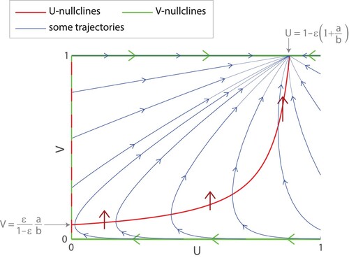
We can find that the U-nullcline given by $V=\frac{\mathrm{\epsilon a}}{b(1-\epsilon -U)}$ intersects the V -nullclines U=0 and V =1 at $(0,\frac{\epsilon }{1-\epsilon }\frac{a}{b})\mathrm{and}(1-\epsilon (1+\frac{a}{b}),1)$ respectively. By considering the directions of the vector field along the nullclines, we can observe the following:

• The fixed points are the line U=0 and the point $(1-\epsilon (1+a/b),1)$.

• The fixed point $(1-\epsilon (1+a/b),1)$ is a stable node.

• If we use the definition of stable and unstable slightly loosely, the points along the line U=0 with $V>\frac{\epsilon }{1-\epsilon }\frac{a}{b}$ are unstable (i.e. one eigenvalue is positive and the other is 0) and the points with $V<\frac{\epsilon }{1-\epsilon }\frac{a}{b}$ are stable (i.e. one eigenvalue is negative and the other is 0).

Exercise: Alternatively, students can verify the bulleted results above by calculating the Jacobian of (11(11) $\begin{array}{rl}\frac{\mathrm{d}U}{\mathrm{d}t}& =(b(1-\epsilon -U)V-\mathrm{\epsilon a})U,\end{array}$(11) ) and (12(12) $\begin{array}{rl}\frac{\mathrm{d}V}{\mathrm{d}t}& =\mathrm{bUV}(1-V).\end{array}$(12) ) and evaluating it at the various equilibrium points.

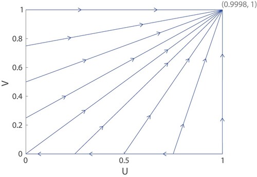
Note that the phase plane in Figure 5 is not drawn to scale. The mutation probability ε is artificially raised to 0.05 to make certain features of the phase plane more prominent. If we draw the phase plane with all parameters as in Table 1, including $\epsilon =0.0001$, we obtain the trajectories in Figure 6. Here, nearly all the trajectories look like straight lines heading directly towards the stable node at $(1-\epsilon (1+\frac{a}{b}),1)=(0.9998,1).$

Figure 6. Trajectories for (11(11) $\begin{array}{rl}\frac{\mathrm{d}U}{\mathrm{d}t}& =(b(1-\epsilon -U)V-\mathrm{\epsilon a})U,\end{array}$(11) ) and (12(12) $\begin{array}{rl}\frac{\mathrm{d}V}{\mathrm{d}t}& =\mathrm{bUV}(1-V).\end{array}$(12) ) using parameters from Table 1, including $\epsilon =0.0001$. Nearly all trajectories approach the stable node at $(U,V)=(0.9998,1)$. The population U is the proportion of females with lifelong fertility as opposed to old-age infertility, and V is the proportion of males who are unfussy and will mate with females of any age as opposed to fussy males who only mate young females.

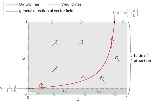
Note that for any initial population satisfying $U(0)>0\mathrm{and}V>\frac{\epsilon }{1-\epsilon }\frac{a}{b},$ the trajectory always has a positive $\mathrm{d}V/\mathrm{d}t$ and is repelled from the line of equilibria at U=0, so it is guaranteed to approach the stable node $(1-\epsilon (1+a/b),1)$ at the upper right corner. In fact, from numerical simulations, the basin of attraction for this stable node appears even larger, but precisely determining the bottom boundary is difficult. (See Figure 7, which is drawn to the scale of Figure 5 to make features more visible.)

Nonetheless, this observation implies that if the population contains at least a tiny minority of less choosy, unfussy males, specifically if $V(0)>\frac{\epsilon }{1-\epsilon }\frac{a}{b}=1.5\times {10}^{-4}$ (when using parameters from Table 1), the unfussy population will quickly outcompete and replace the fussy one. In addition, $U=\epsilon (1+a/b)=99.98\mathrm{\%}$ of the female population will maintain lifelong fertility. Therefore, our analysis in Sections 2 and 3 strongly imply that a male mating strategy of only mating young females is highly evolutionarily unstable. Furthermore, unless the vast majority of men never deviate from the preference to only mate young women, the most likely outcome of the male mate choice hypothesis is that we end up with a species in which fertile women of any age can find mates and the vast majority of women maintain lifelong fertility. Since this outcome is not true for our species, it seems we need an alternative hypothesis to explain human postmenopausal longevity. This is a task for future investigation.

Figure 7. Basin of attraction for the stable node $(1-\epsilon (1+a/b),1)$. We can observe that all trajectories starting in the light grey region with U>0 and $V>(\epsilon /(1-\epsilon ))(a/b)$ have positive dV/dt and are repelled from the line of equilibria at U=0, so they are guaranteed to approach the stable node $(1-\epsilon (1+a/b),1)$. From numerical simulations, we find that the basin of attraction includes an additional region in dark grey below the dashed line $V=(\epsilon /(1-\epsilon ))(a/b)$. (Note that this figure is not drawn to the correct scale as in Figure 6. It is drawn to the scale of Figure 5.).

4. Discussion

We have presented two systems of ODEs modelling the evolution of human postmenopausal longevity. We show how to analyse these systems using concepts taught in most second or third-year courses on nonlinear ODEs. The student exercises we propose include explicitly solving a linear 2-D ODE system, drawing a bifurcation diagram of a nonlinear ODE, and drawing a phase plane of a nonlinear 2-D ODE system.

To summarise the premise that inspired these models, Morton et al. proposed a male mate-choice hypothesis to explain the evolution of human postmenopausal longevity and constructed an ABM to justify it (Morton et al., 2013). Then, Le et al. (2022) pointed out that due to the complex nature of ABMs, certain features of their model may have remained unexplored and developed an ODE system of the hypothesis. Based on the model in Le et al. (2022), we construct two relatively simple ODE models presented in this article to investigate Morton et al.'s conclusions.

Both models presented in Sections 2 and 3 agree with Morton et al. that strict male mating preferences towards young females can lead to old-age infertility, or menopause, evolving. However, this occurs only under the most stringent condition that the vast majority of males collectively decide not to mate with any older females. From Figure 4 in Section 2, we can see that if a small number of males choose to mate with older females, it is enough to maintain lifelong female fertility. This is further supported in Section 3 where we added more variation by explicitly modelling males and their preferences traits. We see in Figure 6 that for almost any initial population of unfussy males, they will eventually outcompete fussy males. This is because fussy males who restrict their mate choice to only young females limit the chance of passing their fussy traits to the next generation whereas unfussy males, who will mate with females of any age, produce more offspring. For this reason, Morton et al.'s conclusions are too sensitive, relying on the specific condition that ancestral males collectively limit their mate choices to only young females. Hence, an alternative explanation to human postmenopausal longevity that does not hinge on the restriction of mate choice is needed.

We turn to current anthropological literature where the most widely supported theory is the Grandmother hypothesis. This theory centres around the economic productivity of older, less fertile, ancestral women subsiding care for kin. By doing so, these philanthropic older females facilitate the evolution of favourable traits such as extended lifespans and old-age infertility, which give rise to human postmenopausal longevity, without the need for any restrictions on mate choice (Hawkes, 2020; Hawkes & Coxworth, 2013; Hawkes et al., 1989, 2000, 1998; O'Connell et al., 1999b). Formulating and investigating an ODE model of the Grandmother hypothesis remains a challenge we aspire to address.

Acknowledgments

The authors would like to thank Emeritus Prof Mark Gould for guidance on analytical stability analysis and how to best evoke interest in students in this area from his years of lecturing, A/Prof Mark Nelson for examples and guidance on how to organise the article, and Dr Matthew Cody Nitschke for discussions during our planning phase.

Disclosure statement

No potential conflict of interest was reported by the authors.

Additional information

Funding

PSK was supported by the Australian Research Council Future Fellowship (FT200100190).

References

- Blurton Jones, N. G., Hawkes, K., & O'Connell, J. F. (2002). Antiquity of postreproductive life: Are there modern impacts on hunter-gatherer postreproductive life spans? American Journal of Human Biology, 14(2), 184–205. https://doi.org/10.1002/ajhb.v14:2
- Hawkes, K. (2020, September). The centrality of ancestral grandmothering in human evolution. Integrative and Comparative Biology, 60(3), 765–781. https://doi.org/10.1093/icb/icaa029
- Hawkes, K., & Coxworth, J. E. (2013). Grandmothers and the evolution of human longevity: A review of findings and future directions. Evolutionary Anthropology: Issues, News, and Reviews, 22(6), 294–302. https://doi.org/10.1002/evan.v22.6
- Hawkes, K., O'Connell, J. F., & Blurton Jones, N. G. (1989). Hardworking Hadza grandmothers. In V. Standen R. A. Foley (Eds.), Comparative socioecology: the behavioural ecology of humans and other mammals (pp. 341–366). Basil Blackwell.
- Hawkes, K., O'Connell, J. F., Blurton Jones, N. G., Alvarez, H., & Charnov, E. L. (2000). The grandmother hypothesis and human evolution. In Adaptation and human behavior: An anthropological perspective (Vol. 231, p. 252). Routledge.
- Hawkes, K., O'Connell, J. F., Jones, N. G., Alvarez, H., & Charnov, E. L. (1998, February). Grandmothering, menopause, and the evolution of human life histories. Proceedings of the National Academy of Sciences USA, 95(3), 1336–1339. https://doi.org/10.1073/pnas.95.3.1336
- Kaplan, H., Hill, K., Lancaster, J., & Hurtado, A. M. (2000). A theory of human life history evolution: Diet, intelligence, and longevity. Evolutionary Anthropology: Issues, News, and Reviews: Issues, News, and Reviews, 9(4), 156–185. https://doi.org/10.1002/(ISSN)1520-6505
- Le, A., Hawkes, K., & Kim, P. S. (2022, June). Male mating choices: The drive behind menopause? Theoretical Population Biology, 145, 126–135. https://doi.org/10.1016/j.tpb.2022.04.001
- Morton, R. A., Stone, J. R., & Singh, R. S. (2013). Mate choice and the origin of menopause. PLOS Computational Biology, 9(6), e1003092. https://doi.org/10.1371/journal.pcbi.1003092
- O'Connell, J. F., Hawkes, K., & Blurton Jones, N. G. (1999a, May). Grandmothering and the evolution of homo erectus. Journal of Human Evolution, 36(5), 461–485. https://doi.org/10.1006/jhev.1998.0285
- O'Connell, J. F., Hawkes, K., & Blurton Jones, N. G. (1999b, May). Grandmothering and the evolution of homo erectus. Journal of Human Evolution, 36(5), 461–485. https://doi.org/10.1006/jhev.1998.0285
- Parkinson, C. (2013, June). Men ‘to blame for the menopause’. BBC News website https://www.bbc.com/news/health-22886668.
- Saini, A. (2017). Inferior: How science got women wrong and the new research that's rewriting the story / angela saini. Beacon Press.
- Thompson, M. E. (2013, March). Reproductive ecology of female chimpanzees. American Journal of Primatology, 75(3), 222–237. https://doi.org/10.1002/ajp.2013.75.issue-3
- Thompson, M. E., Jones, J. H., Pusey, A. E., Brewer-Marsden, S., Goodall, J., Marsden, D., & Wrangham, R. W. (2007, December). Aging and fertility patterns in wild chimpanzees provide insights into the evolution of menopause. Current Biology, 17(24), 2150–2156. https://doi.org/10.1016/j.cub.2007.11.033
- Wrangham, R. W. (2001). Out of the pan, into the fire: How our ancestors' evolution depended on what they ate. In Tree of origin: What primate behavior can tell us about human social evolution (pp. 121–43). Harvard University Press.