Application of the method of lines to the wave equation for simulating vibrating strings

Abstract

This paper presents simulations of continuous dynamic models of vibrating strings for several different instruments: a guitar, a piano and a violin. The basis for all three models is the wave equation and is differentiated by the initial and boundary conditions imposed. The models are implemented as part of a Graphical User Interface. The simulations are presented as animations that are conveyed in the paper as a sequence of vibrating string profiles for different times. This paper promotes the idea that using music generation as a framework for teaching dynamics makes the teaching of dynamics a more engaging process.

A case is made that there is value in solving the wave equation numerically using the method of lines rather than looking for analytical solutions. The reason for this is the mathematics of the method of lines is simpler to understand than the techniques used to derive analytical solutions to partial differential equations. The numerical approach is also more easily extended to a more sophisticated model for a vibrating string that might include energy dissipation and the stiffness properties of the string.

KEYWORDS:

• Wave equation
• method of lines
• GUI
• animation
• music generation

Nomenclature

A	=	Matrix used to define a second-order ODE system (–)
ak	=	Coefficient in the analytical solution to the wave equation (–)
c	=	Wave speed (m/s)
CD	=	Constant in the energy dissipation term (–)
dx	=	An infinitesimal length of a string (m)
E	=	Youngs modulus (N/m2)
Ff	=	Friction force (N)
Ff,max	=	Maximum friction force (N)
fi	=	Natural frequency (Hz)
I	=	Second moment of area (m4)
IN	=	Identity matrix of order NxN (–)
L	=	Length of a string (m)
N	=	Number of lines in the method of lines (–)
Nbow	=	Reaction force of the bow (N)
Nk	=	Number of terms in the analytical solution of the wave equation (–)
T	=	Tension in a string (N)
tst	=	The time the stick stage starts in a violin simulation (s)
Vbow	=	Bow speed (m/s)
x	=	Independent variable of the wave equation (m)
xi	=	The location of line i in the method of lines (m)
Y	=	Vector of dependent variables in a 1st order ODE system (–)
y	=	Displacement of a vibrating string (m)
yi	=	Displacement for line i in the method of lines (m)
ymax	=	Maximum distortion of a string (m)
yst	=	Displacement of a violin string at L/2 at the start of the stick stage (m)

Greek letters

Δt	=	Time interval between vibrating string profiles (s)
Δx	=	Space-step (m)
Δxb	=	Base of an initial pulse in a piano string (m)
λi	=	Eigenvalues of the matrix A (–)
μS	=	Static coefficient of friction (–)
θ	=	Angle the vibrating string makes with the x axis (rad)
θ*	=	Angle the vibrating string makes with the x axis when approximating the violin string to be piecewise linear (rad)
ρ	=	Mass per unit length (g/m)
ωi	=	Natural frequency (rad/s)

1. Introduction

Machine dynamics is a mechanical engineering science that is steeped in mathematics. Historically many engineering students find machine dynamics a difficult topic to grasp. Over the last few decades, a weakness in the mathematical skills of many engineering students is a recognised issue. Many investigators have attempted to quantify and provide solution strategies to address the weakness in mathematics (Berry et al., 1989; Biggoggero and Rovida, 1977; Graham and Peek, 1997; Graham and Rowlands, 2000). One issue with mathematics and dynamics is that some students find it difficult to see the relevance of their early courses to the real world.

This paper addresses this issue by highlighting some connections between dynamics and something many young engineers have an interest in, music. This is done by the modelling of stringed instruments using continuous dynamic models. This is an advanced area of dynamics usually considered in an advanced course in dynamics. In this paper, a strategy for presentation and solution of continuous models is given that will allow an engineering student in dynamics to cut through the mathematics to appreciate the way continuous systems can be modelled. The focus in this paper is to illustrate the dynamics rather than get lost in the mathematical rigour of deriving analytical solutions to partial differential equations. Making connections between introductory, intermediate and advanced courses in dynamics is important. It goes some way to explaining to an engineering student that investment in dynamics as an engineering science is worthwhile, rather than something that must be survived until it is dropped at the first opportunity. One of the messages of this paper is that dynamics is something to be appreciated.

A further consideration is this paper addresses the solution of partial differential equations, not by looking for analytical solutions that may require a deep mathematical insight or use of mathematical ‘tricks’, to one based on a semi-discretisation of the continuous model using the method of lines (Campo, 2022; Reddy and Trefethen, 1992; Schiesser, 1993).

2. Literature review

There have been many investigations into the problem of poor mathematical skills of engineering students. In University of Cambridge NRICH Programme, the possible reasons for poor mathematical performance of engineering students are stated and can be summarised as: weaker engineering students tend to have a procedural approach to mathematical analysis, they have issues with translating mathematical solutions into a physical interpretation, and they have difficulty translating a physical situation into a mathematical description. Weaker engineering students tend to have a lack of confidence and/or little mathematical interest. The present paper is a way forward to stimulate student interest in dynamics and bridge the gap between the physical description of a system and its mathematical basis.

As well as quantifying the problem and identifying the underlying issues of engineering students poor mathematical understanding, there have been many attempts to produce a teaching strategy to improve the situation (Koay, 2022; Sazhins, 1998). Other strategies for improving student engagement with dynamics have focussed on using graphical user interfaces (GUI), to provide educational tools for investigating areas of applied mathematics. For example, Wideberg (2003) developed a GUI for investigating vehicle dynamics. In Silva et al. (2018), a GUI is used to investigate the behaviour of nonlinear dynamical systems. More recently Cumber combined a GUI with the equations of motion for a waggling simple pendulum (Cumber, 2015) and a waggling conical pendulum (Cumber, 2016). The GUI allows students to explore parameter space without initially having a detailed knowledge of the underlying mathematical basis of the model. A GUI also means students do not have to have any programming skills. In the analysis of dynamic models, the animation of the solution is available as a tool for students to gain insight. In Klarić et al. (2023), the use of virtual reality to teach dynamics is considered, with several dynamic models being investigated. Following the use of the virtual reality software in the teaching of an undergraduate course, the cohort of engineering students was surveyed. In the survey approximately 85% of the students indicated that the use of animations was either useful or extremely useful. Animation is looked at as an effective tool for gaining insight into dynamical system behaviour in Kocsis (2007). The objective of using animations is to demonstrate the link between theory and practice and thereby improve a student’s insight and improve the motivation of engineering students. One final paper where animation is used as part of a multimedia environment for students being taught dynamics is (Rohendi et al., 2019). The multimedia software developed was assessed by a number of experts in the field of multimedia and the teaching of mathematics. The respective experts scored the multimedia software for a number of different categories such as ease of interaction, feedback and adaptation with scores in the range 80–100%. It is clear there is value in the use of GUIs and animation in the teaching of dynamics.

In this paper, dynamical systems relating to the generation of music are presented. A GUI is developed to provide ease of input and aid the interpretation of results. The output from the GUI takes the form of animations of the motion of vibrating strings and other information of interest to dynamicists. The link to music makes it possible to produce a truly multimedia tool incorporating sound generation into the student’s experience. This is one of a number of papers in a series where dynamical systems that produce unexpected dynamical behaviour (Cumber, 2023b) or model an everyday appliance such as a washing machine (Cumber, 2021) or a Slinky (Cumber, 2022; Cumber, 2023a) are presented and analysed. The objective of all of these papers is to cultivate links between the real world and the classroom and in some cases to present counter intuitive results to stimulate interest.

3. Simulating the motion of a guitar string

In this section, the dynamics of a plucked guitar string is considered. The continuous model is derived and the methodology for its numerical solution is presented. We will then look at the typical issues considered for continuous dynamical systems. For most advanced dynamics courses where continuous dynamic models are a topic, the first model considered is often that of a vibrating guitar string based on the wave equation.

3.1. Derivation of the guitar string model

A schematic of a guitar string is shown in Figure 1. Note the headstock/nut and the bridge of the guitar are approximated to just be where the string is attached to the guitar. The derivation is based on a free body diagram for an infinitesimal length of the guitar string. Figure 2 shows the free body diagram for a small portion of the guitar string. The portion of the guitar string has width dx, T is the tension in the string and ρ is the mass per unit length. Assumptions in the equation of motion are the tension in the string does not increase significantly when it is plucked, and the weight of the string is small relative to the tension in the guitar string. This leads to an equation of motion for a small portion of the guitar string (1) $\mathrm{\rho dx}\frac{{\mathrm{\partial }}^{2}y}{\mathrm{\partial }{t}^2}=\mathrm{Tsin}\left(\theta +\frac{\mathrm{\partial }\theta }{\mathrm{\partial }x}\mathrm{dx}\right)-\mathrm{Tsin}\theta$(1)

Figure 1. Schematic of the initial condition for a plucked guitar string.

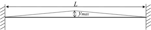
Figure 2. Free body diagram for a portion of the guitar string.

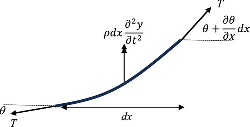
For small angles, the sine function terms in (1) can be approximated as $\sin \theta \approx \theta$ and $\sin \left(\theta +\frac{\mathrm{\partial }\theta }{\mathrm{\partial }x}\mathrm{dx}\right)\approx \theta +\frac{\mathrm{\partial }\theta }{\mathrm{\partial }x}\mathrm{dx}$. These approximations can be substituted into (1) and noting that, $\theta =\frac{\mathrm{\partial }y}{\mathrm{\partial }x}$, gives the wave equation, (2) $\frac{{\mathrm{\partial }}^{2}y}{\mathrm{\partial }{t}^2}=c^2\frac{{\mathrm{\partial }}^{2}y}{\mathrm{\partial }{x}^2}$(2) where $c=\sqrt{\frac{T}{\rho }}$.

The wave equation together with the initial conditions, (3) $y\left(x,0\right)=f\left(x\right)$(3) $\dot{y}\left(x,0\right)=0$ and boundary conditions, (4) $y\left(0,t\right)=y\left(L,t\right)=0$(4) gives a model for the simulation of a guitar string.

3.2. Solution to the wave equation

The wave equation for an initially stationary guitar string with the profile shown in Figure 1 has an analytical solution of the form, (5) $y\left(x,t\right)=\sum _{k=1}^{\mathrm{\infty }}{a}_k\sin \left(\frac{\mathrm{k\pi }}{L}x\right)\cos \left(\frac{\mathrm{ck\pi }}{L}t\right)$(5) where the coefficients, a_k are determined as (6) $a_k=\frac{2}{L}{\int }_0^{L}f\left(x\right)\sin \left(\frac{\mathrm{k\pi x}}{L}\right)\mathrm{dx}$(6) f(x) is the initial profile of the string at t = 0. For the piecewise continuous linear profile shown in Figure 1, (7) $a_k=\frac{8y_{\max }}{k^2{\pi }^2}\left\{\begin{array}{ll}1& k=2n-1,n\mathrm{is}\mathrm{odd}\\ 0& k=2n\\ -1& k=2n-1,n\mathrm{is}\mathrm{even}\end{array}\right\}$(7) the analytical solution (5) is the sum of an infinite series. From a practical view point, a finite series must be used.

The analytical solution, (5) is an idealised model, for example no energy dissipation is included. If a more realistic model is considered, then the derivation of an analytical solution is more difficult. If a more sophisticated model was considered, such as the modelling of a string as a thin beam, accounting for the stiffness of the string, or including energy dissipation (Devages, 2016) gives a model of the form, (8) $\frac{{\mathrm{\partial }}^{2}y}{\mathrm{\partial }{t}^2}=c^2\frac{{\mathrm{\partial }}^{2}y}{\mathrm{\partial }{x}^2}-C_D{\left(\frac{\mathrm{\partial }y}{\mathrm{\partial }t}\right)}^2-\frac{\mathrm{EI}}{\rho }\frac{{\mathrm{\partial }}^{4}y}{\mathrm{\partial }{x}^4}$(8) with initial conditions given as (3) and boundary conditions (9) $y\left(0,t\right)=y\left(L,t\right)=\dot{y}\left(0,t\right)=\dot{y}\left(L,t\right)=0$(9)

The point is that extending the analytical solution of (2) to the more sophisticated model (8) is not possible. Some more mathematical analysis is required to produce a new analytical solution for (8), which is beyond a mechanical engineer’s experience.

3.3. Application of the method of lines

A better way forward to searching for an analytical solution to a continuous model is to apply a numerical method to give an approximate solution where the accuracy is controlled by the timestep and space-step in the method. Should a more sophisticated continuous model be proposed then the extension of the numerical method should be relatively straight forward.

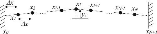
The numerical method of choice advocated in this paper is the semi-discretisation technique called the method of lines (Cash and Psihoyios, 1996). In the method of lines, the partial differential equation is approximated as a system of ordinary differential equations (ODE) that can then be solved using any numerical ODE solver. The semi-discretisation of the vibrating string model (2) is as given below. The guitar string is separated into N discrete lines as shown in Figure 3. The vertical displacement at the location of each line can then be represented as (10) $y_i\left(t\right)=y\left(x_i,t\right)$(10)

Figure 3. Division of a guitar string into N lines.

Substituting into (2) and approximating the second-order spatial derivative as a second-order central difference, $\frac{{\mathrm{\partial }}^{2}y}{\mathrm{\partial }{x}^2}=\frac{y_{i+1}-2y_i+y_{i-1}}{{\left(\mathrm{\Delta }x\right)}^2}+O\left({\left(\mathrm{\Delta }x\right)}^2\right)$ gives the system of ODEs, (11) ${\ddot{y}}_i=\frac{c^2}{\mathrm{\Delta }{x}^2}\left(y_{i+1}-2y_i+y_{i-1}\right),i=1,2,\dots ,N$(11) where Δx is the space-step, $\mathrm{\Delta x}=\frac{L}{N+1}$ giving a uniform spacing of lines and y₀ and y_N+1 are given by the boundary condition values (4).

The ODE numerical solver is formulated to solve first-order systems of ODEs. To solve the system (11) using an ODE solver it is converted from a second-order system with N dependent variables, $\left(y_i=1,2,\cdots ,N\right)$, to a first-order system with 2N dependent variables, $\left(y_i,{\dot{y}}_i,i=1,2,\cdots ,N\right)$. The first-order system must take the form: (12) $\dot{\mathit{Y}}=f\left(t,\mathit{Y}\right)$(12) where $\mathit{Y}=\left(\begin{array}{c}{Y}_1\\ Y_2\\ \cdots \\ Y_{2N}\end{array}\right)=\left(\begin{array}{c}{y}_1\\ y_2\\ ⋮\\ y_N\\ {\dot{y}}_1\\ {\dot{y}}_2\\ ⋮\\ {\dot{y}}_N\end{array}\right),\dot{\mathit{Y}}=\left(\begin{array}{c}{\dot{Y}}_1\\ {\dot{Y}}_2\\ \cdots \\ {\dot{Y}}_{2N}\end{array}\right)=\left(\begin{array}{c}{\dot{y}}_1\\ {\dot{y}}_2\\ ⋮\\ {\dot{y}}_N\\ {\ddot{y}}_1\\ {\ddot{y}}_2\\ ⋮\\ {\ddot{y}}_N\end{array}\right)$

The second-order system of ODEs, (11), is transformed into the first-order system, (13) $\dot{\mathit{Y}}=\left(\begin{array}{cc}0& I_N\\ A& 0\end{array}\right)\mathit{Y}$(13) where I_N is the NxN identity matrix and A is defined to be (14) $A=\frac{c^2}{\mathrm{\Delta }{x}^2}\left(\begin{array}{ccccc}-2& 1& 0& \cdots & 0\\ 1& -2& 1& 0& \cdots \\ 0& & \cdots & & 0\\ \cdots & 0& 1& -2& 1\\ 0& \cdots & 0& 1& -2\end{array}\right)$(14)

The identity matrix in (13) is introduced to reflect the structure of the first-order system, as ${\dot{Y}}_i=Y_{N+i},i=1,2,\dots ,N$. The matrix A is introduced to satisfy the right-hand side of the second-order system (11). The first-order ODE system can then be solved using an ODE solver based on a fourth-order and fifth-order Runge Kutta method (Press et al., 1992).

3.4. Animation of a guitar string

We are now in a position to numerically solve the guitar string model. As dynamics is about the movement of mechanical systems, it is insightful to see the solution in the form of an animation. The best way to implement this is as part of a GUI.

The GUI developed for investigating dynamics and music generation is shown in Figure 4. This is built using the GUIDE package as part of MATLAB (Dukkipati, 2009). The GUI is designed such that data is input relating to the string characteristics such as the length of the string, the tension in the string and the mass per unit length. Simulation parameters such as the simulation time in milliseconds, and the number of degrees of freedom are also in the GUI input data section. The GUI can also simulate the dynamics of a piano string and a violin string. As well as an animation of the respective stringed instruments other outputs can be generated such as the vibrating string trajectory at the centre of the string as a function of time. The GUI can also calculate and display the different natural frequencies of the continuous model and the equivalent for the semi-discrete model. The GUI can also simulate the sound of a vibrating string given its first natural frequency.

Figure 4. GUI for the simulation of music generation.

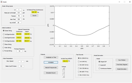
The GUI is a sophisticated tool for learning, its use will be illustrated below. For all animations, the string characteristics are set to L = 1 m, ρ = 0.4 g/m and T = 70 N. For the guitar string, the initial profile of the string is shown in Figure 1, with y_max = 0.01 m. In a paper it is impossible to show an animation other than presenting the string profile at a few different equally spaced times. Figure 5 shows the guitar string profile for a number of different times. For this simulation the number of lines, the string is divided into N = 20.

Figure 5. Guitar string profile for a number of times.

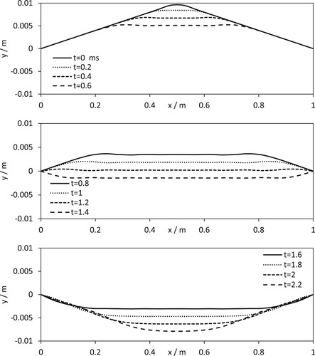
Figure 5 shows the vertical oscillation of the guitar string, with string profiles given at a time interval of Δt = 0.2 ms. Figure 5 also shows there is a finite time for the response of the guitar string at a given value of x based on the vertical propagation of the wave. Before the wave arrives, the string is stationary. Considering the string at a given value of x other than the midpoint, the behaviour can be split into a periodic motion consisting of two steady states that the string oscillates between.

4. Natural frequencies and eigenfunctions

To derive a relationship for the natural frequencies of the wave equation, a solution based on the separation of variables technique is applied. The analysis is given in Stephenson (1973). The general solution for the wave equation (2) is (15) $y\left(x,t\right)=\left(\mathrm{Asin}\left(\frac{\omega }{c}x\right)+\mathrm{Bcos}\left(\frac{\omega }{c}x\right)\right)\left(\mathrm{Csin}\left(\mathrm{\omega t}\right)+\mathrm{Dcos}\left(\mathrm{\omega t}\right)\right)$(15)

Imposing the boundary conditions (4) gives the conditions, B = 0 and $\mathrm{Asin}\left(\frac{\omega }{c}x\right)=0$. In general, A cannot be zero and satisfy the initial condition (3), therefore, the sine term must be zero. This gives the condition for determining the natural frequencies, (16) $\sin \left(\frac{\mathrm{\omega L}}{c}\right)=0\Rightarrow {\omega }_i=\frac{\mathrm{i\pi c}}{L},i=1,2,\dots$(16)

Converting to a natural frequency in Hertz, $f_i=\frac{{\lambda }_i}{2L}\sqrt{\frac{T}{\rho }},i=1,2,\dots$ For the semi-discrete approximation to the wave equation, there are N natural frequencies. The natural frequencies are related to the eigenvalues of the matrix A defined in (14). ${\lambda }_i=\mathrm{eig}\left(A\right),i=1,2,\dots N$ (17) $f_i=\frac{\sqrt{{\lambda }_i}}{2\pi },i=1,2,\dots ,N$(17)

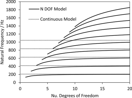
For L = 1 m, ρ = 0.4 g/m and T = 70 N, the natural frequencies for N = 1, 2, … , 10 are plotted in Figure 6. The first five natural frequencies for the continuous model are also plotted. From the figure, it is clear that the natural frequencies of the semi-discrete model as N increases tend towards the natural frequencies of the continuous model. For N = 20, for the parameter values defining the guitar string in the simulation shown in Figure 5 the difference in the first, second and third natural frequencies between the continuous model and the semi-discrete model is 2.5%. 2.8% and 3.2% respectively.

Figure 6. Natural frequencies versus Nu. degrees of freedom.

The eigenfunctions associated with each natural frequency can be used as initial conditions to yield some interesting behaviour. Figure 7 shows the behaviour of the simulated guitar string where the initial condition is the second and third eigenfunctions. Figure 7(a) shows the simulated guitar string profile for the second eigenfunction as the initial condition, (18) $y\left(x,0\right)=\sin \left(\frac{2\pi }{L}x\right)$(18)

Figure 7. Guitar string profile for a number of times for (a) second eigenfunction and (b) third eigenfunction.

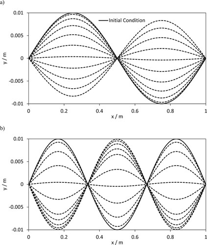
The guitar string profiles at t = 0.1 ms to 1 ms step Δt = 0.1 ms are also shown. The equal spacing in time of the guitar string curves indicates where the maximum acceleration occurs. Figure 7(b) shows a similar simulation with the third eigenfunction as the initial condition. In Figure 7(b), the initial condition together with 10 guitar string profiles for different time values separated by Δt = 0.1 ms are shown. Comparing Figures 7(a and b), it can be seen that as the third natural frequency has a higher frequency 607 Hz compared to the second natural frequency 407 Hz the guitar string in Figure 7(b) is moving more quickly than the guitar string in Figure 7(a). This can be inferred from the spacing between the guitar string profiles shown in Figures 7(a and b).

5. Simulating the motion of a piano string and a violin string

Any instrument that relies on a vibrating string to generate sound can be modelled by the wave equation (2) with appropriate initial conditions and boundary conditions.

5.1. Simulation of a piano string

The difference between the vibration of a piano string and a guitar string is a guitar string is plucked and a piano string is struck with a hammer. For a piano string, this creates a local distortion of the string as an initiation of the vibration. The wave equation (2) without modification is appropriate. The difference is the initial condition. For the piano string simulation discussed below, an initial condition of the form (19) $y\left(x,0\right)=f\left(x\right)=\{\begin{array}{ll}0& x<{\displaystyle \frac{L}{2}}-{\displaystyle \frac{\mathrm{\Delta }{x}_b}{2}}\\ {\displaystyle \frac{y_{\max }}{2}}\left(1+\cos \left({\displaystyle \frac{2\pi \left(x-\mathrm{\Delta }{x}_b\right)}{\mathrm{\Delta }{x}_b}}\right)\right)& {\displaystyle \frac{L}{2}}-{\displaystyle \frac{\mathrm{\Delta }{x}_b}{2}}<x<{\displaystyle \frac{L}{2}}+{\displaystyle \frac{\mathrm{\Delta }{x}_b}{2}}\\ 0& {\displaystyle \frac{L}{2}}+{\displaystyle \frac{\mathrm{\Delta }{x}_b}{2}}<x\end{array},\}$(19) is imposed where y_max  = 0.01 m and Δx_b = 0.1 m. This is a smooth pulse with a base, Δx_b and amplitude y_max. The analytical solution is given as (5) where the coefficients a_k are evaluated using (6). For the profile (19), the constants a_k are evaluated using numerical integration. To avoid a numerical integration of (6), a_k are evaluated analytically for a piecewise linear approximation to (19) with the same base and amplitude. For this profile, the constants, a_k are given as, (20) $a_k=\frac{8L{y}_{\max }}{k^2{\pi }^2\mathrm{\Delta }{x}_b}\sin \left(\frac{\mathrm{k\pi }}{2}\right)\left(1-\cos \left(\frac{\mathrm{k\pi }\mathrm{\Delta }{x}_b}{2L}\right)\right),k=1,2,\dots$(20)

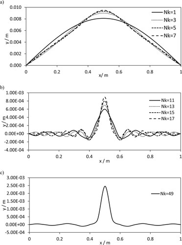
Figure 8 shows approximations to the initial condition for the guitar string and the piano string. In the analysis below, the initial condition for a piano string (19) is approximated to be a piecewise linear approximation. Figure 8(a) shows four approximate profiles for the guitar string initial condition with N_k = 1, 3, 5 and 7 terms in the series solution. From the figure, it is clear that the profiles tend to the initial condition with few terms in the series. This is not the case for the initial profile of a piano string approximated by a piecewise linear profile. In Figure 8(b), the approximate profile for the initial condition for a piano string is shown for the series solution with N_k = 11, 13, 15 and 17 terms in the series. Even with 17 terms in the series, the maximum amplitude at x = 0.5 m is far from y_max. Figure 8(c) shows the approximate initial profile for the piano string with N_k = 49 terms in the analytical series solution. This is included as it shows that for a piano string many terms are required to approximate the initial condition (19). Increasing the number of terms in the analytical solution for the piano string to N_k = 500, the relative error in the initial amplitude is 9%.

Figure 8. Approximate profiles for the initial condition for (a) a guitar string, (b) a piano string and (c) a piano string with 49 terms in the analytical solution.

Applying the method of lines to a piano string simulation the only issue is the number of subdivisions of the piano string. The base of the initial pulse for a piano string introduces a new length scale into the simulation compared to a guitar string that requires more subdivisions of the piano string to resolve. For the piano string discussed below, N = 500. The same string parameters as specified for a guitar string are used for the piano string, L = 1 m, ρ = 0.4 g/m and T = 70 N.

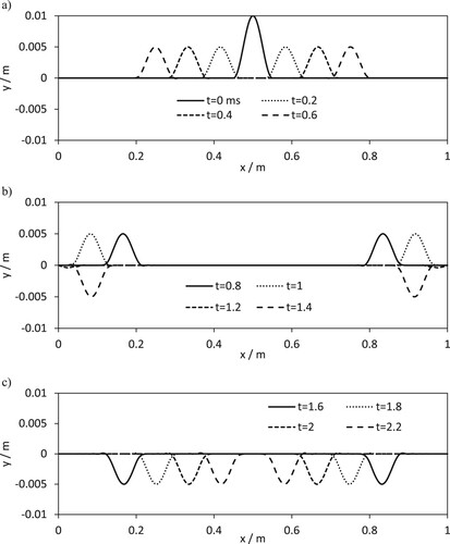
Figure 9 shows the piano string for a number of different times, calculated using the method of lines. The same time values are used as that for the guitar string simulation shown in Figure 5. The initial condition (19) gives an initial distortion located at the centre of the piano string. As time progresses the initial pulse separates into two waves with half the amplitude of the original pulse propagating away from the piano string centre. The waves travel at a speed of 419 m/s based on a travel distance between the wave peak at t = 0.4 ms and t = 0.6 ms. This should be compared with the theoretical wave speed of c = 418 m/s. At just beyond t = 1 ms, the two waves approach the boundary and are reflected at t = 1.2 ms to produce return waves with a negative displacement, propagating towards the centre of the piano string. For a time after t = 2.2 ms, the two waves coalesce at x = L/2 and the cycle repeats.

Figure 9. Piano string profile for a number of times.

5.2. Simulation of a violin string

The pattern of vibration of a violin string is complex compared to a guitar string or a piano string. The bow hair is coated with rosin to increase the coefficient of friction between the bow and the violin string. Music is generated with a violin using the stick-slip effect (Akar and Willner, 2020). As the bow traverses the violin string, at the point of contact with the bow the violin string goes through a two-stage cycle of the violin string sticking to the bow hair followed by the violin string moving backwards relative to the bows motion, the slipping stage of the cycle. During the stick stage, at the point of contact the violin string has the same speed as the bow. As the violin string is distorted by this process, the friction force increases until the maximum friction force is reached, (21) $F_f\le F_{f,\max }={\mu }_s{N}_{\mathrm{bow}}$(21) where F_f is the friction force, μ_S is the static coefficient of friction and N_bow is the reaction force on the string from the bow. Once the maximum friction force is achieved the violin string passes into the slip stage where the violin string accelerates towards the equilibrium position, sliding in the opposite direction to the movement of the bow. While the violin string slides relative to the bow the dynamic coefficient of friction determines the friction force. The violin string continues to slide relative to the bow until the relative velocity of the bow and violin string is zero and the cycle begins again (Devages, 2018).

As already stated, for a real violin string the vibrating motion is complex, with vibration occurring in both the vertical and horizontal direction. Our objective is to produce a model that qualitatively reproduces the motion of a violin string. To simplify the model, we will only consider; horizontal vibrations, the bow is positioned at the midpoint of the violin string and the sliding part of the cycle the dynamic coefficient of friction is taken to be negligible or equivalently the bow is lifted off the violin string. This is a legitimate technique for playing the violin called Spiccato (Thornton, 2021).

Under the above assumptions and taking the violin string to initially be undistorted gives the initial value problem, (2) together with the initial profile and boundary conditions, $y\left(x,0\right)=0,0\le x\le \frac{L}{2}$ $y\left(0,t\right)=0$ (22) $\dot{y}\left(\frac{L}{2},t\right)=V_{\mathrm{bow}}\mathrm{stick}\mathrm{stage}$(22) ${\frac{\mathrm{\partial }y}{\mathrm{\partial }x}|}_{\left(\frac{L}{2},t\right)}=0\mathrm{slip}\mathrm{stage}$

There is no analytical solution to the above set of boundary conditions that is derived easily. Applying the method of lines to the violin string model is discussed below.

The system of differential equations based on the method of lines is given as (11) with the values, y₀ and y_N+1 depending on the boundary conditions (22). The violin string displacement at x = 0 is zero, so the boundary condition is applied in the same way as for a guitar string or piano string. The boundary condition applied at x = L/2, the midpoint of the violin string the method of lines system is separated into two stages, the “stick” stage and the “slip” stage. Two parameters are also defined, t_st and y_st, and these are the time the stick stage starts and the distortion of the violin string at its midpoint when the stick stage is initiated. In the stick stage, the violin string at x = L/2 moves with the same velocity as the bow and (23) $y_{N+1}=y_{\mathrm{st}}+V_{\mathrm{bow}}\left(t-t_{\mathrm{st}}\right)$(23)

During the stick stage of the violin string vibration at x = L/2, the acceleration is zero. The horizontal components of the forces perpendicular to the string, acting at x = L/2 are in equilibrium, $2\mathrm{Tsin}{\theta }^{\ast }=F_f$ $\sin {\theta }^{\ast }=\frac{y_{N+1}}{\sqrt{\frac{1}{4}{L}^2+y_{N+1}^2}}$

The angle θ* is defined by approximating the violin string during the stick stage of the vibration cycle to have an approximate piecewise linear shape. As the violin string moves further away from the equilibrium position the angle θ* increases and the friction force must increase to equalise the forces in the horizontal direction perpendicular to the string. Once 2Tsin θ* exceeds the maximum friction force, F_f = μ_SN_bow the violin string transitions into the slip stage of the violin string motion. This is the simplest implementation of the detection of the transition from the stick stage to the slip stage of the violin string motion.

In the slip stage, the boundary condition at x = L/2 is (24) $y_{N+1}=y_N$(24)

The slip stage continues until the relative velocity between the violin string and the bow is zero. (25) ${\dot{y}}_{N+1}-V_{\mathrm{bow}}=0$(25)

When the relative velocity condition is satisfied the parameter t_st is set to the current time and y_st set to the displacement of the violin string at x = L/2, and the stage then changes back to the stick stage and the process is repeated. To start the cycle, it is assumed that the violin string is in the stick stage with t_st = 0 and y_st  = 0.

In the violin string simulation given below the string parameters are the same as used previously for a guitar string and a piano string, L = 1 m, ρ = 0.4 g/m and T = 70 N. The bow parameters are set to μ_S = 1.2, N_bow = 1 N and V_bow = 1 m/s.

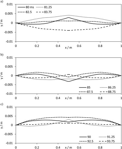
The half string domain is simulated with N = 100 lines, taking account of the symmetry is equivalent to N = 200 for the violin string. To give a student insight into the violin string motion using string profiles at different times is more difficult than for a guitar string or a piano string. It is not the initial condition that generates the sound, the violin string is forced, therefore rather than show violin string profiles close to the beginning of the simulation, violin string profiles are shown in Figure 10 for t =  80 ms through to 93.75 ms step Δt = 1.25 ms. In Figure 10(a) at t = 80 ms, the violin string is in the stick stage of the cycle. For t = 81.25 ms, the string is close to being at the maximum distortion and is about to move into the slip stage. The remaining profiles shown in Figure 10(a) demonstrate the rapid acceleration in the slip stage in the opposite direction to the bows motion. Following on from this in Figures 10(b and c), the violin string is in the stick stage up to t = 92.5 ms and is characterised by the slow movement of the violin string at the point of contact with the bow, x = L/2. Another more subtle feature of the violin string motion shown in Figure 10(b) is the propagation of transverse waves. In Figure 10(b), the transverse wave propagates away from the bow. The transverse wave is then reflected at the bridge of the violin and return to the centre of the violin string.

Figure 10. Violin string profile for a number of times.

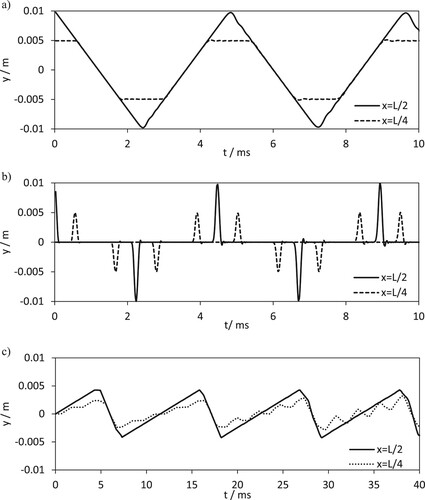
To see the transverse waves more clearly it is useful to plot the string displacement as a function of time at the centre of the violin string, x = L/2, and the point halfway between the string fixing point and the bowing point, x = L/4. Figure 11 shows the string displacement at these points as a function of time for a guitar string, a piano string and a violin string. Figures 11(a and b) show the predicted string displacement for a guitar string and a piano string respectively. These are included for reference purposes as particularly for the piano string it shows how the propagation of a transverse wave is characterised. In Figure 11(c), the time profiles for a violin string are shown. The simulation is over 40 ms rather than 10 ms as it takes some time for the violin string vibration to develop. The time profile at x = L/2 shows the stick-slip cycles of the violin string. The violin string profile at x = L/4 is indicative of transverse waves propagating away from and towards the middle of the violin string.

Figure 11. String displacement versus time: (a) guitar string, (b) piano string and (c) violin string.

The violin string model is idealised and can only be expected to qualitatively reproduce the dynamic motion of a violin string. In www.reddit.com, a slow motion video of a vibrating violin string is presented. In the video, the stick-slip cycle and the transverse wave propagation can be observed. The qualitative behaviour of the present simple violin string model is similar to that produced by the violin string model in Akar and Willner (2020). The violin string model in Akar and Willner (2020) is more sophisticated than the simple model presented here.

6. Conclusion

In this paper, continuous dynamic models are presented for a guitar string, piano string and violin string. The models are embedded in a GUI to make it possible for an engineering student to explore parameter space and the motion of a vibrating string using animation. It is shown how the different mechanisms for music generation translate into different boundary and initial conditions together with the wave equation.

Rather than solving the wave equation analytically, it is proposed to use a numerical solution technique. Analytical solutions exist for the simpler configurations in the form of infinite series solutions. The analytical solutions demonstrate the wave-like nature of the solution and allow the calculation of natural frequencies but are not easily extended to other more sophisticated models. Considering the numerical solution of the wave equation the numerical method of choice is the method of lines. The method of lines can be applied in a relatively straightforward way to more advanced vibrating string models. Should a more sophisticated model for the vibration of a string be implemented the changes to the numerical solution using the method of lines is relatively straight forward.

The derivation and simulation of continuous dynamic models are usually a topic in more advanced dynamic courses. The derivation of the wave equation uses constructs that engineering students taking introductory and intermediate courses in dynamics are very familiar with, such as free body diagrams. This means the subject matter is not totally foreign to engineering students taking introductory and intermediate courses in dynamics. Providing insight into advanced topics in dynamics for engineering students near the start of their undergraduate degree programmes is important. Insight into future topics in dynamics improves motivation giving a context to engineering students studies.

A further advantage of this investigation is vibrating string models make a strong connection with engineering students experience of listening to or playing music. The simulation of vibrating string models as part of a GUI provides an opportunity for a truly multimedia experiential approach to the teaching of a potentially very dry engineering science.

Disclosure statement

No potential conflict of interest was reported by the author.

References

- Akar, O., & Willner, K. (2020). Investigation of the Helmholtz Motion of a Violin String: A Finite Element Approach. ASME Journal of Vibration and Acoustics, 142, 1–11.
- Berry, J. S., Savage, M., & Williams, J. (1989). Mechanics in decline? International Journal of Mathematical Education in Science and Technology, 20(2), 289–296. https://doi.org/10.1080/0020739890200209
- Biggoggero, G. F., & Rovida, E. (1977). Problems in the teaching of mechanics, European J. European Journal of Engineering Education, 2, 277–290.
- Campo, A. (2022). The numerical method of lines facilitates the instruction of unsteady heat conduction in simple solid bodies with convective surfaces. International Journal of Mechanical Engineering Education, 50(1), 3–19. https://doi.org/10.1177/0306419020910423
- Cash, J. R., & Psihoyios, Y. (1996). The MOL solution of time dependent partial differential equations. Computers & Mathematics with Applications, 31, 60–78. ISSN: 0898-1221.
- Cumber, P. S. (2015). Waggling pendulums and visualisation in mechanics. International Journal of Mathematical Education in Science and Technology, 46, 611–630.
- Cumber, P. S. (2016). Waggling conical pendulums and visualisation in mechanics. International Journal of Mathematical Education in Science and Technology, 47, 612–636.
- Cumber, P. S. (2021). Visualisation in mechanics: The dynamics of washing machines. International Journal of Mathematical Education in Science and Technology, 52, 626–652.
- Cumber, P. S. (2022). The kinematics and static equilibria of a Slinky. International Journal of Mathematical Education in Science and Technology, 55(4), 1065–1083. https://doi.org/10.1080/0020739X.2022.2129498
- Cumber, P. S. (2023a). Lagrange’s method applied to a Slinky. International Journal of Mechanical Engineering Education, 1–29. https://doi.org/10.1177/03064190231191251
- Cumber, P. S. (2023b). There is more than one way to force a pendulum. International Journal of Mathematical Education in Science and Technology, 54(4), 579–613. https://doi.org/10.1080/0020739X.2022.2039971
- Devages, C. (2016). Linear string vibrations in musical acoustics: Assessment and comparison of models. Journal of the Acoustical Society of America, 140(4), 2445–2454.
- Devages, C. (2018). Physical Modelling of the Bowed String and Applications to Sound Synthesis [Doctoral dissertation]. University of Edinburgh. Edinburgh Research Archive. era.ed.ac.uk/handle/1842/31273
- Dukkipati, R. V. (2009). MATLAB for Mechanical Engineers. New Age Science, U.K.
- Graham, E., & Peek, A. (1997). Developing an approach to the introduction of rigid body dynamics. International Journal of Mathematical Education in Science and Technology, 28, 373–380.
- Graham, E., & Rowlands, S. (2000). Using computer software in the teaching of mechanics. International Journal of Mathematical Education in Science and Technology, 31, 479–493.
- Klarić, Š., Lockley, A., & Pisačić, K. (2023). The Application of Virtual Tools in Teaching Dynamics in Engineering. Tehnički Glasnik, 17(1), 98–103. https://doi.org/10.31803/tg-20220303040401
- Koay, S. T. (2022). The art of effectively teaching math to engineering. American Society for Engineering Education. Paper ID #35954, pp. 1–9.
- Kocsis, I. (2007). Applying animation in the teaching of mathematics for students of engineering. In P. Olajos, T. Tomacs, & E. Kovvacs (Eds.), Proceed. 7th Int. Conf. Applied Informatics Eger, Hungary, January 28–31 (Vol. 1, pp. 107–113). Eszterhazy Karoly College, Eger.
- Press, W. H., Teukolsky, S. A., Vetterling, W. T., & Flannery, B. P. (1992). Numerical Recipes in Fortran 77, 2nd Edition. Cambridge University Press. ISBN 0-521-43064-X https://websites.pmc.ucsc.edu/~fnimmo/eart290c_17/NumericalRecipesinF77.pdf.
- Reddy, S. C., & Trefethen, L. N. (1992). Stability of the method of lines. Numerische Mathematik, 62, 235–267.
- Rohendi, D., Wahyudin, D., & Wihardi, Y. (2019). Multimedia animation for mathematical application in engineering. Journal of Physics: Conference Series, 1402, 1–8. IOP Pub. https://doi.org/10.1088/1742-6596/1402/7/077065.
- Sazhins, S. S. (1998). Teaching Mathematics to Engineering Students. International Journal of Engineering Education, 14(2), 145–152.
- Schiesser, W. E. (1993). The numerical method of lines: integration of partial differential equations. Mathematics of Computation, 60, 433–437.
- Silva, P. H. O., Nardo, L. G., Martins, S. A. M., Nepomuceno, E. G., & Perc, M. (2018). Graphical interface as a teaching aid for nonlinear dynamical systems. European Journal of Physics, 39, 1–18.
- Stephenson, G. (1973). Mathematical Methods for Science Students, 2nd Edition. Longman.
- Thornton, B. (2021). Sequential Strategies for Teaching Spiccato. American String Teacher, 71(1), 23–27. https://doi.org/10.1177/0003131320976184
- University of Cambridge NRICH Programme. https://nrich.maths.org/6513.
- Wideberg, W. (2003). A graphical user interface for the learning of lateral vehicle dynamics. European Journal of Engineering Education, 28, 225–235.
- www.reddit.com. https://www.reddit.com/r/physicsgifs/comments/nc353m/violin_string_being_driven_by_a_bow_in_slow_motion.