Models, algorithms and performance analysis for adaptive operating room scheduling

Abstract

The complex optimisation problems arising in the scheduling of operating rooms have received considerable attention in recent scientific literature because of their impact on costs, revenues and patient health. For an important part, the complexity stems from the stochastic nature of the problem. In practice, this stochastic nature often leads to schedule adaptations on the day of schedule execution. While operating room performance is thus importantly affected by such adaptations, decision-making on adaptations is hardly addressed in scientific literature. Building on previous literature on adaptive scheduling, we develop adaptive operating room scheduling models and problems, and analyse the performance of corresponding adaptive scheduling policies. As previously proposed (fully) adaptive scheduling models and policies are infeasible in operating room scheduling practice, we extend adaptive scheduling theory by introducing the novel concept of committing. Moreover, the core of the proposed adaptive policies with committing is formed by a new, exact, pseudo-polynomial algorithm to solve a general class of stochastic knapsack problems. Using these theoretical advances, we present performance analysis on practical problems, using data from existing literature as well as real-life data from the largest academic medical centre in The Netherlands. The analysis shows that the practically feasible, basic, 1-level policy already brings substantial and statistically significant improvement over static policies. Moreover, as a rule of thumb, scheduling surgeries with large mean duration or standard deviation early appears good practice.

Keywords:

• operating room scheduling
• adaptive scheduling
• stochastic knapsack problem
• operations research in healthcare

1. Introduction

Globally, the demand for health services increases as societies advance economically and populations age. This holds particularly true for the demand for hospital services, and hence for the surgical services provided in operating rooms (ORs). The services provided in ORs form a primary source of hospital revenue and drive a large share of hospital costs (Denton, Viapiano, and Vogl 2007; Cardoen, Demeulemeester, and Beliën 2010). As a result, the planning and scheduling of ORs are continuous and high priority activities in many hospitals around the globe. OR planning and scheduling have also received considerable attention in scientific literature, as demonstrated by the review of Cardoen, Demeulemeester, and Beliën (2010), which has identified 246 publications, among which 114 in the first decade of the present millennium. Other comprehensive reviews which address OR scheduling are provided by Erdogan et al. (2011), Gupta (2007), Gupta and Denton (2008) and Cayirli and Veral (2003).

In this work, we consider the scarcely researched common practice of making adaptations to the surgical schedule while schedule execution is in progression (May et al. 2011). Evidence shows that the stochastic nature of the operating room processes causes the effectiveness and efficiency of operating room performance to be importantly impacted by such adaptation decisions (Stepaniak, Mannaerts, et al. 2009). Aiming to contribute to practical performance improvement, we first develop required scientific models and algorithms, and subsequently analyse resulting improvement obtained for real-life problems. From the perspective of the operating room scheduling classification scheme of Cardoen, Demeulemeester, and Beliën (2010), the presented research thus addresses operating room uncertainty.

Strategic planning is commonly considered as the highest level in hierarchical production planning frameworks, as is also the case in hospital production management (Vissers, Bertrand, and De Vries 2001). At the strategic level, hospital management decides which specialties to offer, how many operating rooms to run and on capital intensive equipment. At the next lower level, the tactical level, hospital management divides the resulting operating room capacity, often in the form of periodic rosters which specify slots (or blocks) of operating room time to specialties or individual doctors. For instance, Orthopaedics may get surgery time assigned every Monday from 8 am to 4 pm in room 2. At the subsequent operational level, specialties or doctors select for each slot which patients to operate, in alignment with the operating room planners. Prior to the day of operation, the final operating room schedule typically specifies a sequence in which the selected patients will be treated, as well as expected start and end times for each patient. The stochastic, uncertain nature of surgical operations causes the schedules to often require adaptation while being in execution. This brings us at the executional, bottom, level of the production planning hierarchy.

Our work focuses on making optimal use of adaptivity, at the scheduling level and at the execution level. Because in practice adaptations are often confined to the slots assigned to a specialty or individual doctor, we develop models and methods within the context of a single operating room on a single day. Within such a slot, some of the scheduled surgeries may require much more time, others may take much less time, patients are cancelled as they are unfit for surgery, emergency patients may have to be inserted into the schedule, et cetera. Such events may lead to adaptations in the form of changes in schedule times, order, deletion, insertion, and addition of patients, and of cancelling patients at the end of the day. More precisely classifying the presented research in terms of the classification scheme of Cardoen, Demeulemeester, and Beliën (2010), we consider the problem of scheduling elective and emergent patients (field patient characteristics) assigned to a single operating room (field decision delineation) using exact combinatorial methods (field research methods), and test our methods on two real data-sets of empirical origin (field applicability of research).

The review by Cardoen, Demeulemeester, and Beliën (2010) already demonstrates that much scientific progress has been made at various of the aforementioned planning levels to improve operating room performance. Moreover, further recent research to better cope with uncertainty is provided by Tang and Wang (2015) who consider the tactical planning problem of robustly allocating limited operating room capacity to subspecialties so as to provide timely and accessible treatment. Another tactical problem is considered by Dellaert, Cayiroglu, and Jeunet (2016), who strive to balance waiting time and resource utilisation. Jebali and Diabat (2015) consider a problem of a more operational nature, namely to select elective surgeries, while considering uncertainties related to surgery duration as well as patient length of stay in the ICU and the ward.

Despite adaptations being common practice, it has however received little attention in the scientific literature. Zhou et al. (1999) and Dexter et al. (2004); Dexter, Willemsen-Dunlap, and Lee (2007) address deterministic solution approaches and analyse methods to construct a priori schedules using historic average durations as expected surgery durations. These authors show that solving the resulting static deterministic OR scheduling problems may result in poor OR utilisation and high patient waiting times. A natural subsequent improvement is to consider static stochastic approaches, as proposed in Denton, Viapiano, and Vogl (2007) and Batun et al. (2011). These authors propose one stage programmes, or two stage stochastic programmes with decisions taken in the first stage. Alternatively, Shylo, Prokopyev, and Schaefer (2012) propose a chance-constrained-based approach which minimises idle time while constraining the probability of overtime work. Wang, Tang, and Fung (2014) consider a chance-constrained model for a closely related problem with multiple operating rooms. van Oostrum et al. (2008) and Van Essen et al. (2014) also use chance constraints, and focus on the impact of the OR schedule on ward occupancy and overtime. These stochastic models capture important practically relevant uncertainties of OR scheduling.

All of the aforementioned work however considers the problem as static, or off-line, and disregards the common practice of adapting a priori schedules as the day proceeds (May et al. 2011). A first study which includes such adaptations is the simulation study by Stepaniak et al. (2012), who analyse the impact of risk attitudes of schedulers on their adaptation decision-making and the resulting operating room performance. Another simulation study which analyses adaptive policies is provided by Vermeulen et al. (2009), who consider a planning problem arising in the context of allocating CT scan capacity over different patient groups. Zhang, Xie, and Geng (2014) investigate dynamic allocation of surgeons/surgeries to multiple operating rooms. In contrast to the problem we study however, their model assumes that all selected patients must be treated. More closely related is the recent work of Xiao et al. (2016) who solve a version of the problem where adaptation is allowed only once per day, using a computationally intensive three-stage stochastic recourse model. We also refer to their work for a general discussion of the connection between stochastic OR scheduling and the stochastic scheduling literature. For the OR scheduling literature, a general analytic approach towards adaptivity in operating room schedules is lacking in the scientific literature, despite being common practice.

Our main contributions are twofold. First, we develop adaptive models and solution methods for single day single operating room scheduling problems and present theoretical results on their relative performance. Second, we show that adaptive policies can substantially improve over non-adaptive policies in practice, using two real-life data-sets from Erasmus Medical Center (one of which is available via scientific literature). We reflect on practically relevant insights and guidelines in the discussion and conclusions.

2. Embedding in adaptive scheduling literature

Ilhan, Iravani, and Daskin (2011) consider adaptive policies for a knapsack problem with deterministic weights and stochastic rewards. The single operating room scheduling we consider in this paper differs from their problem as it has stochastic weights and deterministic rewards. Adaptivity has also been widely studied for settings with weights that are unknown until the item is inserted in the knapsack, and where items are added one by one until the capacity is exceeded. In such problems, it is often assumed that all items added until capacity is exceeded contribute to total reward (Dean, Goemans, and Vondrák 2008; Bhalgat, Goel, and Khanna 2011; Levin and Vainer 2013; Balseiro and Brown 2016; Blado, Hu, and Toriello 2016), or that exceeding the capacity of the knapsack results in a final reward of zero (Chen and Ross 2014). In accordance with operating room scheduling practice, we model exceeding capacity using overtime penalties (cost).

Because adaptive problems are of a recursive nature, their solution can be computationally demanding. To help control computation times, Ilhan, Iravani, and Daskin (2011) introduce the concept of l-level adaptivity, and propose and analyse corresponding l-level heuristics. l-level adaptivity is defined by restricting adaptation to the time of completion of the next l jobs (viz. patients). We adopt the l-level adaptivity framework of Ilhan, Iravani, and Daskin (2011), yet translate it to the setting of stochastic weights and costs for overtime, and to the practice of operating room scheduling.

In operating room scheduling, it is not desirable to adapt schedules instantly. Both for technical reasons and for reasons of patient-centeredness, it is considered infeasible to decide on the next patient to schedule immediately after a surgery on a current patient has finished. Typically, the sequence of next patients to be scheduled is committed one or more patients ahead. To model this practical requirement, we introducing the concept of committing, i.e. to consider the schedule for subsequent patients as partly fixed. More specifically, k-level committing is defined as prohibiting adaptations to the sequence of the next k patients in the schedule, after which an l-level policy allows adaptations for the next l decisions.

The core of any l-level adaptive policy for the knapsack problem is formed by an exact algorithm for the corresponding static knapsack problem. In our case, the static problem refers to the version of the problem where all patients are selected and sequenced at the beginning of the day, and adaptations are not allowed. Merzifonluoğlu, Geunes, and Romeijn (2012) study static policies for a knapsack problem with stochastic weights and rewards, and a penalty for exceeding the knapsack capacity. Their analysis assumes normally distributed weights. Computational results on stochastic knapsack problems with normally distributed item sizes or rewards are also presented in the seminal work on sample average approximation by Kleywegt, Shapiro, and Homem-de Mello (2002). To support their l-level heuristics, Ilhan, Iravani, and Daskin (2011) develop an algorithm for the static problem with normally distributed rewards and deterministic weights.

In the setting of OR scheduling, evidence shows that the normal distribution fits empirical surgery durations relatively poorly because of its positive skew (Stepaniak, Heij, et al. 2009). In Section 4, we develop a new pseudo-polynomial algorithm to solve the static stochastic version of our problem to optimality and which forms the core of the subsequently analysed adaptive policies. It solves the static stochastic knapsack problem for a general class of problems where the distributions of the weights fall into the class of additive distributions. The normal distribution falls into this class.

The problem objective under consideration (classification field performance measures) is rooted in the work of Dexter, Macario, and Traub (1999), Dexter et al. (1999) and Stepaniak et al. (2012) who aim to balance the advantages and disadvantages of performing surgeries in overtime. More specifically, we consider the problem of maximising the rewards which result from providing surgical services to patients selected from a given set, minus the corresponding cost of working overtime. Rewards and costs are not only to be understood in terms of hospital revenue and operating costs, but may also include health benefits, patient satisfaction and employee satisfaction. As outlined by Stepaniak et al. (2012), overtime work may result in higher labour costs and cause job dissatisfaction and employee turnover among OR staff. On the other hand, delay of surgery to the next day or beyond may result in patient dissatisfaction, patient anxiety, longer recovery (perhaps with worse outcomes) and ultimately, loss of health. Obviously, policies which allow more generous adaptation (l-level adaptivity with large l in combination with low k-level committing) provide more opportunity for cost-efficient solutions and to reduce cancellations. Such policies, however, may increase dissatisfaction and anxiety from patients who have less certainty about their surgery (time). The presented analysis and results do not mean to disregard such dissatisfaction and anxiety, but provide insight in the gains which can be made through adaptive scheduling with committing, where the committing level can be set to control dissatisfaction and anxiety. We explicitly reflect on the practical considerations and implications in the discussion and conclusions.

3. Models for studying adaptive OR scheduling

We now present our models for single day single room adaptive scheduling. The models assume a fixed set of patients from which to select and schedule patients for surgery. Typically this is the set of patients initially selected by the specialty or surgeon, perhaps added with reserve patients and acute recent arrivals. The task is to select patients for surgery from this set, and provide a treatment sequence for the selected patients. The objective function will count a deterministic reward for each patient treated at the end of the day. The patient rewards can depend on condition, but also on urgency, or for instance be higher for patients which got cancelled the previous day(s). Further, the objective function charges a penalty per time unit overtime. Overtime occurs when the sum of surgery durations of selected patients exceeds the (given) regular working time. Surgery durations are random variables, whose value is unknown until surgery is completed. However, the stochastic distribution functions describing the surgery durations are known beforehand. Hence expected overtime costs for a given selection of patients can be calculated on beforehand.

A static policy selects and sequences all patients at the beginning of the day, and does not make adaptations to the selection or sequence as the surgeries are executed and actual surgery durations become known. An adaptive policy, by contrast, may adapt the selection and/or sequence as surgeries are completed and surgery durations of treated patients become known. Hence, unlike static policies, adaptive policies can take the actual duration of completed surgeries into account. Our main goal is to study the objective function values attained by various adaptive policies, especially in relation to objective function values attained by static policies. The objective function measures OR performance.

Because it may not always be feasible or desirable in practice to select the next patient at the time of completion of the current surgery, we introduce the concept of committing. An adaptive policy with k committings commits k patients for, meaning that no adaptations are allowed to first k patients in the sequence. Furthermore, whenever a surgery is finished, and committed patients remain, a next patient is added to the committed sequence, so that the committed sequence again consists of k patients. The simplest case of committing is an adaptive policy with 1 committing. It always selects the next patient at the start of the surgery of the current patient, and this patient must thus be treated next, regardless of the surgery duration of the current patient.

In the remainder of this section, we provide a detailed description of the above. In Section 3.1, we detail the patient set and reward structure, and in Section 3.2 we detail the various patient selection policies (static, adaptive, adaptive with committings).

3.1. The patient set and objective function

The patient set is partitioned into m subsets, called classes. A class corresponds to a single surgical procedure, e.g. hip replacement, or a set of homogenous surgical procedure types, e.g. acute trauma of the lower extremities. We denote by the number of patients at the beginning of the day for class i () and denote its corresponding vector . We denote by the random surgery duration of patient in class i. As said, we assume the distribution of to be known, but the actual duration to be revealed upon completion of surgery on the patient. Each surgical duration is independent of all other surgical durations. The surgical durations of patients within the same class follow the same distribution. Thus within class i, the random variables for are independent and identically distributed.

The more patients selected and receive surgery, the higher the hospital revenue and (or) the more patients enjoy the resulting health benefits. This is modelled by a reward contributed for each patient within class i for which surgery is completed by the end of the day. At the same time however, selecting many patients increases the likelihood of overtime, which is associated with increased risk on adverse events, patient dissatisfaction, employee dissatisfaction and overtime costs. Overtime occurs when the sum of the durations of completed surgeries exceeds the regular opening time of the OR . In the practical context of Erasmus Medical Center for instance, equals 450 min. Overtime cost is calculated using a standard price p per time unit overtime work (as in Denton, Viapiano, and Vogl 2007; Batun et al. 2011).

The yield (or net reward) is defined as the sum of the rewards of the patients for which surgery has been completed at the end of the day (including overtime) minus the overtime costs. Note that overtime is a random variable because surgery times are random variables. Moreover, for adaptive policies the selection of patients for which surgery is completed at the end of the day is dependent on the actual surgery times. Thus yield is also a random variable. As we are interested to maximise yield, and yield is a random variable, we choose the expected yield as objective function of our single day single operating room adaptive scheduling problem.

Note that the worst case expected overtime costs for treating a patient of type i is . This worst case occurs when the entire surgery takes place during overtime. Thus, would imply that all class i patients are always selected in any optimal solution. We assume to avoid this uninteresting and unrealistic case.

3.2. Patient selection

In this section we discuss the static and adaptive policies in more detail.

3.2.1. The static problem

Static policies may take the stochasticity of durations into account, but they disregard making adaptations to the patient selection or sequence as execution of the schedule progresses. Now, let denote the optimal solution value of the static problem and therefore be the maximum expected yield attainable by a static policy. More generally, for future use, we define as the optimal solution value for the static problem in which there are t time units and patient vector remaining, , , . A formal model for the static problem is now defined by (1) (2) (3) (4)

Here, if and only if the j-th patient of class i is selected for surgery. Since all patients within a class are identical, we may impose without loss of generality (WLOG) that per class, patients are selected in decreasing order of index. This is enforced by (3(3) ).

To address the complexity of the static problem, let us consider the special case where all surgical durations are deterministic (have variance zero), with for , and . Then any optimal solution for this problem will have . When , for , the (decision version of the) problem is then equivalent to the well-known knapsack problem, and therefore (weakly) NP-Complete (see Garey and Johnson (1979) and the references therein). Hence, we may conclude that the static problem is NP-hard.

We next introduce notation for the static policy with side-constraints: some patients must be scheduled. This is not a situation that will be studied in this paper: We introduce the notation because it will be convenient in subsequent sections. Let . Then define(5)

as the maximum expected yield obtainable under a static schedule with remaining time t and available patient vector , with the constraint that for each class at least patients must be scheduled.

3.2.2. The adaptive problem

We now formalise the model and notation for the adaptive problem. The adaptive problem is most naturally formulated via a dynamic programming formulation. Indeed, observe that after each surgery completion, the state of the system consists in the number of time units t remaining () and the number of untreated patients of each type remaining (). Let denote the maximum expected yield attainable via an adaptive policy in this state.

In each state, the choice is whether to treat another patient, and if so, from which class. Let denote the classes of patients available for surgery for patient vector . In each class, we again assume WLOG that patients are selected in decreasing order of index, implying that patient is the candidate patient in class . Thus, when selecting a patient in class , we move from state to state and obtain a reward . Here denotes the i-th standard unit vector. This gives rise to the following recursion:(6)

That is, in each step, we either select the patient that maximises our expected reward, or we select no more patients. If , then set for any f(i). Note that in (6(6) ), instead of incurring overtime costs after completing each patient, overtime costs are incurred for the entire overtime period when we decide to admit no more patients.

For any state , the optimal solution for the adaptive problem forms an upper bound on the maximum expected yield attainable by any adaptive policy for the corresponding problem. We refer to adaptive policies which are guaranteed to attain this upper bound as exact adaptive policies. Such exact adaptive policies have associated yield . Adaptive policies which do not necessarily deliver solutions having expected value are henceforth referred to as heuristic adaptive policies.

3.2.3. The adaptive problem with committing

The adaptive problem defined in Section 3.2.2 allows to select the next patient to undergo surgery after surgery on the previous patient completes. As argued in Section 1, this is not necessarily realistic. Instead, one may wish to commit one or several patients for surgery in advance. The recursion below formally models the arising adaptive problem where k patients are committed in advance.

To introduce a formulation with committing, we let denote the queue of committed patients. A patient of class is thus committed to undergo surgery next, and then a patient of class , etc. Let denote the number of patients of class i that are in the queue , we thus have . denotes the vector of untreated patients: There are untreated patients in class i that are not in queue to be treated. When selecting the next patient i to add to the queue, we must thus select .

We let denote the maximum expected yield for the adaptive problem with k committings, where patient vector and t time units are remaining, and the queue of committed patients is . (We will often omit the subscript of the first coordinate c of to improve legibility in formulas.) The following recursion then characterises the problem:(7)

So, given the state , we either commit a patient i and treat patient c, transiting to state and collecting a reward , or we may decide to commit no further patients, and to finish the surgery on the committed patients to obtain a reward (cf. (5(5) ) in Section 3.2.1).

Let denote the expected yield of the optimal adaptive policy with k committings. At the beginning of the day, we need to either find the optimal queue such that , or we need to use a static policy with fewer than k patients. We obtain:

Note that there is no need to impose that fewer than k patients are selected in the static alternative : If it is optimal to select more than k patients in the static policy, then .

4. Analysis of adaptive policies

In this section, we use the concept of l-level adaptivity to develop effective and computationally efficient heuristic adaptive policies (with and without committing). These adaptive policies will rely on efficient solution approaches for the static problem to overcome the computational difficulties of solving the adaptive problems as such. The concept of l-level adaptivity was introduced by Ilhan, Iravani, and Daskin (2011) for a knapsack problem with deterministic weights and stochastic rewards. We adapt the concept to our setting with stochastic weights and deterministic rewards and extend it to the case with committing. For this new setting, we derive results along the lines of results in Ilhan, Iravani, and Daskin (2011) and subsequently extend them to the case with committing. Moreover, we derive new monotonicity results on the impact of committing.

The l-level adaptive policies are introduced in Section 4.1. Section 4.2 presents monotonicity with respect to the number of committed patients.

4.1. A tractable adaptive policy

The l- level adaptive policy is defined recursively. The 0-level adaptive problem is the static problem. The 1-level adaptive problem is now informally defined as the problem of maximising expected yield by selecting a first patient, and solving the problem which remains upon completion of this first patient as a 0-level adaptive problem, i.e. as a static problem. Notice that the 1-level problem is adaptive as, by definition, it takes the realisation of the surgery duration time of the first patient into account in the selection and sequence of subsequent patients. The l-level adaptive policy refers to the problem of selecting a first patient, and solving the problem which remains upon completion of the first patient as an -level problem. More formally, denoting by the expected yield of the l-level adaptive problem in state , we obtain:(8)

This can be generalised as follows to the l-level adaptive problem with k committings we obtain:(9)

where and . At the beginning of the day, the reward attained by this latter policy is thus:(10)

As l-level problems only consider the realisations of surgery duration for the first l patients, they can be viewed as a hybrid between the adaptive problem and the static problem. The following result is along the lines of a similar result in Ilhan, Iravani, and Daskin (2011) and generalises that result to the case with committings:

Theorem 1

For any remaining time t, patient vector , committed patient vector , and for , it holds that

and for policies without committing and , it holds that

For all proofs, see Appendix 1. Theorem 1 shows that l-level adaptive policies outperform -level adaptive policies. Hence, it is preferable in practice to use the largest l which is computationally feasible.

Now, repeated application of l-level policies entails to solve the problem which arises after each surgery as an l-level problem, rather than using an l-level problem for selecting the first patient, and an -level problem for the second patient, etc. In this approach, in each state a patient is selected from the class that attains the maximum in (8(8) ) (or (9(9) ) for committing). Repeatedly selecting patients in this fashion is a policy that results in an expected yield for each state , and we denote this expected yield by (or for committing). The following theorem supports the use of this policy. It generalises a result in Ilhan, Iravani, and Daskin (2011) to the case with committing:

Theorem 2

For any remaining time t, patient vector , committing vector , and adaptivity level , it holds that and .

4.2. The impact of committings

This section regards the maximum expected yield attainable in adaptive problems with committing as a function of the number of committed patients. The following theorem shows that both for the adaptive problem, and for the l-level adaptive problem, the maximum attainable expected yield decreases with the number of committed patients.

Theorem 3 (Committing deteriorates performance)

Let with and consider committing vectors and . Then, for any time t, patient vector such that , and adaptivity level it holds that Moreover, for the optimal policy it holds that:

From this result, it follows easily that the maximal attainable reward at the beginning of the day decreases in the committing level. Intuitively, these results follow from the fact that the more patients are committed, the less room remains for optimisation in the adaptive selection of subsequent patients.

In summary, this section introduces adaptive policies and showed that in expectation they deliver better solutions than static policies. However, the l-level adaptive policies we developed frequently call an exact static policy. This is only computationally feasible for practical purposes, when the exact static policy is very efficient. The next section develops such an exact static policy for a broad class of surgery duration distribution functions.

5. A pseudo-polynomial algorithm for the static stochastic knapsack problem

As discussed in the introduction, the literature presents various solution approaches to stochastic knapsack problems. Merzifonluoğlu, Geunes, and Romeijn (2012) provide a branch and bound approach for the case with normally distributed weights and deterministic rewards. In the context of OR scheduling, however, Stepaniak, Heij, et al. (2009) have found that the symmetric normal distributions do not fit surgical durations well, and demonstrate that other distributions such as the lognormal distribution provide a significantly better fit. Below, we present a new, exact, pseudo-polynomial algorithm to solve the (static) stochastic knapsack problem, which applies to a general class of distributions and includes the normal distribution as a special case. The presented approach extends the well-known pseudo-polynomial dynamic programming solution method for the deterministic knapsack problem. As this dynamic programming algorithm is not a main contribution of this paper, we will not present explicit computational analysis in Section 6. However, the computational analysis evaluates the 1-level adaptive policy, which makes frequent calls to the dynamic programming algorithm. These results confirm the computational suitability of our method.

Definition 1

Let random variables be independently distributed, with having probability density function , then is closed under addition iff , .

This assumption captures a broad class of random variables. Unfortunately, the lognormal distribution advocated by Stepaniak, Heij, et al. (2009) for modelling surgery durations is not captured by this assumption. But we show in Section 6.1 and in the appendices that a class of random distributions satisfying 1 can be constructed that fits the empirical data rather well, confirming the flexibility and suitability of the assumption.

Parameters can be single valued, e.g. specifying the parameter in a Poisson distribution, or vector valued, e.g. specifying the mean and variance for normal distribution, which are both closed under addition. We now present a pseudo-polynomial solution method for the static problem for the case where the probability density functions are closed under addition and all parameter values are integral. The integral requirement can be relaxed by scaling techniques as used in Section 6.

Let represent the service time of the jth patient in class i and . Let be defined as in Definition 1. For any given parameter , let be the maximum reward over all subsets of the set of patients such that . Let denote the similarly defined objective function value. Then formally and can be defined as follows:(11) (12)

where , if there is no feasible solution to formula (11(11) ), define .

Notice that is a multidimensional Knapsack problem because of being closed under addition. We now present a dynamic programming formulation for and .

Theorem 4

For any parameter , and state , , with .

Theorem 4 implies that for any , can be found by solving the multidimensional Knapsack problem . We now briefly address how to solve for the problem under consideration where there are m patient classes with patients .

Definition 2

For any , let be the maximum reward over all subsets of patients such that , , . Moreover, we let if for all subsets of .

Introducing as the largest element in set , which indicates the class with largest index in , can now be recursively defined as follows:

Theorem 5

For any and ,(13)

The recursion in the theorem can be interpreted to repeatedly consider selection of the patient with the largest index in class and proceed to state if the patient is scheduled or to state otherwise. The recursion ensures the sequence assumption in Section 3.

Figure 1. Dynamic procedures.

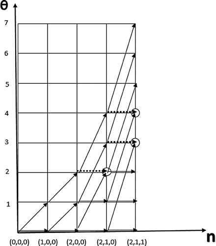
Figure 1 illustrates the dynamic programming recursion. It considers an example: there are three classes of patients with parameters , , , and the rewards are , , , respectively. The node corresponding to state ((0, 0, 0), 0) forms the origin of the state space, and the transitions are depicted by arcs. If a state space node has two incoming arcs, the solid arc represents the arc maximising the reward.

From Figure 1, we can also understand how to find . For each state , and the corresponding optimal subset of patients can be determined using dynamic programming. Moreover, for this subset of patients , , where can be calculated. The optimal solution can then be found by maximising over all , . This procedure can be extended to the case of committing, as the committed patients can simply be accounted for by setting . Through this an optimal track is derived to arrive at state if it is feasible and to get maximum objective value

Further, we notice that the presented approach is polynomial in the number of patients, but not in the input size of the problem if it is efficiently encoded. This is due to the fact that the presented problem with multiple patients per patient class is in fact a high multiplicity scheduling problem, see for instance Hochbaum and Shamir (1990, 1991). Hence, policies which iteratively select patients by applying a pseudo-polynomial algorithm can be classified as a pseudo-polynomial list generating algorithm (Brauner et al. 2005).

6. Computational results

In this section, we investigate various policies. We introduce acronyms below:

StS	=	Exact static policy (Section 3.2.1);
ANC	=	Exact adaptive policy (Section 3.2.2);
AOC	=	Exact adaptive policy with one committing (Section 3.2.3);
1-ANC	=	Repeated exact 1-level adaptive policy (Section 4.1);
1-AOC	=	Repeated exact 1-level adaptive policy with one committing (Section 4.1).

We let denote the corresponding expected yield. E.g. denotes the expected yield provided by an exact static policy. Because the 1-level adaptive policies are computed along a sample path, the expected yields and are estimated using Monte Carlo simulation with 2000 samples. We perform benchmarks using data from Van Houdenhoven et al. (2007) and from recently collected data, both originating from Erasmus Medical Center. We refer to the data Van Houdenhoven et al. (2007) as vHOHWK, and to the recently collected data as EMC. The benchmarks compare:

• The improvement of ANC and AOC over StS;

• The performance of 1-ANC and 1-AOC, when compared to ANC and AOC;

• The computational efficiency of 1-ANC and 1-AOC compared to ANC and AOC;

• Typical sequences in which patients from various classes are scheduled;

• The values of 1-ANC and 1-AOC in practice, using data from Erasmus Medical Center.

6.1. Description of test cases

The experiments fit surgery time using a class of finite parameter compound Poisson distributions (see Appendix 2 in the electronic companion appendix). The distributions are additive (as in Definition 1), asymmetric and non-negative, unlike the normal distribution. Moreover, they fit closer to the empirical data than chi-squared and fixed-scale Gamma distributions. We construct four low-dimensional cases consisting of three patient classes: Two based on the data from vHOWK and two based on the more recent data obtained directly from Erasmus Medical Centre. Additionally, we construct 4 high-dimensional cases based on the more recent data from Erasmus Medical Centre. Summarising statistics are given in Table 1. The table includes information on the average coefficient of variation (CV) of the surgery distributions in the class. The CV is defined as the standard deviation divided by the mean. For detailed information on the surgery time distributions for each patient we refer to Appendix B.2. A verification of the goodness of fit of the surgery time distributions with respect to the Erasmus Medical Center data is presented in Appendix B.3.

Table 1. Average coefficient of variation (CV) and number of patient classes for each case.

Low-dimensional cases			High-dimensional cases
Case name	Avg. CV	# of patient classes	Case name	Avg. CV	# of patient classes
vHOHWK-HCV	0.86	3	Ophthalmology	0.31	6
vHOHWK-LCV	0.76	3	Gynaecology	0.35	9
EMC-HCV	0.31	3	Orthopedics	0.29	10
EMC-LCV	0.19	3	Urology	0.24	12

For all cases, daily regular capacity is set at 450 min (7.5 h). W.l.o.g., we may rescale the unit overtime cost p to 1. We let rewards depend on mean and standard deviation of the surgery time distribution for class i by setting . We investigate a total of 15 combinations of to determine sensitivity: each and , but with omitted because for some of the patient classes in the test cases, this combination does not satisfy .

6.2. The performance of the 1-level adaptive policies

In the following, we investigate the performance of the 1-level adaptive policies 1-ANC and 1-AOC. As benchmarks, we use the optimal adaptive policies ANC and AOC, respectively. These latter policies are computationally tractable only for small numbers of patient classes, and we thus use the low-dimensional cases (see Table 1) to perform the benchmarks. The parameters are varied over 15 combinations, see Section 6.1. We consider patients per class, giving 3p patients in total. We perform a full-factorial experiment, resulting in a total of (4 cases values for value for test instances.

The quantities and have been termed benefit of adaptivity (Dean, Goemans, and Vondrák 2008). Define the relative benefit of adaptivity (rBoA) as (no committing), and as (one committing). Because and by Theorem 1, the 1-level adaptive policies capture a fraction of the maximal benefit of adaptivity. We now first investigate the total benefit of adaptivity for our test instances, and then assess which fraction of this benefit is captured by the heuristic 1-level adaptive policies. Table 2 gives the benefit of adaptivity for each of the low-dimensional cases, averaged over the corresponding 90 instances. The benefits are especially substantial for the vHOHWK instances and increasing with the average CV. The benefits are statistically significant at the 5% level for 3 out of the 8 cases. Obviously the variances are large because of the different values for the parameters and . The AOC for the EMC-LCV case forms an exception and gives very little benefit. This is also the only case where the 1-level committing appears to cost more than half of the benefit without committing. The dependence of the rBoA on the parameters and is plotted in Figure 2. The figure shows that the rBoA increases significantly with decreasing , i.e. if the reward for selecting patients with higher variation in surgery duration is higher relative to overtime costs. The rBoA is less sensitive to , and dependence on is not monotonic. The figure also shows that in the problem with committing, the benefit from adaptivity is less for these small-scale instances.

Table 2. The average and standard deviation of the relative benefit of adaptivity (rBoA) computed for all 90 instances corresponding to each of the 4 low-dimensional cases of Table 1.

Case name	Avg. CV	rBoA of ANC	rBoA of AOC
vHOHWK-HCV	0.86
vHOHWK-LCV	0.76
EMC-HCV	0.31
EMC-LCV	0.19

Figure 2. The dependence of the rBoA on and . Each point represents the average of 24 instances that use that specific value of (,).

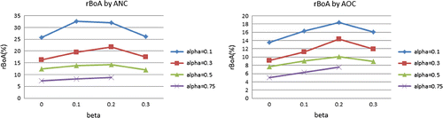
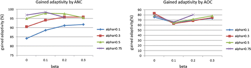
We now investigate the fraction of the maximum benefit of adaptivity captured by the 1-level adaptive policies: (without committing) and (with committing). This ratio takes on values in , and the closer it is to 100%, the greater proportion of the benefit is captured by the 1-level adaptive policies. Due to the existence of the sampling error of our Monte Carlo estimator for and however, the ratio can occasionally exceed 1. Table 3 shows the results for each of the four low-dimensional cases, averaged over the 90 instances for each case. The results of 1-AOC for EMC-LCV are omitted from the table, as the denominator is close to 0. The table shows that 1-ANC has excellent performance, mostly capturing (well) above of the maximum benefit of adaptivity. has a decent performance, capturing of the benefit of adaptivity. Figure 3 shows that the performance of the heuristic is robust over a wide range of values for and .

Table 3. The fraction of the benefit of adaptivity gained by the heuristics for the four low-dimensional cases. Reported numbers correspond to the average and standard deviation over the 90 instances for that case.

Case name	ANC	AOC
vHOHWK-HCV
vHOHWK-LCV
EMC-HCV
EMC-LCV		Omitted

Table 4. Most common scheduling sequence under and corresponding fraction of sample paths in which this sequence is used for and .

Case	Most common sequence	Fraction (1-ANC) (%)	Fraction (1-AOC) (%)
vHOHWK-HCV	(3,2,1)	98.73	66.23
vHOHWK-LCV	(3,2,1)	84.90	60.86
EMC-HCV	(3,2,1)	99.78	18.25
EMC-LCV	(3,2,1)	75.26	57.51

Figure 3. The fraction of the benefit of adaptivity captured by the heuristics for various values of and . Each point represents the average of 24 instances that use that specific value of , and the average of 18 instances for the 1-AOC.

6.3. Insights from the schedules

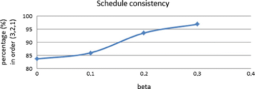
We inspect sample paths of the 1-ANC and 1-AOC schedules, to obtain insights into the order in which patients from various patient classes should be sequenced. Patient classes for the low-dimensional instances are numbered in order of increasing standard deviation, see Table B1 in Appendix B.2. Table 4 shows the frequencies of the most common sequences. The results in the table represent the average over 90 instances per case (see Section 4), and 2000 sample paths per instance. The table shows that the 1-ANC policy typically sequences patients in order of decreasing standard deviation. To a lesser degree, this also holds for 1-AOC. The degree by which sequences adhere to this order increases with , as shown in Figure 4.

Figure 4. Dependence of schedule consistency, i.e. fraction of schedules in the order (3, 2, 1), on .

6.4. Computational efficiency

We investigate the computational efficiency of the 1-level adaptive policies and the optimal adaptive policies. An important factor governing running time is the number of patient classes. We first test the computational efficiency using the 360 low-dimensional problem instances described in Section 6.2. These instances have only three patient classes. Our experiments indicate that the number of patients per class is the main factor determining running time for these instances. We therefore plot the running time against this parameter in Figure 5. Computations were performed using a laptop with an i5-3210M CPU and 8GB RAM. The figure shows that while the 1-level adaptive policies computes solutions nearly instantly, the computation times for the optimal adaptive policy increase rapidly as the number of patients per class grows.

To investigate the scalability of the policies for cases with more patient classes, we perform additional tests for the cases Ophthalmology and Gynaecology (see Table 1). We determine the average computation time for 15 combinations of the parameters (see Section 6.1). The results are summarised in Table 5. The table shows that the computation times for the 1-level adaptive policies are shorter than 1.2 min: short enough for application in practice. However, the computation times for the optimal adaptive policy are quite significant: for the cases with 18 patients over 6 or 9 classes, the computation time even exceeds 24 h. We conclude that the optimal schedules cannot be computed in a reasonable timescale for cases with moderate numbers of patients and patient classes.

Figure 5. The running time of the various adaptive policies for cases with 3 patient classes. Each data point corresponds to the average of 60 instances that share the same number of patients per class.

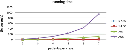
Table 5. Running time of various adaptive policies for high-dimensional problems.

Case	# patients per class	1-ANC	1-AOC	ANC	AOC
2*Ophthalmology	(2,2,2,2,2,2)	0.2 min	0.2 min	5.4 min	57 min
	(3,3,3,3,3,3)	0.4 min	0.2 min	h	h
2*Gynaecology	(1,1,1,1,1,1,1,1,1)	0.1 min	0.2 min	6.6 min	161 min
	(2,2,2,2,2,2,2,2,2)	1.2 min	0.6 min	h	h

6.5. The benefits of adaptive scheduling at Erasmus Medical Center

For the four realistic high-dimensional cases given in Table 1, the optimal adaptive policies ANC and AOC are computationally intractable, as shown in Table 5. However, our efficient 1-level adaptive policies 1-ANC and 1-AOC can be applied to these instances. We use one patient per class for Orthopaedics and Urology, and consider two options for the patients per class for Gynaecology and Ophthalmology. The results are given in Table 6, which reports the estimated relative improvement of 1-AOC and 1-ANC in comparison to StS. For reward parameters, we set , and . The table shows a substantial improvement for the 1-level adaptive policy without committing as well as for the 1-level adaptive policy with committing, be it to a smaller extend. We can clearly identify that the relative improvement decreases in , but no explicit tendency in . It also tends to increase in the average CV. The two percentages in bold face are low because all the mean surgical times of Orthopaedics are relatively long, and overtime cost is relatively high compared with reward. As a consequence, only two to three surgeries are selected by our heuristic during the day, which limits its potential. Interestingly, one of these orthopaedics cases forms the only exception where the improvement over the optimal static scheduling is not statistically significant at the 5% level.

Table 6. The relative improvement of 1-ANC and 1-ANC compared to StS for 4 specialism and various numbers of patient per class, estimated using Monte Carlo.

			1-ANC
Case	Avg. CV	# of patients
2*Ophthalmology	2*0.31	(1,2,1,2,1,2)
		(2,2,2,2,2,2)
2*Gynaecology	2*0.35	(1,1, ...,1)
		(2,2, ...,2)
Orthopedics	0.29	(1,1, ...,1)		%
Urology	0.24	(1,1, ...,1)		%
			1-AOC
Case	Avg. CV	# of patients
2*Ophthalmology	2*0.31	(1,2,1,2,1,2)
		(2,2,2,2,2,2)
2*Gynaecology	2*0.35	(1,1, ...,1)
		(2,2, ...,2)
Orthopedics	0.29	(1,1, ...,1)
Urology	0.24	(1,1, ...,1)

7. Discussion and conclusion

Adaptive scheduling has received considerable attention from the operations research community since the seminal work of Dean, Goemans, and Vondrák (2008), but has so far not been applied to operating room production research, where adaptive scheduling is common practice May et al. (2011). Our work is the first to introduce formal adaptive models and solution methods to the field of operating room scheduling. For the purpose of making the models more realistic and practically applicable to operating room planning, we introduce the concept of committing, thus extending the existing adaptive models to adaptive models with committing. The presented analysis applies the l-level adaptive policies proposed by Ilhan, Iravani, and Daskin (2011) and extensions of these policies to adaptive policies with committing. Our analytical results demonstrate that committing deteriorates performance, while adaptivity enhances performance. Moreover, we show that l-level committing adaptive policies outperform the static policy in expectation. For practical purposes, the concept of adaptive scheduling with committing can be further refined to better match the reality of operating room scheduling. For instance, the level of committing can decrease as the day progresses, and extensions to incorporate arrival of acute patients are of interest.

For practical implementation, l-level adaptive policies require an efficient exact method for the static problem. We develop such an algorithm in the form of a new pseudo-polynomial dynamic programming algorithm that is valid for the broad class of additive distributions, which includes the normal distribution. This algorithm for the static problem therefore is considerably more general than existing approaches, which typically assume normal distributions. The computational analysis demonstrates the efficiency of the dynamic programming algorithm.

The performance analysis on practical problems shows that the 1-level adaptive policy tends to capture most of the gap between the static and the optimal adaptive policy. For instances based on real-life data, the 1-level adaptive policy gives a statistically significant performance benefit of 2 to 15%. The 1-level 1-committing adaptive policy, which may be preferred in practice because it does not make last-minute changes, typically gives significant performance benefits in the order of 2 to .

Now let us turn to the practical implications and derive some practical guidelines from the analysis and results. We observe from our computational experiments that adaptivity brings substantial and significant performance gains over static policies, thus explaining why it is commonly practised in the first place. As shown by Stepaniak, Mannaerts, et al. (2009), Stepaniak et al. (2012) however, the adaptation decisions made by human planners may differ considerably and lead to considerable performance differences. Hence, the proposed models and methods may be of value by enabling consistent performance improvement. The 1-level adaptive algorithms in particular are computationally efficient and provide near optimal solutions.

To use these algorithms in practice, it is required to set an appropriate level of committing, so as to balance inconveniences from adaptivity for the patients with other performance attributes such as risk of cancellation, overtime costs, hospital revenue and employee dissatisfaction from overtime work. Our analysis does not provide optimal levels of committing, these need to be set by management. Analysing these trade-offs can also be viewed as an area for further research. Practical application will also require that the rewards of treating patients are quantified relative to overtime costs. This also requires managerial judgement, as these rewards and costs also include constituents which are not trivially quantified (e.g. health outcomes, and employee dissatisfaction). Future research to learn these parameter values from empirical decisions is called for.

Finally, our results show that, as a rule, adaptive policies tend to sequence long surgeries and surgeries with relatively large standard deviations early. Thus, until decision support for adaptive scheduling is available, these rules of thumb might already guide practical adaptive operating room scheduling.

Additional information

Funding

The First author was supported by the CSC China Scholarship Council.

Notes

No potential conflict of interest was reported by the authors.

Appendix 1

Proofs of theorems

Recall that is defined as the optimal solution to the static problem, with the additional restriction that patients of each class i must be scheduled. In particular, if we consider the constraints(A1)

then define as (1-4+A1(A1) ). Note that this definition is in line with our definition of in Section 3.2.1. Moreover, let .

We first present some results concerning that will be useful in the proofs of Theorems 1–3.

Lemma 1

For any t, , such that , and , it holds that

Proof Denote any feasible solution of as , , . According to the definition of , we can derive that for , and . Moreover, due to .

Let equal excluding element which is 1 for sure, then is also a feasible solution of for any realisation of . Its objective value for is definitely no bigger than the optimal value of . But, taking the expectation, this objective value equals with solution . This proves the lemma.

Lemma 2

For any t, , such that , it holds that

Proof We first note that is a relaxation of for all i and of , so and , . This proves

Next we will prove the reverse inequality. Let , , denote the optimal solution to . The one of the following two must be true:

• if , s.t. , then we can add this constraint to without changing the objective function to obtain . So .

• if for , , then .

This proves the reverse inequality, which completes the proof.

Theorem 1

For any remaining time t, patient vector , committed patient vector , and for , it holds that

and for policies without committing and , it holds that

Proof We will first prove . We have

Here, and throughout this appendix, we let and . (The subscript of the first coordinate c of is omitted to improve legibility.) Here, the first equality follows from Lemma 2 with , and the inequality from Lemma 1 with . The final equality is a specialisation of (9) to . The result follows likewise, by noting that , with the zero vector.

Now, we prove for all by induction on l. We just proved . Assume the inequality holds for . If , we have(A2)

From this, the induction step follows readily. More precisely, if attains the outer maximum in (A2(A2) ), then the result is immediate. On the other hand, if attains the maximum, let attain the inner maximisation and . Then,

where the first inequality follows from induction hypothesis. If , it also holds using their definitions and results of when . This completes the proof by induction. The proof of goes in the same fashion.

Finally, we need to prove that for any and any , with , it holds that . For ease of exposition, we define . We proceed by induction on . For , we have , because are all the available patients since . Now, assume the statement holds for some , and let be any patient vector such that . If , we then have(A3)

because , implying that by induction hypothesis. This completes the inductive argument.

For the proof of , induction starts at , for which the result is immediate because since implies there are no patients. The induction step goes similar to the induction step for the case with committing.

Theorem 2

For any remaining time t, patient vector , committing vector , s.t. , and adaptivity level , it holds that and .

Proof We show that for any , any and with and any and t it holds that . We proceed by induction on when . For , , since only patients are left. Now, assume the statement holds for . For any t, , , such that , and , we have:

where .

Case 1: attains the maximum. In that case, . Case 2: attains the maximum. In that case, let denote the patient class that attains the inner maximum and . We thus obtain

Here, the first inequality is a consequence of Theorem 1. The second inequality is the induction hypothesis, which may be applied because . The final equality in fact corresponds to the definition of , because by assumption, patient class j was optimal for . This completes the induction step. Using this result and definitions of and we can deduce that . The proof of goes likewise.

Theorem 3 (committing deteriorates performance)

Let with and consider committing vectors and . Then, for any time t, patient vector such that , and adaptivity level it holds that

and that:

Proof We first consider the case : let and . We will prove that by induction on l. For , the result follows from , which follows readily from Lemma 1 since by assumption. Now, let the induction hypothesis be that the statement holds for some l. Denote . We have

Case 1: suppose that attains the maximum. Then

so we obtain .

Case 2: Suppose:

Denote . Then

where the first inequality follows from induction hypothesis. This completes the induction step, which completes the proof of the case . The general case where follows by repeatedly applying the case .

The second claim follows from the first claim by noting that Theorem 1 guarantees that and for .

Theorem 4

For any parameter , and state , , with .

Proof According to the definitions in (11(11) ) and (12(12) ), let () be the optimal solution to , it is also a feasible solution to , it is easy to deduce that . On the contrary, with fixed , the second term in is fixed, maximise is equivalent to maximise , and if no feasible solution exist, both objective functions are . Therefore, for any group and .

Theorem 5

For any and , prove(A4)

Proof We will give the proof by induction.

• For , if , by letting , both sides of (A4(A4) ) get value , else both equal to . Therefore the theorem is true for .

• Assume the recursion is correct for and , next we will prove it is also correct for .

  • if , s.t. , , then , denoting its optimal solution as , then . For the right hand side of expression (A4(A4) ), we let ,

    • if , then is a feasible solution of

    • if , then is a feasible solution of

    thus: and vice versa.

  • if is not feasible, i.e. , s.t. , , based on definition (2), we have . For the right-hand side of (A4(A4) ), if there exists a , s.t. .

    • if , and is a feasible solution of , then .

    • if , and is a feasible solution of , then by letting , .

    Then it contradicts to our assumption. So the right-hand side of (A4(A4) ) is also , and the theorem is true.

Appendix 2

Surgical time distributions

Finite parameter compound Poisson distributions

We use a finite-parameter compound Poisson distribution to fit the surgical time. A Poisson random variable with rate will be denoted by .

To construct the finite-parameter class with m parameters, we can freely choose constants as coefficients of a series of Poisson random variables. After these constants are fixed, each distribution in the class will be fully characterised by the rates of Poisson random variables for . If for class i we have , then the surgical time for this class is distributed as follows:

Because , this class of compounding distributions is closed under addition. It will be denoted as , . For our experiments, we will use three parameters ().

Surgical time distributions for the benchmark cases

In this appendix, we give the parameters and for each of the patient classes in each of the cases that are used in our numerical experiments. Two low-dimensional cases were based on mean and variance of surgery distributions from Van Houdenhoven et al. (2007), and two cases were based on data from Erasmus medical centre. Data for these cases are summarised in Table B1. Four high-dimensional cases correspond to the patient classes in four specialisms at Erasmus medical centre. Data are summarised in Table B2.

Table B1. Parameters of surgical times and fitting coefficients for low dimensional instances

	Van Houdenhoven et al. (2007) (vHOHWK)			Erasmus medical center
Groups	Class #	(mean,SD)		Class #	(mean,SD)
4*High CV	1	(80, 65)	(3.838,0, 0.149)	1	(62,18)	(12.371, 0.001, 0.003)
	2	(119, 107)	(3.159,0, 0.477)	2	(97,32)	(17.349, 0.002, 0.168)
	3	(192, 165)	(0.777,0, 1.202)	3	(181,57)	(27.914, 0.004, 0.692)
	Avg. CV=0.86			Avg. CV=0.31
4*Low CV	1	(135, 52)	(8.714,0, 0.024)	1	(187,33)	(34.805, 0.861, 0)
	2	(100, 68)	(5.363,0, 0.111)	2	(215,41)	(35.298, 2.225, 0.081)
	3	(102, 125)	(0.926,0, 0.503)	3	(276,53)	(37.960, 4.942, 0.205)
	Avg. CV=0.76			Avg. CV=0.19

Table B2. Surgical time mean, standard deviation, and fitting parameters obtained for procedures in various categories, from the data of Erasmus medical centre.

Case	(mean,SD)
	(85.31,12.95)	(18.249,0,0)
Ophthalmology	(55.35,17.92)	(10.904,0.001,0.013)
	(110.76,38.85)	(18.670,0.002,0.289)
	(87.31,27.99)	(16.194, 0.002, 0.105)
	(53.82,19.92)	(10.296, 0.001, 0.038 )
	(71.03,24.32)	(13.340, 0.002, 0.071)
	(135.53, 44.85)	(22.249, 0.003, 0.403)
Gynaecology	(150.27,39.74)	(27.033,0.004,0.250)
	(121.81,38.32)	(21.229,0.003,0.260)
	(73.13,29.69)	(12.744,0.002,0.156)
	(87.57,22.67)	(17.231,0.002,0.022)
	(190.14,81.25)	(17.473,0.002,1.712)
	(249,65.65)	(34.694,1.614,0.855)
	(253.04,88.47)	(26.736,0.004,1.988)
	(117.02,64.55)	(10.376,0.001,1.085)
	(49.6, 12.44)	(10.349,0,0)
	(276.25, 52.91)	(37.960,4.942,0.205)
	(187, 32.66)	(34.805,0.861,0)
	(79.47, 17.35)	(16.337,0,0)
	(66.38, 15.69)	( 13.671,0,0)
Urology surgery	(214.75, 40.93)	(35.298,2.225,0.081)
	(181.2, 56.51)	(27.914,0.004,0.692)
	(121.55, 27.55)	(23.751,0.003,0.045)
	(53.27, 10.39)	(11.382,0,0)
	(42.03, 10.02)	(8.911,0,0)
	(96.87, 32.24)	(17.349,0.002,0.168)
	(62.09, 17.94)	(12.371,0.001,0.003)
	(77.93, 21.75)	(15.278,0.002,0.025)
	(143.11, 37.79)	(26.022,0.003,0.215)
	(159.89, 38.72)	(29.422,0.004,0.211)
	(77.15, 56.21)	(5.339,0,0.840)
Orthopedic surgery	(235.58, 88.46)	(22.934,0.003,2.014)
	(258.68, 61.49)	(35.852,2.786,0.627)
	(144.77, 25.16)	(29.369,0,0)
	(144.25, 28.46)	(28.517,0.004,0.026)
	(167.56, 40.01)	(30.727,0.004,0.230)
	(149.14, 26.51)	(30.024,0,0)

Compound Poisson goodness of fit

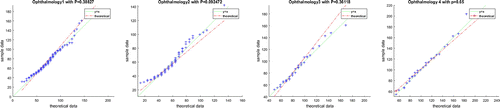
We test the goodness of fit of the three-parameter compound Poisson distribution for fitting the surgery time data obtained from Erasmus medical centre. The data that we fit includes a set-up time of 20 min for cleaning and sterilisation, which is added to each surgical time before distribution estimation.

For our tests, we focus on procedures with the largest number of samples in each of the four specialism. Throughout, we use , and we fit the parameters based on mean and variance of the samples. The goodness of fit of the resulting distributions is analysed by Quantile–Quantile Plot (qq-plot) and a chi-square test. In all the graphs below, the solid line with works as a benchmark to reflect a perfect fit. The dashed line is the quantile values corresponding to the theoretical compound Poisson distribution, and dots are our samples. If two distributions are similar, the points will approximately lie on the green line; if there exists an approximate affine relation, the points are approximately on a straight line. From Figures B1–B4, we observe that the distributions fit the data quite well. A chi-squared goodness of fit test with 9 bins confirms this hypothesis at the significance level .

Figure B1. Gynaecology surgery.

Figure B2. Urology surgery.

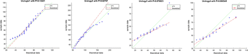
Figure B3. Orthopaedy surgery.

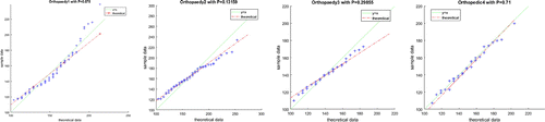
Figure B4. Ophthalmology surgery.

References

- Balseiro, S. R., and D. B. Brown. 2016. Approximations to Stochastic Dynamic Programs via Information Relaxation Duality. Tech. rep., Working Paper. http://faculty.fuqua.duke.edu/\~dbbrown/bio/papers/balseiro\_brown\_approximations\_16.pdf.
- Batun, S., B. T. Denton, T. R. Huschka, and A. J. Schaefer. 2011. “Operating Room Pooling and Parallel Surgery Processing under Uncertainty.” INFORMS Journal on Computing 23 (2): 220–237.
- Bhalgat, A., A. Goel, and S. Khanna. 2011. “Improved Approximation Results for Stochastic Knapsack Problems.” In Proceedings of the Twenty-second Annual ACM-SIAM Symposium on Discrete Algorithms, 1647–1665. SIAM.
- Blado, D., W. Hu, and A. Toriello. 2016. “Semi-infinite Relaxations for the Dynamic Knapsack Problem with Stochastic Item Sizes.” SIAM Journal on Optimization 26 (3): 1625–1648.
- Brauner, N., Y. Crama, A. Grigoriev, and J. van de Klundert. 2005. “A Framework for the Complexity of High-multiplicity Scheduling Problems.” Journal of Combinatorial Optimization 9 (3): 313–323.
- Cardoen, B., E. Demeulemeester, and J. Beliën. 2010. “Operating Room Planning and Scheduling: A Literature Review.” European Journal of Operational Research 201 (3): 921–932.
- Cayirli, T., and E. Veral. 2003. “Outpatient Scheduling in Health Care: A Review of Literature.” Production and Operations Management 12 (4): 519–549.
- Chen, K., and S. M. Ross. 2014. “An Adaptive Stochastic Knapsack Problem.” European Journal of Operational Research 239 (3): 625–635.
- Dean, B. C., M. X. Goemans, and J. Vondrák. 2008. “Approximating the Stochastic Knapsack Problem: The Benefit of Adaptivity.” Mathematics of Operations Research 33 (4): 945–964.
- Dellaert, N., E. Cayiroglu, and J. Jeunet. 2016. “Assessing and Controlling the Impact of Hospital Capacity Planning on the Waiting Time.” International Journal of Production Research 54 (8): 2203–2214.
- Denton, B., J. Viapiano, and A. Vogl. 2007. “Optimization of Surgery Sequencing and Scheduling Decisions under Uncertainty.” Health Care Management Science 10 (1): 13–24.
- Dexter, F., R. H. Epstein, R. D. Traub, and Y. Xiao. 2004. “Making Management Decisions on the Day of Surgery Based on Operating Room Efficiency and Patient Waiting Times.” Anesthesiology 101 (6): 1444–1453.
- Dexter, F., A. Macario, and R. D. Traub. 1999. “Which Algorithm for Scheduling Add-on Elective Cases Maximizes Operating Room Utilization? Use of Bin Packing Algorithms and Fuzzy Constraints in Operating Room Management.” Anesthesiology 91 (5): 1491–1500.
- Dexter, F., A. Macario, R. D. Traub, M. Hopwood, and D. A. Lubarsky. 1999. “An Operating Room Scheduling Strategy to Maximize the Use of Operating Room Block Time: Computer Simulation of Patient Scheduling and Survey of Patients’ Preferences for Surgical Waiting Time.” Anesthesia & Analgesia 89 (1): 7–20.
- Dexter, F., A. Willemsen-Dunlap, and J. D. Lee. 2007. “Operating Room Managerial Decision-making on the Day of Surgery with and without Computer Recommendations and Status Displays.” Anesthesia & Analgesia 105 (2): 419–429.
- Erdogan, S. A., B. T. Denton, J. Cochran, L. Cox, P. Keskinocak, J. Kharoufeh, and J. Smith. 2011. Surgery Planning and Scheduling. Wiley Encyclopedia of Operations Research and Management Science. http://ca.wiley.com/WileyCDA/Section/id-380199.html.
- Garey, M. R., and D. S. Johnson. 1979. Computers and Intractability: A Guide to the Theory of NP-completeness. San Francisco, CA: WH Freeman & Co.
- Gupta, D. 2007. “Surgical Suites’ Operations Management.” Production and Operations Management 16 (6): 689–700.
- Gupta, D., and B. Denton. 2008. “Appointment Scheduling in Health Care: Challenges and Opportunities.” IIE Transactions 40 (9): 800–819.
- Hochbaum, D. S., and R. Shamir. 1990. “Minimizing the Number of Tardy Job Units under Release Time Constraints.” Discrete Applied Mathematics 28 (1): 45–57.
- Hochbaum, D. S., and R. Shamir. 1991. “Strongly Polynomial Algorithms for the High Multiplicity Scheduling Problem.” Operations Research 39 (4): 648–653.
- Ilhan, T., S. M. Iravani, and M. S. Daskin. 2011. “Technical Note -- The Adaptive Knapsack Problem with Stochastic Rewards.” Operations research 59 (1): 242–248.
- Jebali, A., and A. Diabat. 2015. “A Stochastic Model for Operating Room Planning under Capacity Constraints.” International Journal of Production Research 53 (24): 7252–7270.
- Kleywegt, A. J., A. Shapiro, and T. Homem-de Mello. 2002. “The Sample Average Approximation Method for Stochastic Discrete Optimization.” SIAM Journal on Optimization 12 (2): 479–502.
- Levin, A., and A. Vainer. 2013. “The Benefit of Adaptivity in the Stochastic Knapsack Problem with Dependence on the State of Nature.” Discrete Optimization 10 (2): 147–154.
- May, J. H., W. E. Spangler, D. P. Strum, and L. G. Vargas. 2011. “The Surgical Scheduling Problem: Current Research and Future Opportunities.” Production and Operations Management 20 (3): 392–405.
- Merzifonluoğlu, Y., J. Geunes, and H. E. Romeijn. 2012. “The Static Stochastic Knapsack Problem with Normally Distributed Item Sizes.” Mathematical Programming 134 (2): 459–489.
- van Oostrum, J. M., M. Van Houdenhoven, J. L. Hurink, E. W. Hans, G. Wullink, and G. Kazemier. 2008. “A Master Surgical Scheduling Approach for Cyclic Scheduling in Operating Room Departments.” OR Spectrum 30 (2): 355–374.
- Shylo, O. V., O. A. Prokopyev, and A. J. Schaefer. 2012. “Stochastic Operating Room Scheduling for High-volume Specialties under Block Booking.” INFORMS Journal on Computing 25 (4): 682–692.
- Stepaniak, P., C. Heij, G. Mannaerts, M. de Quelerij, and G. De Vries. 2009. “Modeling Procedure and Surgical Times for Current Procedural Terminology-anesthesia-surgeon Combinations and Evaluation in Terms of Case-duration Prediction and Operating Room Efficiency: A Multicenter Study.” Anesthesia & Analgesia 109 (4): 1232–1245.
- Stepaniak, P. S., G. H. H. Mannaerts, M. de Quelerij, and G. de Vries. 2009. “The Effect of the Operating Room Coordinator’s Risk Appreciation on Operating Room Efficiency.” Anesthesia & Analgesia 108 (4): 1249–1256.
- Stepaniak, P., R. van der Velden, J. van de Klundert, and A. Wagelmans. 2012. “Human and Artificial Scheduling System for Operating Rooms.” In Handbook of Healthcare System Scheduling, 155–175. Springer.
- Tang, J., and Y. Wang. 2015. “An Adjustable Robust Optimisation Method for Elective and Emergency Surgery Capacity Allocation with Demand Uncertainty.” International Journal of Production Research 53 (24): 7317–7328.
- Van Essen, J. T., J. M. Bosch, E. W. Hans, M. van Houdenhoven, and J. L. Hurink. 2014. “Reducing the Number of Required Beds by Rearranging the OR-schedule.” OR spectrum 36 (3): 585–605.
- Van Houdenhoven, M., J. M. van Oostrum, E. W. Hans, G. Wullink, and G. Kazemier. 2007. “Improving Operating Room Efficiency by Applying Bin-packing and Portfolio Techniques to Surgical Case Scheduling.” Anesthesia & Analgesia 105 (3): 707–714.
- Vermeulen, I. B., S. M. Bohte, S. G. Elkhuizen, H. Lameris, P. J. Bakker, and H. La Poutré. 2009. “Adaptive Resource Allocation for Efficient Patient Scheduling.” Artificial Intelligence in Medicine 46 (1): 67–80.
- Vissers, J. M., J. Bertrand, and G. De Vries. 2001. “A Framework for Production Control in Health Care Organizations.” Production Planning & Control 12 (6): 591–604.
- Wang, Y., J. Tang, and R. Y. Fung. 2014. “A Column-generation-based Heuristic Algorithm for Solving Operating Theater Planning Problem under Stochastic Demand and Surgery Cancellation Risk.” International Journal of Production Economics 158: 28–36.
- Xiao, G., W. van Jaarsveld, M. Dong, and J. van de Klundert. 2016. “Stochastic Programming Analysis and Solutions to Schedule Overcrowded Operating Rooms in China.” Computers & Operations Research 74: 78–91.
- Zhang, Z., X. Xie, and N. Geng. 2014. “Dynamic Surgery Assignment of Multiple Operating Rooms with Planned Surgeon Arrival Times.” IEEE Transactions on Automation Science and Engineering 11 (3): 680–691.
- Zhou, J., F. Dexter, A. Macario, and D. A. Lubarsky. 1999. “Relying Solely on Historical Surgical Times to Estimate Accurately Future Surgical Times is Unlikely to Reduce the Average Length of Time Cases Finish Late.” Journal of Clinical Anesthesia 11 (7): 601–605.