Measuring productive performance using binary and ordinal output variables: the case of the Swedish fire and rescue services

Abstract

Fire protection is an example of a complex production process. This study measures efficiency by constructing binary and ordinal output variables from information on residential fires in Sweden about how a fire spreads from when the fire and rescue brigade arrives to when a fire is suppressed. The motivations behind this study are that there are only a few studies trying to estimate production efficiency for fire and rescue services, that data on a more detailed level is interesting for some public services, and there is a need to be able to measure efficiency differences even if only a binary or ordinal output variable is available. Using a logit random parameter model, the random effects are interpreted as efficiency differences. The conclusions are that fire and rescue services with a more flexible fire organisation with first response persons, working in collaboration with other municipalities and with larger populations are more efficient.

Keywords:

• qualitative output
• efficiency
• productivity
• logit parameter model
• fire departments

1. Introduction

Measuring efficiency and productivity are quite straightforward for most private goods-producing firms. If the output is relatively homogenous, the outputs can be directly compared to inputs for different decisionmaking units. The less homogenous the output, the more difficult the efficiency measuring becomes. For public agencies, the output is often more heterogeneous. One reason is that most often service is produced and the quality of service varies depending on the how the ‘consumer’ perceives it. Many public agencies also have a complicated structure when it comes to the relation between input and output, and there is a choice which output measure to; intermediate output, direct output, final output, consequences or welfare aspects (Bradford, Malt, and Oat 1969; Balaguer-Coll, Prior, and Tortosa-Ausina 2013).

Fire protection is one example of such a complex production process. Fire and rescue services both try to prevent fires from happening and when they happen, to suppress them as effectively as possible. Considering the suppressing activity, the outcome can be measured as an intermediate output using (e.g., manning level and response time), as a direct output (e.g., number of fires suppressed), as a final output (e.g., saved property and lives) and as a welfare measure (Jaldell 2002).

Yet another problem may be that the outcome cannot always be measured continuously. This is especially true when output is measured on a detailed level. Did the police get the thief, or not? What grade did the pupil get? Did the fire and rescue services suppress the fire, or not? In this study, we use data on each individual alarm to fire and rescue services and, therefore, outcome is measured on a very detailed level. One solution to this problem can be to use a more aggregate level. However, the output in that case only becomes fractions (e.g. lives saved per alarm). Aggregation also leads to information being lost, and for fire and rescue services this includes crucial information about an important factor: the response time.

In addition to the problem of measuring the output of public agency, fires are unpredictable. A fire is a continuous process and the task of the fire brigade is to change this process. The output should be measured as the difference between what could have happened, the potential damage, and what actually happened. No matter how many resources the fire service uses on prevention activities, such as inspections and information, fires and other accidents will happen. Uncontrollable factors also influence fire suppression. If there is a fire, the fire service arrives, and the result of the turn-out depends not only on their own activity (the response time, the number and skills of the firefighter), but also on environmental factors (the weather, building conditions, etc.). The outcome of the firefighter's work can also differ among buildings with the same response time, even though the same number of firefighters and trucks are used. Estimating the productivity and efficiency of each fire and rescue service should, therefore, consider this randomness. This paper takes these problems into account by using a logistic random parameter model to estimate efficiency differences between different fire and rescue services, where the individual random effects are interpreted as efficiency differences.

Overall, there are few studies on efficiency or other performance measures of fire and rescue services (Green and Kolesar 2004). The structure of fire prevention and suppression activities with three different levels of outputs may be an explanation for the diversity in output measures (see Duncombe and Brudney 1995; Jaldell 2002; Weinholt 2015). Data envelopment analyses (or similar non-parametric techniques) have been performed for fire services in Sweden (Jaldell 2002), Spain (Sánchez 2006), in the United Kingdom (Athanassaopoulos 1998, in Florida, United States (Choi 2005), in Taiwan (Lan, Chuang, and Chen 2009) and in Estonia (Reiljan, Puolokainen, and Ülper 2015). In a comparison of eight countries’ fire protection, Sweden was one of the countries and Sweden needed, according to the study, to increase its scale of operations and adjust its technique (Peng et al. 2014).

While none of the above-mentioned studies looked at the third (final) output step, a few have done so. Two used a continuous measure for wildfire spread (Holmes and Calkin 2013; Katuwal, Calkin, and Hand 2016), but the paper most similar to this study measured suppression efficiency using an ordinal probit model (Jaldell 2005). A three-level output variable was constructed from data on the spread of fires in detached houses in Sweden in a similar way as is done here. The output was compared to the inputs response time, own firefighters, firefighters from other fire services, full-/or part-time firefighters and life-saving activities. Another paper using an ordinal output variable is Griffiths, Zhang, and Zhao (2014) that used a Bayesian approach to estimate the efficiency for individual health production in Australia.

There are two purposes of this study. The first purpose is to show how efficiency can be measured using qualitative output variables. There have been incredibly many efficiency studies using continuous output measures, but as discussed hardly anyone using binary or ordinal output measures. Data on a more detailed level are interesting for many public services and there is a need to be able to measure efficiency differences even if only a binary or ordinal output variable is available. This study uses models with parametric functions. The second purpose is to measure efficiency for Swedish fire and rescue services and understand why these may differ. As shown above there have been only a few studies on the performance of fire and rescue services worldwide using production functions and efficiency (Green and Kolesar 2004).

2. Data

The fire and rescue services in Sweden have two tasks. The first is to prevent fires from happening and the second is to suppress them, if they develop, as quickly and efficiently as possible. The municipalities are fully responsible for organizing the fire and rescue services in Sweden. They do it either on their own or in collaboration with other municipalities. There are 290 municipalities and about 150 fire and rescue services. There are two types of firefighters: full- and part-time. Full-time firefighters are employed by the fire and rescue services and are prepared at the fire station 24 hours a day. Normally they should be on the way in 90 seconds after an alarm. Part-time firefighters have other jobs and must get to the fire station after an alarm. They are on their way after 5–6 minutes. To further decrease the response time, more flexible solutions using so-called first response persons have been tested. A first response person is a single fire fighter who may be situated in places other than the fire station or be on the way in less than 90 seconds. The fire and rescue service arrives to not only fires, but also traffic accidents, drownings, storm accidents, flooding, etc. However, this study concentrates on residential fires.

Data were gathered from the Swedish fire and rescue services’ incident reports from a five-year period 2009–2013. In total there were 29,813 incidents reports covering residential fires from these years. An incident report was written for each incident and transferred by each fire and rescue service to The Swedish Civil Contingencies Agency (MSB) that collects all incidents reports in Sweden. The transferring to the central agency is voluntary, but in practice, all but a couple of small fire and rescue services (only 0.2% of the population) transfer the incident reports. The incident report follows a national standard and MSB provides guidelines on how to fill out the report, but there may be local variations.

Unfortunately, there is no information about lost property value in the incident reports. One possibility could be to use fatalities. However, since each year about 75 persons are reported dead by the fire and rescue services, there is not enough data for comparing different fire and rescue services. Instead, qualitative output variables were constructed from information in the incident reports about how the fire had spread to the point when the fire and rescue service arrived, and from of the final spread of the fire. The output variables measure the risk of fire spreading after the fire service arrived. Table 1 shows how the different outcomes are used to construct the binary and ordinal variables.

Table 1. Condition of fire upon arrival and extent of spread before being extinguished.

			Final spread
			1	2	3	4	5
			Starting article	Starting room	Starting fire-cell	Starting building	Other buildings	Unknown	Binary variable	Ordinal variable
Condition upon arrival:		No. per year	813	797	250	542	43	4	Defined as worse spread, share	Defined as worst spread, share
1	Fire in the starting article	1081	υ11	υ12	υ13	υ14	υ15		0.090	0.010
2	Fire in the starting room	907		υ22	υ23	υ24	υ25		0.156	0.008
3	Fire in several rooms (same fire-cell)	387			υ33	υ34	υ35		0.035	0.035
4	Fire in several fire-cells	69				υ44	υ45		0.168	0.168
	Binary variable
	Defined as worse spread, share		0.000	0.000	0.159	0.335	1.000		0.108	0.090
	Ordinal variable
	Defined as worst spread, share		0.000	0.000	0.000	0.000	1.000			0.018
	Unknown, already extinguished, only smoke	3217

For a given condition upon arrival, more spread is worse. Looking at each row it is obvious that having an initial condition of fire in the starting article, it is better to extinguish it in the starting article, rather than letting the fire spread to the starting room and so on. A starting article may be a stove, a TV, a bed, etc. For fires starting in the fire article, this means that υ11 ≻ υ12 ≻ υ13 ≻ υ14 ≻ υ15.¹ For all rows, it is better to suppress a fire the less it spreads. To make the analysis as simple as possible, a binary measure of performance was first sought. Consulting fire expertise, the choice was made to consider υ13, υ14, υ15, υ24, υ25 and υ45 as worse outcomes and the rest as better outcomes. The worse outcomes are coded one and the better outcomes are coded zero. Out of the 29,813 residential fires in the incident reports, 12,238 could be classified as better or worse outcomes. The rest were noted as already extinguished or only smoke when the fire and rescue service arrived, or they were the condition upon arrival and/or final spread was unknown. In total, 11% of these were classified as worse outcomes for the binary variable.² An ordinal measure of performance on a three-stage scale was also constructed, where the worse outcome in the binary case was divided into two classes. The worst class being those fires that have spread to other buildings. For the ordinal variable, the classes were coded from 0 to 2 from best to worst cases.

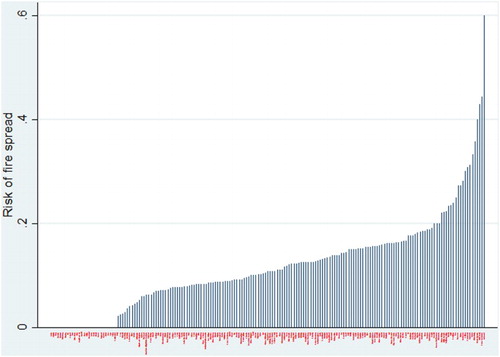
There were differences between the fire and rescue services when it comes to spread of fires as defined here. Figure 1 shows these differences by showing the risk of spread per turn-out for each fire and rescue service for the binary output variable. There were 158 fire and rescue services that had at least one residential fire that spread.³

Figure 1. Distribution of risk of fire spread for the binary variable.

The outcome of the fire also depends on other factors. The tested variables from the incident reports included the response time, fire protection devices such as smoke detectors and portable fire extinguishers, starting room of fire and starting reason of fire. Unfortunately, there is no direct way of reporting first response persons, but a variable was constructed for this defined as when a single firefighter arrives at least two minutes before the other firefighters. Aspects such as the weather, building materials and construction also influence how the fire develops. However, due to the lack of information, these cannot be used. The reason for including response time is that a longer response time may lead to the fire being larger and, therefore, harder to suppress for the fire and rescue service when arriving at the fire.

3. Model

In this study, logit random parameters models for binary and ordinal output variables were used (see e.g. Greene 2008).⁴ The formulation here follows Rabe-Hesketh and Skrondal (2008). Estimation of the models was conducted using Stata 14. The analysis of efficiency was conducted in three steps. In the first step, we estimated the logit random parameters logit models. The models were estimated using different independent variables. The main independent variable was response time, but variables for fire protection and more information about where the fire started and reason for the fire were also tested. The two levels used were responses, and fire and rescue services. In the second step, the estimated fire and rescue service-specific random intercept was used as a relative efficiency measure. Finally, in the third step, the efficiency was compared to specific attributes for the fire and rescue services, such as number of firefighters, whether full- or part-time firefighters were used and the size of the fire and rescue service.

The binary logit model is described in equation 1 using one independent variable, the natural logarithm of the response time in seconds, ln TIME, where i are turn-outs. In Equation (2), the model is reformulated as a linear predictor with a fire and rescue service-specific random intercept ζ_j added. In Equation (2), ζ_j is normally distributed and independent across fire and rescue services.

(1) $E\left(Y\right)=Prob(y_i=1)=\frac{e^{\alpha +{\beta }_t\ast \ln TIM{E}_i}}{1+e^{\alpha +{\beta }_t\ast \ln TIM{E}_i}},$(1) (2) $logit\left\{Prob(Y=1)|\ln TIM{E}_i,{\zeta }_j\right\}=\alpha +{\beta }_t\ast \ln TIM{E}_{ij}+{\zeta }_j,\text{where }{\zeta }_j|\ln TIM{E}_i\sim N(0,\varphi ).$(2)

Other functional forms for response time could have been chosen, but the chosen functional form fits the data well (cf. Jaldell 2017, for fatalities.). The results are presented as coefficients. The marginal effects, i.e. how much the spread of fire changes when the inputs change marginally, are more interesting for continuous variables and, therefore, presented for the response time varible. The marginal effect per minute is calculated as $\mathrm{\partial }E\left(Y\right)/\mathrm{\partial }TIME=60\times (e^{\alpha +\beta \ast lnTIME}/$ $(1+e^{\alpha +\beta \ast lnTIME}{)}^2)/TIME$ and evaluated at median response time.

Six different models are estimated, three using the binary output variable and three using the ordinal output variable. Considering the binary output variable, model B1 is a fixed effect only model with variables for response time,2 fire suppression devices, 17 fire reasons and 17 starting rooms. The purpose is to find out which fire suppression devices, fire reasons and starting rooms that have a statistical significant effect on the spread of the fires. A fire could be harder or easier to suppress depending on which room it is in. It is also possible that different reasons for the fire could affect the ease of suppressing the fire. Model B2 is a random parameter model only including response time as independent variable, thus modelled according to equation 2. Model B3 is a random parameter model also including the statistical significant variables from model B1. Models O1–O3 are parallel to the binary output models, but instead use the ordinal output as dependent variable. The model used is the ordinal logit model for our three-level output variable.⁵

One standard procedure for efficiency estimating is to use stochastic frontier models for estimating differences between firms in an industry or between decisions units in a certain part of the public sector (Kumbhakar and Lovell 2003). The basic stochastic frontier model for panel data is:(3) $y_{it}=\alpha +x_{it}^{\mathrm{\prime }}\beta +{\nu }_{it}-u_{i,}i=1,\dots ,N,t=1,\dots ,T.$(3) There are i firms or decision units observed for t time periods. The dependent variable y_it is the output of the firms and x_it are the vector of inputs of the firms. α is an intercept, β is a vector of coefficients and ν_it is an i.i.d. error term with zero mean and finite variance. u_i, is an indication of time-invariant technical inefficiency,⁶ where u_i≥ 0. If we define α_i = α-u_i, we get the standard panel data model:(4) $y_{it}={\alpha }_i+x_{it}^{\mathrm{\prime }}\beta +{\nu }_{it}.$(4) In our study, we have data in two dimensions, per decision unit and per turn-out. This means that the data is parallel to an unbalanced panel data model, where the t's are the different turn-outs for each fire and rescue service. Comparing Equations (2)–(4) we can, therefore, let the random intercept ζ_j indicate technical inefficiency for each fire and rescue service. The word ‘indicate’ is used since we have not studied the statistical properties of the estimation of ζ_j and its relation to technical inefficiency, u_i. They are probably not straightforward, since that is not true even for the basic stochastic frontier model (Kim and Schmidt 2000). That is one reason for not recalculating our efficiency estimate into a scale from 0 to 1. Another reason is that it is hard using binary and ordinal output variables to interpret such an efficiency measure. It is not obvious what say 80% efficiency means having binary and ordinal output variables. This is contrary to having a continuous output variable where 80% efficiency means that production could be increased by 25% without using more inputs. Since the efficiency indicator in this study is not on a scale from 0 to 1, but goes from minus to plus numbers we have assumed a normal distribution for the random effect, not another distribution such as gamma distribution which is common for a stochastic frontier analysis.

4. Results

4.1. Models B1–B3 and O1–O3

The coefficients for response time were positive for all models, which means that a longer response time results in a fire that is harder to suppress (Table 2). The coefficients can be recalculated into marginal effects, which show how much a changed response time affects the outcome. The marginal effect for the binary output models from a change in the response time by one minute is around 0.005. Since the average spread of fire is around 0.01 five percent fewer fires will lead to worse outcomes if the response time is decreased by one minute on average.

Table 2. Coefficients for estimated models.

	Model B1	Model B2	Model B3	Model O1	Model O2	Model O3
	Binary	Binary	Binary	Ordinal	Ordinal	Ordinal
	Fixed effects All	Random effects	Random effects Some	Fixed effects All	Random effects	Random effects Some
Response time (ln), seconds
Coefficient	0.429*** (0.0619)	0.454*** (0.0586)	0.449*** (0.0618)	0.442*** (0.0617)	0.464*** (0.0586)	0.462*** (0.0616)
Marginal effect per min
Level 0 → 1	0.0044***	0.0051***	0.0048***
→ Level 0				−0.0045***	−0.0053***	−0.0050***
→ Level 1				0.0043***	0.0043***	0.0040***
→ Level 2				0.0009***	0.0009***	0.0009***
Fire suppression devices:
Smoke detector	−0.00992 (0.0803)			−0.00357 (0.0802)
Fire extinguisher portable	−0.136 (0.0838)			−0.131 (0.0835)
Fire reason
Deliberately	0.0195 (0.143)			−0.00973 (0.143)
Other	−0.0216 (0.150)			−0.0303 (0.149)
Children playing with fire	0.561* (0.333)			0.522 (0.331)
Flash of lightning	−0.132 (0.259)			−0.182 (0.258)
Explosion	0.0757 (0.672)			0.212 (0.670)
Fire works	−0.0873 (0.403)			−0.146 (0.402)
Stove	−0.185 (0.200)			−0.186 (0.200)
Sparkles	0.0801 (0.214)			0.119 (0.213)
Hot works	−0.108 (0.317)			−0.105 (0.317)
Candles	−0.721** (0.280)		−0.699*** (0.263)	−0.724*** (0.280)		−0.692*** (0.263)
Unknown	0.230** (0.117)		0.330*** (0.0685)	0.236** (0.117)		0.350*** (0.0683)
Smoking	−0.693*** (0.232)		−0.556*** (0.211)	−0.715*** (0.232)		−0.562*** (0.211)
Autoignition	−0.266 (0.320)			−0.293 (0.319)
Chimney fire	−1.947*** (0.293)		−2.088*** (0.193)	−1.957*** (0.293)		−2.092*** (0.193)
Technical failure	Base		Base	Base		Base
Heat transfer	0.445*** (0.142)		0.439*** (0.106)	0.396*** (0.142)		0.404*** (0.105)
Reigniting	−0.0266 (0.278)			−0.0770 (0.277)
Starting room
Bathroom	0.107 (0.365)			0.0874 (0.365)
Utility room	Base		Base	Base		Base
Hallway	−0.321 (0.314)			−0.335 (0.314)
Other/unknown	0.310 (0.235)			0.316 (0.235)
Boiler room	−0.191 (0.289)			−0.212 (0.289)
Chimney	−0.139 (0.313)			−0.151 (0.313)
Garbage room	−0.352 (0.285)			−0.365 (0.285)
Bedroom	−0.230 (0.268)			−0.242 (0.268)
Stairwell	0.449 (0.535)			0.470 (0.534)
Outdoor	1.329*** (0.238)		1.330*** (0.0815)	1.369*** (0.238)		1.374*** (0.0811)
Living room	−0.123 (0.257)			−0.143 (0.257)
Attic	0.704*** (0.268)		0.671*** (0.146)	0.656** (0.267)		0.626*** (0.145)
Sauna	0.409 (0.327)			0.441 (0.326)
Garage	1.640*** (0.270)		1.588*** (0.152)	1.622*** (0.269)		1.573*** (0.148)
Basement	−0.354 (0.282)			−0.364 (0.281)
Kitchen	−0.205 (0.251)			−0.223 (0.251)
Washing room	−1.092*** (0.396)		−1.095*** (0.325)	−1.106*** (0.395)		−1.097*** (0.325)
Intercept	−4.923*** (0.459)	−4.973*** (0.380)	−5.079*** (0.394)
Cut 1				4.987*** (0.458)	5.035*** (0.380)	5.167*** (0.393)
Cut2				7.003*** (0.464)	6.968*** (0.386)	7.191*** (0.400)
Variance, random intercept		0.1110***	0.0741***		0.1110***	0.0744***
Fire and rescue service		(0.0359)	(0.0267)		(0.0359)	(0.0265)
No. of observations	12220	12220	12220		12220	12220
No. of groups		183	183		183	183
Log likelihood	−3705.9	−4124.4	−3720.1		−4707.4	−4293.3
AIC	7483.7	8254.9	7464.2		9422.7	8612.6
LR test vs logit model, p-value		0.000	0.000		0.000	0.000

Note: Standard errors in parentheses.

*p < .1.

**p < .05.

***p < .01.

In model B3 the variables statistical significant at the 5% level in model B1 are used. Considering reasons for the fire, fires starting by candle lights or smoking are found to be easier to suppress, while those with unknown reason and from heat transfer are harder to suppress. Chimney fires are easiest to stop from spreading. Considering starting room, fires starting outdoors, in the garage or in the attic are harder to suppress. Fires starting in a washing room are easiest to suppress. These reasons and the starting rooms reduced the marginal effect of the response time only slightly. In both models B2 and B3, the random effect for the random intercept of each fire and rescue service was statistically significant. The random effect models were, therefore, preferred to fixed effect models. Neither smoke detectors nor portable fire extinguishers were statistically significant in model B1; meaning that they had no effect on the spread of the final spread of the fire taking fire reasons and starting rooms into account.

Considering the ordinal output models, there are three different marginal effects calculated for each model. If the response time is increased by one minute, the risk of a spread to a worse outcome will increase by about 0.004 and the risk to the worst outcome will increase by 0.001. Since the 0.090% of the outcomes are worse and 0.018, the increase in relative risk is about 5% for both. The statistical significant factors for fire reason and starting room and their effects are the same as for the binary models.

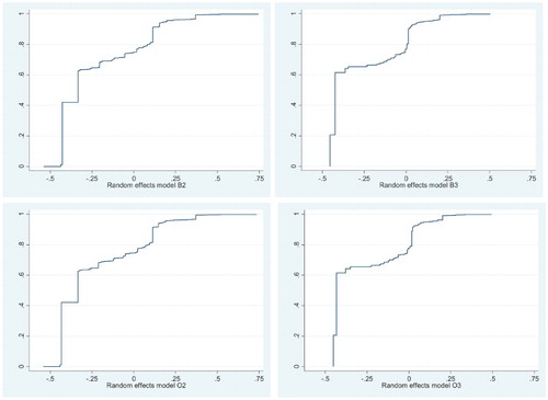
The predicted outcome for using both the response time and the random effect (fire and rescue service specific) from model B2 is shown in Figure 2. The slope of the curve shows that the shorter the response time, the less risk of spread. The random effects are the vertical differences between the diamonds and the curve. However, Figure 2 also shows that the differences between the fire and rescue services are large, implying substantial efficiency differences. Figure 3 shows the cumulative distribution of the random effects from the most efficient (most negative random effect) to the least efficient unit (most positive random effect) from model B3. The cumulative distributions use population weights. The shape of the curve implies that more populated municipalities are more efficient, even more for the models including fire reasons and starting room. Figure 3 also reveals that the shapes of the curves are similar for models B2 and O2, and B3 and O3. This implies that using an ordinal output variable does not affect the estimation of the fire and rescue service random effects and, therefore, does not imply different efficiency patterns.

Figure 2. Predicted values from Model B2.

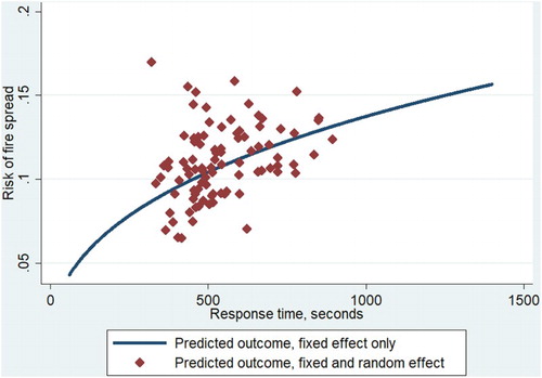
Figure 3. Random effects from Models B2, B3, O2 and O3.

4.2. Analysing the random effects

In this study, we imply that the random effects can be interpreted in efficiency terms. Could there be any organisational differences that could explain the variations in efficiency? One thing could be the size of the fire and rescue service. The hypothesis is that a larger service in a more populated area is more efficient, since more competent personnel could be employed both in the fire crew, but also in management. A larger service could also have better training opportunities and facilities. A fire service in a populated area also has more fires to turn-out to and therefore more experience.

In Table 3, the random effects from models B2, B3, O2 and O3 are regressed on some fire and rescue specific variables.⁷ Number of firefighters, full- or part-time firefighters, association or not population in the area and fires per inhabitant served by the fire and rescue service are all variables that could reflect more competent, and thus more efficient, fire and rescue services. Another interesting variable is the use of first response persons, which should reflect a more flexible service, with a higher efficiency.

Table 3. Explaining random effects with regression analyses.

Model and independent variables	From Model B2	From Model B3	From Model O2	From Model O3
Intercept	0.0735*** (0.0110)	0.151*** (0.00859)	0.0719*** (0.0111)	0.149*** (0.00871)
First response persons	−0.0519*** (0.0105)	−0.0512*** (0.00820)	−0.0516*** (0.0106)	−0.0515*** (0.00830)
No. of firefighters (<16)	−0.000209 (0.000732)	−0.00385*** (0.000570)	−0.000253 (0.000734)	−0.00398*** (0.000577)
Proportion full-time to part-time	0.0965*** (0.0165)	−0.00549 (0.0128)	0.101*** (0.0165)	0.00182 (0.0130)
Only full-time	−0.0846*** (0.0111)	−0.0805*** (0.00865)	−0.0887*** (0.0112)	−0.0874*** (0.00876)
Only part-time	−0.0240** (0.0106)	−0.0301*** (0.00828)	−0.0238** (0.0107)	−0.0286*** (0.00839)
Association	−0.0284*** (0.00593)	−0.0238*** (0.00462)	−0.0270*** (0.00595)	−0.0191*** (0.00468)
Population	−0.000000488*** (1.19e–08)	−0.000000492*** (9.29e–09)	−0.000000493*** (1.20e–08)	−0.000000498*** (9.41e–09)
Number of fires per inhabitant (with output defined as better or worse according to Table 1)	−3.023*** (0.216)	−4.109*** (0.168)	−3.107*** (0.216)	−4.266*** (0.170)
No. of observations	8055	8055	8055	8055
R^2	0.241	0.407	0.244	0.406

Note: Standard errors in parentheses.

*p < .1.

**p < .05.

***p < .01.

The coefficients in Table 3 are negative if the variable results in better performance.⁸ Most variables resulted in a higher efficiency and were statistically significant at the five percent level, except number of firefighters in models B2 and O2, and proportion of full-time to part-time fire fighters in models B3 and O3. Otherwise, using first response persons, only full-time firefighters or only part-time firefighters resulted in fewer fires being spread on average for the fire and rescue service. The coefficient for a mix of full- and part-time firefighters is positive, but the more negative coefficient for full-time fire fighters indicates that they are more efficient than part-time fire fighters. The table also shows that fire and rescue services covering more than one municipality (association), fire and rescue services with a higher population and having more fires per capita are more efficient. The differences between models B2 and B3, and models O2 and O3, were small. More firefighters lead to higher efficiency when correcting for more information about how difficult a fire is to suppress.

An organisational effect is also seen here. Fire and rescue services that use first response persons more, and use more firefighters are more efficient when it comes to suppressing fires.

5. Discussion and conclusion

This study has shown a way of drawing conclusions about performance and efficiency using binary or ordinal output variables. The study should be seen as an empirical example of how an efficiency study could be done using a logit model with random effects influenced by the production frontier literature.

However, since this is a novel empirical study there are some uncertainties. For example, the distance to the frontier is not directly comparable to an analysis using a continuous measure. The econometrical theoretical foundation of the efficiency numbers presented here are unknown. The theoretical connection between the efficiency and the choice of econometric specification is also unknown. At this phase, the performance indicators have not been recalculated into traditional efficiency number. Efficiency numbers in the production frontier literature are typically given on a 0–1 scale, where the index shows degree of efficiency.

Future research could explore both of these questions. However, this study can be seen as a possible step forward for estimating efficiency when a continuous output measure is not possible to find. This may be especially interesting in the public sector where such outputs are relevant including the educational sector (attend university or not), health sector (being cured or not), police sector (get the criminal or not) and social sector (continue getting social allowances or not). Making it possible to use a binary or ordinal output measure also makes it possible to measure performance of units on smaller scale so that aggregation into larger units will not be necessary. The aggregation may lead to having to measure on aggregated units where the most important decisions affecting performance are not taken.

Acknowledgement

The funding body had no role in study design, in the collection, analysis and interpretation of data, in the writing of the report, or in the decision to submit the article for publication.

Disclosure statement

No potential conflict of interest was reported by the author.

Additional information

Funding

This work was supported by the Swedish Civil Contingencies Agency (grant number 2014-5283).

Notes

1. The character ≻ means ‘preferred to’.

2. This measure was presented in a report by The Swedish Association of Local Authorities and Regions (SKL 2015) and is inspired by Jaldell (2005).

3. One reason for the estimated differences could be that different fire and rescue services fill out their report differently. However, a study found that that the only problem that could be quantified was geographical place (not considered in this paper) (Tykesson and Nilsson 2016).

4. Probit models were tested, but only resulted in similar output as the logit models.

5. A multinomial model was also tested and that model showed an ordinal ranking of the three outcomes.

6. If output and input are logarithms, then technical efficiency is defined as exp(–u_i). If u_i= 0, then the firm is said to be technical efficient and exp(–u_i) = 1. Technical inefficiency is thus measured on a scale between 0 and 1, the lower the more inefficient.

7. Coelli et al. (2005) discuss problems of using a two-stage method for continuous output measures. However, it is still used here in the binary output case to more clearly separate the two stages.

8. There are fewer observations since only turn-outs with less than 16 firefighters are included. The reason for not including more firefighters is the risk of outliers affecting the results and the reasonable assumption that the marginal product of additional firefighters over 16 is low.

References

- Athanassaopoulos, A. D. 1998. “Decision Support for Target-Based Resource Allocation of Public Services in Multiunit and Multilevel Systems.” Management Science 44 (2): 173–187. doi: 10.1287/mnsc.44.2.173
- Balaguer-Coll, M. T., D. Prior, and E. Tortosa-Ausina. 2013. “Output Complexity, Environmental Conditions, and the Efficiency of Municipalities.” Journal of Productivity Analysis 39: 303–324. doi: 10.1007/s11123-012-0307-x
- Bradford, D., R. Malt, and W. Oat. 1969. “The Rising Cost of Local Public Services: Some Evidence and Reflections.” National Tax Journal 22 (2): 185–202.
- Choi, S. O. 2005. “Relative Efficiency of Fire and Emergency Services in Florida: An Application and Test of Data Envelopment Analysis.” International Journal of Emergency Management 2 (3): 218–230. doi: 10.1504/IJEM.2005.007361
- Coelli, T. J., D. S. P. Rao, C. J. O’Donell, and G. E. Battese. 2005. An Introduction to Efficiency and Productivity Analysis. New York: Springer.
- Duncombe, W., and J. Brudney. 1995. “The Optimal Mix of Volunteer and Paid Staff in Local Governments: An Application to Municipal Fire Departments.” Public Finance Quarterly 23 (3): 356–384. doi: 10.1177/109114219502300304
- Green, L. V., and P. J. Kolesar. 2004. “Anniversary Article: Improving Emergency Responsiveness with Management Science.” Management Science 50 (8): 1001–1014. doi: 10.1287/mnsc.1040.0253
- Greene, W. H. 2008. Econometric Analysis. Upper Saddle River: Pearson-Prentice Hall.
- Griffiths, W., X. Zhang, and X. Zhao. 2014. “Estimation and Efficiency Measurement in Stochastic Production Frontiers with Ordinal Outcomes.” Journal of Productivity Analysis 42 (1): 67–84. doi: 10.1007/s11123-013-0365-8
- Holmes, T. P., and D. E. Calkin. 2013. “Econometric Analysis of Fire Suppression Production Functions for Large Wildland Fires.” International Journal of Wildland Fire 22 (2): 246–255. doi: 10.1071/WF11098
- Jaldell, H. 2002. Essays on the Performance of Fire and Rescue Services. Dissertation. Memorandum 116. Göteborg University.
- Jaldell, H. 2005. “Output Specification and Performance Measurement in Fire Services: An Ordinal Output Variable Approach.” European Journal of Operational Research 161 (2): 525–535. doi: 10.1016/j.ejor.2003.09.009
- Jaldell, H. 2017. “How Important Is the Time Factor? Saving Lives using Fire and Rescue Services.” Fire Technology 53 (2): 695–708. doi: 10.1007/s10694-016-0592-4
- Katuwal, H., D. E. Calkin, and M. S. Hand. 2016. “Production and Efficiency of Large Wildland Fire Suppression Effort: A Stochastic Frontier Analysis.” Journal of Environmental Management 166: 227–236. doi: 10.1016/j.jenvman.2015.10.030
- Kim, Y., and P. Schmidt. 2000. “A Review and Empirical Comparison of Bayesian and Classical Approaches to Inference on Efficiency Levels in Stochastic Frontier Models with Panel Data.” Journal of Productivity Analysis 14 (2): 91–118. doi: 10.1023/A:1007801006988
- Kumbhakar, S. C., and C. A. K. Lovell. 2003. Stochastic Frontier Analysis. Cambridge: Cambridge University Press.
- Lan, C. H., L. Chuang, and Y. F. Chen. 2009. “Performance Efficiency and Resource Allocation Strategy for Fire Department with the Stochastic Consideration.” International Journal of Technology, Policy and Management 9 (3): 296–315. doi: 10.1504/IJTPM.2009.028920
- Peng, M., L. Song, L. Guohui, L. Sen, and Z. Heping. 2014. “Evaluation of Fire Protection Performance of Eight Countries Based on Fire Statistics: An Application of Data Envelopment Analysis.” Fire Technology 50 (2): 349–361. doi: 10.1007/s10694-012-0301-x
- Rabe-Hesketh, S., and A. Skrondal. 2008. Multilevel and Longitudinal Modeling Using Stata. College Station: Stata Press.
- Reiljan, J., T. Puolokainen, and A. Ülper. 2015. “Complex Benchmarking and Efficiency Measurement of Public Agencies: The Case of Estonian Rescue Service Brigades.” Public Finance and Management 15 (2): 130−152.
- Sánchez, I. M. G. 2006. “Estimation of the Effect of Environmental Conditions on Technical Efficiency: The Case of Fire Services.” Revue d’Économie Régionale et Urbaine 4: 597–614.
- SKL. 2015. Öppna jämförelser trygghet och säkerhet, Sveriges kommuner och landsting (The Swedish Association of Local Authorities and Regions).
- Tykesson, M., and J. Nilsson. 2016. Kvalitetsgranskning av insatsrapportering av bostadsbränder. Manuscript, Malmö högskola, Lunds universitet.
- Weinholt, Å. 2015. Exploring Collaboration between the Fire and Rescue Service and New Actors – Cost-efficiency and Adaption. Dissertation. Thesis no. 1710, Linköping University.