Developing a selective assembly technique for sheet metal assemblies

Abstract

Applying the concept of Digital Twin in production processes supports the manufacturing of products of optimal geometry quality. This concept can be further supported by a strategy of finding the optimal combination of individual parts to maximise the geometrical quality of the final product, known as selective assembly technique. However, application of this technique has been limited to assemblies where the final dimensions are just function of the mating parts' dimensions and this is not applicable in sheet metal assemblies. This paper develops a selective assembly technique for sheet metal assemblies and investigates the effect of batch size on the improvements. The presented method utilises a variation simulation tool (Computer-Aided Tolerancing tool) and an optimisation algorithm to find the optimal combination of the mating parts. The approach presented is applied to three industrial cases of sheet metal assemblies. The results show that using this technique leads to a considerable reduction of the final geometrical variation and mean deviation for these kinds of assemblies. Moreover, increasing the batch size reduces the amount of achievable improvement in variation but increases the amount of achievable improvement in the mean deviation.

Keywords:

• selective assembly
• digital twin
• sheet metal assembly
• computer-aided tolerancing

1. Introduction

Implementing new technologies can leverage the simulation of production processes towards optimal products using real-time control. This idea is known as implementing a Digital Twin. The Digital Twin concept was first utilised and implemented by NASA (Tuegel et al. 2011; Glaessgen and Stargel 2012) and can be applied to all production phases from concept design to final production processes. When it comes to the full production phase, one objective of Digital Twin is to minimise the geometrical variation and deviation from nominal values (Söderberg et al. 2017). This is a part of the work labelled Geometry Assurance, which aims at reducing the effects of geometrical variation and improving geometrical quality.

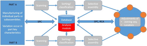
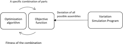
A new Digital Twin concept for the full production phase has been proposed by Söderberg et al. (2017). The procedure for this concept is shown in Figure 1.Based on that, the scanned data of individual parts A and B will be provided in the first step. Then, parts will be sorted and matched so that the variation of final assemblies becomes minimal. This technique is known as selective assembly. Afterward, the adjustment of locating schemes and welding sequences will be performed with the same goal in mind (Wärmefjord, Söderberg, and Lindkvist 2010). The concept of using selective assembly in Digital Twins and Cyber Factories are also suggested and discussed by Colledani et al. (2014) as a technique that improves the quality and cost of the production.

Figure 1. The proposed concept of Digital Twin for Geometry Assurance by Söderberg et al. (2017).

Although selective assembly technique is getting more attention in new production systems, application of this technique has been limited to small groups of assemblies and there is a gap in applying this technique to sheet metal assemblies. Section 1.1 provides a brief introduction to selective assembly and reviews the studies that has focused on this technique. Section 1.2, then, presents the existing gap and clarifies why this gap should be filled and how this study is going to fill it.

1.1. Selective assembly

Selective assembly is a means of obtaining higher quality product assemblies by using relatively low-quality components (Rezaei Aderiani, Wärmefjord, and Söderberg 2018). Therefore, quality improvement is the main advantage of implementing this technique. On the other hand, the drawback of using this technique is the added work for measuring the dimensions of all produced parts with high accuracy and sorting and matching parts before performing assembly. Nevertheless, these drawbacks can be compensated to a certain level by implementing the Digital Twin in the assembly line. Nowadays, it easier and cheaper to scan a sheet metal part compared to a decade ago. Moreover, automation is taking more place in production lines (Söderberg et al. 2017). The main assumption in a smart assembly line is that this trend will continue and in a near future, scanning all produced parts can be done even faster and cheaper than now (Söderberg et al. 2017). For instance, Bergström, Sjödahl, and Fergusson (2018) has developed an online shape inspection method that deviations of all produced parts from their nominal can be obtained just by taking some pictures from each part and analysing those pictures in a short time. Another assumption is that the assembly line will be robotised enough that the amount of time and workforce that will be added due to implementing selective assembly is reasonable. Considering these availabilities in near future, studying selective assembly technique for sheet metal makes a worthwhile contribution to the field.

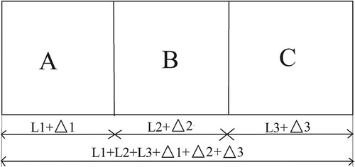
Figure 2 demonstrates an assembly of three components (in this paper, the word ‘components’ refers to the elements of an assembly and ‘parts’ refers to produced parts of that element for mass production). Suppose that the target of production is to produce 1000 of these assemblies and therefore, 1000 individual parts from each component are manufactured. After production, the longitudinal dimensions of the parts of component A, B and C will be measured. Hence, individual parts of each component will be divided into some groups (for instance six groups) based on their dimensions. Finally, the combination of groups that results in the minimal variation of the target dimensions in total assemblies can be obtained using different methods based on the circumstances of the problem. In other words, the optimal combination of $A_i$, $B_j$ and $C_k$ where $i,j,k\in \{1,2,3,\dots ,6\}$ should be found, so that variation of the longitudinal dimension among all assemblies is minimal. For instance, $\left(A_4{B}_1{C}_2\right)$, $\left(A_2{B}_5{C}_1\right)$, $\left(A_1{B}_2{C}_3\right)$, $\left(A_3{B}_4{C}_6\right)$, $\left(A_6{B}_6{C}_5\right)$ and $\left(A_5{B}_4{C}_4\right)$ can be an answer to this problem.

Figure 2. Sample of a linear assembly.

Dividing parts to groups and matching them was the primary method of applying selective assembly and has been used in bearing and engine production processes (Desmond and Setty 1961; Mansor 1961; Pugh 1992). In these types of assemblies, assembly tolerances are so tight that it becomes too expensive to obtain them by tightening part tolerances. However, since the groups selected to be assembled together may not contain the same number of parts, some parts in groups with a higher number of parts would be superfluous. These parts are known as surplus parts and this problem is called mismatching. Early studies in the area of selective assembly are mostly concerned with methods for making the groups so that mismatching becomes minimal (Fang and Zhang 1996, 1995; Chan and Linn 1998; Mease, Nair, and Sudjianto 2004).

Through the advent of evolutionary algorithms, including Genetic Algorithm (GA) and Simulated Annealing (SA), certain studies utilised these algorithms for selective assembly applications. Kannan, Jayabalan, and Jeevanantham (2003) utilised an integer coding GA to find the optimal combination of groups of parts aiming at minimising the variation in final assemblies. A chromosome is representative of a specific combination from all groups in this kind of coding. Then, each component has a substring in the chromosome and can embrace a sequence of integers. Each number is then allocated to a group number. This kind of coding is common in almost all studies that have used GA for selective assembly (Kannan, Asha, and Jayabalan 2005; Kumar and Kannan 2007; Asha, Kannan, and Jayabalan 2008; Kannan, Sivasubramanian, and Jayabalan 2009; Forslund et al. 2017; Rezaei Aderiani, Wärmefjord, and Söderberg 2018).

Most studies that deal with selective assembly by an evolutionary algorithm also present methodologies to solve the mismatching problem. Kannan, Asha, and Jayabalan (2005) presented a methodology to apply selective assembly in three stages to minimise the surplus parts. Rezaei Aderiani, Wärmefjord, and Söderberg (2018) developed a multistage approach to selective assembly that minimises the variation while the mismatching problem is solved and there are no surplus parts. Lanza, Haefner, and Kraemer (2015) investigated selective assembly by means of cyber-physical-based matching. Their study compares different strategies of selective assembly in term of total production costs in a cyber-physical factory. It shows that doing optimisation individually for all parts and not to divide them into different groups results in a lower cost of production.

1.2. Scope of paper

Implementing Digital Twins and cyber-physical factories are experiencing an upward trend in new production systems. These concepts can leverage selective assembly technique to minimise the production cost and improve the quality of the assembled product. The main type of assemblies in automotive industries are sheet metal assemblies which are assembled by spot welds. However, to the best of our knowledge, applying the concept of selective assembly in sheet metal assemblies has not been studied yet.

Studies of selective assembly have been limited to assemblies in which the target dimensions are just a function of some dimensions from mating parts. This paper refers to these types of assemblies as linear assemblies. The target dimensions in linear assemblies can be controlled by controlling dimensions of the mating parts by selecting them. In sheet metal assemblies, however, the final dimensions are not just function of dimensions of the mating parts. There is a large variety of other parameters including stiffness of sheets, welding properties and locating schemes of fixtures that affect the final geometry of the assembly. Hence, in a complex sheet metal assembly, the target dimensions cannot be defined as a function of sheets' dimensions. Consequently, the geometry cannot be controlled by some dimensions from mating parts, which is the base of common selective assembly techniques. Therefore, this question will raise that: is it possible to improve the final geometrical quality of sheet metal assemblies also by selecting the mating sheet metals instead of picking them randomly and assemble them? This is the primary question that this study tries to answer. In order to answer this question, a method for applying the selective assembly technique to sheet metal assemblies is required.

The differences between the essence of sheet metal assemblies and the linear assemblies necessitate some modifications on the existing methods of applying selective assembly technique. Therefore, another question that the paper answers is: What are those differences and the required modifications because of them? The answer of this question is covered in Sections 2 and 3.

The last question is then: If this technique can be applied to sheet metal assemblies, what would be the scale of the improvement and what are the effective parameters on the amount of improvement? The paper answers this question by applying the modified methodology in different batch sizes of three industrial cases. The results of this are presented in Section 4 and the effect of the batch size and future studies are discussed in Section 5.

2. Differences between linear and sheet metal assemblies and required modifications

A sheet metal assembly is usually made by putting two or more sheets of metal together that are joined by some spot welds, fasteners or seam welds. Spot weld joints are more common in automotive and aerospace industries and this paper deals with these types of joints.

Selective assembly of sheet metal shares the same concept as a conventional selective assembly. In both procedures, the parts that are going to be assembled together are selected instead of being randomly picked. However, the conventional selective assembly technique cannot be applied to the sheet metal assemblies as it is because of the differences that these types of assembly have with the linear assemblies. These differences and the required modifications that they imply are described here.

2.1. Lack of a single criterion for classifying parts into different groups

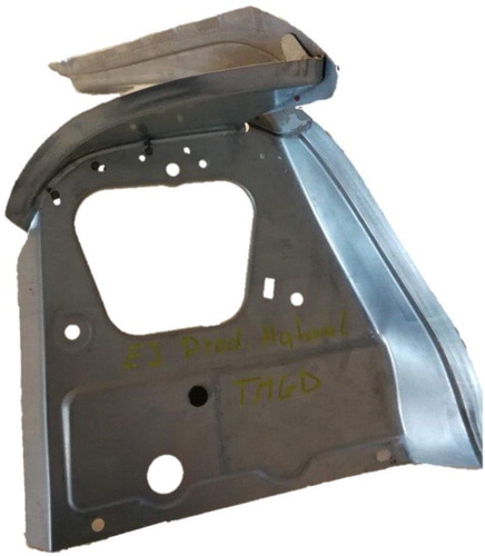
As it was mentioned in Section 1.1, in conventional selective assembly techniques, the parts are divided to some groups based on their measured dimension. However, it is not possible to apply this grouping to sheet metal parts. The geometrical outcome of a sheet metal assemblies is not only the function of some dimensions of their mating parts. As an example, an assembly from a car structure is shown in Figure 3.In this assembly, location of a point or variation of it cannot be attributed to dimensions of a specific point in the mating sheets. Each part is in contact with other parts in a contact area, and a couple of spot welds keep the parts together. Moreover, the locating scheme of fixtures, welding guns and other production parameters affect the geometry of the assembly. Therefore, there is not a single criterion to divide the parts based on that to different groups. As a result, the grouping procedure cannot be applied to these types of assemblies because there are not a single or a limited number of criteria on which to base the groups. For instance, suppose that the criteria for dividing sheets into groups is the deviation of a welding point of each individual part from its nominal position. Then, matching these groups to obtain less variation may not be possible because all parts in the same group would not have the same deviations in other areas of the part. Therefore, they would not have the same effect on the deviation of final assemblies. Consequently, the only alternative is to do the matching for each individual part instead of groups.

Figure 3. A sample sheet metal assembly.

2.2. Objective of selective assembly

In selective assembly for linear assemblies, the goal is to minimise the dimensional variation of all final assemblies. This is because variation is the only parameter in these kinds of assemblies that changes by changing the combination of the mating parts and the mean value of deviations is fixed. Consider a linear assembly that consists of two component x and y as an example. The dimension of the assembly that is going to be controlled by selective assembly is z which is summation or subtraction of x and y. This is shown in Equation (1(1) $z_i=x_i\pm y_i$(1) ) (Subtraction is applicable when the goal is to calculate the fit in a shaft and hole assembly). (1) $z_i=x_i\pm y_i$(1) Therefore, the mean value of z for all assemblies can be calculated from Equation (2(2) $Z=\frac{1}{N}\sum _{i=1}^N{z}_i$(2) ). (2) $Z=\frac{1}{N}\sum _{i=1}^N{z}_i$(2) By substituting Equation (1(1) $z_i=x_i\pm y_i$(1) ) into Equation (2(2) $Z=\frac{1}{N}\sum _{i=1}^N{z}_i$(2) ), the mean value can be determined based on the dimensions of the mating parts which is shown in Equation (3(3) $Z=\frac{1}{N}\sum _{i=1}^N(x_i\pm y_i)$(3) ). (3) $Z=\frac{1}{N}\sum _{i=1}^N(x_i\pm y_i)$(3) Based on Equation (3(3) $Z=\frac{1}{N}\sum _{i=1}^N(x_i\pm y_i)$(3) ), for linear assemblies the mean value of the assembly dimensions is not dependent on the combination of the mating parts. For example, if N is 2, Z would be the same for combination of $(x_1,y_1)(x_2,y_2)$ compared to combination of $(x_1,y_2)$ and $(x_2,y_1)$.

However, in sheet metal assemblies, the mean value of final assemblies' dimensions can vary when the combination of individual parts change. In other words, Equations (1(1) $z_i=x_i\pm y_i$(1) )–(3(3) $Z=\frac{1}{N}\sum _{i=1}^N(x_i\pm y_i)$(3) ) are not valid for sheet metal assemblies. For instance, if the assembly is a sheet metal assembly in the previous example, Z for combination of $(x_1,y_1)(x_2,y_2)$ may not be equal as Z for combination of $(x_1,y_2)$ and $(x_2,y_1)$. That is because in these types of assemblies there are more parameters rather than mating parts dimensions that affect the final dimensions and the relation of those factors with the final dimensions are not linear.

As a result, in selective assembly of sheet metals the mean value of deviation of a point or points can be considered as an objective of optimisation to be minimal in addition to the variation of these deviations. Hence, the problem changes from a single-objective optimisation to a multi-objective optimisation.

2.3. Relation between geometrical quality and mating parts

The other main difference is that the calculation of the final variation in sheet metal assemblies is not as easy as in linear assemblies. For the latter, the final dimensions can be calculated by some simple summations or subtractions of the dimension of these parts. Nevertheless, in order to predict the final deviations and variation of sheet metal assemblies, variation simulation analysis using Computer-Aided Tolerancing (CAT) tools is needed.

3. Method

Selective assembly is a combinatorial optimisation problem in which the objective is to minimise the final variation of manufactured assemblies.

As shown in Section 2.2, for sheet metal assemblies in addition to dimensional variation, the mean value of the deviation can be considered as the second objective to be minimal. To clarify the objectives, the definitions of geometrical variation and mean deviation in sheet metal assemblies are defined in Section 3.1. Thereafter, the formulation of the problem based on these objectives and the employed optimisation method to solve the problem are presented in Section 3.2. Afterward, two strategies of function evaluation are discussed in Section 3.3.

3.1. Objective function

The objective of optimisation in selective assembly of sheet metals is to minimise the geometrical variation and mean value of deviations. There are different ways of defining the variation for a parameter. One common definition in sheet metal assemblies in automotive industries is to measure the variation as six times the standard deviation. The definition of this parameter is shown in Equation (4(4) $6\sigma =6\sqrt{\frac{1}{N-1}\sum _{i=1}^N(d_i-\mu {)}^2}$(4) ). (4) $6\sigma =6\sqrt{\frac{1}{N-1}\sum _{i=1}^N(d_i-\mu {)}^2}$(4) where $\mu =\frac{1}{N}\sum _{i=1}^N{d}_i$ In this definition, N is the number of total assemblies, and $d_i$ is the magnitude of the deviation of a specific point from its nominal position after welding parts together and releasing the assembly from fixtures. To have a better view of the variation of the whole assembly, the continues surface of the sheets can be meshed to some elements. Then, the Root Mean Square (RMS) of variations and mean deviations in all elements can be considered as the objectives to be minimal. This is shown in Equations (5(5) $RM{S}_v=\sqrt{\frac{1}{n}\sum _{i=1}^n(6{\sigma }_i{)}^2}$(5) ) and (6(6) $RM{S}_m=\sqrt{\frac{1}{n}\sum _{i=1}^n({\mu }_i{)}^2}$(6) ). (5) $RM{S}_v=\sqrt{\frac{1}{n}\sum _{i=1}^n(6{\sigma }_i{)}^2}$(5) (6) $RM{S}_m=\sqrt{\frac{1}{n}\sum _{i=1}^n({\mu }_i{)}^2}$(6) where n is the number of elements in the assembly.

Deviation of a point in a sheet metal assembly can be predicted using variation simulation techniques or CAT (Wärmefjord et al. 2017). These techniques utilise Finite Element Method (FEM) to predict the deformation and spring back in the whole nodes of the model of the assembly. Moreover, implementing the Method of Influence Coefficient (MIC) reduces the calculation cost of the simulations (Liu and Hu 1997). This technique is also combined with contact modelling to improve accuracy (Wärmefjord et al. 2016). There are some commercial programs for this purpose such as RD&T (2018) and 3DCS (2018).

Deviation of all nodes, and therefore RMS of variation and the mean deviation for a specific number of assemblies, can be predicted by simulation using inspection data on the part level, joining process information, locating schemes and combination of parts as inputs.

This study utilises RD&T program as the variation simulation tool. This program does both rigid and non-rigid variation simulations; however, non-rigid simulation is utilised in this study. In non-rigid simulation, parts are allowed to deform when they are positioned. Hence, the stiffness of parts and clamping forces are considered in the simulation. Thus, the results are more reliable and accurate in non-rigid simulations (Wärmefjord et al. 2016).

Some assumptions are made in this tool for variation simulation including deformation is in the linear elastic range, fixtures and welding tools are rigid, the thermal deformations are negligible, materials are isotropic and stiffness matrix remains constant for deformed part shapes. The detailed procedure of the method of variation simulation that is utilised in RD&T is illustrated by Söderberg and Lindkvist (1999) and Lindkvist and Söderberg (2003).

3.2. Optimisation algorithm

Considering the objectives of optimisation as $RM{S}_m$ and $RM{S}_v$ from Equations (6(6) $RM{S}_m=\sqrt{\frac{1}{n}\sum _{i=1}^n({\mu }_i{)}^2}$(6) ) and (5(5) $RM{S}_v=\sqrt{\frac{1}{n}\sum _{i=1}^n(6{\sigma }_i{)}^2}$(5) ), the optimisation problem for selective assembly of sheet metals for two components can be formulated as Equation (7(7) $\begin{array}{rl}min& \left(\sqrt{\frac{1}{n}\sum _{k=1}^n{\left(\frac{1}{N}\sum _{i=1}^N\sum _{j=1}^N\left(d_{ijk}{x}_{ij}\right)\right)}^2},\sqrt{\frac{1}{n}\sum _{k=1}^n\left(\frac{36}{N-1}\sum _{i=1}^N\sum _{j=1}^N\left(x_{ij}{\left(d_{ijk}-\frac{1}{N}\sum _{i=1}^N\sum _{j=1}^N\left(d_{ijk}{x}_{ij}\right)\right)}^2\right)\right)}\right)\\ \mathrm{Subject}\mathrm{to}:& \sum _j^N{x}_{ij}=1;i=1,2,3\dots N\\ & \sum _i^N{x}_{ij}=1;j=1,2,3\dots N\\ & x_{ij}\in \{0,1\}\end{array}$(7) ). (7) $\begin{array}{rl}min& \left(\sqrt{\frac{1}{n}\sum _{k=1}^n{\left(\frac{1}{N}\sum _{i=1}^N\sum _{j=1}^N\left(d_{ijk}{x}_{ij}\right)\right)}^2},\sqrt{\frac{1}{n}\sum _{k=1}^n\left(\frac{36}{N-1}\sum _{i=1}^N\sum _{j=1}^N\left(x_{ij}{\left(d_{ijk}-\frac{1}{N}\sum _{i=1}^N\sum _{j=1}^N\left(d_{ijk}{x}_{ij}\right)\right)}^2\right)\right)}\right)\\ \mathrm{Subject}\mathrm{to}:& \sum _j^N{x}_{ij}=1;i=1,2,3\dots N\\ & \sum _i^N{x}_{ij}=1;j=1,2,3\dots N\\ & x_{ij}\in \{0,1\}\end{array}$(7) In this equation, $d_{ijk}$ is the deviation of the assembly in node k from its nominal, when part i from the first component and part j from the second component are mating parts of the assembly. Index n shows the number of all nodes and N represents the batch size (the number of parts). $x_{ij}$ is the optimisation variable and should be found by optimisation algorithm for all is and js. This variable represents the parts that are going to be assembled together from each component. For example, if $x_{54}$ is one, it means that part number 5 from the first component will be assembled to part number 4 from the second component. The constraints are applied to this variable so that it can only take zero or one and each row and each column can only have one one. These constraints make the optimisation combinatorial.

Selective assembly problem has been solved by a variety of optimisation algorithms. If the objective is to minimise the mean deviation, only in one point of the assembly, the problem will be a Linear Assignment Problem. In this situation, parts of one component can be considered as tasks and parts of the other component are the workers. The goal is to find the best match between tasks and workers so that the total cost is minimal and each worker takes only one task. The exact solution of this problem can be found using Hungarian or Auction Algorithm (Burkard, Dell'Amico, and Martello 2009). When the objective is to minimise the range of deviations of a point from its normal position, the problem will be a Bottleneck Assignment Problem (BAP) which can be solved in polynomial time using Threshold Algorithm (Burkard, Dell'Amico, and Martello 2009). However, considering $RM{S}_m$ and $RM{S}_v$ as objectives, selective assembly of sheet metals cannot be solved as an Assignment Problem. Because in this problem each node has a deviation that is different from other nodes and the goal is to minimise RMS of variation or mean deviation of all nodes.

Since the objective functions are non-linear and $x_{ij}$ is binary, selective assembly of sheet metals is a Mixed Integer Non-linear Programming (MINLP) problem. This optimisation problem can be solved using either metaheuristic optimisation algorithms or non-metaheuristic ones. Metaheuristic algorithms such as GA and SA are commonly used to solve this type of problems (Kannan, Asha, and Jayabalan 2005; Kumar, Kannan, and Jayabalan 2007; Asha, Kannan, and Jayabalan 2008; Rezaei Aderiani, Wärmefjord, and Söderberg 2018). Since the problem is multi-objective optimisation, Non-dominated Sorting Genetic Algorithm II (NSGA II) (Deb et al. 2002) can be utilised to find the optimal combination of parts.

An advantage of using non-metaheuristic methods is that exact solutions can be found while using metaheuristics there can not be a guarantee that the result is the global optimum. Moreover, metaheuristics suffer from the repeatability and reliability issues. On the other hand, a disadvantage of non-metaheuristics for solving combinatorial problems is that by increasing the size of the problem, the number of optimisation variables increases exponentially. Nevertheless, there is no such a problem when metaheuristics utilised to solve combinatorial problems (Blum and Roli 2003). Hence, if the size of the problem is too large to be solved by non-metaheuristics, the guarantee for finding the optimal solutions can be sacrificed for the sake of finding results that are good enough within a practical time (Blum and Roli 2003). For instance, for an assembly of 3 components with the batch size of 1000, the number of optimisation variables (size of $x_{ij}$) using non-metaheuristics will be one billion while this number is only 3000 using GA for combinatorial optimisations.

In this study, the sample cases are not too large to be solved using non-metaheuristics. In addition, the results are used to assess the effect of the batch size on the improvements. Therefore, this paper uses non-metaheuristics to solve the sample cases. There are some commercial solvers and toolboxes that can solve these types of problem. General Algebraic Modeling System (GAMS) program (Bussieck and Meeraus 2004) is utilised in this paper. This program encompasses some linear and non-linear solvers. To solve the optimisation problem in this paper DICOPT, CPLEX and CONOPT solvers are used in GAMS.

3.2.1. Multi-objective optimisation

This paper considers the optimisation problem as a multi-objective optimisation problem. The main reason is that depending on the quality requirements of the assembly and quality of produced parts, the quality engineers may give different priorities to $RM{S}_m$ and $RM{S}_v$. Therefore, having a Pareto-Front with different options to select among, gives more freedom to engineers to select based on the situation. However, if the priority of $RM{S}_m$ and $RM{S}_v$ over each other is known from the beginning, the problem can be converted to a single-objective optimisation, using a weighted sum of objectives as the objective function. A common combination of $RM{S}_m$ and $RM{S}_v$ that can also be used for single-objective optimisation is MSE and its definition is shown in Equation (8(8) $MSE=\frac{(RM{S}_m{)}^2+(RM{S}_v{)}^2}{6^2}$(8) ). (8) $MSE=\frac{(RM{S}_m{)}^2+(RM{S}_v{)}^2}{6^2}$(8) There are different methods of performing multi-objective optimizations with different advantages and disadvantages that are reviewed by Andersson (2000). This paper uses the ε-constraint method because of some advantages of it compared to other methods, especially in mixed integer problems that are discussed by Mavrotas (2009). In this method, the extremes of the Pareto-front can be obtained by solving a single-objective optimisation problem for each objective. Then, one objective will be considered to be minimal while the other objective is reformulated to a constraint as it is shown in Equation (9(9) $\begin{array}{rl}min& \left\{f_i\right\}\\ \mathrm{Subject}\mathrm{to}& f_j<{ϵ}_{j}i\ne j\end{array}$(9) ). Therefore, the other solutions in the Pareto-front can be obtained by changing ${ϵ}_j$ progressively. (9) $\begin{array}{rl}min& \left\{f_i\right\}\\ \mathrm{Subject}\mathrm{to}& f_j<{ϵ}_{j}i\ne j\end{array}$(9) The range of ${ϵ}_j$ is also defined according to the calculated extremes. In this paper, four solutions are calculated for each Pareto-front. The number of solutions can be different based on the user preference. Using this method, the extremes of $RM{S}_m$ and $RM{S}_v$ are calculated firstly, by solving one single-objective optimisation for each. Then, the range of $RM{S}_m$ is divided into three equal distances to have two $ϵs$. Afterward, two more single-objective optimisations are solved to minimise the $RM{S}_v$ while the constraint of $RM{S}_m<ϵ$ is added to the problem.

3.3. Strategies of function evaluation

The formulated optimisation problem of the selective assembly of sheet metals is presented in Equation (7(7) $\begin{array}{rl}min& \left(\sqrt{\frac{1}{n}\sum _{k=1}^n{\left(\frac{1}{N}\sum _{i=1}^N\sum _{j=1}^N\left(d_{ijk}{x}_{ij}\right)\right)}^2},\sqrt{\frac{1}{n}\sum _{k=1}^n\left(\frac{36}{N-1}\sum _{i=1}^N\sum _{j=1}^N\left(x_{ij}{\left(d_{ijk}-\frac{1}{N}\sum _{i=1}^N\sum _{j=1}^N\left(d_{ijk}{x}_{ij}\right)\right)}^2\right)\right)}\right)\\ \mathrm{Subject}\mathrm{to}:& \sum _j^N{x}_{ij}=1;i=1,2,3\dots N\\ & \sum _i^N{x}_{ij}=1;j=1,2,3\dots N\\ & x_{ij}\in \{0,1\}\end{array}$(7) ). In this equation, parameter $d_{ijk}$ is the deviation of nodes and will be calculated using the CAT program. No matter whether metaheuristic optimisation algorithms or non-metaheuristic are used to solve the problem, there are two strategies that can be followed to calculate the required $d_{ijk}s$ in each function evaluation.

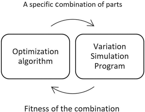
The first strategy is that the optimisation algorithm interacts with the simulation program. For each function evaluation, the optimisation algorithm calls the simulation program for calculating the required $d_{ijk}s$ and gets back the fitnesses of that combination of parts from the simulation program. The process of optimisation using this strategy is shown in Figure 4. Using this method, each function evaluation during the optimisation process requires one variation simulation.

Figure 4. Optimisation process using the first strategy.

The second strategy is to calculate the entire matrix of d firstly. Then, taking the required $d_{ijk}s$ for each function evaluation from that matrix. This procedure is shown in Figure 5.

Figure 5. Optimisation process using the second strategy.

Depending on the size d, one strategy can be selected for solving the problem. An advantage of using the first strategy is that it does not need to calculate the deviation of all nodes for every possible assembly. This is important when either the number of all possible assemblies or the number of nodes is too high so that it takes more time to calculate the deviation of all nodes for all possible assemblies compared to running a simulation for each function evaluation. On the other hand, the advantage of the second strategy is that it does not need to do simulation for each function evaluation. This leads to saving a considerable calculation time when calculating deviations of all possible assemblies in all nodes is plausible.

For instance, consider an assembly with two components and 10 parts for each component. The optimisation problem is to find the optimal combination of parts out of all possible combinations which are $10!$ combinations. The number of all possible assemblies in this example is ${10}^2=100$. Since the batch size (number of parts) is 10, $d_{ijk}$s of 10 assemblies will be called by the optimisation algorithm for each function evaluation. Therefore, if the number of function evaluations exceeds 10, using the first strategy of function evaluation leads to running more simulations than simulating all possible assemblies which are 100. Accordingly, in this case, the second strategy is superior compared to the first strategy. However, as an example of a large model, consider a model with 5 components and batch size of 1000. Then, the number of all possible assemblies is ${1000}^5$. Running this amount of simulations and then finding the optimal combination from those data is more time consuming than running 1000 simulation for each function evaluation since the number of function evaluations would be less than ${1000}^4$. Consequently, for this example, the first strategy is more reasonable. Since the presented sample cases in this paper are closer to the first example, the second strategy is implemented in this study.

4. Results

The method presented for selective assembly of sheet metals is applied to three different cases from the automotive industry and the results are evaluated. To implement the procedure using the second strategy of function evaluation, the matrix d is calculated for each problem using the RD&T program.

Different batch sizes of individual parts are considered for selective assembly to evaluate the effect of batch size on the improvement of each objective. These batch sizes for sample cases are considered to be 25, 50 and 100.

To be able to evaluate the amount of improvement in variation and mean deviation when selective assembly is applied, an average variation and mean deviation of a random assembly is needed. Hence, for each batch size, an average variation of 1000 random combinations of parts is calculated and considered. Replicating the calculation of average variation and mean deviation for 1000 random combinations shows that the difference between the calculated averages is less than 0.001. Therefore, 1000 random combination is enough for calculating the averages.

The first sample case is an assembly of three components from a car structure. This assembly is one of the most challenging assemblies in that car in terms of variation. The second sample case is an assembly of a door ring and door panel from a car and the third sample case is also an assembly of two sheet metal parts with spot welds.

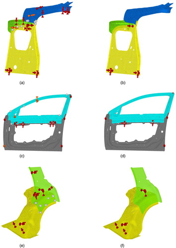
Each sheet metal part is modelled by shell elements. Contact elements between nodes in overlap areas are created to avoid penetration of parts. Figure 6 shows the models of these assemblies in RD&T. The white spheres in joint areas represent the spot welds between parts. The locating scheme of the assembly is applied to the models according to the locating scheme used in industry during assembly of these parts. The locators and support points that are applied to each part to position it before welding are shown in Figure 6(a,c,e) for sample cases 1, 2 and 3, respectively. After applying the welds, these locators are released and a new locating scheme is used to position the assembly during the inspection. In this locating scheme, the number of supports is reduced to a 3-2-1 locating scheme, which allows for spring-back. Figure 6(b,d,f) demonstrate the locating scheme of the assembly when the variation is measured for sample cases 1, 2 and 3, respectively. These locating schemes are based on the same locating scheme as in industry.

Figure 6. Models of sample cases in RD&T program. (a) Locating scheme of the first sample case before welding, (b) locating scheme of the first sample case for measurements, (c) locating scheme of the second sample case before welding, (d) locating scheme of the second sample case for measurements, (e) locating scheme of the third sample case before welding and (f) locating scheme of the third sample case for measurements.

The deformed individual parts of each component are imported into the simulation program in different batch sizes. Deformations of all deformed parts are in the range of the allowed tolerances. Having all deformed individual parts of components, deviation of nodes and the final variation can be calculated for different combinations of the parts using variation simulation. Then, the optimisation process is carried out and the combinations that result in minimal variations and mean deviations for all assemblies are obtained.

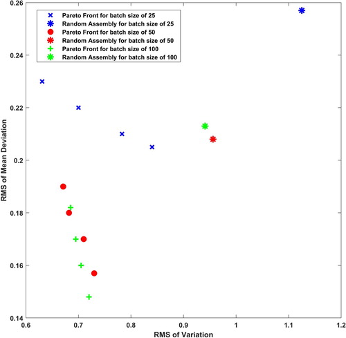
The Pareto-front and the average variations and mean deviations for different batch sizes sample case one are shown in Figure 7. The same results for sample case 2 and 3 are shown in Figures 8 and 9, respectively.

Figure 7. Pareto-Front and averages for different batch sizes of case 1.

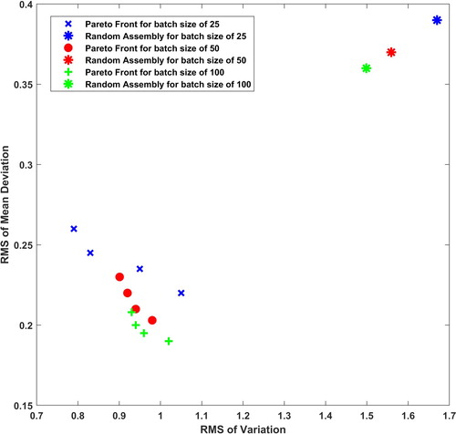
Figure 8. Pareto-Front and averages for different batch sizes of case 2.

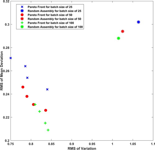
Figure 9. Pareto-Front and averages for different batch sizes of case 3.

The elapsed time for the entire procedure is divided into two parts. The first part is to calculate the matrix d using the simulation program. The second part is to solve the optimisation problem using GAMS. For all these cases, the elapsed time of the first part was less than 5 min using a PC with a Core i7 2.7 GHz CPU and 16 GB of RAM. The maximum elapsed time for the second part was 15 min using the same computation power to find one solution in the Pareto-front.

5. Discussion

The final variation of a sheet metal assembly is affected by a big variety of parameters that makes it complicated to sort and match parts based on them and apply selective assembly technique to their production. However, the results show that implementing the presented method is promising to reduce the variation and mean deviation of these assemblies.

Based on the results in Figures 7– 9, it seems like larger batch sizes have better Pareto-fronts. Nevertheless, each batch size has a different average of $RM{S}_v$ and $RM{S}_m$. Therefore, it is the percentage of improvement compared to average that should be evaluated to have a better judgment. Moreover, for the third sample case, the average and some solutions in the Pareto-front of the batch size 50 are better than for the batch size of 100. The reason for that is that the deformed parts considered for different batch sizes are different and there are no common deformed parts in different batches. Consequently, if some parts with larger deformation exist in a larger batch size that does not exist in smaller batch size, the smaller one can have a better average and Pareto-front.

5.1. Effect of batch size

To evaluate the effect of batch size, percentage of improvement of the variation and the mean deviation are presented in Figures 10 and 11, respectively. Each percentage in these charts is calculated by considering the difference between the minimal variation or deviation among all Pareto-Fronts and the average variation or the mean deviation.

Figure 10. Percentage of variation improvement compare to the average for different batch sizes of each case.

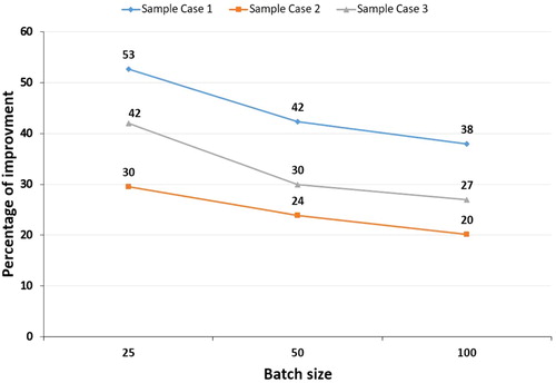
Figure 11. Percentage of mean value improvement compare to the average for different batch sizes of each case.

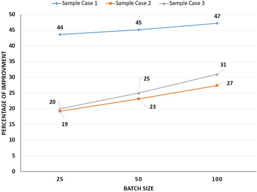
For all three sample cases, the percentage of improvement fell by increasing the batch size. It shows that the smaller the size of the batch, the higher the amount of improvement in average variation of that batch. On the other hand, Figure 11 shows that the percentage of improvement of the mean deviation improves for all cases by increasing the batch size.

These trends are due to the fact that the dimensional distributions are closer to the real-dimensional distribution for bigger batch sizes and smaller batch sizes represent a smaller area of the normal dimensional distributions. When the batch size is smaller, the variety of dimensions is less. This means that the final dimensions can be pushed to be in a smaller range. However, the mean value of that range is more deviated from the real mean value compare to the bigger batch sizes.

On the other hand, having additional parts imply a larger variety of deformed shapes. As a result, the range of dimensions that all assemblies can fit in them is confined by more parts. This is why the percentage of improvement of variation decreased for larger batch sizes. However, the mean values of bigger batch sizes can converge to values that are closer to the goal which results in higher improvements of the mean value for bigger batch sizes.

5.2. Future research

Selective assembly of sheet metals is a new area of research that needs to be improved upon in future research. Using a surrogate model in the second strategy of function evaluation for large models to reduce the time can be studied in future studies. Another area of future research is implementing deep learning algorithms in the process to see the results of applying the optimal combinations and modify the calculated combinations based on the production errors. The scope of this study is limited to the technical aspects of applying selective assembly to sheet metals. Therefore, further studies on logistic challenges would be extremely useful.

6. Conclusion

This paper presented selective assembly of sheet metals as a novel approach to selective assembly. The results show that geometrical variation and the mean deviation of sheet metal assemblies can be considerably improved by selecting the mating parts based on the scanned data of them. The differences between sheet metal assemblies and linear assemblies imply the following modifications on the existing approach of the selective assembly.

• The mean deviation of assemblies can be improved, in addition to variation of assemblies, by selective assembly in sheet metals. Therefore, the optimisation problem should change to multi-objective optimisation problem.

• Because of the complexity of sheet metal assemblies compare to linear assemblies, it is not practical to divide parts into groups and the matching should be done for individual parts.

• Variation simulation tools should be utilised to calculate the objectives of the optimisation process.

The amount of improvement and effect of batch size on that are also investigated. Based on the results, the amount of improvement is subjective and depends on the case. However, the applied cases show that the improvement in variation and the mean deviation can be up to 53 %. It can be concluded that increasing the batch size results in a higher percentage of improvement in the mean deviation and lower percentage of improvement in variation.

Disclosure statement

No potential conflict of interest was reported by the authors.

ORCID

Abolfazl Rezaei Aderiani  http://orcid.org/0000-0002-2720-9838

Kristina Wärmefjord  http://orcid.org/0000-0003-1556-3319

Rikard Söderberg  http://orcid.org/0000-0002-9138-4075

Lars Lindkvist  http://orcid.org/0000-0002-6575-5098

Additional information

Funding

This work was carried out in collaboration within Wingquist Laboratory and the Area of Advance Production at Chalmers within the project Smart Assembly 4.0, financed by the Swedish Foundation for Strategic Research (Stiftelsen för Strategisk Forskning). Their support is gratefully acknowledged.

References

- Andersson, Johan. 2000. “A Survey of Multiobjective Optimization in Engineering Design Johan.”
- Asha, A., S. M. Kannan, and V. Jayabalan. 2008. “Optimization of Clearance Variation in Selective Assembly for Components with Multiple Characteristics.” International Journal of Advanced Manufacturing Technology 38: 1026–1044. doi: 10.1007/s00170-007-1136-3
- Bergström, Per, Mikael Sjödahl, and Michael Fergusson. 2018. “Virtual Projective Shape Matching in Targetless CAD-based Close-range Photogrammetry for Efficient Estimation of Specific Deviations.” Optical Engineering 57 (5): 053110. https://doi.org/10.1117/1.OE.57.5.053110.
- Blum, Christian, and Andrea Roli. 2003. “Metaheuristics in Combinatorial Optimization: Overview and Conceptual Comparison.” ACM Computing Surveys 35 (3): 268–308. http://doi.acm.org/10.1145/937503.937505.
- Burkard, Rainer, Mauro Dell'Amico, and Silvano Martello. 2009. Assignment Problems. Philadelphia, PA: Society for Industrial and Applied Mathematics.
- Bussieck, Michael R., and Alexander Meeraus. 2004. “General Algebraic Modeling System (GAMS).” In Modeling Languages in Mathematical Optimization, edited by J. Kallrath, Vol. 88 of Applied Optimization, 137–157. Springer, Boston, MA. https://doi.org/10.1007/978-1-4613-0215-5_8.
- Chan, Ka Ching, and Richard J. Linn. 1998. “A Grouping Method for Selective Assembly of Parts of Dissimilar Distributions.” Quality Engineering 11 (2): 221–234. doi: 10.1080/08982119808919233
- Colledani, Marcello, Tullio Tolio, Anath Fischer, Benoit Iung, Gisela Lanza, Robert Schmitt, and József Váncza. 2014. “Design and Management of Manufacturing Systems for Production Quality.” CIRP Annals – Manufacturing Technology 63 (2): 773–796. doi: 10.1016/j.cirp.2014.05.002
- 3DCS. 2018. “DCS web page.” http://www.3dcs.com.
- Deb, K., A. Pratap, S. Agarwal, and T. Meyarivan. 2002. “A Fast and Elitist Multiobjective Genetic Algorithm: NSGA-II.” IEEE Transactions on Evolutionary Computation 6 (2): 182–197. doi: 10.1109/4235.996017
- Desmond, D. J., and C. A. Setty. 1961. “Simplification of Selective Assembly.” International Journal of Production Research 1 (3): 3–18. doi: 10.1080/00207546108943085
- Fang, X. D., and Y. Zhang. 1995. “A New Algorithm for Minimising the Surplus Parts in Selective Assembly.” Computers and Industrial Engineering 28 (2): 341–350. doi: 10.1016/0360-8352(94)00183-N
- Fang, X. D., and Y. Zhang. 1996. “Assuring the Matchable Degree in Selective Assembly Via a Predictive Model Based on Set Theory and Probability Method.” Journal of Manufacturing Science Engineering118: 252–258. doi: 10.1115/1.2831018
- Forslund, A., S. Lorin, L. Lindkvist, K. Wärmefjord, and R. Söderberg. 2017. “Minimizing Weld Variation Effects using Permutation Genetic Algorithms and Virtual Locator Trimming.” ASME International Mechanical Engineering Congress and Exposition, Proceedings (IMECE) 2.
- Glaessgen, Edward, and David Stargel. 2012. “The Digital Twin Paradigm for Future NASA and US Air Force Vehicles.” 53rd Structural Dynamics and Materials ConferenceBR 20th AIAA/ASME/AHS Adaptive Structures Conference 14th AIAA, Honolulu, Hawaii.
- Kannan, Soma M., A. Asha, and V. Jayabalan. 2005. “A New Method in Selective Assembly to Minimize Clearance Variation for a Radial Assembly Using Genetic Algorithm.” Quality Engineering 17 (4): 595–607. doi: 10.1080/08982110500225398
- Kannan, S. M., V. Jayabalan, and K. Jeevanantham. 2003. “Genetic Algorithm for Minimizing Assembly Variation in Selective Assembly.” International Journal of Production Research 41 (14): 3301–3313. doi: 10.1080/0020754031000109143
- Kannan, S. M., R. Sivasubramanian, and V. Jayabalan. 2009. “A New Method in Selective Assembly for Components with Skewed Distributions.” International Journal of Productivity and Quality Management 4 (5/6): 569. doi: 10.1504/IJPQM.2009.025186
- Kumar, M. Siva, and S. M. Kannan. 2007. “Optimum Manufacturing Tolerance to Selective Assembly Technique for Different Assembly Specifications by Using Genetic Algorithm.” International Journal of Advanced Manufacturing Technology 32 (5–6): 591–598. doi: 10.1007/s00170-005-0337-x
- Kumar, M. Siva, S. M. Kannan, and V. Jayabalan. 2007. “A New Algorithm for Minimizing Surplus Parts in Selective Assembly by Using Genetic Algorithm.” International Journal of Production Research 45 (20): 4793–4822. doi: 10.1080/00207540600810085
- Lanza, Gisela, Benjamin Haefner, and Alexandra Kraemer. 2015. “Optimization of Selective Assembly and Adaptive Manufacturing by Means of Cyber-physical System Based Matching.” CIRP Annals – Manufacturing Technology 64 (1): 399–402. doi: 10.1016/j.cirp.2015.04.123
- Lindkvist, Lars, and Rikard Söderberg. 2003. “Computer-aided Tolerance Chain and Stability Analysis.” Journal of Engineering Design 14 (1): 17–39. doi:10.1080/0954482031000078117.
- Liu, S. C., and S. J. Hu. 1997. “Variation Simulation for Deformable Sheet Metal Assemblies Using Finite Element Methods.” Journal of Manufacturing Science and Engineering, Transactions of the ASME 119 (3): 368–374. doi: 10.1115/1.2831115
- Mansor, E. M. 1961. “Selective Assembly-its Analysis and Applications.” International Journal of Production Research 1 (1): 13–24. doi: 10.1080/00207546108943070
- Mavrotas, George. 2009. “Effective Implementation of the E-constraint Method in Multi-Objective Mathematical Programming Problems.” Applied Mathematics and Computation 213 (2): 455–465. http://www.sciencedirect.com/science/article/pii/S0096300309002574. doi: 10.1016/j.amc.2009.03.037
- Mease, David, Vijayan N. Nair, and Agus Sudjianto. 2004. “Selective Assembly in Manufacturing: Statistical Issues and Optimal Binning Strategies.” Technometrics 46 (2): 165–175. doi: 10.1198/004017004000000185
- Pugh, G. Allen. 1992. “Selective Assembly with Components of Dissimilar Variance.” Computer and Industrial Engineering 23 (1–4): 487–491. doi: 10.1016/0360-8352(92)90167-I
- RD&T. 2018. “RD&T Technology.” http://rdnt.se/.
- Rezaei Aderiani, Abolfazl, Kristina Wärmefjord, and Rikard Söderberg. 2018. “A Multistage Approach to the Selective Assembly of Components Without Dimensional Distribution Assumptions.” Journal of Manufacturing Science and Engineering 140 (7): 071015. doi:10.1115/1.4039767.
- Söderberg, Rikard, and Lars Lindkvist. 1999. “Computer Aided Assembly Robustness Evaluation.” Journal of Engineering Design 10 (2): 165–181. doi:10.1080/095448299261371.
- Söderberg, Rikard, Kristina Wärmefjord, Johan S. Carlson, and Lars Lindkvist. 2017. “Toward a Digital Twin for Real-time Geometry Assurance in Individualized Production.” CIRP Annals – Manufacturing Technology 66 (1): 137–140. doi: 10.1016/j.cirp.2017.04.038
- Tuegel, Eric J., Anthony R. Ingraffea, Thomas G. Eason, and S. Michael Spottswood. 2011. “Reengineering Aircraft Structural Life Prediction using a Digital Twin.” International Journal of Aerospace Engineering 2011 (1), Article ID 154798, 14 pages. https://doi.org/10.1155/2011/154798.
- Wärmefjord, Kristina, Rikard Söderberg, Björn Lindau, Lars Lindkvist, and Samuel Lorin. 2016. “Joining in Nonrigid Variation Simulation.” In Computer-aided Technologies – Applications in Engineering and Medicine, edited by R. Udroiu, IntechOpen, Rijeka. https://doi.org/10.5772/65851.
- Wärmefjord, Kristina, Rikard Söderberg, and Lars Lindkvist. 2010. “Strategies for Optimization of Spot Welding Sequence With Respect to Geometrical Variation in Sheet Metal Assemblies.” Volume 3: Design and Manufacturing, Parts A and B (November 2015): 569–577. Vancouver, British Columbia, Canada. doi:10.1115/IMECE2010-38471.
- Wärmefjord, Kristina, Rikard Söderberg, Lars Lindkvist, Björn Lindau, and Johan S. Carlson. 2017. “Inspection Data to Support a Digital Twin for Geometry Assurance.” Volume 2: Advanced Manufacturing V002T02A101, Tampa, Florida, USA. doi:10.1115/IMECE2017-70398.