Sustainable operations of industrial symbiosis: an enterprise input-output model integrated by agent-based simulation

Abstract

Industrial symbiosis (IS) is a key for implementing circular economy. Through IS, wastes produced by one company are used as inputs by other companies. The operations of IS suffers from uncertainty barriers since wastes are not produced upon demand but emerge as secondary outputs. Such an uncertainty, triggered by waste supply-demand quantity mismatch, influences IS business dynamics. Accordingly, companies have difficulty to foresee potential costs and benefits of implementing IS. The paper adopts an enterprise input-output model providing a cost–benefit analysis of IS integrated to an agent-based model to simulate how companies share the total economic benefits stemming from IS. The proposed model allows to explore the space of cooperation, defined as the operationally favourable conditions to operate IS in an economically win-win manner. This approach, as a decision-support tool, allows the user to understand whether the IS relationship is created and how should the cost-sharing policy be. The proposed model is applied to a numerical example. Findings show that cost-sharing strategies are dramatically affected by waste supply-demand mismatch and by the relationship between saved and additional costs to run IS. Apart from methodological and theoretical contributions, the paper proposes managerial and practical implications for business strategy development in IS.

Keywords:

• Industrial symbiosis
• enterprise input-output
• sustainable operations
• agent-based simulation
• circular economy

1. Introduction

Environmental sustainability has become the reference issue of any development programme since the attention towards the continuous deterioration of the environment and the unsustainable pattern of consumption and production have been increasing (Mathiyazhagan, Govindan, and Noorul Haq 2014; European Commission 2015). Improving efficiency and sustainability of production processes enables the shift towards sustainable production and consumption (e.g. Kumar, Teichman, and Timpernagel 2012; Govindan, Jha, and Garg 2016). In fact, there is the need to give further impetus to efficient and eco-innovative production processes, to reduce dependency on raw materials, and to encourage optimal resource use and recycling within the context of circular economy (e.g. European Commission 2015; Murray, Skene, and Haynes 2017; Govindan and Hasanagic 2018; Sarkis and Zhu 2018).

The industrial symbiosis (IS) is considered as a key practice for the transition towards the circular economy (e.g. Abreu and Ceglia 2018; Saavedra et al. 2018). An IS relationship between two companies occurs when a waste produced by the former is used to replace a traditional production input by the latter (Chertow 2000; Lombardi and Laybourn 2012). This allows companies to reduce the amounts of both wastes discharged in landfills and virgin inputs used in production processes, leading to direct environmental benefits for the overall society (e.g. Jacobsen 2006; Mattila, Pakarinen, and Sokka 2010). In turn, these benefits trigger indirect and induced benefits such as reductions in greenhouse gas (GHG) emissions and energy consumption (e.g. Martin, Svensson, and Eklund 2015; Kim et al. 2018). However, the literature widely acknowledges that companies are pushed to explore IS opportunities by the potential economic benefit from IS, which stem from the avoided waste discharge and primary input purchase costs, net of the additional cooperation costs of operating the IS relationship (e.g. waste transportation and treatment costs) (e.g. Esty and Porter 1998; Lyons 2007; Yuan and Shi 2009; Xiong et al. 2017).

An IS-based business takes place in three phases: identification of the IS opportunity and potential business partners, assessment of the potential economic benefits, and implementation of the business. Several tools aimed at facilitating IS identification have been developed (e.g. Cutaia et al. 2014; Low et al. 2018; Maqbool, Mendez Alva, and Van Eetvelde 2018; van Capelleveen, Amrit, and Yazan 2018). However, scant attention has been devoted at developing tools that support companies in assessing and implementing a potential IS-based business from operational and managerial perspectives. This paper particularly addresses this gap.

Concerning the implementation phase, for each company a minimum economic benefit motivating it towards the IS practice exists, which mainly depends on the desired return on investment (e.g. Mirata 2004). Hence, an IS relationship between two companies can be successfully established only if both companies achieve an economic benefit sufficient to motivate them towards the cooperation (the so-called win-win condition). In this regard, the literature provided some contributions on how to align the incentives for the symbiotic cooperation by making an IS relationship convenient enough for both of the involved companies – see, for instance, the models to fairly share the additional costs of IS (Yazdanpanah and Yazan 2017) and to design the contractual clauses related to the waste exchange (Albino, Fraccascia, and Giannoccaro 2016). However, the above-mentioned contributions have been proven to be effective only in case of quantity match between supply and demand of wastes. Expectedly, a perfect quantity match between waste supply and demand hardly occurs, since wastes are not produced upon demand but emerge as secondary outputs of the main production activities (Yazan, Romano, and Albino 2016). This situation might lead to operational uncertainties to run the IS over time and can exacerbate the incentive misalignment between the involved companies (e.g. Chopra and Khanna 2014; Fraccascia, Giannoccaro, and Albino 2017b). In fact, if the demand (supply) for waste is higher than the produced (required) amount, the waste user (producer) might gain a scant economic benefit, which may not be enough to be motivated towards the cooperation¹ (Albino, Fraccascia, and Giannoccaro 2016). Hence, companies need practical tools providing support on how to deal with such a quantity mismatch.

To the best of our knowledge, this is the first paper to this aim. This paper first develops a cost–benefit analysis model that assesses the potential economic benefits from an IS relationship under specific quantity mismatch scenarios. The model is based on the Enterprise Input-Output (EIO) approach (e.g. Lin and Polenske 1998; Grubbstrom and Tang 2000). Then, this cost–benefit model is integrated to an agent-based model (e.g. Axelrod 1997; Bonabeau 2002) that simulates how the involved companies negotiate the contractual clauses for sharing the additional costs to operate IS. The proposed model explores the space of cooperation, which represents the operationally favourable conditions to launch and operate an IS-based business in an economically win-win manner. This approach allows companies to understand in which quantity mismatch scenarios an IS relationship might be created and – in case the relationship is created – how should the cost-sharing policy be.

A numerical example concerning the use of marble waste in concrete production (e.g. Hebhoub et al. 2011) is used to show how the model works via computational experiments (e.g. Ghodsypour and O’Brien 1998; Hill 1999; Sabri and Beamon 2000; Ghodsypour and O’Brien 2001; Chan 2003). Several quantity (mis-)match scenarios are analyzed. By simulating each scenario for 10,000 times, the following are computed: (1) the probability that the IS relationship is created; and (2) the percentage of additional costs paid by each company. In the model, input purchase cost, waste discharge cost, and additional costs for operating IS are considered as the main factors influencing the space of cooperation. The impact of these factors on the space of cooperation is investigated via sensitivity analysis.

The paper is structured as follows: Section 2 provides a theoretical background on the two methodologies, i.e. EIO modelling and Agent-Based Modelling. The EIO model and the Agent-Based model for IS are described in Section 3. Section 4 presents the numerical example together with the results of the computational experiments. Findings are discussed in Section 5 and conclusions are drawn in Section 6.

2. Methodological background

This section provides a theoretical background on the two methodologies used in this paper: the Enterprise Input-Output (EIO) approach (Section 2.1) and the Agent-Based modelling (ABM) (Section 2.2).

2.1. Enterprise input-output models

Enterprise Input-Output (EIO) models are a specific set of Input-Output models, helpful to complement the managerial and financial accounting systems used by firms (Grubbstrom and Tang 2000). EIO models are useful as a planning and accounting tool to map the physical (material, energy, water) and monetary flows among production processes at different levels: (1) inside one company; (2) among different companies involved in a supply chain; (3) among different companies that belong to different supply chains. In particular, EIO models are useful to analyze and manage internal and external logistics flows, as well as to support coordination policies among different production processes and companies. Furthermore, EIO models are suitable for assessing direct and indirect environmental impacts of production processes and supply chains, since the EIO approach accounts for production inputs as well as wastes and by-products of production processes. The literature provides several applications of the EIO approach in the industrial context. First, Lin and Polenske (1998) propose a specific EIO model to map the material, energy, and waste flows of a steel plant. Subsequently, several models analyzing materials and energy flows in global and local supply chains and industrial districts have been proposed (e.g. Albino, Dietzenbacher, and Kühtz 2003; Kuhtz et al. 2010; Liang, Jia, and Zhang 2011; Tan et al. 2016; Yazan, Mandras, and Garau 2017).

EIO models are valuable tools for analyzing physical and monetary flows in IS. In fact, they have several advantages compared to other methodologies used in the IS context (e.g. material flow analysis): (1) instead of just highlighting waste flows among processes and companies, they are able to model drivers of waste production and demand; (2) they are able to model waste flows as directly dependent on demand and production of wastes; (3) they can simultaneously analyze physical and monetary flows among companies; and (4) they can model monetary flows taking into account the contractual clauses negotiated between companies. For these reasons, EIO models have been recently adopted in the IS context for several aims. Fraccascia, Albino, and Garavelli (2017) discuss the extent to which companies can enhance the technical efficiency of their production processes by adopting the IS practice. Yazan, Romano, and Albino (2016) investigate the factors influencing the match between demand and supply of wastes in IS relationships. Albino, Fraccascia, and Giannoccaro (2016) model the physical and monetary flows created among firms within an IS network while Benjamin, Tan, and Razon (2015) and Tan et al. (2016) study how these flows can be vulnerable to perturbations over time. Yazan (2016) investigates joint production chains (JPC) constructed via IS and computes the holistic supply chain impacts (in terms of material and energy savings) within the JPCs triggered by the IS practice. Zhang, Du, and Wang (2018) propose an EIO model to compute the reductions in carbon footprint thanks to the IS practice. Fraccascia, Giannoccaro, and Albino (2017a) compute monetary flows between firms and governments thanks to environmental policy actions aimed at supporting the implementation of IS practices. However, to the best of our knowledge, no EIO models providing cost–benefit analysis in IS relationships have been developed in the literature. This paper carries out a cost–benefit analysis based on the EIO model.

2.2. Agent-based modelling

Agent-based modelling (ABM) is one of the most suited techniques to study complex systems composed of different entities interacting among each other. Each entity is modelled as an agent, which is provided with a given set of goals to accomplish through the interaction with the other agents and the environment, driven by a given set of rules of social engagement (Weiss 1999; Bonabeau 2002; Holland 2002). The main goal of the agent-based simulation is to enrich our understanding of some fundamental processes and to build new theories, concepts, and knowledge about these processes (Epstein and Axtell 1996; Axelrod 1997; Carley and Gasser 1999). Compared to traditional simulations techniques, the outcomes of agent-based simulation arise from the spontaneous interaction among agents without being externally imposed on the system (Goldstein 1999). This characteristic makes the ABM approach particularly suited to study cooperation dynamics among firms within supply chains and industrial districts (e.g. Giannoccaro 2015; Yu, Wong, and Li 2017; Giannoccaro, Nair, and Choi 2018). Based on the above, such an approach is considered appropriate to analyze the dynamics of symbiotic cooperation (Batten 2009; Romero and Ruiz 2014). In fact, agent-based models were recently adopted to explore the creation process of self-organized IS networks, and in particular the role played on this process by benefit-sharing contracts (Albino, Fraccascia, and Giannoccaro 2016), regulations (Fraccascia, Giannoccaro, and Albino 2017a), online information-sharing platforms (Fraccascia and Yazan 2018), and social and behavioural factors (Bichraoui, Guillaume, and Halog 2013; Ghali, Frayret, and Ahabchane 2017; Zheng and Jia 2017). Furthermore, other studies focus on the evolution process of IS networks over time (Cao, Feng, and Wan 2009; Ashton, Chopra, and Kashyap 2017). Different than the above-mentioned models, the agent-based model proposed in this paper uses the outcome of the EIO-based cost–benefit analysis to simulate the negotiation for cost-sharing between companies involved in an IS relationship.

3. Methods

This section is divided into two subsections. First, the Enterprise Input-Output (EIO) model for cost–benefit analysis of IS relationships is presented in Section 3.1. Then, the agent-based model used for simulation is presented in Section 3.2.

3.1. The enterprise input-output model for cost–benefit analysis

In order to build our analytical model, let us consider two production processes owned by two independent companies, α and β. For the sake of simplicity, let us assume that each process produces one main output, α generates one waste, and β requires one primary input. The amount of waste produced by α (i.e. $w^{\alpha }$) and the amount of primary input required by β (i.e. $r^{\beta }$) depend on the amount of main outputs produced by these firms (triggered by the market demand) as well as on the production technology. Accordingly: (1) $w^{\alpha }=W^{\alpha }{x}^{\alpha }$(1) (2) $r^{\beta }=R^{\beta }{x}^{\beta }$(2) where $x_{}^{\alpha }$ and $x_{}^{\beta }$ denote the amount of main outputs produced by α and β, respectively, and $W^{\alpha }$ and $R^{\beta }$ are technical coefficients representative for production technologies. In particular, $W^{\alpha }$ denotes the waste production rate of α, i.e. how many units of waste are generated by α per unit of main output. Similarly, $R^{\beta }$ denotes the input consumption rate of β, i.e. how many units of primary input are required by β per unit of main output. The lower the values of $W^{\alpha }$ and $R^{\beta }$, the more the adopted production processes are technically efficient and environmentally friendly, ceteris paribus (Fraccascia, Albino, and Garavelli 2017). Values of $x_{}^{\alpha }$, $x_{}^{\beta }$, $W^{\alpha }$, and $R^{\beta }$ can change over time. In particular, changes on $x_{}^{\alpha }$ and $x_{}^{\beta }$ can be triggered by the market demand for main products of α and β, respectively, while changes on $W^{\alpha }$ and $R^{\beta }$ are possible as a result of technological innovation (e.g. Sonis and Hewings 2007; Yazan, Romano, and Albino 2016). In this regard, if α upgrades its production process so that its waste production rate is decreased, the value of $W^{\alpha }$ is reduced. Similarly, if β upgrades its production process so that its input consumption rate is decreased, the value of $R^{\beta }$ is reduced. According to Equations 1 and 2, these changes can be responsible for fluctuations in the amount of produced wastes and required inputs.

From the symbiotic perspective, let us assume that the waste produced by α can be used by β to replace its primary input. Furthermore, for the sake of simplicity, let us assume that one unit of waste is able to replace one unit of primary input. Two different scenarios, A and B, can be considered.

In scenario A, the firms do not cooperate, i.e. no industrial symbiosis (IS) relationship occurs. In this case, α discharges $w^{\alpha }$ units of waste in the landfill l and β purchases $r^{\beta }$ units of primary input from conventional supplier s. Discharge costs paid by α (i.e. $C_{w^{\alpha }}^A$) are computed as follows: (3) $C_{w^{\alpha }}^A=(C_{w^{\alpha }}^l+C_{w^{\alpha }}^{\alpha l})\cdot w^{\alpha }$(3) where $C_{w^{\alpha }}^l$ denotes the discharge cost per unit of $w^{\alpha }$ and $C_{w^{\alpha }}^{\alpha l}$ denotes the cost to transport one unit of $w^{\alpha }$ from α to the landfill. These costs may depend on several factors, e.g. the market prices for discharge, the distance between the company and the landfill, the market prices of transportation service, regulations over the waste discharge (e.g. Costa and Ferrão 2010; Tao et al. 2019). Primary input purchase costs paid by β, i.e. $C_{r^{\beta }}^A$, are computed as follows: (4) $C_{r^{\beta }}^A=(C_{r^{\beta }}^s+C_{r^{\beta }}^{s\beta })\cdot r^{\beta }$(4) where $C_{r^{\beta }}^s$ denotes the cost of purchasing one unit of $r^{\beta }$ from the conventional supplier s and $C_{r^{\beta }}^{s\beta }$ denotes the cost of transporting one unit of $r^{\beta }$ from s to β. These costs may be influenced by, e.g. the market prices of the primary resource, the transportation distance between the company and the supplier, the market prices of the transportation service. Thus, the total cost of scenario A, i.e. C^A, is: (5) $C^A=C_{w^{\alpha }}^A+C_{r^{\beta }}^A$(5) Scenario B is characterised by the symbiotic cooperation among firms, i.e. the waste generated by α is used to replace the primary input required by β. In this case, waste discharge costs and input purchase costs are reduced. However, these economic benefits are eroded by the additional costs required to manage the IS relationship, in particular waste transportation and treatment costs, i.e. the costs to make the waste available to be used as input. According to the different quantity of $w^{\alpha }$ produced and $r^{\beta }$ required, three situations may occur, i.e.: (1) $w^{\alpha }<r^{\beta }$, (2), $w^{\alpha }>r^{\beta }$, and (3) $w^{\alpha }=r^{\beta }$. They are analyzed as follows.

If $w^{\alpha }<r^{\beta }$, the overall amount of waste is used to replace the primary input. Hence, α does not discharge any unit of waste whilst β still purchases $r^{\beta }-w^{\alpha }$ units of primary input from the conventional supplier. The additional costs arising from the IS relationship (i.e. $C_{w^{\alpha }{r}^{\beta }}^B$) and the costs to purchase the remaining amount of primary input (i.e. $C_{r^{\beta }}^B$) are respectively computed as follows: (6) $C_{w^{\alpha }{r}^{\beta }}^B=C_{w^{\alpha }{r}^{\beta }}^{\alpha \beta }\cdot w^{\alpha }$(6) (7) $C_{r^{\beta }}^B=(C_{r^{\beta }}^s+C_{r^{\beta }}^{s\beta })(r^{\beta }-w^{\alpha })$(7) where $C_{w^{\alpha }{r}^{\beta }}^{\alpha \beta }$ denotes the total additional cost required to exchange one unit of $w^{\alpha }$ between α and β. This cost may be influenced by the distance between companies, the type of exchanged waste, and the market price for transportation service (e.g. Domenech et al. 2019).

If $w^{\alpha }>r^{\beta }$, the overall amount of input is replaced by waste. Hence, β does not purchase any unit of primary input from the conventional supplier whilst α still discharges $w^{\alpha }-r^{\beta }$ units of waste in the landfill. The additional costs arising from the IS relationship and the costs to discharge the remaining amount of waste (i.e. $C_{w^{\alpha }}^B$) are computed as follows: (8) $C_{w^{\alpha }{r}^{\beta }}^B=C_{w^{\alpha }{r}^{\beta }}^{\alpha \beta }\cdot r^{\beta }$(8) (9) $C_{w^{\alpha }}^B=(C_{w^{\alpha }}^l+C_{w^{\alpha }}^{\alpha l})(w^{\alpha }-r^{\beta })$(9) Finally, if $w^{\alpha }=r^{\beta }$, there is a perfect match between the amount of produced waste and the amount of required input. Hence, α does not discharge any unit of waste and β does not purchase any unit of input from the conventional supplier. Only $C_{w^{\alpha }{r}^{\beta }}^B$occurs.

The total cost associated with scenario B is computed as follows: (10) $C^B=\left\{\begin{array}{ccc}{C}_{w^{\alpha }{r}^{\beta }}^B+C_{r^{\beta }}^B& \text{if}& w^{\alpha }<r^{\beta }\\ C_{w^{\alpha }{r}^{\beta }}^B+C_{w^{\alpha }}^B& \text{if}& w^{\alpha }>r^{\beta }\\ C_{w^{\alpha }{r}^{\beta }}^B& \text{if}& w^{\alpha }=r^{\beta }\end{array}\right.$(10) The overall economic benefit of the cooperation is computed as the cost reduction thanks to the IS, i.e. as ${\mathrm{\Delta }}_{AB}=C^A-C^B$. In particular: (11) ${\mathrm{\Delta }}_{AB}=\left\{\begin{array}{ccc}\left[\left(C_{w^{\alpha }}^l+C_{w^{\alpha }}^{\alpha l}\right)+\left(C_{r^{\beta }}^s+C_{r^{\beta }}^{s\beta }\right)-C_{w^{\alpha }{r}^{\beta }}^{\alpha \beta }\right]\cdot w^{\alpha }& \text{if}& w^{\alpha }\le r^{\beta }\\ \left[\left(C_{w^{\alpha }}^l+C_{w^{\alpha }}^{\alpha l}\right)+\left(C_{r^{\beta }}^s+C_{r^{\beta }}^{s\beta }\right)-C_{w^{\alpha }{r}^{\beta }}^{\alpha \beta }\right]\cdot r^{\beta }& \text{if}& w^{\alpha }\ge r^{\beta }\end{array}\right.$(11) As shown by the terms in the squared brackets, the benefit is the sum of the economic savings of firms α and β after deduction of the additional costs to operate the IS relationship.

Computing ${\mathrm{\Delta }}_{AB}$ is associated with the assessment phase of the IS business. If ${\mathrm{\Delta }}_{AB}>0$, the IS relationship is economically feasible. However, the IS can arise only if the total additional costs are fairly shared between the involved firms, in order that both companies gain enough economic benefits from the cooperation. In this regard, let λ be the percentage of $C_{w^{\alpha }{r}^{\beta }}^{\alpha \beta }$ paid by α. According to the literature (Fraccascia and Yazan 2018; Yazan et al. 2018), five scenarios may occur: (1) the overall additional costs are paid by α (λ = 1); (2) the overall additional costs are paid by β (λ = 0); (3) the additional costs are shared between firms (0 < λ < 1); (4) α pays the overall additional costs and, in addition, it pays β to dispose its waste (λ > 1); (5) β pays the overall additional costs and, in addition, it pays α to purchase its waste (λ < 0). Notice that the value of λ does not affect the total economic benefit of cooperation (see equation 10) but it only influences how these benefits are shared between the involved companies² (Albino, Fraccascia, and Giannoccaro 2016). The economic benefits gained by firms α (i.e. ${\mathrm{\Delta }}_{\alpha }$) and β (i.e. ${\mathrm{\Delta }}_{\beta }$) can be computed as follows: (12) ${\mathrm{\Delta }}_{\alpha }=\left\{\begin{array}{ccc}\left(C_{w^{\alpha }}^l+C_{w^{\alpha }}^{\alpha l}\right)\cdot w^{\alpha }-\lambda \cdot C_{w^{\alpha }{r}^{\beta }}^{\alpha \beta }\cdot w^{\alpha }& \text{if}& w^{\alpha }\le r^{\beta }\\ \left(C_{w^{\alpha }}^l+C_{w^{\alpha }}^{\alpha l}\right)\cdot r^{\beta }-\lambda \cdot C_{w^{\alpha }{r}^{\beta }}^{\alpha \beta }\cdot r^{\beta }& \text{if}& w^{\alpha }\ge r^{\beta }\end{array}\right.$(12) (13) ${\mathrm{\Delta }}_{\beta }=\left\{\begin{array}{ccc}\left(C_{r^{\beta }}^s+C_{r^{\beta }}^{s\beta }\right)\cdot w^{\alpha }-(1-\lambda )\cdot C_{w^{\alpha }{r}^{\beta }}^{\alpha \beta }\cdot w^{\alpha }& \text{if}& w^{\alpha }\le r^{\beta }\\ \left(C_{r^{\beta }}^s+C_{r^{\beta }}^{s\beta }\right)\cdot r^{\beta }-(1-\lambda )\cdot C_{w^{\alpha }{r}^{\beta }}^{\alpha \beta }\cdot r^{\beta }& \text{if}& w^{\alpha }\ge r^{\beta }\end{array}\right.$(13) The value of λ results from the negotiation between companies. In order to assess the value of λ for a given scenario characterised by specific values of $w^{\alpha }$ and $r^{\beta }$, we develop an agent-based model that simulates the negotiation process. The model is described in the following section.

3.2. The agent-based model

Each firm is modelled as an agent that has to decide whether to cooperate with the other one. The willingness of the firm α (β) to cooperate with firm β (α) is measured by the fitness function F_α→β (F_β→α), whose value is computed as the ratio between the potential individual economic benefits from IS (i.e. ${\mathrm{\Delta }}_{\alpha }$ for the waste producer and ${\mathrm{\Delta }}_{\beta }$ for the waste user) and the non-cooperation costs (i.e. $C_{w^{\alpha }}^A$ for the waste producer and $C_{r^{\beta }}^A$ for the waste user). The fitness functions for firms α and β are defined as follows: (14) $F_{\alpha \to \beta }=\frac{{\mathrm{\Delta }}_{\alpha }}{C_{w^{\alpha }}^A}$(14) (15) $F_{\beta \to \alpha }=\frac{{\mathrm{\Delta }}_{\beta }}{C_{r^{\beta }}^A}$(15) In fact, the main driver pushing companies towards IS is the willingness to achieve economic benefits, aimed at gaining competitive advantage compared to companies not implementing IS (e.g. Esty and Porter 1998; Yuan and Shi 2009; Ashton 2011; Tao et al. 2019). Despite other factors (e.g. trust, social relationships, etc.) might be able to affect how companies select potential symbiotic partners, the final decision to implement the IS relationship mainly depends on the potential economic benefits. This is consistent with agent-based models previously proposed in the literature. For instance, according to Albino, Fraccascia, and Giannoccaro (2016), the willingness to cooperate of companies mainly depends on how much they can reduce their production costs thanks to IS. Similarly, in the model proposed by Ghali, Frayret, and Ahabchane (2017), companies decide to create a symbiotic synergy if the net present value of the symbiotic investment is higher than zero.

We assume that α (β) decides to create the symbiotic relationship with β (α) only if the fitness value associated with the symbiotic relationship exceeds a given threshold T_α (T_β), which depends on the minimum economic benefit required to motivate α (β) towards the cooperation. Notice that the threshold value is an idiosyncratic feature of companies, which is mainly affected by the desired return on the symbiotic investment (Albino, Fraccascia, and Giannoccaro 2016). In fact, one company might be willing to launch IS if its non-cooperation costs are reduced at least by 20% (in such a case, the threshold value of this company will be 0.2), while another company might be willing to launch IS if its non-cooperation costs are reduced at least by 35% (in such a case, the threshold value of this company will be 0.35).

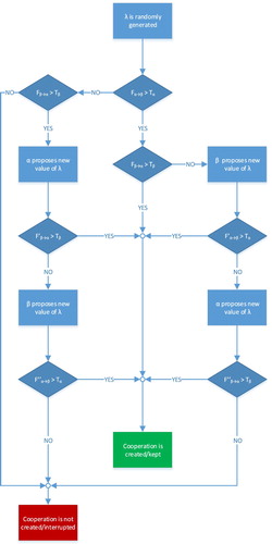
When firms start the negotiation, the value of λ is randomly generated. Both firms compute their fitness value by using Equations 14 and 15. If both fitness values exceed the respective threshold values, the IS relationship is convenient enough for both companies and therefore they start to cooperate. Alternatively, if both fitness values are lower than the respective threshold values, both firms evaluate the IS relationship not convenient enough and therefore they prefer not to cooperate. Accordingly, the IS relationship does not arise. Finally, if F_α→β > T_α and F_β→α ≤ T_β (F_α→β ≤ T_α and F_β→α > T_β) – i.e. the IS relationship is convenient enough for α (β) but not for β (α) – β (α) tries to renegotiate the cost-sharing policy by proposing a new value of λ so that its new fitness value F’_{β→ α} (F’_α→β) results higher than the threshold T_β (T_α). Then, α (β) computes its new fitness value F’_α→β (F’_{β→ α}). If F’_α→β > T_α (F’_{β→ α} > T_β), the IS relationship arises, otherwise α (β) tries in turn to renegotiate the cost-sharing policy by proposing a new value of λ so that the new fitness value F’’_α→β (F’’_β→α) results higher than the threshold T_α (T_β). Then, β (α) computes its new fitness value F’’_β→α (F’’_α→β). If F’’_β→α > T_β (F’’_α→β > T_α), the IS relationship arises, otherwise, the IS relationship is not established. Figure 1 graphically shows the decision-making process.

Figure 1. Flow chart of the agent decision-making process.

This model is tested in a numerical example via computational experiments. In particular, the economic benefits potentially achievable through implementing the IS relationship (see equation 11) are computed for different values of $w^{\alpha }\text{/}{r}^{\beta }$ by adopting the cost–benefit model proposed in Section 3.1. Then, the agent-based model is used to investigate how firms share the additional cooperation costs of IS. Hence, for each considered value of $w^{\alpha }\text{/}{r}^{\beta }$ we can observe: (1) if the IS relationship takes place or not; and (2) the value of λ resulting from the negotiation. To have significant results, the simulation is replicated for 10,000 times. At the end of all replications, for each value of $w^{\alpha }\text{/}{r}^{\beta }$ the following two parameters are computed: (1) the probability that the IS relationship takes place, measured as the ratio between the number of arisen relationships and the total number of replications; and (2) the average value of λ. Thus, it is possible to identify the space of cooperation, which is defined by all the $w^{\alpha }\text{/}{r}^{\beta }$ values allowing IS to rise with a probability higher than zero under a given business scenario characterised by saved and additional costs and individual threshold values. So, the space of cooperation displays the quantity (mis-)match scenarios which have the potential to generate economic benefit for both companies.

4. Numerical example and results

A numerical example is analyzed in this section, aimed at showing how the model operates. This section is divided into two subsections. In the first subsection, the model proposed in Section 3 is applied to a base scenario. In the second subsection, the impact of costs and threshold values on the space of cooperation is investigated via sensitivity analysis. Both subsections are presented together with associated results.

4.1. Base scenario and results

The numerical example concerns the use of marble waste as a substitute of aggregates in the production of concrete (e.g. Hebhoub et al. 2011). Actually, marble residuals are discharged into municipal incinerators or disposed of in landfills, causing high environmental impacts. However, after receiving a treatment process, marble residuals could be used as an alternative aggregate in concrete production.

Suppose that companies α (marble producer) and β (concrete producer) explore the possibility to create a symbiotic relationship. Assume that the technical coefficient of α is W^α = 0.5 – i.e. 0.5 tons of marble residuals are produced per ton of main product – (Hamza, El-Haggar, and Khedr 2011) and the technical coefficient of β is R^β = 0.4 – i.e. 0.4 tons of marble residuals can be used per ton of main product – (Nemati 2015; Pennstate University College of Engineering 2018). As the space of cooperation is assessed with respect to waste supply-demand (mis-)match, we consider x^β as a fixed variable (i.e. 250,000 tons) while x^α is considered as a dynamic variable (i.e. 0–2,000,000 tons). Thus, following equations 1 and 2, the required quantity of primary input β (i.e. $r^{\beta }$) is 100,000 tons and the total quantity of waste α produced by α (i.e. $w^{\alpha }$) varies between 0 and 1,000,000 tons, which means that the $w^{\alpha }/r^{\beta }$ratio ranges between 0 and 10. Furthermore, the values of waste discharge cost, primary input purchase cost, and additional costs to operate industrial symbiosis (IS) in the base scenario are displayed in Table 1.

Table 1. Physical and monetary data of the numerical example.

	Technical coefficients	Data source
$W^{\alpha }$	0.5 tons of waste α/ton of main product α	(Hamza, El-Haggar, and Khedr 2011)
$R^{\beta }$	0.4 tons of primary input β/ton of main product β	(Nemati 2015; Pennstate University College of Engineering 2018)
	Total main outputs
$x^{\alpha }$	0–2,000,000 t of main product α
$x^{\beta }$	250,000 t of main product β
	Total waste production and total primary input requirement
$w^{\alpha }$	0–1,000,000 t of waste α
$r^{\beta }$	100,000 t primary input β
	Unitary cost for base scenario
$C_{w^{\alpha }}^l$	20 €/ton of waste α	(BDA Group 2009)
$C_{r^{\beta }}^s$	100 €/ton primary input β	(Concrete Construction 2018)
$C_{w^{\alpha }}^{\alpha l}$	40 €/ton waste α	(The World Bank 2018)
$C_{r^{\beta }}^{s\beta }$	80 €/ton primary input β	(BDA Group 2009; Dyckerhoff Basal 2018)
$C_{w^{\alpha }{r}^{\beta }}^{\alpha \beta }$	50 €/ton waste α replacing primary input β	(BDA Group 2009; Dyckerhoff Basal 2018)

Furthermore, we assume that each company considers the IS relationship convenient enough if the benefits stemming from the cooperation exceed 20% of non-cooperation costs (i.e. T_α = T_β = 0.2) (Albino, Fraccascia, and Giannoccaro 2016). Here, we compute the total costs in case of non-cooperation (i.e. $C^A$ in equation 5) and cooperation (i.e. $C^B$ in equation 10), the probability that IS arises, and the value of λ as a function of $w^{\alpha }/r^{\beta }$.

Figure 2a shows $C^A$ and $C^B$ as a function of $w^{\alpha }/r^{\beta }$. The IS cooperation is able to create up to 190,000 € of economic benefits. In the best situation, i.e. when $w^{\alpha }/r^{\beta }=1$, these benefits account for 79.2% of non-cooperation costs (if the two companies do not cooperate, $C^A=240,000$€; if they cooperate, $C^B=50,000$€). When $w^{\alpha }/r^{\beta }<1$, the lower $w^{\alpha }/r^{\beta }$, the lower the potential economic benefits are. For instance, when $w^{\alpha }/r^{\beta }=0.5$, ${\mathrm{\Delta }}_{AB}=95,000$€ ($C^A=210,000$€ and $C^B=115,000$), accounting for 45.2% of non-cooperation costs. When $w^{\alpha }/r^{\beta }>1$, the higher$w^{\alpha }/r^{\beta }$, the lower the potential economic benefits compared to the non-cooperation costs. For instance, when $w^{\alpha }/r^{\beta }=2$ the economic benefits account for 63.3% of non-cooperation costs ($C^A=300,000$€) whereas when $w^{\alpha }/r^{\beta }=5$ they account for 39.6% of non-cooperation costs ($C^A=480,000$€).

Figure 2. (a) economic benefit as a function of $w^{\alpha }/r^{\beta }$; (b) average values of the probability of IS implementation and lambda.

Note: The average confidence intervals computed for λ are ±0.00126 (α = 0.05) and ±0.00166 (α = 0.01).

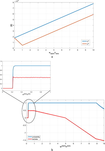
Figure 2b shows the simulation results on the cost-sharing negotiation phase between companies. When $w^{\alpha }/r^{\beta }<0.22$, the probability that firms cooperate is equal to zero. Hence, although the IS relationship could create economic benefits for companies (see Figure 2a), at least one firm is not willing to cooperate because it considers these benefits not enough. The space of cooperation exists for all the values of $w^{\alpha }/r^{\beta }$ ranging from 0.22–10. In particular, when $0.22\le w^{\alpha }/r^{\beta }<0.28$, the probability that firms cooperate is lower than one. In such a range, findings show that 0 < λ < 1, i.e. the additional costs stemming from the IS relationship have to be shared between α and β in order to launch the cooperation. The cooperation arises with a probability equal to one when $0.28\le w^{\alpha }/r^{\beta }<8.92$. However, different values of λ can be observed within this range. In particular, when $0.28\le w^{\alpha }/r^{\beta }\le 1$, λ is approximately equal to 0.5, i.e. firms are available to equally share the additional costs stemming from the IS relationship. When $1<w^{\alpha }/r^{\beta }<4.95$, the higher $w^{\alpha }/r^{\beta }$, the lower the value of λ. This occurs because, whilst β completely resets its input purchase costs, α has to discharge $w^{\alpha }-r^{\beta }$ units of waste in the landfill. Hence, the cooperation arises only if β pays a higher share of additional costs compared to α. When $4.95\le w^{\alpha }/r^{\beta }<8.92$, λ is lower than zero, i.e. the cooperation arises only if β pays all of the additional costs and an extra fee to α. Finally, when $8.92\le w^{\alpha }/r^{\beta }\le 10$, the probability that the cooperation arises is lower than one.

In addition, Figure 2b is useful to explore the operational changes triggered by the fluctuations in $w^{\alpha }/r^{\beta }$. Let us assume that, at the generic time t, $w^{\alpha }/r^{\beta }$ changes from one (perfect match between waste demand and supply) to three, ceteris paribus. This might occur due to several reasons: (1) the amount of waste produced by α is tripled because of an increase in the amount of main output generated ($x_t^{\alpha }=3x_{t-1}^{\alpha }$), ceteris paribus; (2) the amount of wastes required by β is three times lower because of improved technical efficiency of production process of β ($R_t^{\beta }=\left(1/3\right)R_{t-1}^{\beta }$), ceteris paribus; (3) the amount of wastes required by β is three times lower because of the reduction in the amount of main output generated ($x_t^{\beta }=3x_{t-1}^{\beta }$), ceteris paribus; or (4) different combinations of the above-mentioned factors.³ In such a case, the IS relationship would be stable only if companies renegotiate the cost-sharing policy and in particular if β would be available to pay a higher percentage of additional costs. In fact, λ decreases from 0.5–0.25, meaning that now β has to pay 75% of the additional costs compared to 50% it paid when the relationship was created. Otherwise, if β does not accept such a renegotiation, the IS relationship would be interrupted.

4.2. Impact of costs and threshold value on the space of cooperation

In this section, the role of the following parameters influencing the space of cooperation is explored: waste discharge costs of α, input purchase costs of β, additional costs stemming from the IS relationship, and the threshold value. This analysis is useful to investigate the impact of the above-mentioned factors on the emergence of a new IS relationship as well as the extent to which an existing IS relationship is resilient to changes of these factors. First, the impact of changes in waste discharge cost is explained in detail, followed by the representation of the findings of the sensitivity analysis for primary input purchase cost, additional costs of IS, and the threshold value.

Specific to the waste discharge cost, two cases are considered: (1) $C_{w^{\alpha }}^l+C_{w^{\alpha }}^{\alpha l}$ is halved; and (2) $C_{w^{\alpha }}^l+C_{w^{\alpha }}^{\alpha l}$ is doubled.

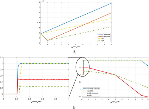
Let us consider that $C_{w^{\alpha }}^l+C_{w^{\alpha }}^{\alpha l}$ is halved. Figure 3a shows the difference between $C^A$ and $C^B$. The results are provided compared to the base case so that we can observe the changes between the two cases. When $w^{\alpha }/r^{\beta }\le 1$, the economic benefits created by the cooperation account for a lower share of non-cooperation costs compared to the base case. On the other hand, when $w^{\alpha }/r^{\beta }>1$, this share increases compared to the base case. Following Figure 3b, the cooperation does not arise when $w^{\alpha }/r^{\beta }<0.25$ (compared to 0.22 in the base case), it can arise with probability ranging between zero and one when $0.25\le w^{\alpha }/r^{\beta }<0.29$ (compared to $0.22\le w^{\alpha }/r^{\beta }<0.28$ in the base case) and it arises with probability equal to one when $0.29\le w^{\alpha }/r^{\beta }\le 10$ (compared to $0.28\le w^{\alpha }/r^{\beta }<8.92$ in the base case). When $0.25\le w^{\alpha }/r^{\beta }\le 4.97$, the value of λ ranges between zero and one and decreases compared to the base case. This means that the cooperation can arise/be kept only if β pays a higher percentage of the additional costs compared to the base case. When $4.97<w^{\alpha }/r^{\beta }\le 10$, the value of λ is lower than zero and is always higher than the corresponding value in the base case. This indicates that α is willing to launch cooperation with less extra payment from β.

Figure 3. (a) economic benefit as a function of $w^{\alpha }/r^{\beta }$ when discharge cost is halved; (b) average values of the probability of IS implementation and lambda when discharge cost is halved.

Note: The average confidence intervals computed for λ are ±0.00077 (α = 0.05) and ±0.00101 (α = 0.01).

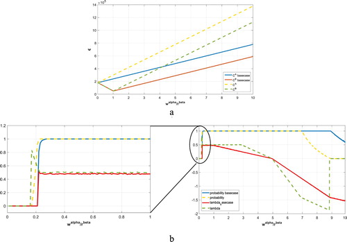
Let us assume that $C_{w^{\alpha }}^l+C_{w^{\alpha }}^{\alpha l}$ is doubled. Figure 4a shows the difference between $C^A$ and $C^B$. When $w^{\alpha }/r^{\beta }\le 1$, the economic benefits thanks to the cooperation account for a higher share of non-cooperation costs compared to the base case. On the other hand, when $w^{\alpha }/r^{\beta }>1$, this share decreases compared to the base case. Following Figure 4b, the cooperation does not arise when $w^{\alpha }/r^{\beta }<0.17$ (compared to 0.22 in the base case), it can arise with probability ranging between zero and one when $0.17\le w^{\alpha }/r^{\beta }<0.22$ (compared to $0.22\le w^{\alpha }/r^{\beta }<0.28$ in the base case), it arises with probability equal to one when $0.22\le w^{\alpha }/r^{\beta }<6.97$ (compared to $0.28\le w^{\alpha }/r^{\beta }<8.92$ in the base case), it can arise with probability between zero and one when $6.97\le w^{\alpha }/r^{\beta }<8.93$, and it does not arise when $8.93\le w^{\alpha }/r^{\beta }\le 10$. When $0.17\le w^{\alpha }/r^{\beta }\le 4.97$, the value of λ ranges between zero and one and increases compared to the base case. Note also that when $w^{\alpha }/r^{\beta }=2.98$, the value of λ starts to decrease while in the base scenario this occurs for a lower ratio, i.e. when$w^{\alpha }/r^{\beta }=1.10$. These mean that the cooperation can arise/be kept only if α pays a higher percentage of the additional costs compared to the base case. This behaviour of α is motivated by the fact that its non-cooperation costs become higher due to the increase in the waste discharge costs. In contrast, when $4.97<w^{\alpha }/r^{\beta }\le 8.93$, the value of λ is lower than zero and it is lower than the corresponding value in the base scenario. This means that α is ready to cooperate only if β pays a higher amount of extra money compared to the base case. This behaviour of α is motivated by the fact that once the ratio $w^{\alpha }/r^{\beta }$ increases, it has more difficulty to keep the IS relationship as its economic benefits from IS decrease compared to its non-cooperation costs.

Figure 4. (a) economic benefit as a function of $w^{\alpha }/r^{\beta }$ when discharge cost is doubled; (b) average values of the probability of IS implementation and lambda when discharge cost is doubled.

Note: The average confidence intervals computed for λ are ±0.00241 (α = 0.05) and ±0.00317 (α = 0.01).

The identical procedure followed in the sensitivity analysis for waste discharge cost is also followed for primary input purchase cost, additional costs of IS, and the threshold value. The associated findings are displayed in Figures 5–10. An overall assessment of the changes in the space of cooperation is summarised in Table 2 and the changes in the values of λ are synoptically reported in Table 3. All these findings are discussed in Section 5.

Figure 5. (a) economic benefit as a function of $w^{\alpha }/r^{\beta }$ when purchase cost is halved; (b) average values of the probability of IS implementation and lambda when purchase cost is halved.

Note: The average confidence intervals computed for λ are ±0.00226 (α = 0.05) and ±0.00297 (α = 0.01).

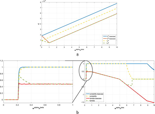
Figure 6. (a) economic benefit as a function of $w^{\alpha }/r^{\beta }$ when purchase cost is doubled; (b) average values of the probability of IS implementation and lambda when purchase cost is doubled.

Note: The average confidence intervals computed for λ are ±0.00159 (α = 0.05) and ±0.00203 (α = 0.01).

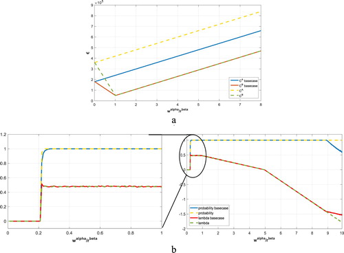
Figure 7. (a) economic benefit as a function of $w^{\alpha }/r^{\beta }$ when additional cost is halved; (b) average values of the probability of IS implementation and lambda when additional cost is halved.

Note: The average confidence intervals computed for λ are ±0.00216 (α = 0.05) and ±0.00284 (α = 0.01).

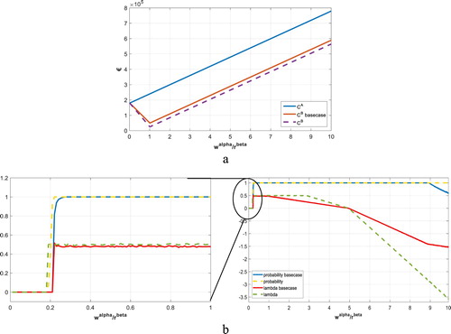
Figure 8. (a) economic benefit as a function of $w^{\alpha }/r^{\beta }$ when additional cost is doubled; (b) average values of the probability of IS implementation and lambda when additional cost is doubled.

Note: The average confidence intervals computed for λ are ±0.00126 (α = 0.05) and ±0.00165 (α = 0.01).

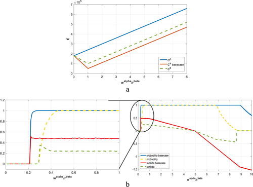
Figure 9. Average values of the probability of IS implementation and lambda when threshold value is halved.

Note: The average confidence intervals computed for λ are ±0.00327 (α = 0.05) and ±0.00432 (α = 0.01).

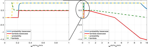
Figure 10. Average values of the probability of IS implementation and lambda when threshold value is doubled.

Note: The average confidence intervals computed for λ are ±0.00372 (α = 0.05) and ±0.00489 (α = 0.01).

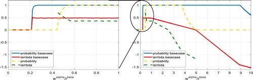
Table 2. Space of cooperation denoted by probability that IS cooperation arises. Green cells: probability equal to 1; Yellow cells: probability between 0 and 1; Red cells: probability equal to 0.

Table 3. Values of λ in all the investigated scenarios (colours of cells) for different values of $w^{\alpha }/r^{\beta }$and comparison with the base case (symbols). Brown cells: 0 ≤ λ < 1, Blue cells: λ < 0; (+) denotes a higher value compared to the base case, (−) denotes a lower value compared to the base case.

5. Discussion

This section is divided into two parts to discuss the findings, implications, and shortcomings of the paper. The first part addresses the role of waste supply-demand quantity match on cost-sharing and on the probability of implementing industrial symbiosis (IS). The second part covers the role of changes in waste discharge cost, primary input purchase cost, additional cooperation cost of IS, and the threshold value on the space of cooperation for companies from the managerial perspective.

5.1. Waste supply-demand quantity match

Following equations 1 and 2, there are two main factors influencing the quantity of waste produced by α (i.e. w^α) and the quantity of primary input used by β (i.e. r^β): (1) the adopted technology, represented by waste production coefficient (i.e. W^α) and primary input requirement coefficient (i.e. R^β); and (2) the total production of main outputs (i.e. x^α and x^β), triggered by their market demands. In the initial stage, companies do not share any common material flows, hence they have no control over the produced and required waste quantities by each other. Accordingly, all computations in our analyses are implemented over the ratio of w^α/r^β. Thus, both companies can assess the initial conditions for quantity match: perfect match (w^α/r^β = 1), waste supply higher than the demand (w^α/r^β > 1), and waste supply lower than the demand (w^α/r^β < 1). In all scenarios, minimum costs are obtained in the perfect match case. However, for companies located in traditionally disengaged sectors, it is hard to foresee in which quantity-matching scenario they might operate the IS without sharing information. In some cases, presence of a waste surplus or presence of a primary input scarcity or abundance can be publicly known. For example, in the Netherlands, there is considerable amount of excess manure, which is the waste of animal-farming sector. Manure discharge is allowed to arable lands as an alternative fertiliser. However, since a publicly-known regulation that limits the amount of manure to be discharged in arable lands is imposed by the government, animal-farmers need to pay arable land owners to provide them with manure (Yazan et al. 2018). Similarly, in a specific geographic area, there might be abundance of a primary input with low purchase cost, which might strongly decrease the chance of IS implementation. Vice versa, the scarcity of a primary in a given geographic area might lower the barriers against IS implementation via replacement of this primary input with a waste. Hence, the quantity match plays a critical role and companies might find themselves anywhere in the Figures 2–10. As observed in Figures 2–10, according to the waste supply-demand quantity match, the probability that IS is implemented and the cost-sharing strategy change.

If the probability of IS implementation is equal to one, then, there is absolutely a space of cooperation for companies, which enables both of them to gain economic benefits. If the probability of IS implementation ranges between zero and one, then there is a space of cooperation for companies, which might allow both of them to gain economic benefits. However, this is not an absolute fact, i.e. cooperation might not be profitable for both companies, depending on the existing and additional costs as well as the threshold values for each company. By applying sensitivity analysis to these costs, it is observed that the space of cooperation might be larger or smaller. Findings show that the lower the waste supply-demand quantity mismatch (i.e. the ratio of w^α/ r^β is closer to one) the higher the probability that IS is profitable for both sides and the cooperation arises. It is also observed that, for very low values of w^α/r^β, the probability that IS arises is equal to zero. This means that a minimum level of waste supply is required to launch the cooperation, which is consistent with previous studies (e.g. Fichtner et al. 2005; Li, Dong, and Ren 2015; Ohnishi et al. 2017). Alternatively, if the supply is much higher than the demand, then the probability of IS implementation decreases from one starting from a certain value of w^α/r^β > 1. Such a probability remains equal to one if waste discharge costs are lower (Figure 3b) or purchase costs are higher (Figure 6b) or additional cooperation costs are lower (Figure 7b) or threshold value is lower (Figure 9) than those of the base scenario. On the other hand, i.e. if waste discharge costs are higher (Figure 4b) or purchase costs are lower (Figure 5b) or additional cooperation costs are higher (Figure 8b) or threshold value is higher (Figure 10) than those of base scenario, the probability that IS arises decreases below one at a lower value of w^α/r^β > 1. Thus, by implementing the model proposed in this paper, companies can be aware of their chances of implementing IS and can adopt business strategies accordingly.

The most relevant question for implementing an efficient business strategy in IS is ‘who pays additional cooperation costs of IS?’. In our model, the cost-sharing is defined by λ, the parameter decisive for the monetary flows. λ fluctuates for all scenarios when w^α/r^β changes. In particular, it is observed that, depending on the quantity ratio, one company might have the disadvantage of paying (part of) the additional cooperation costs or even paying extra to the other company to send (receive) waste to (from) it. However, if the probability of implementing IS is equal to one, there is economic convenience for both parties even in such cases. This means that, in the absence of a mature waste market, ‘who pays what’ is a matter of operational conditions that might change the willingness-to-cooperate and bargaining power of companies (Yazan, Clancy, and Lovett 2012). For example, Yazan et al. (2018) study an IS case between animal farmers and biogas producers in Overijssel (East Netherlands) based on the use of animal manure for biogas production. Their findings show that economically convenient IS is possible between two actor types in a price range of −3.33 €/ton manure (animal farmers pay to biogas producers) and 7.03 €/ton manure (biogas producers pay to animal farmers). Hence, implementing IS is possible via either paying to or being paid by the IS partner. In fact, the numerical example analyzed in this paper shows similar results with the fluctuating values of λ.

From the business-making perspective, the findings of this paper are highly relevant because IS generally suffers from the lack of information (e.g. Sakr et al. 2011; Golev, Corder, and Giurco 2015; Aid et al. 2017), which leads to the challenge of foreseeing future benefits of IS in a limited way. If companies are able to frame the business conditions and accordingly run a decision-making process, then they would be able to develop their business strategies. For example, an online platform that collects and provides companies with technological, demand-related, and economic data can have the function of decision support for companies and play a key role in reducing supply-demand mismatch (Fraccascia and Yazan 2018).

A final observation on the waste supply-demand quantity match concerns the role of technology and market demand for main products. Technological innovations might lead to several consequences for both waste producers and waste receivers. Waste producers might increase the efficiency of the adopted technology via implementing production systems that produce lower amounts of waste per unit of output (the waste coefficient W^α is reduced). Accordingly, w^α will be reduced. Similarly, waste receivers might implement more efficient technologies that consume lower amounts of primary input per unit of output (the input coefficient R^β is reduced). Accordingly, r^β will be reduced. In both cases, the ratio of w^α/r^β fluctuates, thereby changing business conditions and business strategies of companies.

The market demands for companies’ main products play a critical role in IS implementation as the wastes are not produced upon demand but emerge as secondary outputs of main production activities. This nature of waste production renders waste supply-demand quantity match harder to achieve. In particular, the market demand for main product of one company could be high in a specific period while the sales of the other company might be low in the same period, leading to the mismatch between waste supply and demand. Hence, seasonality matters in IS and, apart from influencing the business strategy, seasonality-related situations might cause missed opportunities for IS. Obviously, in such cases companies might look for further cooperators to mitigate the impacts of quantity mismatch on their businesses. This is a matter of emergence of IS networks (ISNs), which remains out of the scope of this paper. Readers interested in the emergence of ISNs are referred, e.g. to Chertow and Ehrenfeld (2012), Doménech and Davies (2011), Bacudio et al. (2016), Ashton, Chopra, and Kashyap (2017), Tudor, Adam, and Bates (2007), Albino, Fraccascia, and Giannoccaro (2016), Fraccascia and Yazan (2018), Tao et al. (2019).

5.2. Waste discharge, primary input purchase, additional cooperation costs, and threshold value

This paper investigates the dynamics of IS, which is a form of circular economic business model (e.g. Bocken et al. 2014; Lüdeke-Freund, Gold, and Bocken 2018; Lüdeke-Freund et al. 2018). In the transition from linear to circular economic business models, we recommend companies to take into account the evolving dynamics of IS. However, the existing business conditions of linear economy play a non-negligible role in such a transition. Indeed, the waste discharge costs, primary input purchase costs, and additional costs of cooperation are shaped by linear business model dynamics and influence the space of cooperation for companies.

The cost of waste discharge might depend on a range of factors: the size of the discharge area, existing regulations for discharge, landfill taxes imposed by governments, weather conditions affecting the humidity of wastes, the distance between waste discharging company and discharge area, city/region/country where the discharge is located, etc. Similarly, the cost of primary input purchase might depend on several factors: the market price and its fluctuations over time, the abundance/scarcity of primary input in a specific region, the distance between purchasing company and the traditional supplier, etc. Finally, the additional cost of cooperation might also vary according to the efforts of companies to search for and to implement IS, the necessity to treat the waste, the costs stemming from waste quality issues, the need for transporting the waste, etc. Threshold value also impacts on the space of cooperation as it might change over time shaped by real-time needs of companies. As companies are autonomous entities in the business environment, each of them has different and dynamic expectations from new businesses.

The above-mentioned potential changes in costs would strongly influence the space of cooperation for companies, as observed in the findings of sensitivity analysis. In fact, if the values of these costs are different, then the probability of implementing IS and the company strategy for cost-sharing changes. Accordingly, companies might find themselves in different scenarios shaped by different cost combinations such as high waste discharge cost and low primary input purchase cost, low waste discharge cost and high primary input purchase cost, etc. Although in our numerical example discharge costs are lower than primary input purchase costs, the generalizability of the proposed model is valid for all types of combinations. For example, if the primary input purchase cost is much higher than the waste discharge cost (which is an unlikely case but among the possibilities), then the cost-sharing parameter as well as the probability of implementing IS would be different than those of numerical example presented in this paper. Indeed, by applying sensitivity analysis to the costs, we observe changes in space of cooperation and business strategies (see Figures 3–10). Therefore, the proposed integration of Enterprise Input-Output (EIO) model and Agent-based modelling (ABM) in this paper is appropriate for the dynamic and case-specific nature of IS and generalisable for one-to-one IS implementation over one waste.

Finally, the waste-primary input substitution is assumed to be one-for-one unit, which would not affect the calculations path if it was different. In cases where one unit of waste does not substitute one unit of primary input, then a simple substitution coefficient can be integrated into the computations (see e.g. Fraccascia and Yazan 2018).

6. Conclusions

This paper provides an operational perspective to business strategy development in industrial symbiosis (IS) relations taking into account the dynamics of IS-based businesses. Practical and managerial contributions can be divided in one-to-one business-making level and production network level.

At the one-to-one level, companies need to cooperate between each other to create value-added from IS. However, waste management induces not only value-added (e.g. profit, green jobs) and cost savings (e.g. waste discharge cost, primary input purchase cost) but also new costs to be dealt with (e.g. waste recycling and transportation cost). In addition, uncertainties on demand and waste quantities cause uncertainties on economic benefits. These problems raise the questions: ‘who will pay for what?’; ‘who will perform which task?’; and ‘who will get how much benefit?’. Such a complexity is the main reason that the waste markets are still underdeveloped, pushing companies to fall into contradictions and miss attractive cooperation opportunities as well as the chance to enhance their environmental performance. This paper fills such a managerial and practical gap by proposing a decision-support model for companies so that they are able to profile their situation and develop cooperation strategies during the run of real-time negotiations. The benefit-sharing schemes should also be analyzed in further research, particularly from supply chain design and contracting perspectives. This is critical to vitalise the theoretical implications of this study in practice.

At the production network level, in promising cases, companies may try to approach to waste streams instead of primary input reserves while implementing a production unit or designing a production network/industrial cluster. Companies may even produce higher amounts of main outputs than the market demand to satisfy the waste demand of another company. Then, cooperation becomes more critical particularly in collaborative demand forecasting, trust-development, and design issues. These would affect the structure of future production networks, which should be approached from a multi-stakeholder perspective, as they would operate with untraditional business dynamics.

In terms of policy contributions, findings show that some potential IS cases are probabilistically less achievable and this problem can be mitigated via governmental regulations, such as landfill taxes or subsidies for recycled waste reuse, etc. (Dong et al. 2013; Fraccascia, Giannoccaro, and Albino 2017a). Thus, governments can support environmentally promising but economically challenging IS cases. For example, the marginal environmental contribution of each company can be taken as a reference point for incentivizing companies. This can be investigated as future research.

In terms of methodological contribution, the integration of Enterprise Input-Output (EIO) model with the Agent-based Modelling (ABM) results in highly satisfactory outcomes. In fact, EIO is an appropriate tool for technological and physical modelling while ABM is suitable to develop business strategies based on ‘what-if’ analysis in real-time. Therefore, the paper is methodologically innovative in terms of combining these approaches, which could further be used in developing research on ‘contracts in IS’. Indeed, the agent-based model proposed in the paper is applicable to all IS cases in which a waste substitutes a primary input, i.e. it is a generalisable decision-support model for IS cases based on waste-to-primary input substitution. The marble-concrete IS represented by the numerical case in this paper is only a demonstration of the model's applicability.

This paper addresses an important gap in IS research, i.e. business development in IS from the operational perspective. It is clear from the numerical example that companies need each other to create added value and they should be fair against each other when they are sharing this value-added. If companies tend to maximize their profits without considering the needs of their potential IS partners, then the risk of falling apart in IS networks is high. Therefore, the theoretical contribution of this paper is the concept of space of cooperation, i.e. the business-making area in which companies should reach an agreement to achieve IS. In future research, authors aim at analyzing the collective behaviour of companies in industrial symbiosis networks (ISNs) about cost-sharing, in order to understand whether developed business strategies converge into a specific type of behaviour, such as fair or opportunistic cost-sharing, coalition forming to gain bargaining power, etc. Finally, future research should also address the strategies to reduce additional costs of IS, which is for example achievable via implementing online information-sharing platforms.

Acknowledgements

This research is funded by European Union’s Horizon 2020 program under grant agreement No. 680843. We would like to thank the two anonymous Reviewers whose comments contributed to improve the quality of the paper.

Disclosure statement

No potential conflict of interest was reported by the authors.

ORCID

Devrim Murat Yazan http://orcid.org/0000-0002-4341-2529

Luca Fraccascia http://orcid.org/0000-0002-6841-9823

Additional information

Funding

This research is funded by European Union’s Horizon 2020 program under grant agreement No. 680843.

Notes

1 Here the reader can read in parallel the role of waste users in the main sentence and the role of waste producers by following parentheses.

2 In fact, based on Equations 12 and 13, it results: ${\mathrm{\Delta }}_{\alpha }+{\mathrm{\Delta }}_{\beta }=\left\{\begin{array}{l}\begin{array}{l}\left[\left(C_{w^{\alpha }}^l+C_{w^{\alpha }}^{\alpha l}\right)\cdot w^{\alpha }-\lambda \cdot C_{w^{\alpha }{r}^{\beta }}^{\alpha \beta }\cdot w^{\alpha }\right]+\left[\left(C_{r^{\beta }}^s+C_{r^{\beta }}^{s\beta }\right)\cdot w^{\alpha }-(1-\lambda )\cdot C_{w^{\alpha }{r}^{\beta }}^{\alpha \beta }\cdot w^{\alpha }\right]\\ =\left[\left(C_{w^{\alpha }}^l+C_{w^{\alpha }}^{\alpha l}\right)+\left(C_{r^{\beta }}^s+C_{r^{\beta }}^{s\beta }\right)-C_{w^{\alpha }{r}^{\beta }}^{\alpha \beta }\right]\cdot w^{\alpha }={\mathrm{\Delta }}_{AB}\text{if}{\text{w}}^{\alpha }\le {\text{r}}^{\beta }\end{array}\\ \begin{array}{l}\left[\left(C_{w^{\alpha }}^l+C_{w^{\alpha }}^{\alpha l}\right)\cdot r^{\beta }-\lambda \cdot C_{w^{\alpha }{r}^{\beta }}^{\alpha \beta }\cdot r^{\beta }\right]+\left[\left(C_{r^{\beta }}^s+C_{r^{\beta }}^{s\beta }\right)\cdot r^{\beta }-(1-\lambda )\cdot C_{w^{\alpha }{r}^{\beta }}^{\alpha \beta }\cdot r^{\beta }\right]\\ =\left[\left(C_{w^{\alpha }}^l+C_{w^{\alpha }}^{\alpha l}\right)+\left(C_{r^{\beta }}^s+C_{r^{\beta }}^{s\beta }\right)-C_{w^{\alpha }{r}^{\beta }}^{\alpha \beta }\right]\cdot r^{\beta }={\mathrm{\Delta }}_{AB}\text{if}{\text{w}}^{\alpha }\ge {\text{r}}^{\beta }\end{array}\end{array}\right.$

3 From the mathematical perspective, $w^{\alpha }/r^{\beta }$could increase also because of higher values of $W^{\alpha }$. However, this is a not realistic assumption. In fact, higher value of $W^{\alpha }$would stand against technological innovation.

References

- Abreu, Mônica Cavalcanti Sá de, and Domenico Ceglia. 2018. “On the Implementation of a Circular Economy: The Role of Institutional Capacity-Building through Industrial Symbiosis.” Resources, Conservation and Recycling 138 (November). Elsevier: 99–109. doi:10.1016/J.RESCONREC.2018.07.001.
- Aid, Graham, Mats Eklund, Stefan Anderberg, and Leenard Baas. 2017. “Expanding Roles for the Swedish Waste Management Sector in Inter-Organizational Resource Management.” Resources, Conservation and Recycling 124: 85–97. doi:10.1016/j.resconrec.2017.04.007.
- Albino, Vito, Erik Dietzenbacher, and Silvana Kühtz. 2003. “Analysing Materials and Energy Flows in an Industrial District Using an Enterprise Input–Output Model.” Economic Systems Research 15 (4): 457–480. doi:10.1080/0953531032000152326.
- Albino, Vito, Luca Fraccascia, and Ilaria Giannoccaro. 2016. “Exploring the Role of Contracts to Support the Emergence of Self-Organized Industrial Symbiosis Networks: An Agent-Based Simulation Study.” Journal of Cleaner Production 112 (January). Elsevier: 4353–4366. doi:10.1016/J.JCLEPRO.2015.06.070.
- Ashton, Weslynne S. 2011. “Managing Performance Expectations of Industrial Symbiosis.” Business Strategy and the Environment 20 (5). Wiley-Blackwell: 297–309. doi:10.1002/bse.696.
- Ashton, Weslynne S., Shauhrat S. Chopra, and Rahul Kashyap. 2017. “Life and Death of Industrial Ecosystems.” Sustainability 9 (4). Multidisciplinary Digital Publishing Institute: 605. doi:10.3390/su9040605.
- Axelrod, Robert. 1997. The Complexity of Cooperation: Agent-Based Models of Competition and Collaboration. Princeton, NJ: Princeton University Press.
- Bacudio, Lindley R., Michael Francis D. Benjamin, Ramon Christian P. Eusebio, Sed Anderson K. Holaysan, Michael Angelo B. Promentilla, Krista Danielle S. Yu, and Kathleen B. Aviso. 2016. “Analyzing Barriers to Implementing Industrial Symbiosis Networks Using DEMATEL.” Sustainable Production and Consumption 7: 57–65. doi:10.1016/j.spc.2016.03.001.
- Batten, David F. 2009. “Fostering Industrial Symbiosis with Agent-Based Simulation and Participatory Modeling.” Journal of Industrial Ecology 13 (2). Blackwell Publishing Inc: 197–213. doi:10.1111/j.1530-9290.2009.00115.x.
- BDA Group. 2009. The Full Cost of Landfill Disposal in Australia. http://www.environment.gov.au/system/files/resources/2e935b70-a32c-48ca-a0ee-2aa1a19286f5/files/landfill-cost.pdf.
- Benjamin, Michael Francis D., Raymond R. Tan, and Luis F. Razon. 2015. “Probabilistic Multi-Disruption Risk Analysis in Bioenergy Parks via Physical Input-Output Modeling and Analytic Hierarchy Process.” Sustainable Production and Consumption 1 (January). Elsevier: 22–33. doi:10.1016/j.spc.2015.05.001.
- Bichraoui, N., B. Guillaume, and A. Halog. 2013. “Agent-Based Modelling Simulation for the Development of an Industrial Symbiosis - Preliminary Results.” Procedia Environmental Sciences 17 (January). Elsevier: 195–204. doi:10.1016/J.PROENV.2013.02.029.
- Bocken, N. M. P., S. W. Short, P. Rana, and S. Evans. 2014. “A Literature and Practice Review to Develop Sustainable Business Model Archetypes.” Journal of Cleaner Production 65 (February): 42–56. doi:10.1016/j.jclepro.2013.11.039.
- Bonabeau, Eric. 2002. “Agent-Based Modeling: Methods and Techniques for Simulating Human Systems.” Proceedings of the National Academy of Sciences 99 (May). National Academy of Sciences: 7280–7287. doi:10.1073/pnas.082080899.
- Cao, Kai, Xiao Feng, and Hui Wan. 2009. “Applying Agent-Based Modeling to the Evolution of Eco-Industrial Systems.” Ecological Economics 68 (11): 2868–2876. doi:10.1016/j.ecolecon.2009.06.009.
- Carley, K. M., and L. Gasser. 1999. “Computational Organization Theory.” In Multiagent Systems: A Modern Approach to Distributed Artificial Intelligence, edited by G. Weiss, 299–330. Cambridge, MA: The MIT Press. https://books.google.it/books?hl=it&lr=&id=JYcznFCN3xcC&oi=fnd&pg=PA299&dq=Computational+organization+theory&ots=IH5ZrALk_s&sig=7nr0Vv74oIN3YdGPuXInUdCr9jE&redir_esc=y#v=onepage&q=Computational organization theory&f=false.
- Chan, F. T. S. 2003. “Interactive Selection Model for Supplier Selection Process: An Analytical Hierarchy Process Approach.” International Journal of Production Research 41 (15): 3549–3579. doi:10.1080/0020754031000138358.
- Chertow, Marian R. 2000. “Industrial Symbiosis: Literature and Taxonomy.” Annual Review of Energy and the Environment 25 (1): 313–337. doi:10.1002/(SICI)1099-0526(199711/12)3:2<16::AID-CPLX4>3.0.CO;2-K.
- Chertow, Marian R., and John Ehrenfeld. 2012. “Organizing Self-Organizing Systems.” Journal of Industrial Ecology 16 (1). Wiley/Blackwell (10.1111): 13–27. doi:10.1111/j.1530-9290.2011.00450.x.
- Chopra, Shauhrat S., and Vikas Khanna. 2014. “Understanding Resilience in Industrial Symbiosis Networks: Insights from Network Analysis.” Journal of Environmental Management 141 (August). Academic Press: 86–94. doi:10.1016/J.JENVMAN.2013.12.038.
- Concrete Construction. 2018. What You Should Know about Aggregates. https://www.concreteconstruction.net/_view-object?id=00000153-8b5a-dbf3-a177-9f7b16080000.
- Costa, Inês, and Paulo Ferrão. 2010. “A Case Study of Industrial Symbiosis Development Using a Middle-out Approach.” Journal of Cleaner Production 18 (10): 984–992. doi:10.1016/j.jclepro.2010.03.007.
- Cutaia, Laura, Roberto Morabito, Grazia Barberio, Erika Mancuso, Claudia Brunori, Pasquale Spezzano, Antonio Mione, Camillo Mungiguerra, Ornella Li Rosi, and Francesco Cappello. 2014. “The Project for the Implementation of the Industrial Symbiosis Platform in Sicily: The Progress After the First Year of Operation.” In Pathways to Environmental Sustainability: Methodologies and Experiences, edited by Roberta Salomone, and Giuseppe Saija, 205–214. Cham: Springer International Publishing. doi:10.1007/978-3-319-03826-1_20.
- Domenech, Teresa, Raimund Bleischwitz, Asel Doranova, Dimitris Panayotopoulos, and Laura Roman. 2019. “Mapping Industrial Symbiosis Development in Europe_ Typologies of Networks, Characteristics, Performance and Contribution to the Circular Economy.” Resources, Conservation and Recycling 141 (February). Elsevier: 76–98. doi:10.1016/J.RESCONREC.2018.09.016.
- Doménech, Teresa, and Michael Davies. 2011. “The Role of Embeddedness in Industrial Symbiosis Networks: Phases in the Evolution of Industrial Symbiosis Networks.” Business Strategy and the Environment 20 (5). Wiley-Blackwell: 281–296. doi:10.1002/bse.695.
- Dong, Liang, Hui Zhang, Tsuyoshi Fujita, Satoshi Ohnishi, Huiquan Li, Minoru Fujii, and Huijuan Dong. 2013. “Environmental and Economic Gains of Industrial Symbiosis for Chinese Iron/Steel Industry: Kawasaki’s Experience and Practice in Liuzhou and Jinan.” Journal of Cleaner Production 59 (November). Elsevier: 226–238. doi:10.1016/J.JCLEPRO.2013.06.048.
- Dyckerhoff Basal. 2018. A Unique Method of Transporting Aggregates: Safer, Cheaper, and More Sustainable. http://www.dyckerhoff-basal.com/online/download.jsp?idDocument=9&instance=1.
- Epstein, J. M., and R. Axtell. 1996. Growing Artificial Societies: Social Science from the Bottom Up. Washington, DC: Brooking Institution Press.
- Esty, Daniel C, and Michael E Porter. 1998. “Industrial Ecology and Competitiveness.” Journal of Industrial Ecology 2 (1): 35–43. doi:10.1162/jiec.1998.2.1.35.
- European Commission. 2015. Closing the Loop - An EU Action Plan for the Circular Economy. COM. Bruxelles. http://eur-lex.europa.eu/legal-content/EN/TXT/?uri=CELEX%3A52015DC0614.
- Fichtner, Wolf, Ingela Tietze-Stöckinger, Michael Frank, and Otto Rentz. 2005. “Barriers of Interorganisational Environmental Management: Two Case Studies on Industrial Symbiosis.” Progress in Industrial Ecology, an International Journal 2 (1): 73–88. doi:10.1504/PIE.2005.006778.
- Fraccascia, Luca, Vito Albino, and Claudio A. Garavelli. 2017. “Technical Efficiency Measures of Industrial Symbiosis Networks Using Enterprise Input-Output Analysis.” International Journal of Production Economics 183: 273–286. doi:10.1016/j.ijpe.2016.11.003.
- Fraccascia, Luca, Ilaria Giannoccaro, and Vito Albino. 2017a. “Efficacy of Landfill Tax and Subsidy Policies for the Emergence of Industrial Symbiosis Networks: An Agent-Based Simulation Study.” Sustainability 9 (4). Multidisciplinary Digital Publishing Institute: 521. doi:10.3390/su9040521.
- Fraccascia, Luca, Ilaria Giannoccaro, and Vito Albino. 2017b. “Rethinking Resilience in Industrial Symbiosis: Conceptualization and Measurements.” Ecological Economics 137 (July). Elsevier: 148–162. doi:10.1016/J.ECOLECON.2017.02.026.
- Fraccascia, Luca, and Devrim Murat Yazan. 2018. “The Role of Online Information-Sharing Platforms on the Performance of Industrial Symbiosis Networks.” Resources, Conservation and Recycling 136 (September). Elsevier: 473–485. doi:10.1016/J.RESCONREC.2018.03.009.
- Ghali, Mohamed Raouf, Jean-Marc Frayret, and Chahid Ahabchane. 2017. “Agent-Based Model of Self-Organized Industrial Symbiosis.” Journal of Cleaner Production 161 (September). Elsevier: 452–465. doi:10.1016/J.JCLEPRO.2017.05.128.
- Ghodsypour, S. H., and C. O’Brien. 1998. “A Decision Support System for Supplier Selection Using an Integrated Analytic Hierarchy Process and Linear Programming.” International Journal of Production Economics 56–57 (September). Elsevier: 199–212. doi:10.1016/S0925-5273(97)00009-1.
- Ghodsypour, S. H., and C. O’Brien. 2001. “The Total Cost of Logistics in Supplier Selection, under Conditions of Multiple Sourcing, Multiple Criteria and Capacity Constraint.” International Journal of Production Economics 73 (1). Elsevier: 15–27. doi:10.1016/S0925-5273(01)00093-7.
- Giannoccaro, Ilaria. 2015. “Adaptive Supply Chains in Industrial Districts: A Complexity Science Approach Focused on Learning.” International Journal of Production Economics 170: 576–589. doi:10.1016/j.ijpe.2015.01.004.
- Giannoccaro, Ilaria, Anand Nair, and Thomas Choi. 2018. “The Impact of Control and Complexity on Supply Network Performance: An Empirically Informed Investigation Using NK Simulation Analysis.” Decision Sciences 49 (4). John Wiley & Sons, Ltd (10.1111): 625–659. doi:10.1111/deci.12293.
- Goldstein, Jeffrey. 1999. “Emergence as a Construct: History and Issues.” Emergence 1 (1). Lawrence Erlbaum Associates, Inc.: 49–72. doi:10.1207/s15327000em0101_4.
- Golev, Artem, Glen D. Corder, and Damien P. Giurco. 2015. “Barriers to Industrial Symbiosis: Insights from the Use of a Maturity Grid.” Journal of Industrial Ecology 19 (1): 141–153. doi:10.1111/jiec.12159.
- Govindan, Kannan, and Mia Hasanagic. 2018. “A Systematic Review on Drivers, Barriers, and Practices towards Circular Economy: A Supply Chain Perspective.” International Journal of Production Research 56 (1–2). Taylor & Francis: 278–311. doi:10.1080/00207543.2017.1402141.
- Govindan, Kannan, P. C. Jha, and Kiran Garg. 2016. “Product Recovery Optimization in Closed-Loop Supply Chain to Improve Sustainability in Manufacturing.” International Journal of Production Research 54 (5). Taylor & Francis: 1463–1486. doi:10.1080/00207543.2015.1083625.
- Grubbstrom, Robert W, and Ou Tang. 2000. “An Overview of Input-Output Analysis Applied to Production-Inventory Systems.” Economic Systems Research 12 (1): 3–25. doi:10.1080/095353100111254.
- Hamza, Rania A, Salah El-Haggar, and Safwan Khedr. 2011. “Marble and Granite Waste: Characterization and Utilization in Concrete Bricks.” International Journal of Bioscience, Biochemistry and Bioinformatics 1 (4): 286–291.
- Hebhoub, H., H. Aoun, M. Belachia, H. Houari, and E. Ghorbel. 2011. “Use of Waste Marble Aggregates in Concrete.” Construction and Building Materials 25 (3). Elsevier: 1167–1171. doi:10.1016/J.CONBUILDMAT.2010.09.037.
- Hill, Roger M. 1999. “The Optimal Production and Shipment Policy for the Single-Vendor Singlebuyer Integrated Production-Inventory Problem.” International Journal of Production Research 37 (11): 2463–2475. doi:10.1080/002075499190617.
- Holland, John H. 2002. “Complex Adaptive Systems and Spontaneous Emergence.” In Complexity and Industrial Clusters, edited by A. Quadro Curzio, and M. Fortis, 25–34. Heidelberg: Physica-Verlag HD. doi:10.1007/978-3-642-50007-7_3.
- Jacobsen, Noel Brings. 2006. “Industrial Symbiosis in Kalundborg, Denmark: A Quantitative Assessment of Economic and Environmental Aspects.” Journal of Industrial Ecology 10 (1–2): 239–255. doi:10.1162/108819806775545411.
- Kim, Hyeong-Woo, Satoshi Ohnishi, Minoru Fujii, Tsuyoshi Fujita, and Hung-Suck Park. 2018. “Evaluation and Allocation of Greenhouse Gas Reductions in Industrial Symbiosis.” Journal of Industrial Ecology 22 (2). John Wiley & Sons, Ltd (10.1111): 275–287. doi:10.1111/jiec.12539.
- Kuhtz, Silvana, Chaoying Zhou, Vito Albino, and Devrim M. Yazan. 2010. “Energy Use in Two Italian and Chinese Tile Manufacturers: A Comparison Using an Enterprise Input–Output Model.” Energy 35 (1): 364–374. doi:10.1016/j.energy.2009.10.002.
- Kumar, Sameer, Steve Teichman, and Tobias Timpernagel. 2012. “A Green Supply Chain Is a Requirement for Profitability.” International Journal of Production Research. Taylor & Francis Group. doi:10.1080/00207543.2011.571924.
- Li, Hong, Liang Dong, and Jingzheng Ren. 2015. “Industrial Symbiosis as a Countermeasure for Resource Dependent City: A Case Study of Guiyang, China.” Journal of Cleaner Production 107 (November). Elsevier: 252–266. doi:10.1016/J.JCLEPRO.2015.04.089.
- Liang, Sai, Xiao-Ping Jia, and Tian-Zhu Zhang. 2011. “Three-Dimensional Hybrid Enterprise Input–Output Model for Material Metabolism Analysis: A Case Study of Coal Mines in China.” Clean Technologies and Environmental Policy 13 (1). Springer-Verlag: 71–85. doi:10.1007/s10098-010-0282-8.
- Lin, Xiannuan, and Karen R. Polenske. 1998. “Input—Output Modeling of Production Processes for Business Management.” Structural Change and Economic Dynamics 9 (2). North-Holland: 205–226. doi:10.1016/S0954-349X(97)00034-9.
- Lombardi, D. Rachel, and Peter Laybourn. 2012. “Redefining Industrial Symbiosis.” Journal of Industrial Ecology 16 (1): 28–37. doi:10.1111/j.1530-9290.2011.00444.x.
- Low, Jonathan Sze Choong, Tobias Bestari Tjandra, Fajrian Yunus, Si Ying Chung, Daren Zong Loong Tan, Benjamin Raabe, Ng Yen Ting, et al. 2018. “A Collaboration Platform for Enabling Industrial Symbiosis: Application of the Database Engine for Waste-to-Resource Matching.” Procedia CIRP 69 (January). Elsevier: 849–854. doi:10.1016/J.PROCIR.2017.11.075.
- Lüdeke-Freund, Florian, Sarah Carroux, Alexandre Joyce, Lorenzo Massa, and Henning Breuer. 2018. “The Sustainable Business Model Pattern Taxonomy—45 Patterns to Support Sustainability-Oriented Business Model Innovation.” Sustainable Production and Consumption 15 (July). Elsevier: 145–162. doi:10.1016/J.SPC.2018.06.004.
- Lüdeke-Freund, Florian, Stefan Gold, and Nancy M.P. Bocken. 2018. “A Review and Typology of Circular Economy Business Model Patterns.” Journal of Industrial Ecology, April 25. doi:10.1111/jiec.12763.
- Lyons, Donald. 2007. “A Spatial Analysis of Loop Closing Among Recycling, Remanufacturing, and Waste Treatment Firms in Texas.” Journal of Industrial Ecology 11 (1): 43–54. doi:10.1162/jiec.2007.1029.
- Maqbool, Amtul, Francisco Mendez Alva, and Greet Van Eetvelde. 2018. “An Assessment of European Information Technology Tools to Support Industrial Symbiosis.” Sustainability 11 (1). Multidisciplinary Digital Publishing Institute: 131. doi:10.3390/su11010131.
- Martin, Michael, Niclas Svensson, and Mats Eklund. 2015. “Who Gets the Benefits? An Approach for Assessing the Environmental Performance of Industrial Symbiosis.” Journal of Cleaner Production 98: 263–271. doi:10.1016/j.jclepro.2013.06.024.
- Mathiyazhagan, K., Kannan Govindan, and A. Noorul Haq. 2014. “Pressure Analysis for Green Supply Chain Management Implementation in Indian Industries Using Analytic Hierarchy Process.” International Journal of Production Research 52 (1). Taylor & Francis: 188–202. doi:10.1080/00207543.2013.831190.
- Mattila, Tuomas J, Suvi Pakarinen, and Laura Sokka. 2010. “Quantifying the Total Environmental Impacts of an Industrial Symbiosis - A Comparison of Process-, Hybrid and Input - Output Life Cycle Assessment.” Environmental Science and Technology 44: 4309–4314.
- Mirata, Murat. 2004. “Experiences from Early Stages of a National Industrial Symbiosis Programme in the UK: Determinants and Coordination Challenges.” Journal of Cleaner Production 12 (8–10): 967–983. doi:10.1016/j.jclepro.2004.02.031.
- Murray, Alan, Keith Skene, and Kathryn Haynes. 2017. “The Circular Economy: An Interdisciplinary Exploration of the Concept and Application in a Global Context.” Journal of Business Ethics 140 (3). Springer Netherlands: 369–380. doi:10.1007/s10551-015-2693-2.
- Nemati, Kamran. 2015. Aggregates for Concrete. http://courses.washington.edu/cm425/aggregate.pdf.
- Ohnishi, Satoshi, Huijuan Dong, Yong Geng, Minoru Fujii, and Tsuyoshi Fujita. 2017. “A Comprehensive Evaluation on Industrial & Urban Symbiosis by Combining MFA, Carbon Footprint and Emergy Methods—Case of Kawasaki, Japan.” Ecological Indicators 73. Elsevier Ltd: 513–524. doi:10.1016/j.ecolind.2016.10.016.
- Pennstate University College of Engineering. 2018. The Effect of Aggregate Properties on Concrete. https://www.engr.psu.edu/ce/courses/ce584/concrete/library/materials/aggregate/aggregatesmain.htm.
- Romero, Elena, and M. Carmen Ruiz. 2014. “Proposal of an Agent-Based Analytical Model to Convert Industrial Areas in Industrial Eco-Systems.” Science of the Total Environment 468–469 (January): 394–405. doi:10.1016/j.scitotenv.2013.08.049.
- Saavedra, Yovana M.B., Diego R. Iritani, Ana L.R. Pavan, and Aldo R. Ometto. 2018. “Theoretical Contribution of Industrial Ecology to Circular Economy.” Journal of Cleaner Production 170 (January). Elsevier: 1514–1522. doi:10.1016/J.JCLEPRO.2017.09.260.
- Sabri, Ehap H., and Benita M. Beamon. 2000. “A Multi-Objective Approach to Simultaneous Strategic and Operational Planning in Supply Chain Design.” Omega 28 (5): 581–598. doi:10.1016/S0305-0483(99)00080-8.
- Sakr, D., L. Baas, S. El-Haggar, and D. Huisingh. 2011. “Critical Success and Limiting Factors for Eco-Industrial Parks: Global Trends and Egyptian Context.” Journal of Cleaner Production 19 (11). Elsevier: 1158–1169. doi:10.1016/J.JCLEPRO.2011.01.001.
- Sarkis, Joseph, and Qingyun Zhu. 2018. “Environmental Sustainability and Production: Taking the Road Less Travelled.” International Journal of Production Research 56 (1–2). Taylor & Francis: 743–759. doi:10.1080/00207543.2017.1365182.
- Sonis, Michael, and Geoffrey J D Hewings. 2007. Coefficient Change and Innovation Spread in Input-Output Models. http://www.ufjf.br/poseconomia/files/2010/01/td_004_2007.pdf.
- Tan, R. R., K. B. Aviso, C. D. Cayamanda, A. S. F. Chiu, M. A. B. Promentilla, A. T. Ubando, and K. D. S. Yu. 2016. “A Fuzzy Linear Programming Enterprise Input–Output Model for Optimal Crisis Operations in Industrial Complexes.” International Journal of Production Economics 181: 410–418. doi:10.1016/j.ijpe.2015.10.012.
- Tao, Yuan, Steve Evans, Zongguo Wen, and Mingfeng Ma. 2019. “The Influence of Policy on Industrial Symbiosis from the Firm’s Perspective: A Framework.” Journal of Cleaner Production 213 (March). Elsevier: 1172–1187. doi:10.1016/J.JCLEPRO.2018.12.176.
- Tudor, Terry, Emma Adam, and Margaret Bates. 2007. “Drivers and Limitations for the Successful Development and Functioning of EIPs (Eco-Industrial Parks): A Literature Review.” Ecological Economics 61 (2–3). Elsevier: 199–207. doi:10.1016/J.ECOLECON.2006.10.010.
- van Capelleveen, G., C. Amrit, and D. M. Yazan. 2018. “A Literature Survey of Information Systems Facilitating the Identification of Industrial Symbiosis.” In From Science to Society. Progress in IS, edited by B. Otjacques, P. Hitzelberger, S. Naumann, and V. Wohlgemuth. Cham: Springer.
- Weiss, G. 1999. Multiagent Systems: A Modern Approach to Distributed Artificial Intelligence. Cambrigde, MA: The MIT press.
- The World Bank. 2018. Estimated Solid Waste Management Costs. http://siteresources.worldbank.org/INTURBANDEVELOPMENT/Resources/336387-1334852610766/AnnexE.pdf.
- Xiong, Jie, Tsan Sheng Ng, Zhou He, and Bo Fan. 2017. “Modelling and Analysis of a Symbiotic Waste Management System.” International Journal of Production Research 55 (18). Taylor & Francis: 5355–5377. doi:10.1080/00207543.2017.1312588.
- Yazan, Devrim Murat. 2016. “Constructing Joint Production Chains: An Enterprise Input-Output Approach for Alternative Energy Use.” Resources, Conservation and Recycling 107: 38–52. doi:10.1016/j.resconrec.2015.11.012.
- Yazan, Devrim Murat, J. Clancy, and J. C. Lovett. 2012. “Supply Chains, Techno-Economic Assessment and Market Development for Second Generation Biodiesel.” In Advances in Biodiesel Production. Second Generation Processes and Technologies, edited by R. Luque, and J. A. Melero, 254–280. Cambridge: Woodhead Publishing.
- Yazan, Devrim Murat, Luca Fraccascia, Martijn Mes, and Henk Zijm. 2018. “Cooperation in Manure-Based Biogas Production Networks: An Agent-Based Modeling Approach.” Applied Energy 212 (February). Elsevier: 820–833. doi:10.1016/J.APENERGY.2017.12.074.
- Yazan, Devrim Murat, Giovanni Mandras, and Giorgio Garau. 2017. “Environmental and Economic Sustainability of Integrated Production in Bio-Refineries: The Thistle Case in Sardinia.” Renewable Energy 102 (March). Pergamon: 349–360. doi:10.1016/J.RENENE.2016.10.055.
- Yazan, Devrim Murat, Vincenzo Alessio Romano, and Vito Albino. 2016. “The Design of Industrial Symbiosis: An Input–Output Approach.” Journal of Cleaner Production 129: 537–547. doi:10.1016/j.jclepro.2016.03.160.
- Yazdanpanah, Vahid, and Devrim Murat Yazan. 2017. “Industrial Symbiotic Relations as Cooperative Games.” 7th international conference on industrial engineering and systems management (IESM-2017). http://arxiv.org/abs/1802.01167.
- Yu, Chunxia, T. N. Wong, and Zhi Li. 2017. “A Hybrid Multi-Agent Negotiation Protocol Supporting Supplier Selection for Multiple Products with Synergy Effect.” International Journal of Production Research 55 (1). Taylor & Francis: 18–37. doi:10.1080/00207543.2016.1189105.
- Yuan, Zengwei, and Lei Shi. 2009. “Improving Enterprise Competitive Advantage with Industrial Symbiosis: Case Study of a Smeltery in China.” Journal of Cleaner Production 17 (14): 1295–1302. doi:10.1016/j.jclepro.2009.03.016.
- Zhang, Bin, Zhanjie Du, and Zhaohua Wang. 2018. “Carbon Reduction from Sustainable Consumption of Waste Resources: An Optimal Model for Collaboration in an Industrial Symbiotic Network.” Journal of Cleaner Production 196 (September): 821–828. doi:10.1016/j.jclepro.2018.06.135.
- Zheng, Kaifang, and Suling Jia. 2017. “Promoting the Opportunity Identification of Industrial Symbiosis: Agent-Based Modeling Inspired by Innovation Diffusion Theory.” Sustainability 9 (5): 765. doi:10.3390/su9050765.