Differentiation vs. standardisation in supply chain segmentation: a quantitative study

Abstract

The key value proposition of supply chain segmentation is to differentiate supply chains through a reasonable number of segments in order to gain a level of standardisation and avoid managerial complexity incurred in fully customised supply chains. The decision on how products are grouped into segments is at the core of a successful implementation. A fundamental trade-off in this decision-making process is between higher differentiation by having small group sizes and higher standardisation from a smaller number of groups. In this manuscript, we implement segmentation on supply chain configurations and investigate the trade-off by analysing several network scenarios. We use optimisation models for each scenario to align decisions of segment formation and supply chain configurations. We show that divergences in demand characteristics, geographic difference, and cost synergy such as pooling effect have impacts on the balance of standardisation and differentiation.

Keywords:

• supply chain segmentation
• supply chain configuration
• classification
• network optimisation
• guaranteed service approach
• inventory pooling

1. Introduction

Growing network complexity, global competition, and increasing product diversity, while customer expectation remains as high as ever (Dawe, Pittman, and von Koeller 2015) has sensed companies in the direction of supply chain segmentation. Although supply chain segmentation has become a hot topic in the industry for the past decade, it is not a new idea. In fact, segmentation is one of the most fundamental concepts in marketing. The idea is to divide markets into groups of customers showing similar buying behaviour so the targeted market strategies and product differentiation can be implemented on the group basis (Berry et al. 1991). In supply chain and operations management (SC&OM), this idea has long been discussed in a variety of contexts, captured by terms such as grouping, classifying, differentiating and aligning. Particularly, practitioners and researchers found it highly relevant to firms dealing with a wide range of product mix or stock-keeping-units (SKUs). These firms often struggle with control of their operations system due to diverse requirements in planning and policy setting of these SKUs. It is therefore seen as advantageous to make decisions based on a smaller number of SKU/product groups (van Kampen, Akkerman, and van Donk 2012) rather than on individual SKUs.

The fundamental question arises as to how the groups/segments should be formed to base the decisions upon. In this regard, SC&OM literature has proposed a large number of approaches for different managerial purposes. In production and inventory management, ABC analysis on demand volume or value and its variants (e.g. Bhattacharya, Sarkar, and Mukherjee 2007; Babai, Ladhari, and Lajili 2015) are often used to assist decisions such as inventory policies, safety stock, or production quantities. Going beyond operation functions, Fisher (1997) recognises the importance of segmentation in supply chains and suggests a series of classification criteria. Many studies (e.g. Childerhouse, Aitken, and Towill 2002; Christopher et al. 2009) have since been inspired to look at the segmentation problem in the context of supply chain design and configuration. Bridging theoretic work with the industry, Protopappa-Sieke and Thonemann (2017) report several industrial cases from firms such as Philips, Gardena and Siemens on implementation of segmentation on supply chain network design.

Regardless of the aspects of focus, the main aim of any segmentation scheme in SC&OM is to use the similarity of products/SKUs and group them in the way that the resulting methods, policies, or designs are sufficiently close to those that would have been assigned if they had been treated individually (Ernst and Cohen 1990; van Kampen, Akkerman, and van Donk 2012). A segmentation scheme is then expected to tackle a fundamental trade-off. A smaller number of groups would be preferred in order to reduce the managerial complexity and benefits from potential cost synergy. On the other hand, this causes the penalty of making suboptimal decisions on the individual level because of losing differentiation (Langenberg, Seifert, and Tancrez 2012). In most of the cases, the prior consideration leads to a small number of groups (higher standardisation) whereas the latter would yield smaller group sizes (higher differentiation). To obtain the maximal benefits from segmentation, the cost of having a smaller number of groups must balance against the gain obtained from the smaller group sizes (Ernst and Cohen 1990).

Firms that intend to segment supply chains face such trade-offs in grouping the products for the configuration decisions: whether to centralise the process of a product in one facility to obtain pooling benefits, or to decentralise them to become more adaptive (Li et al. 2019). These configuration decisions include deciding on facility location, stocking location, production policy, capacity, assignment of distribution resources and transportation modes, as well as imposing standards on operational units (Truong and Azadivar 2005). Despite supply chain configuration throughout a network being seen as an effective means to deal with product differentiation and customisation (Goldsby, Griffis, and Roath 2006; Kehoe et al. 2007; Zhang et al. 2009; Fichtinger, Chan, and Yates 2019), segmenting supply chains through network design is a difficult task because the evaluation of the relevant decisions typically involves the consideration of complex interactions among different parts of processes and options (Olivares Aguila and ElMaraghy 2018). Our objective in this study then, is to quantitatively evaluate the relevant decisions for segmenting supply chain configurations.

We contribute to the existing literature by a joint network and inventory model with inventory pooling for segmentation in supply chain configuration. This way, we inform the literature about the implication of segmentation in divergent networks. The inclusion of inventory pooling in the model also benefits wider industrial application, particularly for most FMCG companies in which products are sold to more than one market or region.

Our study sheds light on the fundamental trade-off of standardisation and differentiation particularly on the network level. We consider a manufacturing system of multiple products. Each product is sold to a number of markets, yielding a number of different SKUs. The question arises as to how to aggregate these SKUs of a product into groups for the configuration decisions so that the trade-off between cost synergy from pooling and gain from differentiation can be balanced. How do the characteristics of SKUs with respect to different properties affect this balance? To address these questions, we develop four scenarios, each based on a planning approach which imposes certain restrictions on how the SKUs can be grouped. For each scenario, an optimisation model is developed to decide the optimal grouping and configurations. In this way, we optimally align the SKUs with the corresponding configurations. We then compare the results of these scenarios, analyse the effect of different factors, and perform a sensitivity analysis.

The remainder of this paper is organised as follows: Section 2 reviews relevant SC&OM literature on segmentation and the studies related to the methodology we use, followed by the presentation of the modelling framework, the assumptions, and formulations in Section 3. Section 4 details our data and presents the results of numerical analyses. Section 5 concludes the study and provides direction for future research.

2. Literature

Segmentation, by definition, is to divide a population into groups and sub-groups for group-targeted actions. Market segments classify the products and customers with respect to the marketing needs, and exploit customer heterogeneity for that purpose (Guajardo and Cohen 2018). Segmentation in SC&OM, on the other hand, emanates from heterogeneity in operational, tactical, and strategic requirements for serving heterogeneous products and customers.

A great deal of research interest in SC&OM has been given to the development of segmentation schemes to support inventory planning and policy decisions. The main challenge for the schemes is to be easy to use while capable of accounting for a wide range of factors that are critical for such decisions. Flores and Whybark (1986) propose a multiple criteria approach that reconciles the measures that are of operational importance but in conflict with cost-volume measures used in ABC analysis. Ernst and Cohen (1990) suggest a methodology that utilises a full range of operationally significant SKU attributes. Bhattacharya, Sarkar, and Mukherjee (2007) develop distance-based framework to handle multiple and conflicting criteria.

The implication of customer and product heterogeneity on tactical and strategic aspects of SC&OM has also urged scholars to look at segmentation on design and configuration levels. The focused factories (Skinner 1969, 1974) promoted in the manufacturing sector was the early idea to cope with the heterogeneity by designing a facility that concentrates efforts towards a narrower range of products or segments of entire markets. Berry, Hill, and Klompmaker (1999) later on present a framework for guiding the development of functional strategies in both manufacturing and marketing. Hallgren and Olhager (2006) look at the problem by taking the entire manufacturing system into account. Fisher (1997) embraces an even broader view, proposing a classification scheme for selection of supply chain strategies that defines the manufacturing focus, positioning of inventory and selection of suppliers. His work inspires many of the later studies such as Mason-Jones, Naylor, and Towill (2000), Christopher and Towill (2001), Martinez-Olvera and Shunk (2006), and Godsell et al. (2011) to improve guidances for selection and development of supply chain strategy. An insight from these studies is that segmenting SKUs to support decisions on design and configuration levels normally requires an understanding of business structure to decide the variants of suitable resources and mechanisms. This is because there exist various ways in using resources and mechanisms for supply chain configurations, e.g. the use of inventory placement to vary the degree of centralisation (Lovell, Saw, and Stimson 2005), distinguishing delivery lead time by differentiating planning processes (Olbert, Protopappa-Sieke, and Thonemann 2016), or applying separate capacity strategies for different market segments (Jayaswal and Jewkes 2016).

Various techniques such as Analytic Hierarchy Process, Pareto analysis, clustering analysis (von Falkenhausen 2017), and profiling analysis (Godsell et al. 2011) are adopted in segmentation schemes. Most of the segmentation schemes, regardless of the techniques used, break down the problem into two stages: first defining SKU groups and then finding an appropriate strategy/policy for each group. The two-stage process is commonly used because it allows a large number of influencing factors to be considered without further complicating the segmentation schemes. Sheikhzadeh and Rossetti (2015), however, point out that this approach causes researchers to focus on decomposed sub-problems independently and to forget the original problem, and thus this approach may yield suboptimal solutions for the original problem. Li and O'Brien (2001) is one of the first few studies which integrates the two stages by aligning product grouping and process/policy assignment using an optimisation method. Their model matches the design of production process under different manufacturing strategies with products that differ in the nature of demand uncertainty and value-adding capacity. Similarly, Langenberg, Seifert, and Tancrez (2012) seek to optimally align the decisions in product grouping and assignment of supply chains. In particular, they address the trade-off between standardisation and differentiation by including a complexity cost as a function of the number of supply chains in use. As more recent studies, Macchion, Fornasiero, and Vinelli (2017) propose a discrete-event simulation model to evaluate the performance of different production configurations. Their model could be used to support supply chain configuration decisions, such as by changing number of suppliers and choosing different reorder policies. Abedi and Zhu (2017) present an MILP model to improve the trout farm from purchase, production and distribution planning. They incorporate a customer classification in distribution planning. Fichtinger, Chan, and Yates (2019) apply the concept of segmentation on the network level through a three-stage network and inventory optimisation model. Their model jointly optimises the structural (the allocation of SKUs to facilities and facility design) and segmentation decisions (the resources, i.e. modes used in designing production facilities and transport). Yet, as their model is based on an industry case which has a serial system, the influence of stochastic dependencies of product demands from different market regions is not considered.

Such dependencies are, however, an important topic for the industry. Many product lines in the chemical industry, pharmaceutical industry, or FMCG industry are sold to more than one market and exhibit potential divergent nature in their network. For instance products such as tobacco, beverages, and medicines may differ from their packages/labels or a few ingredients for different sales regions, but the commonality could be exploited through postponement. These cases raise the discussion of pooling demand in production process, for inventory placement, and for the purpose of segmentation. For such networks, demand pooling in production and inventory is a critical decision and has direct influence on the balance of standardisation and differentiation. Guajardo and Cohen (2018) state that pooling demand for a common product across multiple markets usually implies a trade-off between pooling efficiencies and the demand of product differentiation across markets. The impact of inventory pooling and how they should be pooled, though not explicitly addressed in the context of segmentation, is incorporated in many network studies that model the decisions regarding particular strategies. Herer, Tzur, and Yücesan (2002) model transshipments in different stocking points, claiming that pooling stock in a coordinated way among locations reduces the inventory required in both agile and lean strategies. Liao, Hsieh, and Lai (2011) consider inventory pooling in their multi-objective model under vendor-managed inventory to achieve efficiency without compromising on responsiveness. Lim, Mak, and Shen (2017) integrate the idea of proximity and agility into the network design model through the inventory sharing arrangement of physical pooling and dynamic fulfilment. Their analysis provides an insight on how agility can be achieved by optimally balancing the level of inventory pooling and utilisation of dynamic fulfilment from nearby locations. Mohammaddust et al. (2017) develop two mixed-integer non-linear models with lean and responsiveness as respective objectives and compare different network structures which also include inventory pooling in distribution centres. Kellar, Polak, and Zhang (2016) formulate an optimisation model to support the decisions whether to synchronise inbound and outbound flows for cross-docking, or to decouple these flows by maintaining inventory. Li et al. (2019) use a simulation model to compare the performance of centralised/decentralised configurations of spare parts supply chain.

Inspired by the aforementioned discussion, this research aims to address the trade-off quantitatively with mathematical models which integrate supply chain segmentation and configuration problems. We utilise the concept of network-inventory model to formulate the problems and develop several network scenarios with different production and inventory arrangements. We consider safety stock placement and inventory pooling as part of the decisions, and incorporate them using the guaranteed service approach. In strategic safety stock placement, two major approaches are identified: guaranteed service approach (GSA) and stochastic service approach (SSA) (Graves and Willems 2003). The two methods differ in the way they treat demand when it exceeds the available amount of safety stock. In SSA, exceeded demand remains unfulfilled until next replenishment and thus the customers suffer from stochastic delay, whereas in GSA, excessive demand is fulfilled within service time using external resources (e.g. additional capacity or expedited shipments) to ensure no delay occurs. In this study, we use GSA for several reasons. First, GSA is closer to managerial experience when treating excessive demand and the applicability in the real-world problems has been proved (see e.g. Billington et al. 2004; Farasyn et al. 2011). Although the assumption of bounded demand does not cover some more realistic factors in the operational level (e.g. stochastic lead times and impact of using external resource), the deterministic feature of service time in GSA can simplify the safety stock placement problem and this is sufficient for strategic and tactical decisions. To our best knowledge, You and Grossmann (2010), Puga, Minner, and Tancrez (2019), Fichtinger, Chan, and Yates (2019) are the only studies that integrate location and inventory placement decisions using GSA. Our work extends Fichtinger, Chan, and Yates (2019)'s serial system into different divergent systems using Atamtürk, Berenguer, and Shen (2012)'s approach to build the formulation. Our models differ from these studies in the number of stages involved and/or inventory pooling opportunities in multiple stages. The relevant literature concerning the modelling technique is discussed further in the following sections.

3. Model development

In this section, we present the framework which defines the problems, assumptions, and the formulation of the models. Section 3.1 describes the characterisation of SKUs and supply chain configurations as well as the development of the four different scenarios. Section 3 elaborates the formulation of these scenarios.

3.1. The framework

We assume a firm manufacturing a variety of products. Each product (type of) is delivered to a number of markets. We refer to the market-specific product as a SKU. In this case, a product sold to five different markets results in five different SKUs. The demand is featured by volume and variability as well as desired service level. We assume demands of SKUs are independent of each other. The cost and lead times involved to produce and deliver these products/SKUs capture their supply chain characteristics.

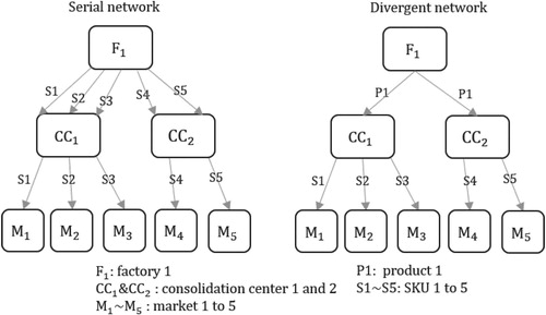
The demand is fulfilled through a three-stage distribution network consisting of factories, consolidation centres, and warehouses located in the local markets. Direct shipment and dual sourcing are not permitted. We assume batch production in the factories. The inventory is replenished from factories to consolidation centres and from consolidation centres to the warehouses periodically. On what basis the supply chain is configured determines the resulting network topologies: a serial network if the entire supply chain is configured for individual SKU, and divergent networks otherwise (see Figure 1 for the illustration).

Figure 1. Example of the divergent and the serial networks.

The locations and the amount of safety stock are determined using GSA. Following its concept, each of the potential stocking location i guarantees to fulfil the order placed from its downstream node in exactly $S_i$ periods. The service times of each location are then the decision variables to optimise, which imply the optimal inventory level in each node. Simpson (1958) proves that the optimal solution has an all-or-nothing property in a serial system; i.e. for a given stage i, the optimum occurs either when $S_i=0$, or when $S_i=S_{i-1}+T_i$, where $T_i$ stands for the lead time of the node i, and $S_{i-1}$ is the service time guaranteed by the direct predecessor. Inderfurth (1991) shows that this property is also valid for a divergent system. We notify the readers that we do not pursue modelling the inventory as rigorous as in a pure inventory control problem, but consider the impact of inventory in strategic decisions by exploiting the solution property of GSA. Assuming end market demand is immediately delivered, for a three-stage supply chain network, the all-or-nothing property leads to the four different policies of safety stock placement in Figure 2.

Figure 2. Four candidate optimal safety stock policies.

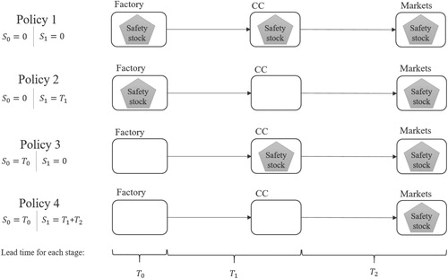
In addition, we consider two complementary modes: a responsive mode and an economic mode in production and transport, which differentiate the supply chain configurations. Table 1 shows the relation of these two modes in terms of cost and lead time parameters. The design of modes are based on the empirical information from Fichtinger, Chan, and Yates (2019) and they capture the relationship of prevalent supply chain strategies (Fisher 1997; Naylor, Naim, and Berry 1999). In supply chain segmentation, using production design/transport mode/inventory policy to differentiate the supply chains for different segments is commonly seen in the industry. For example, the case company in Fichtinger, Chan, and Yates (2019) segments the supply chains into lean/agile segments; each has a distinct production and transport mode. Philips restructures their distribution network, places safety stock point in different stages, adopting separate production strategies for different segments (Roy, Alicke, and Forsting 2017). The case company in Arampantzi, Minis, and Dikas (2019) considers also different production choices, transport modes and routes in their supply chain network transformation.

Table 1. Comparison of cost and lead time parameters of responsive and economic segment.

Process	Economic segment	Responsive segment
Production	Longer lead time	Shorter lead time
	Higher fixed cost	Lower fixed cost
	Lower variable cost	Higher variable cost
Distribution	Longer lead time	Shorter lead time
	Lower variable cost	Higher variable cost

Furthermore, we restrict each factory to be designed in either mode. The supply chain of a SKU or a product is configured either using an economic resource, i.e. economic mode of production and transport, or using a responsive resource. From the resource perspective, the network is primarily segmented into two groups: the group where economic mode is used, and the group where the responsive mode is used. Along with the inventory policy, there exist eight sub-groups. If location difference is also taken into consideration, there will be numerous groups which have distinct supply chain configurations. The studies which incorporate this idea include Langenberg, Seifert, and Tancrez (2012) who consider several supply chains from different combinations of production and transport resources, and Ernst and Cohen (1990) who aim to choose optimal inventory policies for a wide range of SKUs.

It follows that the number of options in terms of resource, inventory positioning, locations as well as any restriction on grouping affects the number of groups/segments that can be derived and the degree of differentiation of the overall supply chains. As a simple illustration, we consider the configuration decisions all made on SKU level versus all made on product level. The former would imply a serial network because the market/customer-specific decisions are made in the early stage and there is no chance to exploit the commonality of SKUs within a product from pooling, but in this case a higher level of differentiation is allowed. If all the decisions are made on product level, the commonality of SKUs within a product can be used in production and inventory, leading to a divergent network. In this case, all SKUs within a product share the same production/transport process and adopt the same inventory policy, thus the supply chain configurations are then more standardised. Following this thought, we develop four scenarios, which differ in terms of underlying assumptions in how the SKUs are grouped in the planning process. The four scenarios result in four different network types. We elaborate the details in Table 2.

Table 2. Four scenarios: assumptions of the planning approaches and resulting network types.

Scenario I	• Production location and mode are SKU specific. Each production batch is assigned to a particular market. Pooling in production is not possible
	• Replenishment is SKU specific. Inventory of SKUs can be kept in any of the three stages depending on which policy is chosen by the model. Inventory pooling is not possible
	• Transport is SKU specific.
	• The resulting network is a serial network, referred as Network I.
Scenario II	• Production location and mode are product specific. Each production batch is for aggregated demand of SKUs of a product.
	• Replenishment is product specific. Inventory of products have to be kept in upstream stages. Keeping inventory only in the market is not a choice. This means that the fourth inventory policy is not in consideration and SKUs of a product are forced to be pooled in upstream.
	• Transport is product specific.
	• The resulting network is a divergent network, referred as Network II.
Scenario III	• Production location and mode are product specific. Each production batch is for aggregated demand of SKUs of a product.
	• Replenishment is product specific. Inventory of products can be kept in any of the three stages. If an inventory policy is chosen for a product, all SKUs of the product follow the same policy.
	• Transport is product specific.
	• The resulting network is a divergent network, referred as Network III.
Scenario IV	• Production location and mode are product specific. Each production batch is for aggregated demand of SKUs of a product.
	• Replenishment is group (pool) specific. The optimisation model decides the inventory placement of SKUs in consideration of pooling benefits in upstream stages. The SKUs of a product which are placed in the same location are seen as a group. A possible solution for a product sold to five markets can be divided into two groups with three SKUs in one group and two SKUs in the other. The optimisation model can also decide to put all SKUs in a product in the same stock pool, ending up with only one group. SKUs in a group follow the same inventory policies.
	• Transport is group specific.
	• The resulting network is a divergent network, referred as Network IV.

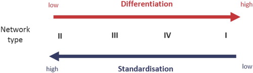
In each of the planning approaches, supply chains are optimally configured by minimising the total operating cost of serving these SKUs, which consists of the manufacturing, transport, and associated inventory costs. Each scenario implies a level of differentiation and standardisation in the resulting supply chain configurations. In Scenario I, the resource segment, inventory policy as well as allocation to facilities are decided on SKU basis. Examples of such an arrangement occurs in cases where each end market has specific requirements, e.g. ingredients, or packaging and labelling, and postponement of differentiation is not used. In this case, SKUs of a product can have different configurations. In Scenario II, the SKUs of a product are aggregated for planning. They share the same facilities and delivery route as well as a stock pool. The supply chains are configured differently among different products but are standardised for all SKUs of a product. Products that are managed under central production and distribution strategy end up in Scenario II. In Scenario III, the restriction of sharing a stock pool is released, but they still use the same inventory policy. This means that they either share a stock pool or all are kept only in the markets. Much of three-stage location-inventory literature that does not consider multi-echelon inventory placement naturally assumes that the middle stage is the stocking point. However, it is possible that the middle stage is not the optimal stage to place the safety stock. In this scenario, the assumption of upstream stages as stocking points is removed and the safety stock placement is decided by the optimisation model. In Scenario IV, the production facility and mode are selected on the product basis. The optimisation model then decides the transport route and where to place the safety stock of a SKU in consideration of the pooling benefits in the upstream stages. Scenario IV resembles the industrial cases where products are produced centrally but distributed worldwide via distribution centres or hubs (e.g. beverages). Figure 3 depicts the relative level of differentiation and standardisation of the resulting four networks.

Figure 3. Differentiation and standardisation levels of the four networks.

3.2. Notations

We use the notation below to model the four networks.

Indices/Sets	=
i	=	index of factories, i ∈$\mathcal{N}$
j	=	index of consolidation centres (CCs), j ∈$\mathcal{R}$
w	=	index of warehouses in the markets, w ∈$\mathcal{M}$
s	=	index of modes available; where $s=1\dots$ economic, $s=2\dots$ responsive
p	=	index of products, p ∈$\mathcal{P}$
e	=	index of inventory policies, e ∈$\mathcal{E}$
Parameters	=
${\lambda }_{wp}$	=	service factor for product p in market w, i.e. service factor of a specific SKU
${\mu }_{wp}$	=	mean of demand of product p in market w, i.e. mean of demand of a specific SKU
${\sigma }_{wp}$	=	standard deviation of demand of product p in market w, i.e. standard deviation of a specific SKU
$f_{is}$	=	fixed cost per lot at factory i in production mode s
$c_{is}^{\mathrm{f}\mathrm{a}\mathrm{c}}$	=	variable cost per unit at factory i in production mode s
$K_{is}$	=	capacity of factory i in production mode s
$Q_{iswp}$	=	production lot size of product p in market w in factory i operated in mode s
$Q_{isp}$	=	production lot size of product p in factory i operated in mode s
$c_{ijs}^{\mathrm{u}\mathrm{p}}$	=	transport cost per unit from factory i to CC j in transport mode s
$c_{jsw}^{\mathrm{d}\mathrm{n}}$	=	transport cost per unit from CC j to market w in transport mode s
h	=	stock holding cost rate in %
$r_j$	=	throughput cost per unit at CC j
$t_{is}^{\mathrm{f}\mathrm{a}\mathrm{c}}$	=	production lead time at factory i in production mode s
$t_{ijs}^{\mathrm{u}\mathrm{p}}$	=	transport lead time from factory i to CC j in transport mode s
$t_{jws}^{\mathrm{d}\mathrm{n}}$	=	transport time from CC j to market w in transport mode s
$S_{isp}^{\mathrm{f}\mathrm{a}\mathrm{c}}$	=	guaranteed service time at factory i in production mode s for product p
$S_{jsp}^{\mathrm{c}\mathrm{c}}$	=	guaranteed service time at CC j in transport mode s for product p
$S_{iswp}^{\mathrm{f}\mathrm{a}\mathrm{c}}$	=	guaranteed service time at factory i in production mode s for product p sold in market w
$S_{jswp}^{\mathrm{c}\mathrm{c}}$	=	guaranteed service time at CC j in transport mode s for product p sold in market w
${\mathrm{S}\mathrm{S}\mathrm{C}}_{isp}^{\mathrm{f}\mathrm{a}\mathrm{c}}$	=	safety stock cost at factory i in production mode s, for product p
${\mathrm{S}\mathrm{S}\mathrm{C}}_{jp}^{\mathrm{c}\mathrm{c}}$	=	safety stock cost at CC j for product p
${\mathrm{S}\mathrm{S}\mathrm{C}}_{wp}^{\mathrm{w}\mathrm{h}}$	=	safety stock cost at market w for product p
Decision variables	=
$X_{ijswp}$	=	1 if product p at market w is from factory i via CC j in segment s, and 0 otherwise
$X{s}_{ijsewp}$	=	1 if product p at market w is from factory i via CC j in segment s, using inventory policy e, and 0 otherwise
$X{d}_{ijsep}$	=	1 if product p is from factory i via CC j in segment s, using inventory policy e, and 0 otherwise
$Z_{is}$	=	1 if production mode s is chosen for factory i, and 0 otherwise
$Y_{isp}$	=	1 if factory i and segment s are chosen for product p, and 0 otherwise

3.3. Modeling network I

In this network, all the planning activities are performed on the SKU basis. The supply chain of a SKU is independent from another SKU. All the cost terms can therefore be calculated on the SKU basis. The concept of modelling the serial network has been presented in Fichtinger, Chan, and Yates (2019), but they consider only safety stock in the inventory associated cost. For completeness of our work, we restate the formulation of this network with introduction of our notations.

At first, the binary variable $X_{ijswp}$ is used in this case to represent the decision concerning the allocation of factories, consolidation centres, and mode to use for a SKU.

The production cost for each of SKU is the mean demand ${\mu }_{wp}$ times variable production cost per unit $c_{is}^{\mathrm{f}\mathrm{a}\mathrm{c}}$, plus average number of batches per period ${\mu }_{wp}/Q_{iswp}$ times the setup cost per batch $f_{is}$ on a given mode. We apply EOQ to compute batch quantity $Q_{iswp}$ prior to the optimisation model, which gives us $Q_{iswp}=\sqrt{2f_{is}{\mu }_{wp}/h{c}_{is}^{\mathrm{f}\mathrm{a}\mathrm{c}}}$. The production cost for product p sold in market w (SKU wp) produced in factory i operated in mode s is then ${\mu }_{wp}/Q_{iswp}+{\mu }_{wp}{c}_{is}^{\mathrm{f}\mathrm{a}\mathrm{c}}$.

The next cost terms in the model are the cost of using consolidation centre and transport cost, which consists of upstream and downstream delivery cost. These costs for SKU wp produced in factory i delivered to markets via consolidation centre j operated on mode s can be written as ${\mu }_{wp}{r}_j+{\mu }_{wp}{c}_{ijs}^{\mathrm{u}\mathrm{p}}+{\mu }_{wp}{c}_{jws}^{\mathrm{d}\mathrm{n}}$.

The associated inventory costs include cycle stock cost, pipeline stock cost, and safety stock cost. To compute those inventory costs, we evaluate the cost value of the products in each stage based on the stages they have been through and apply a holding cost rate h to the cost value. The cost value per unit of a product after the first stage, i.e. after being processed in the factory is ${\overline{c}}_{iswp}=f_{is}/Q_{iswp}+c_{is}^{\mathrm{f}\mathrm{a}\mathrm{c}}$. The cycle stock cost for a SKU wp produced in factory i operated in mode s is computed with average production cost per unit times the holding cost rate multiplied by half of the batch size: $\left(Q_{iswp}/2\right)\left({\overline{c}}_{iswp}h\right)$. Analogously, for SKU wp stocking in the stages of consolidation centres and warehouses in the local markets, the cost value per unit would be ${\overline{c}}_{ijswp}={\overline{c}}_{iswp}+c_{ijs}^{\mathrm{u}\mathrm{p}}+r_j$, and ${\overline{c}}_{ijswp}+c_{jws}^{\mathrm{d}\mathrm{n}}$, respectively.

The total pipeline stock cost for SKU wp produced in factory i delivered via consolidation centre j operated on mode s are $\left({\mu }_{wp}{t}_{ijs}^{\mathrm{u}\mathrm{p}}\right)\left({\overline{c}}_{iswp}h\right)+\left({\mu }_{wp}{t}_{jws}^{\mathrm{d}\mathrm{n}}\right)\left({\overline{c}}_{ijswp}h\right)$. The service times of SKU wp, $S_{iswp}^{\mathrm{f}\mathrm{a}\mathrm{c}}$ and $S_{jswp}^{\mathrm{c}\mathrm{c}}$ determine safety stock placement. The safety stock holding costs at the stage of factory, consolidation centre, and warehouse in the market area: (1) $\begin{array}{rl}& {\mathrm{S}\mathrm{S}\mathrm{C}}_{iswp}^{\mathrm{f}\mathrm{a}\mathrm{c}}\left(S_{iswp}^{\mathrm{f}\mathrm{a}\mathrm{c}}\right)=h\cdot {\overline{c}}_{iswp}{\lambda }_{wp}{\sigma }_{wp}\sqrt{t_{is}^{\mathrm{f}\mathrm{a}\mathrm{c}}-S_{iswp}^{\mathrm{f}\mathrm{a}\mathrm{c}}}.\end{array}$(1) (2) $\begin{array}{rl}& {\mathrm{S}\mathrm{S}\mathrm{C}}_{ijswp}^{\mathrm{c}\mathrm{c}}\left(S_{iswp}^{\mathrm{f}\mathrm{a}\mathrm{c}},S_{jswp}^{\mathrm{c}\mathrm{c}}\right)=h\cdot \left({\overline{c}}_{iswp}+c_{ijs}^{\mathrm{u}\mathrm{p}}+r_j\right){\lambda }_{wp}{\sigma }_{wp}\sqrt{S_{iswp}^{\mathrm{f}\mathrm{a}\mathrm{c}}+t_{ijs}^{\mathrm{u}\mathrm{p}}-S_{jswp}^{\mathrm{c}\mathrm{c}}}.\end{array}$(2) (3) $\begin{array}{rl}& {\mathrm{S}\mathrm{S}\mathrm{C}}_{ijswp}^{\mathrm{w}\mathrm{h}}\left(S_{jswp}^{\mathrm{c}\mathrm{c}}\right)=h\cdot \left({\overline{c}}_{iswp}+c_{ijs}^{\mathrm{u}\mathrm{p}}+c_{jswp}^{\mathrm{d}\mathrm{n}}+r_j\right){\lambda }_{wp}{\sigma }_{wp}\sqrt{S_{jswp}^{\mathrm{c}\mathrm{c}}+t_{jswp}^{\mathrm{d}\mathrm{n}}}.\end{array}$(3) Given the above formulation, the optimal total safety stock cost for SKU wp of a given configuration $(i,j,s)$, ${\mathrm{S}\mathrm{S}\mathrm{C}}_{ijswp}^{\ast }$, can be pre-calculated by evaluating all the corner values of $S_{iswp}^{\mathrm{f}\mathrm{a}\mathrm{c}}$ and $S_{jswp}^{\mathrm{c}\mathrm{c}}$. Putting all the cost components together, the model for Network I can be formulated as the following mixed-integer linear program: (4) $\begin{array}{rl}& \underset{X_{ijswp}}{min}\sum _{p\in P}\sum _{w\in M}\sum _{s\in S}\sum _{i\in N}\sum _{j\in R}{X}_{ijswp}({\mathrm{S}\mathrm{S}\mathrm{C}}_{ijswp}^{\ast }+\frac{{\mu }_{wp}}{Q_{wp}}{f}_{is}+{\mu }_p{c}_{is}^{\mathrm{f}\mathrm{a}\mathrm{c}}+{\mu }_{wp}{c}_{ijs}^{\mathrm{u}\mathrm{p}}+{\mu }_p{c}_{jsp}^{\mathrm{d}\mathrm{n}}+{\mu }_p{r}_j\\ & +\frac{Q_{iswp}}{2}({\overline{c}}_{iswp}h)+{\mu }_{wp}{t}_{ijs}^{\mathrm{u}\mathrm{p}}{\overline{c}}_{iswp}h+{\mu }_{wp}{t}_{jws}^{\mathrm{d}\mathrm{n}}{\overline{c}}_{ijswp}h)\end{array}$(4) Subject to: (5) $\begin{array}{rl}& \sum _{i\in N}\sum _{j\in R}\sum _{s\in S}{X}_{ijswp}=1\mathrm{\forall }w,p,\end{array}$(5) (6) $\begin{array}{rl}& X_{ijswp}\le Z_{is}\mathrm{\forall }i,j,s,w,p,\end{array}$(6) (7) $\begin{array}{rl}& \sum _{s\in S}{Z}_{is}=1\mathrm{\forall }i.\end{array}$(7) (8) $\begin{array}{rl}& \sum _{j\in R}\sum _{w\in P}\sum _{p\in P}{X}_{ijswp}{\mu }_{wp}\le K_{is}\mathrm{\forall }i,s,\end{array}$(8) (9) $\begin{array}{rl}& X_{ijswp},Z_{is}\in \{0,1\}\mathrm{\forall }i,j,s,w,p.\end{array}$(9) Constraint (5(5) $\begin{array}{rl}& \sum _{i\in N}\sum _{j\in R}\sum _{s\in S}{X}_{ijswp}=1\mathrm{\forall }w,p,\end{array}$(5) ) establishes the allocation of every SKU wp, to exactly one supply chain configuration, i.e. one factory, one consolidation centre, and one resource segment. Constraint (6(6) $\begin{array}{rl}& X_{ijswp}\le Z_{is}\mathrm{\forall }i,j,s,w,p,\end{array}$(6) ) ensures that a SKU can be allocated to a factory, if and only if the factory is operated in the same mode as the resource segment allocated to the SKU. Constraint (7(7) $\begin{array}{rl}& \sum _{s\in S}{Z}_{is}=1\mathrm{\forall }i.\end{array}$(7) ) ensures that each factory operates in only one segment s, and constraint (8(8) $\begin{array}{rl}& \sum _{j\in R}\sum _{w\in P}\sum _{p\in P}{X}_{ijswp}{\mu }_{wp}\le K_{is}\mathrm{\forall }i,s,\end{array}$(8) ) imposes the capacity limit on each factory operated in a certain mode.

3.4. Modeling network II and III

The main difference between Network II & III and Network I is the base on which the planning activities are performed. In these two networks, all of the planning are performed on the aggregated demand of a product. Product p is therefore the basis of calculation of each cost term. In this case, we use the binary variable $X{d}_{ijsep}$ to represent the decisions of the allocation of factories, consolidation centres, mode to use, and inventory placement applied for a product.

Applying the same logic as Network I, the costs of production, transport, and pipeline stock for a configuration $(i,j,s)$ are ${\mu }_p/Q_{isp}+{\mu }_p{c}_{is}^{\mathrm{f}\mathrm{a}\mathrm{c}}$, ${\mu }_p{r}_j+{\mu }_p{c}_{ijs}^{\mathrm{u}\mathrm{p}}+\sum _{w\in M}{\mu }_{wp}{c}_{jws}^{\mathrm{d}\mathrm{n}}$, and $\left({\mu }_p{t}_{ijs}^{\mathrm{u}\mathrm{p}}\right)\left({\overline{c}}_{isp}h\right)+\left(\sum _{w\in M}{\mu }_{wp}{t}_{jws}^{\mathrm{d}\mathrm{n}}\right)\left({\overline{c}}_{ijsp}h\right)$.

The decision of safety stock placement is influenced by both market and product demand, and pooling effect exists at upstream stages. We employ the subindex e in decision variable $X{d}_{ijsep}$ to represent each possible inventory policy. The safety stock costs, as determined by the service times $S_{isp}^{\mathrm{f}\mathrm{a}\mathrm{c}}$ and $S_{jsp}^{\mathrm{c}\mathrm{c}}$, are formulated as following mixed-integer linear program: (10) $\begin{array}{rl}{\mathrm{S}\mathrm{S}\mathrm{C}}_{isp}^{\mathrm{f}\mathrm{a}\mathrm{c}}& =h\cdot \sum _{j\in R}(X{d}_{ijs1p}+X{d}_{ijs2p})\cdot {\overline{c}}_{isp}\cdot \sqrt{\sum _{w\in M}{\sigma }_{wp}^2\cdot {\lambda }_{wp}^2}\sqrt{t_{isp}^{\mathrm{f}\mathrm{a}\mathrm{c}}}\end{array}$(10) (11) $\begin{array}{rl}{\mathrm{S}\mathrm{S}\mathrm{C}}_{jp}^{\mathrm{c}\mathrm{c}}& =h\cdot \left(X{d}_{ijs1p}\sqrt{\sum _{s\in S}\sum _{i\in N}\sum _{w\in M}{\overline{c}}_{ijsp}^2\cdot {\sigma }_{wp}^2\cdot {\lambda }_{wp}^2\cdot t_{ijs}^{\mathrm{u}\mathrm{p}}}\right.\\ & \left.+X{d}_{ijs3p}\sqrt{\sum _{s\in S}\sum _{i\in N}\sum _{w\in M}{\overline{c}}_{ijsp}^2\cdot {\sigma }_{wp}^2\cdot {\lambda }_{wp}^2\cdot (t_{isp}^{\mathrm{f}\mathrm{a}\mathrm{c}}+t_{ijs}^{\mathrm{u}\mathrm{p}})}\right)\end{array}$(11) (12) $\begin{array}{rl}{\mathrm{S}\mathrm{S}\mathrm{C}}_{wp}^{\mathrm{w}\mathrm{h}}& =h\cdot \sum _{s\in S}\sum _{i\in N}\sum _{j\in R}({\overline{c}}_{ijsp}+c_{jws}^{\mathrm{d}\mathrm{n}})\cdot {\sigma }_{wp}\cdot {\lambda }_{wp}\cdot (X{d}_{ijs1p}\sqrt{t_{jws}^{\mathrm{d}\mathrm{n}}}\\ & +X{d}_{ijs2p}\sqrt{t_{ijs}^{\mathrm{u}\mathrm{p}}+t_{jws}^{\mathrm{d}\mathrm{n}}}+X{d}_{ijs3p}\sqrt{t_{jws}^{\mathrm{d}\mathrm{n}}}+X{d}_{ijs4p}\sqrt{t_{isp}^{\mathrm{f}\mathrm{a}\mathrm{c}}+t_{ijs}^{\mathrm{u}\mathrm{p}}+t_{jws}^{\mathrm{d}\mathrm{n}}})\end{array}$(12) Equation (10(10) $\begin{array}{rl}{\mathrm{S}\mathrm{S}\mathrm{C}}_{isp}^{\mathrm{f}\mathrm{a}\mathrm{c}}& =h\cdot \sum _{j\in R}(X{d}_{ijs1p}+X{d}_{ijs2p})\cdot {\overline{c}}_{isp}\cdot \sqrt{\sum _{w\in M}{\sigma }_{wp}^2\cdot {\lambda }_{wp}^2}\sqrt{t_{isp}^{\mathrm{f}\mathrm{a}\mathrm{c}}}\end{array}$(10) ) sums up the safety stock cost in the factories, which incurs when inventory policy 1 or 2 is chosen. Whereas inventory policy 1 or 3 results in holding inventory in the consolidation centres; the cost is shown in Equation (11(11) $\begin{array}{rl}{\mathrm{S}\mathrm{S}\mathrm{C}}_{jp}^{\mathrm{c}\mathrm{c}}& =h\cdot \left(X{d}_{ijs1p}\sqrt{\sum _{s\in S}\sum _{i\in N}\sum _{w\in M}{\overline{c}}_{ijsp}^2\cdot {\sigma }_{wp}^2\cdot {\lambda }_{wp}^2\cdot t_{ijs}^{\mathrm{u}\mathrm{p}}}\right.\\ & \left.+X{d}_{ijs3p}\sqrt{\sum _{s\in S}\sum _{i\in N}\sum _{w\in M}{\overline{c}}_{ijsp}^2\cdot {\sigma }_{wp}^2\cdot {\lambda }_{wp}^2\cdot (t_{isp}^{\mathrm{f}\mathrm{a}\mathrm{c}}+t_{ijs}^{\mathrm{u}\mathrm{p}})}\right)\end{array}$(11) ). Equation (12(12) $\begin{array}{rl}{\mathrm{S}\mathrm{S}\mathrm{C}}_{wp}^{\mathrm{w}\mathrm{h}}& =h\cdot \sum _{s\in S}\sum _{i\in N}\sum _{j\in R}({\overline{c}}_{ijsp}+c_{jws}^{\mathrm{d}\mathrm{n}})\cdot {\sigma }_{wp}\cdot {\lambda }_{wp}\cdot (X{d}_{ijs1p}\sqrt{t_{jws}^{\mathrm{d}\mathrm{n}}}\\ & +X{d}_{ijs2p}\sqrt{t_{ijs}^{\mathrm{u}\mathrm{p}}+t_{jws}^{\mathrm{d}\mathrm{n}}}+X{d}_{ijs3p}\sqrt{t_{jws}^{\mathrm{d}\mathrm{n}}}+X{d}_{ijs4p}\sqrt{t_{isp}^{\mathrm{f}\mathrm{a}\mathrm{c}}+t_{ijs}^{\mathrm{u}\mathrm{p}}+t_{jws}^{\mathrm{d}\mathrm{n}}})\end{array}$(12) ) presents the safety stock cost in the markets, resulting from the four inventory policies. The model for Network II is then: $\begin{array}{rlr}& min\sum _{i\in N}\sum _{j\in R}\sum _{s\in S}\sum _{e\in E}\sum _{p\in P}X{d}_{ijsep}(\frac{{\mu }_p}{Q_{isp}}{f}_{is}+{\mu }_p{c}_{is}^{\mathrm{f}\mathrm{a}\mathrm{c}}+{\mu }_p{c}_{ijs}^{\mathrm{u}\mathrm{p}}+{\mu }_p{c}_{jws}^{\mathrm{d}\mathrm{n}}+{\mu }_p{r}_j& +\frac{Q_{isp}}{2}{\overline{c}}_{isp}h+{\mu }_p{t}_{ijs}^{\mathrm{u}\mathrm{p}}{\overline{c}}_{isp}h+{\mu }_p{t}_{jws}^{\mathrm{d}\mathrm{n}}{\overline{c}}_{ijsp}h)\\ & +\sum _{i\in N}\sum _{s\in S}\sum _{p\in P}{\mathrm{S}\mathrm{S}\mathrm{C}}_{isp}^{\mathrm{f}\mathrm{a}\mathrm{c}}+\sum _{j\in R}\sum _{p\in P}{\mathrm{S}\mathrm{S}\mathrm{C}}_{jp}^{\mathrm{c}\mathrm{c}}+\sum _{w\in M}\sum _{p\in P}{\mathrm{S}\mathrm{S}\mathrm{C}}_{wp}^{\mathrm{w}\mathrm{h}},\end{array}$ Subject to: (13) $\begin{array}{rl}& \sum _{i\in N}\sum _{j\in R}\sum _{s\in S}\sum _{e\in E}X{d}_{ijsep}=1\mathrm{\forall }p,\end{array}$(13) (14) $\begin{array}{rl}& X{d}_{ijsep}\le Z_{is}\mathrm{\forall }i,j,s,e,p,\end{array}$(14) (15) $\begin{array}{rl}& \sum _{s\in S}{Z}_{is}=1\mathrm{\forall }i,\end{array}$(15) (16) $\begin{array}{rl}& \sum _{j\in R}\sum _{e\in E}\sum _{p\in P}X{d}_{ijsep}{\mu }_p\le K_{is}\mathrm{\forall }i,s,\end{array}$(16) (17) $\begin{array}{rl}& X{d}_{ijs4p}=0\mathrm{\forall }i,j,s,p,\end{array}$(17) (18) $\begin{array}{rl}& X{d}_{ijsep},Z_{is}\in \{0,1\}\mathrm{\forall }i,j,s,p,e.\end{array}$(18) Constraints (13(13) $\begin{array}{rl}& \sum _{i\in N}\sum _{j\in R}\sum _{s\in S}\sum _{e\in E}X{d}_{ijsep}=1\mathrm{\forall }p,\end{array}$(13) ) – (16(16) $\begin{array}{rl}& \sum _{j\in R}\sum _{e\in E}\sum _{p\in P}X{d}_{ijsep}{\mu }_p\le K_{is}\mathrm{\forall }i,s,\end{array}$(16) ) resemble constraints (5(5) $\begin{array}{rl}& \sum _{i\in N}\sum _{j\in R}\sum _{s\in S}{X}_{ijswp}=1\mathrm{\forall }w,p,\end{array}$(5) ) – (8(8) $\begin{array}{rl}& \sum _{j\in R}\sum _{w\in P}\sum _{p\in P}{X}_{ijswp}{\mu }_{wp}\le K_{is}\mathrm{\forall }i,s,\end{array}$(8) ). Constraint (17(17) $\begin{array}{rl}& X{d}_{ijs4p}=0\mathrm{\forall }i,j,s,p,\end{array}$(17) ) forbids the use of the inventory policy where the safety stock is only placed in the local markets. This constraint is specific for the type II network to restrict the market demands fulfilled from a pooled stock. For Network III, we employ the same objective function and constraints (13(13) $\begin{array}{rl}& \sum _{i\in N}\sum _{j\in R}\sum _{s\in S}\sum _{e\in E}X{d}_{ijsep}=1\mathrm{\forall }p,\end{array}$(13) ) – (16(16) $\begin{array}{rl}& \sum _{j\in R}\sum _{e\in E}\sum _{p\in P}X{d}_{ijsep}{\mu }_p\le K_{is}\mathrm{\forall }i,s,\end{array}$(16) ) remain the same. Constraint (17(17) $\begin{array}{rl}& X{d}_{ijs4p}=0\mathrm{\forall }i,j,s,p,\end{array}$(17) ) is removed since inventory policy 4 can also be chosen under this network type.

3.5. Modeling network IV

In this network, decisions are made in two levels. $Y_{isp}$ represents the decision of allocating products to a factory and a segment. $X{s}_{ijsewp}$ is associated with the adoption of the inventory policy and the allocation of the consolidation centre for a certain SKU. The calculation of production cost, transport cost and warehousing cost remains the same as Network II and III. The safety stock placements (10(10) $\begin{array}{rl}{\mathrm{S}\mathrm{S}\mathrm{C}}_{isp}^{\mathrm{f}\mathrm{a}\mathrm{c}}& =h\cdot \sum _{j\in R}(X{d}_{ijs1p}+X{d}_{ijs2p})\cdot {\overline{c}}_{isp}\cdot \sqrt{\sum _{w\in M}{\sigma }_{wp}^2\cdot {\lambda }_{wp}^2}\sqrt{t_{isp}^{\mathrm{f}\mathrm{a}\mathrm{c}}}\end{array}$(10) ) – (12(12) $\begin{array}{rl}{\mathrm{S}\mathrm{S}\mathrm{C}}_{wp}^{\mathrm{w}\mathrm{h}}& =h\cdot \sum _{s\in S}\sum _{i\in N}\sum _{j\in R}({\overline{c}}_{ijsp}+c_{jws}^{\mathrm{d}\mathrm{n}})\cdot {\sigma }_{wp}\cdot {\lambda }_{wp}\cdot (X{d}_{ijs1p}\sqrt{t_{jws}^{\mathrm{d}\mathrm{n}}}\\ & +X{d}_{ijs2p}\sqrt{t_{ijs}^{\mathrm{u}\mathrm{p}}+t_{jws}^{\mathrm{d}\mathrm{n}}}+X{d}_{ijs3p}\sqrt{t_{jws}^{\mathrm{d}\mathrm{n}}}+X{d}_{ijs4p}\sqrt{t_{isp}^{\mathrm{f}\mathrm{a}\mathrm{c}}+t_{ijs}^{\mathrm{u}\mathrm{p}}+t_{jws}^{\mathrm{d}\mathrm{n}}})\end{array}$(12) ) are reformulated using the alternative decision variable $X{s}_{ijsewp}$. Given the fact that $X{s}_{ijs1wp}+X{s}_{ijs2wp}=X{s}_{ijs1wp}^2+X{s}_{ijs2wp}^2$, we obtain: (19) $\begin{array}{rl}{\mathrm{S}\mathrm{S}\mathrm{C}}_{isp}^{\mathrm{f}\mathrm{a}\mathrm{c}}& =h\cdot {\overline{c}}_{isp}\cdot \sqrt{\sum _{j\in R}\sum _{w\in M}(X{s}_{ijs1wp}^2+X{s}_{ijs2wp}^2)\cdot {\sigma }_{wp}^2\cdot {\lambda }_{wp}^2}\sqrt{t_{isp}^{\mathrm{f}\mathrm{a}\mathrm{c}}}\end{array}$(19) (20) $\begin{array}{rl}{\mathrm{S}\mathrm{S}\mathrm{C}}_{jp}^{\mathrm{c}\mathrm{c}}& =h\cdot \left(\sqrt{\sum _{s\in S}\sum _{i\in N}\sum _{w\in M}X{s}_{ijs1wp}^2\cdot {\overline{c}}_{ijswp}^2\cdot {\sigma }_{wp}^2\cdot {\lambda }_{wp}^2\cdot t_{ijs}^{\mathrm{u}\mathrm{p}}}\right.\\ & \left.+\sqrt{\sum _{s\in S}\sum _{i\in N}\sum _{w\in M}X{s}_{ijs3wp}^2\cdot {\overline{c}}_{ijswp}^2\cdot {\sigma }_{wp}^2\cdot {\lambda }_{wp}^2\cdot (t_{isp}^{\mathrm{f}\mathrm{a}\mathrm{c}}+t_{ijs}^{\mathrm{u}\mathrm{p}})}\right)\end{array}$(20) (21) $\begin{array}{rl}{\mathrm{S}\mathrm{S}\mathrm{C}}_{wp}^{\mathrm{w}\mathrm{h}}& =h\sum _{s\in S}\sum _{i\in N}\sum _{j\in R}({\overline{c}}_{ijswp}+c_{jws}^{\mathrm{d}\mathrm{n}})\cdot {\sigma }_{wp}\cdot {\lambda }_{wp}\cdot (X{s}_{ijs1wp}\sqrt{t_{jws}^{\mathrm{d}\mathrm{n}}}\\ & +X{s}_{ijs2wp}\sqrt{t_{ijs}^{\mathrm{u}\mathrm{p}}+t_{jws}^{\mathrm{d}\mathrm{n}}}+X{s}_{ijs3wp}\sqrt{t_{jws}^{\mathrm{d}\mathrm{n}}}+X{s}_{ijs4wp}\sqrt{t_{isp}^{\mathrm{f}\mathrm{a}\mathrm{c}}+t_{ijs}^{\mathrm{u}\mathrm{p}}+t_{jws}^{\mathrm{d}\mathrm{n}}})\end{array}$(21) The configuration decision $X{s}_{ijsewp}$ for Network IV appears inside the square root terms, which results in non-linearity in the objective function. We use the approach proposed by Atamtürk, Berenguer, and Shen (2012), introducing three auxiliary variables $O_{isp}$, $U_{jp}$ and $V_{jp}$ to replace the square root terms in Equations (19(19) $\begin{array}{rl}{\mathrm{S}\mathrm{S}\mathrm{C}}_{isp}^{\mathrm{f}\mathrm{a}\mathrm{c}}& =h\cdot {\overline{c}}_{isp}\cdot \sqrt{\sum _{j\in R}\sum _{w\in M}(X{s}_{ijs1wp}^2+X{s}_{ijs2wp}^2)\cdot {\sigma }_{wp}^2\cdot {\lambda }_{wp}^2}\sqrt{t_{isp}^{\mathrm{f}\mathrm{a}\mathrm{c}}}\end{array}$(19) ) and (20(20) $\begin{array}{rl}{\mathrm{S}\mathrm{S}\mathrm{C}}_{jp}^{\mathrm{c}\mathrm{c}}& =h\cdot \left(\sqrt{\sum _{s\in S}\sum _{i\in N}\sum _{w\in M}X{s}_{ijs1wp}^2\cdot {\overline{c}}_{ijswp}^2\cdot {\sigma }_{wp}^2\cdot {\lambda }_{wp}^2\cdot t_{ijs}^{\mathrm{u}\mathrm{p}}}\right.\\ & \left.+\sqrt{\sum _{s\in S}\sum _{i\in N}\sum _{w\in M}X{s}_{ijs3wp}^2\cdot {\overline{c}}_{ijswp}^2\cdot {\sigma }_{wp}^2\cdot {\lambda }_{wp}^2\cdot (t_{isp}^{\mathrm{f}\mathrm{a}\mathrm{c}}+t_{ijs}^{\mathrm{u}\mathrm{p}})}\right)\end{array}$(20) ), turning the optimisation model into conic quadratic mixed-integer program (CQMIP). Equations (19(19) $\begin{array}{rl}{\mathrm{S}\mathrm{S}\mathrm{C}}_{isp}^{\mathrm{f}\mathrm{a}\mathrm{c}}& =h\cdot {\overline{c}}_{isp}\cdot \sqrt{\sum _{j\in R}\sum _{w\in M}(X{s}_{ijs1wp}^2+X{s}_{ijs2wp}^2)\cdot {\sigma }_{wp}^2\cdot {\lambda }_{wp}^2}\sqrt{t_{isp}^{\mathrm{f}\mathrm{a}\mathrm{c}}}\end{array}$(19) ) and (20(20) $\begin{array}{rl}{\mathrm{S}\mathrm{S}\mathrm{C}}_{jp}^{\mathrm{c}\mathrm{c}}& =h\cdot \left(\sqrt{\sum _{s\in S}\sum _{i\in N}\sum _{w\in M}X{s}_{ijs1wp}^2\cdot {\overline{c}}_{ijswp}^2\cdot {\sigma }_{wp}^2\cdot {\lambda }_{wp}^2\cdot t_{ijs}^{\mathrm{u}\mathrm{p}}}\right.\\ & \left.+\sqrt{\sum _{s\in S}\sum _{i\in N}\sum _{w\in M}X{s}_{ijs3wp}^2\cdot {\overline{c}}_{ijswp}^2\cdot {\sigma }_{wp}^2\cdot {\lambda }_{wp}^2\cdot (t_{isp}^{\mathrm{f}\mathrm{a}\mathrm{c}}+t_{ijs}^{\mathrm{u}\mathrm{p}})}\right)\end{array}$(20) ) become ${\mathrm{S}\mathrm{S}\mathrm{C}}_{isp}^{\mathrm{f}\mathrm{a}\mathrm{c}}=h{\overline{c}}_{isp}\sqrt{t_{isp}^{\mathrm{f}\mathrm{a}\mathrm{c}}}\cdot O_{isp}$ and ${\mathrm{S}\mathrm{S}\mathrm{C}}_{jp}^{\mathrm{c}\mathrm{c}}=h\cdot (U_{jp}+V_{jp})$. Along with the transformation, the optimisation model for Network IV is: $\begin{array}{rl}& min\sum _{i\in N}\sum _{j\in R}\sum _{s\in S}\sum _{e\in E}\sum _{p\in P}\sum _{w\in M}X{s}_{ijsewp}\\ & \times (\frac{{\mu }_p}{Q_{isp}}{f}_{is}+{\mu }_p{c}_{is}^{\mathrm{f}\mathrm{a}\mathrm{c}}+{\mu }_{wp}{c}_{ijs}^{\mathrm{u}\mathrm{p}}+{\mu }_{wp}{c}_{jws}^{\mathrm{d}\mathrm{n}}+{\mu }_{wp}{r}_j+\frac{Q_{isp}}{2}{\overline{c}}_{isp}h+{\mu }_{wp}{t}_{ijs}^{\mathrm{u}\mathrm{p}}{\overline{c}}_{isp}h+{\mu }_p{t}_{jws}^{\mathrm{d}\mathrm{n}}{\overline{c}}_{ijswp}h)\\ & +\sum _{i\in N}\sum _{s\in S}\sum _{p\in P}h{\overline{c}}_{isp}\sqrt{t_{isp}^{\mathrm{f}\mathrm{a}\mathrm{c}}}\cdot O_{isp}+\sum _{j\in R}\sum _{p\in P}h\cdot (U_{jp}+V_{jp})+\sum _{w\in M}\sum _{p\in P}{\mathrm{S}\mathrm{S}\mathrm{C}}_{wp}^{\mathrm{w}\mathrm{h}},\end{array}$ Subject to: (22) $\begin{array}{rl}& \sum _{i\in N}\sum _{j\in R}\sum _{s\in S}\sum _{e\in E}X{s}_{ijsewp}=1\mathrm{\forall }w,p,\end{array}$(22) (23) $\begin{array}{rl}& Y_{isp}\le Z_{is}\mathrm{\forall }i,s,p,\end{array}$(23) (24) $\begin{array}{rl}& \sum _{s\in S}{Z}_{is}=1\mathrm{\forall }i,\end{array}$(24) (25) $\begin{array}{rl}& \sum _{j\in R}\sum _{e\in E}\sum _{p\in P}\sum _{w\in M}X{s}_{ijsewp}{\mu }_{wp}\le K_{is}\mathrm{\forall }i,s\end{array}$(25) (26) $\begin{array}{rl}& X{s}_{ijsewp}\le Y_{isp}\mathrm{\forall }i,j,s,e,w,p\end{array}$(26) (27) $\begin{array}{rl}& \sum _{i\in N}\sum _{s\in S}{Y}_{isp}=1\mathrm{\forall }p,\end{array}$(27) (28) $\begin{array}{rl}& \sum _{j\in R}\sum _{w\in M}(X{s}_{ijs1wp}^2+X{s}_{ijs2wp}^2)\cdot {\sigma }_{wp}^2\cdot {\lambda }_{wp}^2\le O_{isp}^2\mathrm{\forall }i,s,p\end{array}$(28) (29) $\begin{array}{rl}& \sum _{s\in S}\sum _{i\in N}\sum _{w\in M}X{s}_{ijs1wp}^2\cdot {\overline{c}}_{ijswp}^2\cdot {\sigma }_{wp}^2\cdot {\lambda }_{wp}^2\cdot t_{ijs}^{\mathrm{u}\mathrm{p}}\le U_{jp}^2\mathrm{\forall }j,p\end{array}$(29) (30) $\begin{array}{rl}& \sum _{s\in S}\sum _{i\in N}\sum _{w\in M}X{s}_{ijs3wp}^2\cdot {\overline{c}}_{ijswp}^2\cdot {\sigma }_{wp}^2\cdot {\lambda }_{wp}^2\cdot (t_{isp}^{\mathrm{f}\mathrm{a}\mathrm{c}}+t_{ijs}^{\mathrm{u}\mathrm{p}})\le V_{jp}^2\mathrm{\forall }j,p\end{array}$(30) (31) $\begin{array}{rl}& X{s}_{ijsewp},Y_{isp},Z_{is}\in \{0,1\}\mathrm{\forall }i,j,s,p\end{array}$(31) (32) $\begin{array}{rl}& O_{isp},U_{jp},V_{jp}\ge 0\mathrm{\forall }i,j,s,p\end{array}$(32) The constraints (22(22) $\begin{array}{rl}& \sum _{i\in N}\sum _{j\in R}\sum _{s\in S}\sum _{e\in E}X{s}_{ijsewp}=1\mathrm{\forall }w,p,\end{array}$(22) ) – (25(25) $\begin{array}{rl}& \sum _{j\in R}\sum _{e\in E}\sum _{p\in P}\sum _{w\in M}X{s}_{ijsewp}{\mu }_{wp}\le K_{is}\mathrm{\forall }i,s\end{array}$(25) ) are analogous to the constraints (13(13) $\begin{array}{rl}& \sum _{i\in N}\sum _{j\in R}\sum _{s\in S}\sum _{e\in E}X{d}_{ijsep}=1\mathrm{\forall }p,\end{array}$(13) ) – (16(16) $\begin{array}{rl}& \sum _{j\in R}\sum _{e\in E}\sum _{p\in P}X{d}_{ijsep}{\mu }_p\le K_{is}\mathrm{\forall }i,s,\end{array}$(16) ) in type II and III networks. The constraints which are specific for Network IV are constraints (26(26) $\begin{array}{rl}& X{s}_{ijsewp}\le Y_{isp}\mathrm{\forall }i,j,s,e,w,p\end{array}$(26) ) and (27(27) $\begin{array}{rl}& \sum _{i\in N}\sum _{s\in S}{Y}_{isp}=1\mathrm{\forall }p,\end{array}$(27) ) which force a product to be produced in one factory and operated through one mode regardless the markets it is delivered to, and the quadratic constraints (28(28) $\begin{array}{rl}& \sum _{j\in R}\sum _{w\in M}(X{s}_{ijs1wp}^2+X{s}_{ijs2wp}^2)\cdot {\sigma }_{wp}^2\cdot {\lambda }_{wp}^2\le O_{isp}^2\mathrm{\forall }i,s,p\end{array}$(28) ) – (30(30) $\begin{array}{rl}& \sum _{s\in S}\sum _{i\in N}\sum _{w\in M}X{s}_{ijs3wp}^2\cdot {\overline{c}}_{ijswp}^2\cdot {\sigma }_{wp}^2\cdot {\lambda }_{wp}^2\cdot (t_{isp}^{\mathrm{f}\mathrm{a}\mathrm{c}}+t_{ijs}^{\mathrm{u}\mathrm{p}})\le V_{jp}^2\mathrm{\forall }j,p\end{array}$(30) ) which define auxiliary variables.

According to Atamtürk, Berenguer, and Shen (2012), the main advantage of CQMIP formulation is that it is flexible from the modelling perspective and can be solved directly using standard optimisation software package such as CPLEX and Mosek. The computational efficiency of CQMIP can be strengthened with polymatroid inequalities, which are added as cutting planes to facilitate the computational process. For the technique details, we refer readers to Edmonds (1970) and Atamtürk, Berenguer, and Shen (2012).

4. Numerical study

The numerical study presented in this paper is based on two types of data: demand profile, and configuration-related cost and lead time parameters. We employ the dataset from the case company used in Fichtinger, Chan, and Yates (2019) but adapt it to serve the purpose of our analyses. The adaption includes decreasing the network scale and extend it for a distribution network. Specifically, we arbitrarily select three factories out of six, 21 markets out of 43, 224 SKU out of the original 6013. We then arbitrarily assign them to the 21 different markets, yielding 50 different products which are sold to a different number of markets. The assignment is conducted based on the premise that regardless which planning approaches are adopted, the performance can be improved by segmentation and network optimisation. This is the logical consideration for firms when developing their network and exploring the segmentation benefits. On the other hand, we use only a subset of the original network as the original scale is far too complex for extension to a distribution network and adds negligible value to our study. Such an approach is often seen in the network-related studies (e.g. Çelebi 2015; Peres et al. 2017; Ghavamifar, Makui, and Taleizadeh 2018 for recent applications).

The resulting dataset is referred as adapted real data. We then create another dataset by setting up equal cost and lead time parameters for arcs and nodes of the same type. We create these parameters using the weighted-average (weighted by factory capacities) values from the adapted real data. In the real world, the value of such operational parameters in each node and arc in the network usually varies due to different market regions and the geographic distribution of the sites (Fichtinger, Chan, and Yates 2019). Factors such as technologies and regulations in different regions can contribute to the variance. We construct this dataset to isolate the effect of this variance from the impact of demand characteristics. We refer to this dataset as synthetic data, consisting of an adapted real demand profile, and synthetic network-related operational parameters. Our analysis is mainly based on the adapted real data and the synthetic data is used only in some of the analysis for comparison purpose. For the remaining parameters that are not included in these datasets, h and ${\lambda }_{wp}$, we apply commonly used values, 0.25 and 3. Table 3 summarises the values of the different parameters for the arcs and nodes in the datasets, where a dash ‘–’ means that we use the adapted real value for that item.

Table 3. Values in the datasets.

Notation	Adapted real values value range	Synthetic values
Set
$\mathcal{N}$	3 locations	–
$\mathcal{R}$	3 locations	–
$\mathcal{M}$	21 locations	–
$\mathcal{S}$	2 modes	–
$\mathcal{P}$	50 products	–
$\mathcal{I}$	4 policies	–
Demand parameters
${\mu }_p$	[11, $28\mathrm{k}$]k units	–
${\sigma }_p$	[1, $21\mathrm{k}$]k units	–
cv	[0.01, 3]	–
Cost
$f_{i1}$	[60, 750]€/lot	500€/lot
$f_{i2}$	[12, 149]€/lot	100€/lot
$K_{i1}$	132, 000 k units	–
$K_{i2}$	170, 000 k units	–
$c_{i1}^{\mathrm{f}\mathrm{a}\mathrm{c}}$	[4.8, 11.8]€/$10\mathrm{k}$ units	9€/$10\mathrm{k}$ units
$c_{i2}^{\mathrm{f}\mathrm{a}\mathrm{c}}$	[7.1, 18.7]€/$10\mathrm{k}$ units	13.4€/$10\mathrm{k}$ units
$c_{ij1}^{\mathrm{u}\mathrm{p}}$	[0.09, 0.46]€/$10\mathrm{k}$ units	0.25€/$10\mathrm{k}$ units
$c_{ij2}^{\mathrm{u}\mathrm{p}}$	[0.19, 1.65]€/$10\mathrm{k}$ units	0.57€/$10\mathrm{k}$ units
$c_{j1wp}^{\mathrm{d}\mathrm{n}}$	[0.04, 3.95]€/$10\mathrm{k}$ units	0.70€/$10\mathrm{k}$
$c_{j2wp}^{\mathrm{d}\mathrm{n}}$	[0.07, 12.24]€/$10\mathrm{k}$ units	2.2€/$10\mathrm{k}$
$r^j$	0.1€/$10\mathrm{k}$ units	–
Lead time
$t_{i1}^{\mathrm{f}\mathrm{a}\mathrm{c}}$	1 month	–
$t_{i2}^{\mathrm{f}\mathrm{a}\mathrm{c}}$	0.2 month	–
$t_{ij1}^{\mathrm{u}\mathrm{p}}$	[0.10, 1.50] months	0.6 month
$t_{ij2}^{\mathrm{u}\mathrm{p}}$	[0.02, 0.50] months	0.15 month
$t_{j1p}^{\mathrm{d}\mathrm{n}}$	[0.04, 0.36] months	0.21 month
$t_{j2p}^{\mathrm{d}\mathrm{n}}$	[0.04, 0.18] months	0.08 month
Other parameters
h	–	0.25
${\lambda }_p$	–	3

To examine the robustness of our statements and conclusion, we also test the main part of our analysis on a few different datasets. These include two randomly generated data based on the methods in Park, Lee, and Sung (2010) and Shahabi et al. (2014). We demonstrate the results of these two datasets in the appendix to show the general consistency of our findings and observations.

We write the setting of our models in python code and solve the optimisation models in Gurobi on a 2.60 GHz laptop with 8 GB RAM. With the data used in numerical study, Network I, II, III can be solved within 5 minutes. In comparison, the global optimum for CQMIP is harder to obtain within a reasonable amount of time. Therefore, we use the solution with 0.1% gap or solution with time limited to 30,000 seconds. In general, we are able to get the solution with 0.1% gap within 10,000 seconds.

Table 4 presents the results of optimal supply chain configurations under the four different planning scenarios using the adapted real data. We can see that Scenario I has a greater number of SKUs allocated to the responsive segment compared with the other three. This is because in the absence of pooling, using the economic mode which increases safety stock required could be expensive for SKUs with higher demand variability. We also observe that there are nearly no SKUs assigned to inventory policy 1 and 2, indicating stocking in the factories is unfavourable. This result is in line with the findings of Hua and Willems (2016) which point out that in a serial system unless cost at the upstream stage is relatively low or its lead time is relatively long, it is not worthwhile to decouple the total supply chain lead time and hold safety stock at the upstream stage. This explains why inventory policy 4 is assigned for all SKUs in Scenario I where inventory pooling is absent. We numerically verify this finding for divergent systems. As the allocations of inventory policies in the other three scenarios show, the benefits of pooling can make stocking in the upstream stages a more attractive option. Nevertheless, the comparison of SKU allocation to inventory segments in Scenario II and III shows that pooling inventory in the upstream stages is the only favourable solution for some SKUs not all SKUs. Forcing all SKUs of a product to share the same stock pool can lead to increase in safety stock cost. In Scenario III, nearly half of SKUs in the product portfolio choose to keep inventory in the markets, while in Scenario IV where the SKUs are segmented for inventory decisions, benefits from inventory pooling can be better exploited and thus more SKUs are assigned to place inventory in the upstream stages. The difference between Scenario III and IV captures the extent to which segmenting SKUs of a product for different inventory policies is beneficial.

Table 4. The operating cost and the number of SKUs allocated to inventory and resource segments.

		Resource segment		Inventory segment
Scenario	Operating cost	Economic	Responsive	1	2	3	4
I	471, 941	17	207	0	0	2	222
II	481, 733	56	168	0	6	218	0
III	466, 520	56	168	0	0	111	113
IV	463, 139	54	170	0	9	126	89

4.1. Comparison of total cost

The cost difference between Scenario I and II explains whether loss of differentiation or loss of pooling benefits in all levels are dominant. The cost difference between Scenario I and IV shows if loss of aggregated production and transport benefits outweighs loss of differentiation on these two levels. If the latter effect is strong, Scenario I costs less than Scenario IV. Otherwise we expect Scenario IV has the least cost since, in terms of how SKUs can be grouped in inventory placement, it is less restrictive and either Scenario I or II might have the most. As shown in Table 5, the lower cost in production and cycle stock of Scenario II does not offset the higher cost in transport and safety stock compared with Scenario I. In this case, loss of differentiation dominates loss of pooling benefits, and safety stock placement drives the cost difference among Scenario II, III, and IV. The influence of other cost elements resulting from different allocations of sites are dependent on the cost structure. In this dataset, the effect of other factors is trivial.

Table 5. The cost breakdown.

Scenario	Production	Transport	Throughput	Cycle stock	Pipeline stock	Safety stock
I	245, 912	34, 301	3, 268	15, 370	24, 439	148, 651
II	243, 020	37, 374	3, 268	11, 905	25, 006	161, 160
III	243, 020	37, 374	3, 268	11, 905	25, 006	145, 946
IV	243, 029	34, 489	3, 268	11, 900	25, 150	145, 302

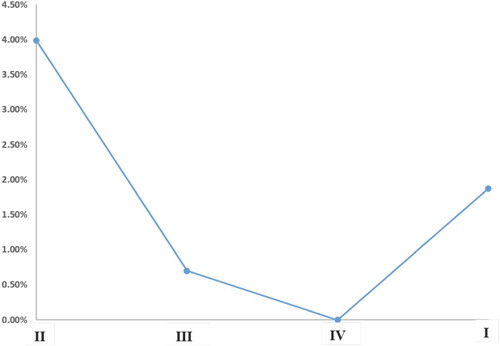
Figure 4 shows that by comparing the operating costs of these four scenarios, the trade-off between standardisation and differentiation can be visualised as a U-shape curve. We infer that the lowest point in this U-shape curve, which is not included in this study, is where the SKUs are optimally grouped for production batch and inventory pooling. At this point, the full potential of segmentation can be realised. This point is between the cost of Scenario I and the cost of Scenario IV. We notify the readers that we approximate the lowest point with Scenario IV because optimal grouping of SKUs for all configuration decisions requires joint optimisation of production batch and inventory pooling, which greatly increases complexity of the model and does not guarantee to be solvable. The grouping of Scenario I, II, and III are then suboptimal. With the current parameters, Scenario I is less suboptimal than Scenario II and the curve leans towards the right side because higher differentiation is preferred. We expect the shape of this curve changes with different parameters applied. For example, we find that with certain parameters the total cost of Scenario I is less than Scenario III, implying that the loss of differentiation outweighs loss of aggregation and pooling benefits and the lowest point in the U-shape is closer to Scenario I than Scenario IV. In the following, we examine the impact of cost synergy, different network parameters, and resource options on the shape of this curve.

Figure 4. % increase in cost compared with Scenario IV.

We first look at the perspective of cost synergy. In our study, two parameters, holding cost rate and fixed cost of production have direct influence on the strength of cost synergy. The benefit from optimally pooling the products increases with higher holding cost rates, and the fixed production cost influences the benefits of pooled production.

Figure 5(a) shows when holding cost rate $0.01\mathrm{\%}$, the curve is rather flat because cost increase by suboptimal grouping decisions are marginal. As the holding cost rate increases, the curve bends (or tilt) more. This shows that inventory decisions become more relevant with the increase of the holding cost rates, and hence the cost differences among the suboptimal grouping decisions in Network I, II and III are more apparent.

Figure 5. % increase in cost for Network I, II and III compared with cost for Network IV. (a) % increase in cost with respect to the % change of holding cost rate. (b) % increase in cost with respect to the % change of fixed cost in both modes. (c) % increase in cost compared with Scenario IV based on the both datasets and (d) % increase in cost compared with Scenario IV with segmented resources and single resource.

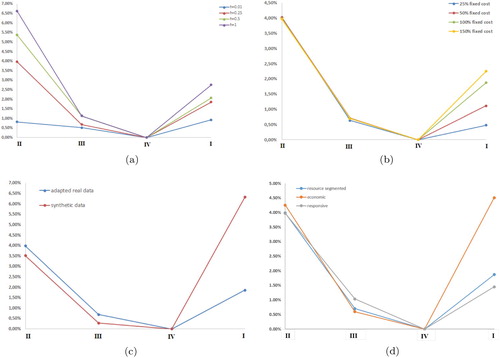
The change of curvature as the fixed cost increases is less apparent (see Figure 5(b)) on the left-hand side since Scenario II, III and IV have the same production setting. On the other hand, the impact of an increase in fixed cost on total production cost is different under Scenario I and IV since they use different production settings with respect to how the production batches are formed.

The network parameters give information on operational characteristics of each node and arc, and have implications on the degree of centralisation a network should have. For products sold to adjoining markets, managing SKUs through the same facilities to enjoy benefits from pooling in production could render good cost performance. If the demand points are far away from each other, it may be better to produce them separately and holding the stock in the nearby facilities. In the case of a supply chain design configured on the basis of product level, it is not possible to separate them in different processes. We demonstrate the impact purely from the demand aspect and from both demand and supply chains in Figure 5(c) by comparing the cost differences of these four scenarios using both datasets. The results from the synthetic data capture the impact of varying demand characteristics on the cost performance. Under this dataset, the benefits of pooling outweigh the benefits of differentiation; therefore Scenario I without any pooling possibility can be relatively costly. In addition, as the difference of SKUs in this dataset only exhibits in demand characteristics, the benefit of segmenting SKUs of a product according to different inventory policies is reduced compared to the benefits under the adapted real dataset. However, pooling all SKUs in the upstream stages (scenario II) still incurs a noticeable cost increase. This shows that even after eliminating the difference in operational characteristics, pooling the inventory in the upstream stages does not necessarily give benefits for some SKUs where demand characteristics are too different. We will elaborate this point further in Section 4.3.

The resource also affects the balance of differentiation and standardisation. Figure 5(d) compares the % cost increase of a segmented network under different scenarios with that of networks designed in a single mode, either economic or responsive. It shows the more responsive the production and transport, the less advantageous it is to group and manage SKUs through the same process, and thus the % cost increase of Scenario I is the least when only the responsive mode is used. This is because economies of scale reduce in a more responsive mode, and supply chains are less prone to longer lead times. When only the economic mode is used, the cost increase from both total pool solution (Scenario II) or total non-pool solutions (Scenario I) are similarly suboptimal. In this case, segmenting SKUs of a product for different configurations becomes more important.

4.2. Impact of resource segmentation

In this section, we analyse the value of resource segmentation under the four scenarios. The analysis is performed on both datasets but here we focus on the results from the adapted real dataset. We assume an unsegmented network is the network where either a economic mode or a responsive mode is used. Table 6 summarises the comparison of the cost performance and allocation of inventory policies of a segmented network and a unsegmented network for all four scenarios. The cost improvement of segmenting networks through the use of resources ranges from $1.74\mathrm{\%}$ to $6.6\mathrm{\%}$. We note to the readers that the significance of segmentation benefits naturally depends on the parameters in the problem setting.

Table 6. Operating cost of a single resource segment in use compared with optimally segmented SC and allocations of resource (economic on the left and responsive on the right) and inventory segments for optimally segmented SC.

				Inventory segment
Network	Resource (allocation)	Operating cost	% Cost increase	1	2	3	4
I	segmented ($17|207$)	471, 941	–	0	0	2	222
	economic	503, 363	$6.66\mathrm{\%}$	0	0	0	224
	responsive	480, 153	$1.74\mathrm{\%}$	0	0	3	221
II	segmented ($56|168$)	481, 734	–	0	6	218	0
	economic	502, 132	$4.23\mathrm{\%}$	0	0	224	0
	responsive	492, 092	$2.15\mathrm{\%}$	0	4	220	0
III	segmented ($56|168$)	466, 519	–	0	0	111	113
	economic	484, 508	$3.86\mathrm{\%}$	0	0	115	109
	responsive	478, 174	$2.50\mathrm{\%}$	0	0	101	123
IV	segmented ($54|170$)	463, 139	–	0	0	126	89
	economic	481, 642	$4.00\mathrm{\%}$	0	0	148	76
	responsive	473, 283	$2.19\mathrm{\%}$	0	0	123	92

The difference among Network II, III, and IV in terms of allocation of resources and inventory segments is minor because they have same production setting which dominates selection of resource segments. In contrast, we see a substantial difference when comparing the results of these three divergent networks with that of Network I. The number of SKUs allocated to the economic segment is more than triple the number in network I. This shows that the opportunity of pooling in production and inventory allows firms to gain more cost benefits if they operate purely in the economic mode whereas the need to cope with demand variability and the resulting benefits of segmentation under the responsive mode is reduced. Pooling demand in the process, on the other hand, implies that the demand characteristics faced in the supply chain becomes more homogenous. We therefore expect the divergent networks to be more sensitive (in terms of cost performance) to the selection of resources if a single type is used. We observe this trend only in the results when the synthetic dataset is used. The results from real adapted data where the complication of geographic difference is involved do not exhibit an apparent preference towards either segment.

4.3. Impact of demand characteristics

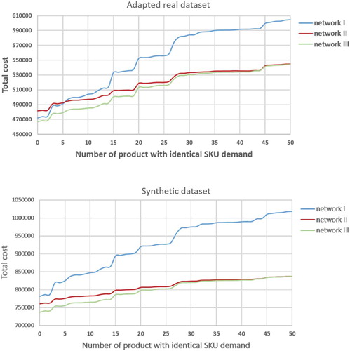
In this section, we investigate the impact of divergence within a product portfolio on the cost performance under different planning approaches. Specifically, we use a series of synthesized demand profiles, each exhibiting a certain level of divergence. We compare the cost performance of Scenario I, II, and III on those portfolios. To synthesize the demand profiles, we use our demand profile from the databases as a benchmark profile in which demands of the SKUs of a product are dissimilar. We then average the mean SKUs demand and variance of first, second, and third products sequentially to create the first, second, and third synthesized demand profile. In total, 50 demand profiles are synthesized. The benchmark profile has the most heterogeneous product portfolio and the $50\mathrm{t}\mathrm{h}$ demand profile is the most homogenous one because all the SKU demands of the products are identical. The aggregated volume and variability in these 51 demand profiles are the same.

Figure 6 shows the change of cost for these 51 product portfolios under Scenario I, II, and III. With both datasets, we observe that the total costs of Network II and III gradually converge when there are more products with identical SKU demands in the product portfolio. This indicates that the benefits of pooling inventory is higher when the pooled demands are more homogenous. At the same time, we also see there is a greater marginal cost increase in Network I than in the other two networks. This is because when the SKUs in a product have relatively similar demand characteristics, cost synergy from operating them through a standardised process outweighs the benefits of differentiating them through individually tailored processes. When the demand characteristics of SKUs in a product are divergent enough, the benefits of managing them through Network I start to be more apparent.

Figure 6. Total cost of product portfolios differing in number of products with identical SKU demands.

4.4. Being responsive: expediting processes with responsive resource vs. inventory pooling

The benefit of segmentation lies in grouping similar items together and aligning them with the correct operations strategy. A way of dealing with the increasing cost from high-demand variability is assigning each of them individually to a responsive process. In this way, the decline in cost associated with the buffer (i.e. safety stock) required for variability is in exchange of higher variable cost in production and transport. Another way is to handle these items as a pool which can reduce the impact of variability without the need to switch from an economic process to a responsive process. Pooling and optimal resource alignment are hence the major measures for firms to deal with demand variability. It is however not totally obvious how the benefit of one measure affects that of the other measure. We therefore examine the degree of pooling effects with respect to the demand variability where there is the possibility of optimal resource allocation. The previous analyses indicate that the heterogeneity of demand characteristics and the difference in operational attributes affect pooling benefits. To isolate these factors, we assume a hypothetical product sold to five markets with identical market demands and analyse the impact of optimally aligned supply chains on the benefits of inventory pooling using costs and lead times of the synthetic dataset. In this case, three divergent networks, II, III and IV, result in same total cost. We examine product demand with a mean ranging from 10 k to 10 m with different cv. Table 7 shows the results for the product with a mean demand $=1\mathrm{m}$ and cv ranging from 0.01 to 3.

Table 7. % Cost saving from inventory pooling for mean product demand 1 m when supply chain is operated with optimal mode.

	Optimal mode
product cv	Serial (non-pool)	Divergent (pool)	% cost diff.
0.01	Economic	Economic	$23.77\mathrm{\%}$	11.9
0.1	Economic	Economic	$25.15\mathrm{\%}$	12.6
0.2	Economic	Economic	$26.55\mathrm{\%}$	13.3
0.3	Economic	Economic	$27.80\mathrm{\%}$	14.0
0.4	Economic	Economic	$28.94\mathrm{\%}$	14.5
0.5	Economic	Economic	$29.98\mathrm{\%}$	15.0
0.6	Responsive	Economic	$29.75\mathrm{\%}$	14.9
0.7	Responsive	Economic	$28.73\mathrm{\%}$	14.3
0.8	Responsive	Economic	$27.80\mathrm{\%}$	13.9
0.9	Responsive	Economic	$26.93\mathrm{\%}$	13.6
1.0	Responsive	Economic	$26.13\mathrm{\%}$	13.0
1.1	Responsive	Economic	$25.38\mathrm{\%}$	12.6
1.2	Responsive	Economic	$24.69\mathrm{\%}$	12.3
1.3	Responsive	Economic	$24.04\mathrm{\%}$	12.0
1.4	Responsive	Economic	$23.43\mathrm{\%}$	11.7
1.5	Responsive	Economic	$22.86\mathrm{\%}$	11.4
1.6	Responsive	Economic	$22.32\mathrm{\%}$	11.1
1.7	Responsive	Economic	$21.82\mathrm{\%}$	10.9
1.8	Responsive	Economic	$21.34\mathrm{\%}$	10.6
1.9	Responsive	Economic	$20.89\mathrm{\%}$	10.4
2.0	Responsive	Economic	$20.46\mathrm{\%}$	10.2
2.1	Responsive	Economic	$20.06\mathrm{\%}$	10.0
2.2	Responsive	Economic	$19.67\mathrm{\%}$	9.8
2.3	Responsive	Responsive	$19.69\mathrm{\%}$	9.9
2.4	Responsive	Responsive	$19.95\mathrm{\%}$	10.0
2.5	Responsive	Responsive	$20.20\mathrm{\%}$	10.1
2.6	Responsive	Responsive	$20.44\mathrm{\%}$	10.21
2.7	Responsive	Responsive	$20.68\mathrm{\%}$	10.45
2.8	Responsive	Responsive	$20.90\mathrm{\%}$	10.55
2.9	Responsive	Responsive	$21.12\mathrm{\%}$	10.68
3.0	Responsive	Responsive	$21.33\mathrm{\%}$	10.8

It can be observed how the degree of demand uncertainty affects the optimal segment used. In the presence of an inventory pooling opportunity, the impact of demand uncertainty is reduced and supply chains are sustained with longer lead times of the economic segment. Extra cost for using the responsive process is only necessary when cv is higher than 2.3. The red bars along each row show the trend of pooling benefits with respect to demand variability. We further interpret this trend with the graphic expression in Figure 7.

Figure 7. Graphic expression of pooling benefit in relation to optimal modes and demand variability.

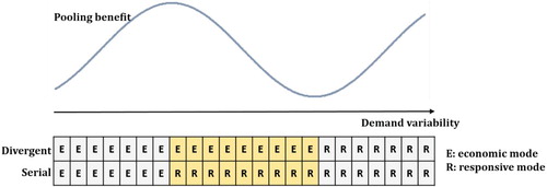
In the area where demand variability is relatively low, the economic mode is the optimal mode for both network typologies. As demand variability rises to a certain level, the increase of inventory costs in the serial system calls for the use of the responsive mode, while the economic mode remains as the optimal mode for the divergent network because the impact of variability has been reduced through pooling. In this region, although both the cost of required inventory incurred under economic mode for the divergent network and that under responsive mode for the serial network increase as demand variability increases, the rate of the increase under economic mode is greater than that under the responsive mode. Hence a decreasing trend can be observed when comparing the total cost of these two networks. When demand variability reaches to a even higher level, it becomes optimal to pool the demands and use the responsive mode for the divergent network to mitigate the impact of variability. Because in this area both networks have the same optimal mode, an increasing trend of pooling benefits is observed when variability keeps rising.

5. Conclusion

This study makes several contributions to the existing literature in SC&OM with respect to supply chain segmentation. Foremost, we identify the commonality of segmentation in different areas and make the bridge among these previously separate research streams. We demonstrate through different scenarios that supply chain segmentation faces the common trade-off as segmentation in other areas. More importantly, we show quantitatively how the factors such as demand heterogeneity, network characteristics, and pooling affect the balance of this trade-off.

As another contribution, we develop mathematical models which integrate segmentation and configuration decisions for divergent networks, which are more commonly adopted in the real world (Dominguez, Framinan, and Cannella 2014). Unlike the two-step approach applied in many SC segmentation studies, our models optimally align the process segments and SKU segments. Our process segments, differing from other quantitative literature in segmentation, cover a wider perspective in supply chain configuration. For the divergent network where inventory pooling decision is optimised, we formulate it as a conic quadratic mixed-integer program and strengthen the conic constraints with the polymatroid inequalities. This model also contributes to existing location-inventory literature by considering the possibility of inventory placement and pooling at different stages.

Several observations and managerial implications are derived through the numerical analyses with four different focuses: (1) the impact of operational difference, resource, cost parameters on the balance of the trade-off; (2) the impact of resource segmentation; (3) the impact of demand heterogeneity; (4) the impact of demand variability. The first part aims at understanding the trade-off of standardisation and differentiation in a system by comparing the different grouping assumptions and conducting sensitivity analysis. The results imply that there may exist a most effective configuration (the lower point of U-curve) where SKUs are optimally grouped for the different stages of supply chains. The analysis also shows how the magnitude of the other suboptimal configurations are influenced by the cost parameters. The second part analyses the benefits of segmenting the network into responsive and economic supply chains in consideration of demand pooling. The analysis reveals that the benefits of segmenting supply chains compared with using single resource are dependent not only on the pooling opportunity but also on operational characteristics of each site within a network. The third part looks into the impact of demand heterogeneity on grouping/pooling SKUs. We find that the more homogenous the product portfolio a firm has, the higher benefits can be obtained by grouping them in the same stock pool. Finally, we show that in the presence of responsive resource and pooling opportunity, there is interdependency of these two as the measures in coping with demand variability.

The managerial implications are especially relevant for firms which deliver one (type of) product to multiple markets since they have to decide on how and where to group these products in order to exploit the commonality. Such supply chain features are commonly seen in pharmaceutical and consumer-oriented industries. In addition, we provide managers an insight into the implications of planning approaches in the resulting physical networks. For managers who face the complex problems in classifying supply chain configurations, our study renders a quantitative benchmark to support rational decision-making by enabling the evaluation of numerous grouping scenarios and sensitivity analysis.

An immediate extension of this study is to integrate the pooling decisions for both inventory and production. This integration will guarantee the optimal grouping of SKUs for different configurations. The complication of such a model may require a heuristics approach to obtain the solutions. The other possibility for extension is to model production in more detail, e.g. using a queueing model. In our study, we evaluate the segmentation on the network level and model the production, transport, and inventory on the strategic level since the inclusion of some operational decisions would heavily burden the optimisation processes and would result in unsolvable models. Additionally, in this study we consider only two resource segments: a segment with economic mode, and a segment with responsive mode, in order to develop the detailed insights from our results. It would be meaningful to consider more modes when the complexity cost of adding more modes and the consolidation effect by using the same mode are factored in the model.

Disclosure statement

No potential conflict of interest was reported by the author(s).

Appendix

Computational results of the tested datasets

Additional datasets are used to test the robustness of our findings and exam the general consistency of our observations. We select the computational results of two datasets which are randomly generated based on the strategy used in Park, Lee, and Sung (2010) and Shahabi et al. (2014). Table 8 summarises the parameters used to generate the data. We define $V_0$ as the total volume of demands per period. The potential locations of the factories, consolidation centres, and warehouses in the markets are randomly generated according to a uniform distribution over the square of (0, 10]. In addition, the transport costs between each pair of factory and consolidation centre, $D_{ij}$, and consolidation centre and warehouse, $D_{jw}$ are assumed to be based on kilometre and proportional the Euclidean distances between the generated locations. Per unit distance per unit demand transportation costs, α, are set to be 1.0. A dash ‘–’ means that the parameter setting is the same as that in the left column.

Table A1. Data generation.

	Tested dataset A	Tested dataset B
network ($\mathcal{N},\mathcal{R},\mathcal{M},\mathcal{P}$)	$(5,5,10,15)$	$(6,3,8,10)$
mean demand per period	${\mu }_{wp}=U[50,5000]$	–
coefficient of variation of demand	$v_{wp}=U[0.1,2]$	–
service factor	${\lambda }_{wp}=U[1,3]$	–
factory capacity	$K_{is}=V_0/3$	–
setup cost per batch (economic) at factory i	$f_{i1}=U[500,1000]$	–
setup cost per batch (express) at factory i	$f_{i2}=f_{i1}U[0.1,0.2]$
production cost per unit (economic) at factory i	$c_{i1}=U[20,40]$
production cost per unit (express) at factory i	$c_{i2}=c_{i1}(1+U[0.2,0.5\left]\right)$	$c_{i2}=1.5c_{i1}(1+U[0.2,0.5\left]\right)$
production lead time (economic) at factory i	$t_{i1}=U[2,5]$	–
production lead time (express) at factory i	$t_{i2}=t_{i1}U[0.1,0.3]$	–
transport cost (economic) per unit from factory i to DC j	$c_{ij1}=0.5\alpha D_{ij}$	–
transport cost (express) per unit from factory i to DC j	$c_{ij2}=c_{ij1}(1+U[0.2,0.5\left]\right)$	$c_{ij2}=1.2c_{ij1}(1+U[0.2,0.5\left]\right)$
transport cost (economic) per unit from DC j to factory i	$c_{jw1}=\alpha D_{jw}$	$c_{jw1}=0.2\alpha D_{jw}$
transport cost (express) per unit from DC j to warehouse w	$c_{jw2}=c_{jw1}(1+U[0.2,0.5\left]\right)$	–
order lead time (economic) from factory i to DC j	$t_{ij1}=U[0.5,2]$	–
order lead time (express) from factory i to DC j	$t_{ij2}=t_{ij1}U[0.1,0.3]$	–
order lead time (economics) from DC j to warehouse w	$t_{jw1}=U[0.1,0.5]$	$t_{jw1}=U[1,5]$
order lead time (express) from DC j to warehouse w	$t_{jw2}=t_{jw1}U[0.1,0.3]$	–

Computation results of the tested datasets A and B corresponding to Section 4.1 are presented in the following tables.

Table A2. The operating cost and the number of SKUs allocated to inventory and resource segments for dataset A.

		Resource segment		Inventory segment
Scenario	Operating cost	Economic	Responsive	1	2	3	4
I	24, 546, 986	49	101	0	0	0	150
II	22, 241, 047	80	70	0	0	150	0
III	22, 241, 047	80	70	0	0	150	0
IV	22, 237, 883	80	70	0	0	147	3

Table A3. The cost breakdown for dataset A.

Scenario	Production	Transport	Throughput	Cycle stock	Pipeline stock	Safety stock
I	13, 305, 763	2, 030, 344	34, 700	223, 197	1, 341, 449	7, 611, 533
II	12, 287, 773	2, 420, 175	34, 700	86, 019	1, 868, 727	5, 543, 654
III	12, 287, 773	2, 420, 175	34, 700	86, 019	1, 868, 727	5, 543, 654
IV	12, 287, 773	2, 411, 978	34, 700	86, 019	1, 870, 302	5, 547, 112

Table A4. The operating cost and the number of SKUs allocated to inventory and resource segments for dataset B.

		Resource segment		Inventory segment
Scenario	operating cost	Economic	Responsive	1	2	3	4
I	17, 054, 204	49	31	0	0	0	80
II	17, 523, 098	56	24	0	0	80	0
III	17, 478, 972	56	24	0	0	64	16
IV	17, 219, 645	56	24	0	16	41	23

Table A5. The cost breakdown for dataset B.

Scenario	Production	Transport	Throughput	Cycle stock	Pipeline stock	Safety stock
I	5, 852, 918	799, 254	21, 602	143, 293	3, 358, 848	6, 878, 289
II	5, 734, 004	570, 647	21, 602	51, 594	4, 342, 603	6, 802, 648
III	5, 734, 004	570, 647	21, 602	51, 594	4, 342, 603	6, 758, 522
IV	5, 752, 925	712, 095	21, 602	53, 268	3, 801, 789	6, 877, 964

References

- Abedi, Arash, and Weihang Zhu. 2017. “An Optimisation Model for Purchase, Production and Distribution in Fish Supply Chain – A Case Study.” International Journal of Production Research 55 (12): 3451–3464.
- Arampantzi, Christina, Ioannis Minis, and Georgios Dikas. 2019. “A Strategic Model for Exact Supply Chain Network Design and its Application to a Global Manufacturer.” International Journal of Production Research 57 (5): 1371–1397.
- Atamtürk, Alper, Gemma Berenguer, and Zuo-Jun (Max) Shen. 2012. “A Conic Integer Programming Approach to Stochastic Joint Location-Inventory Problems.” Operations Research 60 (2): 366–381.
- Babai, M. Z., T. Ladhari, and I. Lajili. 2015. “On the Inventory Performance of Multi-Criteria Classification Methods: Empirical Investigation.” International Journal of Production Research 53 (1): 279–290.
- Berry, William L., Terry Hill, and Jay E. Klompmaker. 1999. “Aligning Marketing and Manufacturing Strategies with the Market.” International Journal of Production Research 37 (16): 3599–3618.
- Berry, William L., Jay E. Klompmaker, Cecil C. Bozarth, and Terence J. Hill. 1991. “Factory Focus: Segmenting Markets From an Operations Perspective.” Journal of Operations Management 10 (3): 363–387.
- Bhattacharya, Arijit, Bijan Sarkar, and Sanat K. Mukherjee. 2007. “Distance-Based Consensus Method for ABC Analysis.” International Journal of Production Research 45 (15): 3405–3420.
- Billington, Corey, Gianpaolo Callioni, Barrett Crane, John D. Ruark, Julie Unruh Rapp, Trace White, and Sean P. Willems. 2004. “Accelerating the Profitability of Hewlett-Packard's Supply Chains.” INFORMS Journal on Applied Analytics 34 (1): 59–72.
- Çelebi, Dilay. 2015. “Inventory Control in a Centralized Distribution Network Using Genetic Algorithms: A Case Study.” Computers & Industrial Engineering 87: 532–539.
- Childerhouse, Paul, James Aitken, and Denis R. Towill. 2002. “Analysis and Design of Focused Demand Chains.” Journal of Operations Management 20 (6): 675–689.
- Christopher, Martin, and Denis R. Towill. 2001. “An Integrated Model for the Design of Agile Supply Chains.” International Journal of Physical Distribution & Logistics Management 31 (4): 235–246.
- Christopher, Martin, Denis R. Towill, James Aitken, and Paul Childerhouse. 2009. “Value Stream Classification.” Journal of Manufacturing Technology Management 20 (4): 460–474.
- Dawe, Peter, Alicia Pittman, and Elfrun von Koeller. 2015. “Segmentation in the Consumer Supply Chain: One Size Does Not Fit All.” Technical Report . The Boston Consulting Group. Accessed 20 September 2018. https://www.bcg.com/publications/2015/segmentation-in-the-consumer-supply-chain-one-size-does-not-fit-all.aspx.
- Dominguez, Roberto, Jose M. Framinan, and Salvatore Cannella. 2014. “Serial Vs. Divergent Supply Chain Networks: A Comparative Analysis of the Bullwhip Effect.” International Journal of Production Research 52 (7): 2194–2210.
- Edmonds, J. 1970. “Submodular Functions, Matroids, and Certain Polyhedra.” In Combinatorial Structures and Their Applications, edited by R. K. Guy, H. Hanai, N. Sauer, and J. Schönheim, 69–87. New York: Gordon and Brach.
- Ernst, Ricardo, and Morris A. Cohen. 1990. “Operations Related Groups (ORGs): A Clustering Procedure for Production/Inventory Systems.” Journal of Operations Management 9 (4): 574–598.
- Farasyn, Ingrid, Salal Humair, Joel I. Kahn, John J. Neale, Oscar Rosen, John Ruark, William Tarlton, Wim Van de Velde, Glenn Wegryn, and Sean P. Willems. 2011. “Inventory Optimization at Procter & Gamble: Achieving Real Benefits through User Adoption of Inventory Tools.” INFORMS Journal on Applied Analytics 41 (1): 66–78.
- Fichtinger, Johannes, Claire Chan, and Nicky Yates. 2019. “A Joint Network Design and Multi-Echelon Inventory Optimisation Approach for Serial Supply Chain Segmentation.” International Journal of Production Economics 209: 103–111.
- Fisher, Marshall L. 1997. “What is the Right Supply Chain for Your Product?” Harvard Business Review 75 (2): 105–116.
- Flores, Benito E., and D. Clay Whybark. 1986. “Multiple Criteria ABC Analysis.” International Journal of Operations & Production Management 6 (3): 38–46.
- Ghavamifar, Ali, Ahmad Makui, and Ata Allah Taleizadeh. 2018. “Designing a Resilient Competitive Supply Chain Network under Disruption Risks: A Real-World Application.” Transportation Research Part E: Logistics and Transportation Review 115: 87–109.
- Godsell, Janet, Thomas Diefenbach, Chris Clemmow, Denis R. Towill, and Martin Christopher. 2011. “Enabling Supply Chain Segmentation through Demand Profiling.” International Journal of Physical Distribution & Logistics Management 41 (3): 296–314.
- Goldsby, Thomas J., Stanley E. Griffis, and Anthony S. Roath. 2006. “Modeling Lean, Agile, and Leagile Supply Chain Strategies.” Journal of Business Logistics 27 (1): 57–80.
- Graves, Stephen C., and Sean P. Willems. 2003. “Supply Chain Design: Safety Stock Placement and Supply Chain Configuration.” Handbooks in Operations Research and Management Science 11: 95–132.
- Guajardo, Jose A., and Morris A. Cohen. 2018. “Service Differentiation and Operating Segments: A Framework and An Application to After-Sales Services.” Manufacturing & Service Operations Management 20 (3): 440–454.
- Hallgren, Mattias, and Jan Olhager. 2006. “Differentiating Manufacturing Focus.” International Journal of Production Research 44 (18–19): 3863–3878.
- Herer, Yale T., Michal Tzur, and Enver Yücesan. 2002. “Transshipments: An Emerging Inventory Recourse to Achieve Supply Chain Leagility.” International Journal of Production Economics 80 (3): 201–212.
- Hua, N. Grace, and Sean P. Willems. 2016. “Analytical Insights Into Two-Stage Serial Line Supply Chain Safety Stock.” International Journal of Production Economics 181: 107–112.
- Inderfurth, Karl. 1991. “Safety Stock Optimization in Multi-Stage Inventory Systems.” International Journal of Production Economics 24 (1–2): 103–113.
- Jayaswal, Sachin, and Elizabeth M. Jewkes. 2016. “Price and Lead Time Differentiation, Capacity Strategy and Market Competition.” International Journal of Production Research 54 (9): 2791–2806.
- Kehoe, D. F., S. Dani, H. Sharifi, N. D. Burns, and C. J. Backhouse. 2007. “Demand Network Alignment: Aligning the Physical, Informational and Relationship Issues in Supply Chains.” International Journal of Production Research 45 (5): 1141–1160.
- Kellar, Gregory M., George G. Polak, and Xinhui Zhang. 2016. “Synchronization, Cross-docking, and Decoupling in Supply Chain Networks.” International Journal of Production Research 54 (9): 2585–2599.
- Langenberg, Kerstin U., Ralf W. Seifert, and Jean-Sébastien Tancrez. 2012. “Aligning Supply Chain Portfolios with Product Portfolios.” International Journal of Production Economics 135 (1): 500–513.
- Li, Yao, Yang Cheng, Qing Hu Shenghan Zhou, Lei Ma, and Ming K. Lim. 2019. “The Influence of Additive Manufacturing on the Configuration of Make-to-Order Spare Parts Supply Chain under Heterogeneous Demand.” International Journal of Production Research 57 (11): 3622–3641.
- Li, D., and C. O'Brien. 2001. “A Quantitative Analysis of Relationships Between Product Types and Supply Chain Strategies.” International Journal of Production Economics 73 (1): 29–39.
- Liao, Shu-Hsien, Chia-Lin Hsieh, and Peng-Jen Lai. 2011. “An Evolutionary Approach for Multi-Objective Optimization of the Integrated Location – Inventory Distribution Network Problem in Vendor-Managed Inventory.” Expert Systems with Applications 38 (6): 6768–6776.
- Lim, Michael K., Ho-Yin Mak, and Zuo-Jun Max Shen. 2017. “Agility and Proximity Considerations in Supply Chain Design.” Management Science 63 (4): 1026–1041.
- Lovell, Antony, Richard Saw, and Jennifer Stimson. 2005. “Product Value-Density: Managing Diversity through Supply Chain Segmentation.” The International Journal of Logistics Management 16 (1): 142–158.
- Macchion, Laura, Rosanna Fornasiero, and Andrea Vinelli. 2017. “Supply Chain Configurations: A Model to Evaluate Performance in Customised Productions.” International Journal of Production Research 55 (5): 1386–1399.
- Martinez-Olvera, C., and D. Shunk. 2006. “Comprehensive Framework for the Development of a Supply Chain Strategy.” International Journal of Production Research 44 (21): 4511–4528.
- Mason-Jones, Rachel, Ben Naylor, and Denis R. Towill. 2000. “Lean, Agile Or Leagile? Matching Your Supply Chain to the Marketplace.” International Journal of Production Research 38 (17): 4061–4070.
- Mohammaddust, Faeghe, Shabnam Rezapour, Reza Zanjirani Farahani, Mohammad Mofidfar, and Alex Hill. 2017. “Developing Lean and Responsive Supply Chains: A Robust Model for Alternative Risk Mitigation Strategies in Supply Chain Designs.” International Journal of Production Economics 183: 632–653.
- Naylor, J. Ben, Mohamed M. Naim, and Danny Berry. 1999. “Leagility: Integrating the Lean and Agile Manufacturing Paradigms in the Total Supply Chain.” International Journal of Production Economics 62 (1–2): 107–118.
- Olbert, Henning, Margarita Protopappa-Sieke, and Ulrich W. Thonemann. 2016. “Analyzing the Effect of Express Orders on Supply Chain Costs and Delivery Times.” Production and Operations Management 25 (12): 2035–2050.
- Olivares Aguila, Jessica, and Waguih ElMaraghy. 2018. “Structural Complexity and Robustness of Supply Chain Networks Based on Product Architecture.” International Journal of Production Research 56 (20): 6701–6718.
- Park, Sukun, Tae-Eog Lee, and Chang Sup Sung. 2010. “A Three-Level Supply Chain Network Design Model with Risk-Pooling and Lead Times.” Transportation Research Part E: Logistics and Transportation Review 46 (5): 563–581.
- Peres, Igor T., Hugo M. Repolho, Rafael Martinelli, and Nathália J. Monteiro. 2017. “Optimization in Inventory-Routing Problem with Planned Transshipment: A Case Study in the Retail Industry.” International Journal of Production Economics 193: 748–756.
- Protopappa-Sieke, Margarita, and Ulrich W. Thonemann, eds. 2017. Supply Chain Segmentation: Best-in-Class Cases, Practical Insights and Foundations. Springer.
- Puga, Matías Schuster, Stefan Minner, and Jean-Sébastien Tancrez. 2019. “Two-Stage Supply Chain Design with Safety Stock Placement Decisions.” International Journal of Production Economics 209: 183–193.
- Roy, Sanchay, Knut Alicke, and Maren Forsting. 2017. “Philips Segmentation Case Study.” In Supply Chain Segmentation, edited by M. Protopappa-Sieke and U. Thonemann, 27–36. Springer, Cham.
- Shahabi, Mehrdad, Avinash Unnikrishnan, Ehsan Jafari-Shirazi, and Stephen D. Boyles. 2014. “A Three Level Location-Inventory Problem with Correlated Demand.” Transportation Research Part B: Methodological 69: 1–18.
- Sheikhzadeh, Alireza, and Manuel D. Rossetti. 2015. “Segmentation Methods for Large-Scale Multi-Echelon Service Parts Logistics Systems.” In Proceedings of the 2015 Industrial and Systems Engineering Research Conference, Nashville, Tennessee, May 30 – June 2, edited by S. Cetinkaya and J.K. Ryan.
- Simpson, Kenneth F. 1958. “In-Process Inventories.” Operations Research 6 (6): 863–873.
- Skinner, Wickham. 1969. “Manufacturing – Missing Link in Corporate Strategy.” Harvard Business Review 47 (3): 136–145.
- Skinner, Wickham. 1974. “The Focused Factory.” Harvard Business Review 52 (3): 113–121.
- Truong, Tu H., and Farhad Azadivar. 2005. “Optimal Design Methodologies for Configuration of Supply Chains.” International Journal of Production Research 43 (11): 2217–2236.
- van Kampen, Tim J., Renzo Akkerman, and Dirk Pieter van Donk. 2012. “SKU Classification: A Literature Review and Conceptual Framework.” International Journal of Operations & Production Management 32 (7): 850–876.
- von Falkenhausen, Christian J. F. 2017. “Three Essays on Aligning Supply Chain Strategies with the Business Environment.” PhD diss., University of Mannheim.
- You, Fengqi, and Ignacio E. Grossmann. 2010. “Integrated Multi-Echelon Supply Chain Design with Inventories under Uncertainty: MINLP Models, Computational Strategies.” AIChE Journal 56 (2): 419–440.
- Zhang, Lianfeng, Xiao You, Jianxin Jiao, and Petri Helo. 2009. “Supply Chain Configuration with Co-Ordinated Product, Process and Logistics Decisions: An Approach Based on Petri Nets.” International Journal of Production Research 47 (23): 6681–6706.