Co-procurement: making the most of collaborative procurement

Abstract

While the procurement decision is generally made by individual buyers, this study investigates how a group of buyers can make a shared decision. We call this collaborative approach, co-procurement. A mathematical model is formulated for the decision of procurement from multiple suppliers. The model is solved for individual buyers. The outcome shows the optimal number of items a buyer should buy from different suppliers such that the total cost is minimised for that buyer. Next, it is investigated how a group of buyers could make this decision together. The proposed model takes into account transaction costs of collaboration, to determine the optimal size of the collaboration and the involved parties. The idea is new in the old direction of procurement and it introduces the concept of transaction costs in this area and analyses its impact on the optimal collaboration size and mix. A case study from Dutch Food Valley is provided to investigate the benefits of co-procurement and validate the developed structure. The results indicate that co-procurement can bring considerable cost-savings through consolidation of orders and more efficient transportation schedules. A sensitivity analysis is conducted to determine the impact of changes in the transaction cost in favour of the co-procurement.

KEYWORDS:

• Supply chain management
• procurement
• collaboration
• pricing
• transaction cost

1. Introduction and theoretical background

To maintain their competitive advantage in a global economy, companies have to compete through their supply chains (Martínez-Olvera and Davizon-Castillo 2015), which means they are constantly looking for opportunities to reduce costs in their supply chain. There are many aspects of supply chain management that can be approached in different ways to optimise and enhance the system’s capabilities. Classical approaches include targeting the familiar problems most buyers face, namely procurement lot-sizing, supplier selection and complex transportation networks, with multiple levels of intermediate facilities and modes.

However, there is a limit to the profits that can be realised by individual companies trying to optimise their supply chain. A collaborative approach involving multiple buyers may yield positive results, benefiting all the participants involved in the collaboration. The primary incentive for being part of a collaboration involves saving costs through economies of scale (Gulati, Nohria, and Zaheer 2000). By combining activities, different partners can share costs, avoiding unnecessary expenditures, and at the same time increase their efficiency. By increasing the number of participants in the supply chain network and by sharing resources, the parties involved can realise further reductions in unit costs and increase their profits even more (Ramanathan and Gunasekaran 2014). However, every collaboration comes at a cost (Lambert 2008), which increases with the number of parties involved. These collaboration costs can be expressed as transaction costs and play a significant role when trying to determine the optimal number of participants for a given collaboration.

‘Transaction cost economics adopts a contractual approach to the study of economic organization’ (Williamson 1989). Based on the costs associated to transacting with an outside partner it explains if it is beneficiary for a firm to make a trade with an outside partner. Transaction costs have four general components: (i) search and information costs, which relate to identifying proper partners or available products in the market, (ii) contracting costs, which relate to the costs of negotiating and making a contract with the partner, (iii) monitoring costs, which relate to monitoring the implementation of the contract by the committed partners, and (iv) enforcement costs, which relate to the costs of not fulfilling the partners commitment according to the contract (Williamson 1979; Dyer 1997). Calculating the costs can make it possible to identify the optimal number of participants in a collaboration, so as to optimise overall costs, not only from a higher-level view of the collaboration, but from the point of view of each individual participant as well.

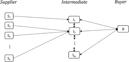
The procurement decision refers to one of the most important issues companies have to solve, to determine the optimal quantity and timing of the orders being made. Because of the difficulty and complexity of planning the material flow in a supply chain, there has been extensive research into the topic. Early studies include Wagner and Whitin (1958) who modelled the problem under single product, multi-period conditions, while later research was conducted under various conditions and with different restrictions (Bushuev et al. 2015). Another fundamental decision companies have to make is that of supplier selection, a topic that has been approached from various angles, using different methods and criteria (de Boer, Labro, and Morlacchi 2001; Wetzstein et al. 2016). It has been observed that transportation costs can make up over 50% of the total logistics costs of a product (Swenseth and Godfrey 2002). Combining all the aspects indicated above with an intricate supplier network, that includes intermediate inventory facilities, increases the complexity and with it the need for a coordinated approach. So far, studies into these topics focus mainly on supply networks with multiple origins (and sometimes destinations), paying less attention to intermediate nodes, like transshipment nodes, warehouses or consolidation points, even though that can entail considerable cost-saving opportunities (Ülkü 2009). However, this adds another layer of complexity, making it harder to determine and model optimal solutions, especially when intermodal transportation is available to the decision-maker involved. Figure 1 provides an overview of the supply-intermediate-demand network.

Figure 1. Supply and demand network with intermediate nodes.

Several studies have adopted a combined approach to the two major problems of procurement lot-sizing and supplier selection (Aissaoui, Haouari, and Hassini 2007; Liao and Rittscher 2007; Rezaei and Davoodi 2011; Rezaei et al. 2016), using mathematical programming to describe the constraints in the system. Although integrated supplier selection and procurement lot-sizing is an old and active research area, the impact of collaboration is largely overlooked in the existing literature.

The collaboration in procurement decisions can offer many advantages, especially in large networks. According to Choudhary and Shankar (2013), ‘the total logistics cost can also come down through economies of scale in the purchasing and transportation costs, and reduction in supply chain disruptions’. Applications of such models are relevant in many real-world contexts of network connections, such as in ports, transshipment terminals or cross-docking operations (Ben-Daya, Darwish, and Ertogral 2008; Bruno, Genovese, and Piccolo 2014). Industry clusters can also be regarded as appropriate areas of application for co-procurement. An industry cluster is referred to a group of similar firms in a particular field which is located in a geographically proximate region and generally involves common supplier-buyer linkages (Porter 1998). Because of their proximity, firms in an industry cluster can draw considerable benefits from collaborative procurement. The collaboration opportunities can also add value to the logistics of the physical internet, by impacting positively transportation and inventory costs, through consolidation (Venkatadri, Krishna, and Ülkü 2016).

Motivated by the benefits of collaborative procurement and the existing gap in the literature, this paper attempts to combine procurement lot-sizing and supplier selection, within a unified model, with the aim of minimising costs for the parties involved. This integrated approach makes it possible not only to optimise the supply chain planning for the parties involved, but also to examine their collaborative relationship in greater detail. A collaborative network can provide a solution for the problems involved, while economies of scale can be realised through a collaborative network (Groothedde, Ruijgrok, and Tavasszy 2005). A case study from Dutch Food Valley is introduced to investigate these benefits under practical settings. Our case study involves dairy companies (buyers) in the region which produce boxed milk and their milk carton package suppliers. Co-procurement is a largely area in supplier selection and lot-sizing. Analysing the impact of transaction costs on the optimal number of parties involved is a new approach to studying the collaboration between buyers wanting to optimise their supply chain. Determining the optimal size of the collaboration, and optimising the supply chain planning, is an important aspect that has rarely been addressed in the literature, and one that can be highly beneficial to the parties involved. Illustrating the proposed concept through a real-world case study is another significant attribute of the current research which provides a better understanding into the features of the problem.

In the next section, a mathematical model for procurement lot-sizing with multiple suppliers is formulated. In Section 3, an approach to estimating the transaction costs is proposed, after which numerical experiments of a case study are provided in Section 4, illustrating the problem, and Section 5 presents the conclusion and suggestions for future research.

2. Problem formulation

Consider a set of buyers, each of which, depending on their demand, should find the best suppliers in each given time period and find the optimal order size from each of the selected suppliers such that the buyer’s total cost is minimised. The buyers can use different modes of transport. A buyer may make this procurement decision from multiple suppliers individually or consider collaborating with the other buyers (co-procurement) where it can benefit from the intermediate facilities (for instance for consolidation purpose). While co-procurement may be beneficial, due to its economies of scale (for example through consolidation), there are some transaction costs involved, which implies that there will be an optimal number of buyers for a given co-procurement. In this section, a mathematical model is presented for the problem. The model is designed such that it represents the co-procurement case, in other words, the model could find the optimal solution under the collaboration. It is clear, however, that, if we consider only one buyer for the model, it provides the optimal solution for that particular buyer outside the collaboration, in the conventional optimisation problem.

2.1. Assumptions and notations

The following assumptions and notations are used to formulate the problem as a mathematical model.

2.1.1. Assumptions

1. Initial and final inventory levels are zero.

2. Suppliers and intermediate inventory facilities have limited supply and storage capacity for each period, respectively.

3. Buyers have independent customer segments and no competition exists among them.

4. The problem can outline buyers in a retail or production sector.

5. In the case of a production sector, the conversion rate of raw material to final product is used to transform customer demand into raw material demand and demands are shifted L periods (production lead time) backward.

6. Shortage is allowed. Demand that is not satisfied is backordered for the next period with a (predefined) percentage counting towards lost sales. Backorders are not allowed for the final period.

7. The vehicles have restricted capacity, and the number of vehicles is unlimited.

8. Suppliers have been prequalified by all buyers regarding their general characteristics such as product quality, trust, commitment, and buyer-supplier relationship.

9. The candidate buyers are preselected and eager to have long-run partnerships.

2.1.2. Notations

Indices

$i,j$	=	Indicates any node in the network ($i\ne j$)
$s$	=	Indicates the supplier node in the network
$t$	=	Indicates the time period
$m$	=	Indicates the mode of transport

Sets
$I$	=	Sets of buyers and intermediate facilities
$B$	=	Set of buyers in the network
$S$	=	Set of suppliers in the network
$Arcs$	=	Sets of arcs (connections between nodes i and j) in the network
$T$	=	Set of time intervals
$M_{i,j}$	=	Set of modes of transport available between any nodes i and j (including supplier)

Parameters
$D_i^t$	=	Constant demand in node i in time period t
$p{c}_{s,}$	=	Procurement capacity for supplier s
$p{p}_s^t$	=	Unit purchasing price of supplier s in time period t
$h{c}_i$	=	Unit holding cost for facility i per period
$o{c}_s^t$	=	Ordering cost for supplier s in time period t
$tt{c}_{i,j,m}$	=	Transportation cost of a vehicle of type m from any node i to j
$d{t}_{i,j,m}$	=	Delivery time from any node i to j using mode m
$w$	=	Inventory space that each item takes up
$i{c}_i$	=	Inventory capacity in facility i
$tr{c}_m$	=	Vehicle capacity of mode type m
${\gamma }_i$	=	Percentage of backordering (at facility i), between zero and one, corresponding to no backordering and full backordering (no lost sales) respectively
$bo{c}_i$	=	Unit penalty cost at facility i for backordering per period
$ls{c}_i$	=	Unit penalty cost at facility i for lost sales

Variables
$Z_i$	=	Binary variable, 1 if buyer i is a part of the collaboration, 0 otherwise
$X_{i,j,m}^t$	=	Number of items transported from any node i to j in time period t with mode m
$X{T}_{i,j,m}^t$	=	Number of vehicles transporting items from any node i to j in period t with mode m
$H_i^t$	=	Amount of inventory held in facility i in time period t
$Y_s^t$	=	Binary variable, 1 if supplier s is used in period t, 0 otherwise
$S_i^t$	=	Shortage at facility i in time period t
$B_i^t$	=	Backordered items at facility i in time period t
$L{S}_i^t$	=	Lost sales items at facility i in time period t

2.2. Transaction cost

When examining collaboration among buyers (co-procurement), the value of the transaction costs should be taken into account. Existing research into the topic indicates that there is no general consensus on the definition of transaction costs, in particular when assigning a specific value. For the purpose of this study, the value to be assigned is based on the number of interactions between the different parties, as indicated in the following equation: (1) $\vartheta =A\cdot \left(\frac{N\cdot \left(N-1\right)}{2}\right)$(1) where $\vartheta$ represents the transaction costs, A the average cost per interaction, and N the number of participants in the collaboration.

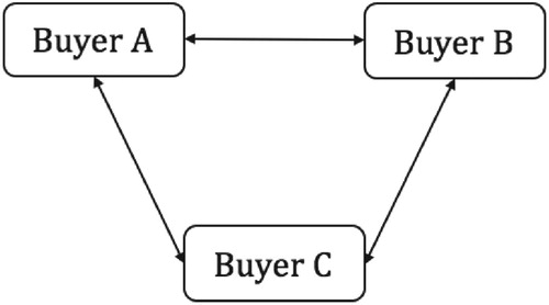
Clearly, when there are more parties involved, transaction costs increase polynomially. This is something that can be seen in reality, because when there are more parties involved, more effort (and money) is needed to maintain the proper collaboration and communication channels that are required to maintain the collaboration. Parameter A in that equation indicates at what scale the value of the transaction costs will increase based on the number of connections between parties (Figure 2).

Figure 2. An example of buyers connections.

2.3. Objective function

The objective of the model is to minimise the total costs ${\mathrm{\Pi }}_T$ for the buyers, which is defined as follows: $\begin{array}{rl}min{\mathrm{\Pi }}_T& =\text{purchasing}\text{cost}+\text{ordering}\text{cost}\\ & +\text{holding}\text{cost}+\text{transportation}\text{cost}\\ & +\text{shortage}\text{penalty}\text{cost}+\text{transaction}\text{cost}\end{array}$

The total costs relate to purchasing, ordering, holding, transportation, penalty shortage costs involved in meeting demand and transaction cost which has the following form: (2) $\begin{array}{rl}& min\sum _{t\in T}\sum _{s\in S}\left(p{p}_s^t\cdot \left(\sum _{j\in I}\sum _{m\in M_{s,j}}{X}_{s,j,m}^t\right)\right)\\ & +\sum _{t\in T}\sum _{s\in S}\left(o{c}_s^t\cdot Y_s^t\right)+\sum _{t\in T}\sum _{i\in I}\left(h{c}_i\cdot H_i^t\right)\\ & +\sum _{t\in T}\sum _{i\in I\cup S}\sum _{j\in I/i}\sum _{m\in M_{i,j}}\left(tt{c}_{i,j,m}\cdot X{T}_{i,j,m}^t\right)\\ & +\sum _{t\in T}\sum _{i\in I}\left(bo{c}_i\cdot B_i^t+ls{c}_i\cdot L{S}_i^t\right)\\ & +A\cdot \left(\frac{N\cdot \left(N-1\right)}{2}\right)\end{array}$(2)

2.4. Constraints

The following constraints are applied to the model:

2.4.1. Flow conservation constraint

This constraint expresses the flow conservation for any intermediate and demand node i in the network. It guarantees that the items left from the previous period $\left(H_i^{t-1}\right)$plus the ones which arrive at the node in current period are equal to what is currently left in inventory, plus the ones which are sent to the other nodes plus what is used to meet demand, with latter including the current demand ($D_i^t$) plus any back-orders from the previous period ($B_i^{t-1}$), minus the shortage of that period ($S_i^t$). (3) $\begin{array}{rl}& H_i^{t-1}+\sum _{j\in I{\cup }^S/i}\sum _{m\in M_{i,j}}{X}_{j,i}^{t-d{t}_{j,i,m}}\\ & =H_i^t+\sum _{j\in J/i}\sum _{m\in M_{i,j}}\left(X_{i,j,m}^t\right)+D_i^t+B_i^{t-1}-S_i^t\\ & \mathrm{\forall }t\in T,i\in I,\left(i,j\right)\in Arcs\end{array}$(3) where the variables related to the satisfaction of demand ($D_i^t+B_i^{t-1}-S_i^t$) are only applied to the constraint when node i corresponds to the buyer (demand) node. If it does not, these variables are excluded from the constraint.

The model accounts for a variable transportation time between nodes and modes $\left(d{t}_{i,j,m}\right)$, while allowing for a diversity in the way the nodes are arranged and connected in the network (using the set $Arcs$).

2.4.2. Ordering costs constraint

This constraint serves a dual purpose in the model, first to ensure that the ordering costs are taken into account $\left(Y_s^t\right)$, when a buyer places an order at supplier s, which relates to the fixed part of the ordering costs, while the second function of this constraint is designed to guarantee that the procurement capacity for supplier s is not exceeded, but stay within the limits set by parameter $p{c}_s$. (4) $\sum _{j\in I}\sum _{m\in M_{s,j}}{X}_{s,j,m}^t\le p{c}_s\cdot Y_s^t\mathrm{\forall }t\in T,s\in S$(4)

2.4.3. Non-admissible flow constraint

These constraints express that the flow between a buyer and intermediate facilities as well as other buyers is admissible only if that buyer is a part of collaborative procurement which is indicated by $Z_i$. In other words, a buyer can benefit from consolidation of flows in the case that it is involved in collaboration. (5) $\begin{array}{rl}& \sum _{j\in I}\sum _{m\in M_{i,j}}{X}_{i,j,m}^t\le M_1.Z_i\mathrm{\forall }t\in T,i\in B\end{array}$(5) (6) $\begin{array}{rl}& \sum _{j\in I}\sum _{m\in M_{i,j}}{X}_{j,i,m}^t\le M_2.Z_i\mathrm{\forall }t\in T,i\in B\end{array}$(6) where M₁ and M₂ are sufficiently large numbers.

2.4.4. Collaboration size constraint

The number of participants in the collaboration (N) is obtained as follows: (7) $N=\sum _{i\in B}{Z}_i$(7)

2.4.5. Inventory limitations constraint

This constraint relates to the inventory limits being set for each facility i. Like the previous constraint, this constraint also ensures that the quantity of items left for storage $\left(H_i^t\right)$, multiplied by their volume, does not exceed the facility’s storage space. (8) $w\cdot H_i^t\le i{c}_i\mathrm{\forall }t\in T,i\in I$(8)

2.4.6. Vehicle capacity limitation constraint

This constraint ensures that the number of vehicles that are used on the route between facilities i and j are the ones required to transport the products for period t. More specifically, the cumulative volume of the products, divided by capacity of the vehicles, indicates the minimum number of required vehicles of that type. (9) $\begin{array}{rl}& \frac{w\cdot X_{i,j,m}^t}{tr{c}_m}\le X{T}_{i,j,m}^t,\\ & \mathrm{\forall }t\in T,m\in M_{i,j},i\in I{\cup }^S,j\in I/i,\left(i,j\right)\in Arcs\end{array}$(9) This constraint allows for consolidation of items being transported on the same route, allowing for cost-cutting opportunities, by increasing the utilisation of the vehicles.

2.4.7. Backorders and lost-sales assignment constraint

These constraints ensure that backorders are assigned the appropriate integer values, based on the percentage $\left(\gamma \right)$, and that the remaining quantity is considered to be lost sales. Constraint (10) allows variable $B_i^t$ to obtain integer values, by restricting it inside $\left[\gamma \cdot S_i^t\dots \gamma \cdot S_i^t+1\right]$ which is quarantined to contain an integer value. Constraint (11) assigns values to lost sales, based on shortage and backorders. (10) $\begin{array}{rl}& \gamma \cdot S_i^t\le B_i^t<\gamma \cdot S_i^t+1\mathrm{\forall }t\in T,i\in I\end{array}$(10) (11) $\begin{array}{rl}& S_i^t=B_i^t+L{S}_i^t\mathrm{\forall }t\in T,i\in I\end{array}$(11)

2.4.8. Initialisation and final period constraints

Constraints (12) and (13) ensure that there is no inventory for the first and last period for all facilities, although they could be modified and given initial or final values, as required. Constraints (14) and (15) ensure that there are no back-orders for the first and last time periods. (12) $\begin{array}{rl}& H_i^0=0\mathrm{\forall }i\in I\end{array}$(12) (13) $\begin{array}{rl}& H_i^T=0\mathrm{\forall }i\in I\end{array}$(13) (14) $\begin{array}{rl}& B_i^0=0\mathrm{\forall }i\in I\end{array}$(14) (15) $\begin{array}{rl}& B_i^T=0\mathrm{\forall }i\in I\end{array}$(15)

2.4.9. Binary, and non-negativity constraints

The following constraints ensure that the variables can only be assigned the appropriate positive (or binary) values. (16) $\begin{array}{rl}& Y_s^t\in \left\{0,1\right\}\mathrm{\forall }t\in T,s\in S\end{array}$(16) (17) $\begin{array}{rl}& Z_i\in \left\{0,1\right\}\mathrm{\forall }i\in B\end{array}$(17) (18) $\begin{array}{rl}& X_{i,j,m}^t,X{T}_{i,j,m}^t\ge 0,Int\mathrm{\forall }t\in T,i\in I\cup S,j\in I,m\in M_{i,j}\end{array}$(18) (19) $\begin{array}{rl}& H_i^t,S_i^t,B_i^t,L{S}_i^t\ge 0,Int\mathrm{\forall }t\in T,i\in I\end{array}$(19)

The proposed model is a centralised optimisation scheme which specifies the most cost efficient collaboration structure i.e. involved buyers and their collaborative decisions as well as the decisions of buyers which are out of the collaboration. The model is solved for each buyer individually by eliminating all other nodes of buyers and intermediate facilities and removing the transaction costs. The optimal cost for buyer k, when the model is solved for that buyer individually, is called ${\mathrm{\Pi }}_k^{\ast }$. The optimal cost for buyer k, when the model is solved under co-procurement is called ${\mathrm{\Pi }}_k^{Co}$, which is calculated as follows: (20) ${\mathrm{\Pi }}_k^{Co}={\mathrm{\Pi }}_T^{\ast }\left(\frac{{\mathrm{\Pi }}_k^{\ast }}{{\sum }_{i\in K}{\mathrm{\Pi }}_i^{\ast }}\right)$(20) where ${\mathrm{\Pi }}_T^{\ast }$is the optimal total cost of the system. Equation (20) indicates that the total cost of the system is distributed among the parties based on their cost contribution in the individual setting. This is one of the prevalent cost-sharing schemes in the centralised and collaborative structures which can be done via coordination mechanisms (e.g. a formal contract) (Giannoccaro and Pontrandolfo 2004). The proposed scheme guarantees that even the buyers which are kept out of collaboration in the centralised optimisation model, will benefit by experiencing a cost reduction which is a key point in long-run partnerships (this is because ${\mathrm{\Pi }}_T^{\ast }\le \sum _{i\in K}{\mathrm{\Pi }}_i^{\ast }$).

3. Computational results

The performance of the proposed collaborative procurement scheme is illustrated through a case study applied to a food industry cluster in the Netherlands which is known as Dutch Food Valley. As the objective function is convex and the constraints are linear, the problem is one of integer quadratic programming for which unique optimal solution exists if the solution space is feasible (Chaovalitwongse, Androulakis, and Pardalos 2009). The model belongs to the class of NP-hard problems (Del Pia, Dey, and Molinaro 2017) for which the computational complexity increases sharply as the size of the problem gets larger. Accordingly, a sufficiently sized instance is used for our case study which is able to showcase the full extent of the model discussed above. The computations start by focusing on a single buyer and are then expanded to include collaboration of buyers to optimise their costs. Additionally, the value of the transaction costs involved is examined in greater detail, to see how this can alter the number of collaborators involved, in order to maintain the preferred cost-savings.

The model is coded in IBM ILOG CPLEX Optimisation Studio 12.7 and the experiments are carried out on a computer with Intel® Core i7-8650U CPU 1.9, 2.11 GHz, and 7.88 GB memory available.

3.1. Case study

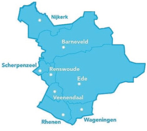
The agri-food industry is one of the key drivers of the economy in the Netherlands, which is the second biggest exporter of food worldwide. Dutch Food Valley is an important food industry cluster in the Netherlands where Dutch and international food companies and research institutes are concentrated. It is located in lower Rhine Valley with the city of Wageningen as its core, embracing the municipalities of Nijkerk, Barenveld, Scherpenzed, Renswoude, Veenedaal, Rhenen and Ede. The region is in the midst of major highways, railroads and water transport routes. Figure 3 depicts the geographic illustration of the region.

Figure 3. Graphic illustration of Dutch Food Valley.

Our case study investigates dairy companies (buyers) in the region, which produce boxed milk, and their milk carton package suppliers. Figure 4 illustrates the network structure of this problem.

Figure 4. Network structure.

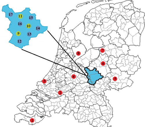
The network involves eight suppliers (nodes 1:8), three intermediate facilities (nodes 9:11) and six buyers (nodes 12:17). All the nodes are interconnected, and items can be transported between the nodes, using the available modes. The planning horizon involves 6 periods and 2 modes of transport are available including city-delivery trucks with the capacity of 18 m³ and larger trucks with the capacity of 32 m³. These are experimental choices which can fully depict the features of the problem; the proposed structure can be used for problems with other sizes.

The intermediate facilities can be used as warehouses and/or as consolidation terminals. It must also be noted that the buyers (dairy companies) can act both as intermediates and as demand nodes, which implies that a buyer is permitted to receive amounts more than its own demand, where the extra amount is then transported to the other nodes (intermediate nodes or other collaborating buyers). Accordingly, the arcs from the suppliers to the buyers and intermediate nodes are unidirectional, while the arcs between the buyers and the intermediate nodes are bidirectional.

Each milk carton is used as the package for one litre boxed milk ($\eta =1$) which is filled by the buyer. The time of this process is assumed to be negligible in comparison to the period length (one week). One unit of product involves a batch size of 12 milk package cartons at the supplier and 12 filled milk boxes at the buyer and each batch of package cartons occupies 0.018 m³. Table 1 shows the unit purchasing price ($p{p}_s^t$) and the ordering cost ($o{c}_s^t$) for each one of the suppliers. It is assumed that these prices do not vary over time.

Table 1. Purchasing price and ordering cost per supplier.

Supplier	Purchasing price	Ordering cost
1	4.2	250
2	3.8	260
3	3.8	230
4	3.6	240
5	3.6	260
6	4.4	240
7	4.1	280
8	4	220

Table 2 indicates the demand of each buyer ($d{d}_i^t$).

Table 2. Demand for each buyer at each period.

	Time period
Buyer	1	2	3	4	5	6
12	980	1000	1020	1020	1040	1060
13	1070	960	1120	1130	1140	1150
14	1020	1020	1080	840	1110	1120
15	970	960	970	970	1000	1020
16	1010	970	1060	1010	1080	1100
17	1010	1040	1090	1080	1100	1110

The holding costs for all intermediate storage facilities $\left(hc\right)$ is 1 per item stored for a single time period. The total storage space for these facilities $\left(i{c}_i\right)$ is limited to 1000 m³. A backordering ratio $\left({\gamma }_i\right)$ of 1 is considered (100% of shortage is backordered at no lost sales). The backordering penalty cost $\left(bo{c}_i\right)$ of each buyer is 1.2 per item for a single time period.

The transportation costs ($tt{c}_{i,j,m}$) is calculated based on the distance between the different nodes in the network which are provided in Table 3. Since the network entities are located in relatively close proximity to each other, it is considered that transportation time ($d{t}_{i,j,m}$) is negligible in comparison to the period length.

Table 3. Relevant distances (per kilometre) between the different nodes in the network.

(i,j)	1	2	3	4	5	6	7	8	9	10	11	12	13	14	15	16	17
1	–	–	–	–	–	–	–	–	215	228	227	211	228	239	230	234	223
2	–	–	–	–	–	–	–	–	89.5	109	101	85	102	113	104	108	97
3	–	–	–	–	–	–	–	–	107	112	111	113	112	115	116	118	107
4	–	–	–	–	–	–	–	–	48	53.4	52	54	53.2	56	55	60	48
5	–	–	–	–	–	–	–	–	94.5	96	116	90	90	91	117	113	117
6	–	–	–	–	–	–	–	–	71	53	53	68	64	55	56	61	48
7	–	–	–	–	–	–	–	–	101	82.6	82.7	98	93.5	85	86	90.7	68.3
8	–	–	–	–	–	–	–	–	128	123	108	134	129	126	111	112	88
9	–	–	–	–	–	–	–	–	–	15.3	24.8	7.1	11.2	18.3	25.6	21.3	33.8
10	–	–	–	–	–	–	–	–	15.3	–	19.8	21.8	4.7	5.2	18	16.3	28.8
11	–	–	–	–	–	–	–	–	24.8	19.8	–	31.4	25.8	23.4	6.7	8.7	11.3
12	–	–	–	–	–	–	–	–	7.1	21.8	31.4	–	14	27	32.2	27.8	40.3
13	–	–	–	–	–	–	–	–	11.2	4.7	25.8	14	–	6.4	24.3	20	32.5
14	–	–	–	–	–	–	–	–	18.3	5.2	23.4	27	6.4	–	22	19.3	31.8
15	–	–	–	–	–	–	–	–	25.6	18	6.7	32.2	24.3	22	–	8.5	16.6
16	–	–	–	–	–	–	–	–	21.3	16.3	8.7	27.8	20	19.3	8.5	–	12.5
17	–	–	–	–	–	–	–	–	33.8	28.8	11.3	40.3	32.5	31.8	16.6	12.5	–

3.2. Results (individual)

In this section, the results are analysed from the perspective of single buyers. Suppliers 3, 4 and 5 are the selected ones in the problem where supplier 3 serves buyers 16 and 17, supplier 4 serves buyers 12 and 13 and supplier 5 serves buyers 14 and 15. For the sake of brevity, the detailed replenishment decisions are represented only for buyers 15 and 16 which are provided in Tables 4 and 5, respectively.

Table 4. Replenishment decisions for buyer 15.

	$X_{5,15,m}^t$
Time Period	$m=1$	$m=2$	$H_{15}^t$	$B_{15}^t$
1	970	0	0	0
2	960	0	0	0
3	970	0	0	0
4	990	0	20	0
5	1000	0	20	0
6	1000	0	0	0

Table 5. Replenishment decisions for buyer 16.

	$X_{3,16,m}^t$
Time period	$m=1$	$m=2$	$H_{16}^t$	$B_{16}^t$
1	1000	0	0	10
2	980	0	0	0
3	0	1070	10	0
4	1000	0	0	0
5	0	1180	100	0
6	1000	0	0	0

Vehicle mode 2 is only used when the capacity of the first mode is not sufficient to meet the demand which is completely expected as the transportation costs of the second mode are higher. As the results project, the excess inventory and backorders are mostly avoided to reduce the costs. As an instance, backorder occurs in the system of buyer 16 only in period 1 so that the demanded items can be carried by mode 1 which is cheaper. Similarly, excess inventory is held only for periods 3 and 5 so that the demand for subsequent period is met by using mode 1 for delivery.

The total cost of each buyer and its constituent elements are provided in Table 6.

Table 6. Costs per buyer.

Buyer	Total cost	Purchasing cost	Ordering cost	Holding cost	Transportation cost	Backordering penalty cost
12	26,236	22,032	1440	120	2644	0
13	28,186	23,652	1440	0	3094	0
14	27,607	21,665	1560	406	3976	0
15	26,437	20,615	1560	52	4210	0
16	29,640	29,640	1380	165	4948	96
17	30,235	30,235	1380	432	4552	80
Sum	168,341	147,839	8760	1175	23,424	176

As Table 6 depicts, purchasing cost, transportation cost and ordering cost are the three largest cost components, respectively.

In the next subsection, multiple buyers are involved in the decision-making process. The results are used to show the improvement in costs that are made possible by a more collaborative approach to the problem being solved.

3.3. Results (co-procurement)

In this section, the mathematical model discussed in Section 2 is used, with the discussed experimental case study.

Again suppliers 3, 4 and 5 are selected to serve the demand points. The optimal size of the collaboration is four with buyers 13, 14, 15 and 16. They jointly use node 10 as their intermediate inventory node to facilitate collaboration. If we take a relook at Figure 4, the results can be easily justified by the topology of these nodes. Expressly, buyers 13–16 are in closer proximity of each other and the intermediate facility 10 is located between them.

We take buyers 15 and 16 to have a closer look at the results. In the collaborative setting, no excess inventory or backorders have occurred for these two buyers and 590 items are held in intermediate facility 10 in period one. The flow of products for these two buyers and the intermediate facility 10 is depicted in Figure 5 (dotted arrows represent vehicle mode 1).

Figure 5. Network flow for buyers 15 and 16.

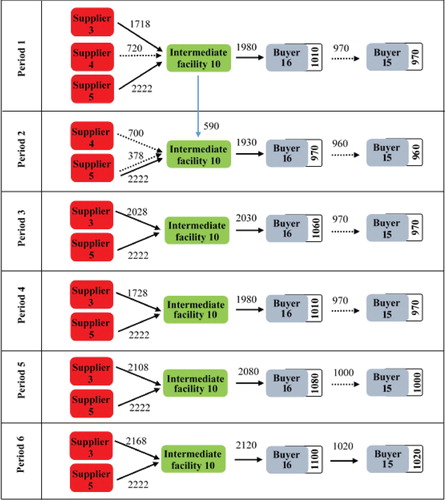
It can be seen that for consolidation purposes, a large number of items passed through the intermediate facility 10, and from there were transferred to their final destinations. Precisely, from 37,420 demanded items of all the buyers in the planning horizon, 68% are passed through intermediate facility 10 and the remainder is directly transferred from the suppliers to their final destinations. The total cost of the system is 153,639 monetary units which is reduced by 14,703 in comparison to non-collaborative setting. The value of the cost components and their reduction in comparison to non-collaborative case are shown in Table 7.

Table 7. Cost components.

	Total cost	Purchasing cost	Ordering cost	Holding cost	Transportation cost	Backordering penalty cost	Transaction cost
Value	153,639	136,698	4150	385	10,504	102	1800
Reduction	14,703	11,141	4610	790	12,920	74	–

By switching to co-procurement, the ordering cost undergoes a 52% decrease as the buyers pay one ordering fee for consolidated orders. This, in turn, provides each buyer with the chance to purchase from more than one supplier if the order size exceeds the remaining capacity of the suppliers. So, larger orders enter the system of the suppliers with lower prices which decreases the purchasing cost of the system by 7.5%. Consolidation of orders and using the intermediate inventory facilities effectively lowers the transportation cost by 55%. All in all, the benefits of the co-procurement stem from the savings in firstly, transportation, then ordering and finally purchasing costs.

Total cost of each buyer and its saving in comparison to individual setting are provided in Table 8:

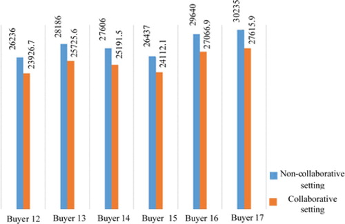
Table 8. Costs per buyer.

Buyer	Total cost	Savings from collaboration (%)
12	23,926.7	8.6
13	25,725.63	8.7
14	25,191.48	8.75
15	24,112.12	8.8
16	27,066.98	8.7
17	27,615.89	8.65
Sum	153,638.8	8.7

As the results convey, all of the buyers benefit by a reduction in their cost in collaborative setting which emphasises the positive impact of co-procurement. The savings (in percentage) provided by collaboration are relatively equal for the buyers which shows the efficiency of the proposed cost-sharing mechanism. To compare these costs with the ones in non-collaborative setting, Figure 6 is provided.

Figure 6. Comparison of costs in collaborative and non-collaborative setting.

3.4. Sensitivity analysis

A sensitivity analysis was performed to see how fluctuations in the values of the transaction costs can affect the results. The transaction costs are stretched from the initial values, to see the shift in the optimal number of collaborators and the optimal total cost; the results of which are provided in Table 9.

Table 9. Sensitivity analysis on transaction cost.

Changes (%)	Collaboration size	Total cost
−100	6	147,314 (−4.2%)
−50	5	150,110 (−2.29%)
0	4	153,639
+50	4	154,539 (+58%)
+100	3	158,079 (+2.88%)
+150	2	161,701 (+5.24%)
+200	2	162,601 (+5.83%)
+250	2	163,501 (+6.41%)
+300	1	168,341 (+9.6%)

Figure 7 depicts the optimal collaboration size with respect to changes in transaction cost graphically.

Figure 7. Sensitivity analysis on transaction cost.

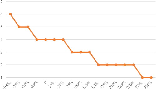
It can be seen that the optimal size for a collaboration changes as the transaction cost varies. The total cost of the system also shifts when transaction cost increases, as was expected. When the transaction costs decrease, the size of collaboration increases, such that if, for instance, we have a reduction of 100%, the size of collaboration would be 6, which implies that the total system benefits most if each buyer collaborates with all the other 5 buyers. On the other hand, if we increase the transaction costs significantly buyers prefer to collaborate with no other buyer (the size is 1 which indicates no collaboration). The calculations show that there exist specific intervals of transaction costs in between these extremes, under which the optimal collaboration size remains unchanged. This indicates that the number of partners is robust for changes in transaction costs, up to 25–50%.

4. Discussion

In this section, a case study was introduced, implementing the mathematical model that was discussed in Section 2. The cased involved six different buyers wanting to optimise their costs. Individual costs when working independently can be decreased further by collaborating with other buyers, which provides cost-saving opportunities through economies of scale. Even when transaction costs are involved, there are opportunities for decreased cost. However, the optimal size of a collaboration will change considerably depending on the value of these costs. For the case discussed here, the optimal size of a collaboration was found to be located at four buyers which were in closer proximity to each other. The differences in demand and location of each buyer leads to differences in cost savings through co-procurement. The results indicated that the savings in firstly, transportation, then ordering and finally purchasing costs are higher than savings in other cost components. The sensitivity analysis that was performed showed that the results are sensitive to the changes in the value of the transaction costs, meaning that by trying to reduce the transaction costs, the buyers are willing to collaborate with more buyers as this is in their financial benefits.

5. Conclusion and future work

In this study, a number of fundamental problems facing most buyers, including procurement lot-sizing from multiple suppliers, and transportation network complexity, were considered simultaneously. A mathematical model was formulated to integrate and solve these problems. The optimal solution resulting from the joint problem indicates the optimal lot-sizing (which quantities, with which supplier, in which periods), as well as mode selection and intermediate storage facilities, in order to minimise the total costs. Using an integrated approach to address these problems can yield multiple benefits. For instance, most procurement models do not incorporate complex transportation networks, with multiple levels of intermediate facilities and modes. An integrated approach makes it possible to tackle all these problems simultaneously and increase the available cost-saving opportunities.

The mathematical formulation that was proposed is a stepping stone in examining the cost-savings that a collaboration between buyers, called co-procurement, can yield. The model can determine optimal collaboration size and the parties working together, making it possible to examine these relations more closely. Approximating the transaction costs of this collaboration was a significant aspect, to which existing literature thus far has not assigned a specific value. By incorporating the modelling approach and the transaction cost for a variable combination of buyers, it is possible to estimate the cost-savings of these collaborations. The proposed structure was illustrated through a case study from Dutch Food Valley to investigate the benefits of co-procurement under practical settings. The results indicate that co-procurement can bring considerable cost-savings through consolidation of orders and more efficient transportation schedules. Collaboration in procurement can also effectively handle disruptions that easily impact the supply chain performance of the involved buyers and thereby increase the resilience against the ripple effect (Dolgui, Ivanov, and Sokolov 2018). As a common instance, if a supplier encounters a problem in meeting the orders of its buyers in the individual setting, the buyers will face non-anticipated shortages and unsatisfied customers which can lead to a market loss. In the case of collaboration, these orders can be satisfied by the excess products in intermediate facilities and (or) surrounding buyers within a contractual agreement.

Based on the findings of this study, several recommendations can be made for future research. The mathematical model proposed in this study integrates a number of decisions in an effort to identify the optimal costs. For future research, the objective function could be modified to include environmental aspects like carbon emissions. The availability for intermodal transportation provided by the proposed models would allow for the consideration of emission reductions, as a multi-objective problem that also addresses the effort by many companies to reduce emissions in relation to their supply network, such as in (Baykasoglu and Subulan 2016). Further research can also focus on collaboration costs, as well as sharing of costs and benefits, possibly involving game theory, to gain a more in-depth perspective of the complex behaviour that is involved in collaborations, where different entities benefit in varying degrees(Cachon and Netessine 2004). These benefits can vary, based on a number of parameters that can also be investigated, such as the location of the buyers, which can heavily influence the potential gains from a collaboration effort. Although a game-theoretic approach to collaboration has been examined and analysed, as a means to reduce product development costs (Arsenyan, Buyukozkan, and Feyzioglu 2015), this approach can be extended to involve collaboration on a greater scale involving parties that will cooperate in order to reduce the overall supply chain costs. Developing an efficient solution algorithm for the problem which would be able to solve large size instances in reasonable time is another promising future direction for this study.

Disclosure statement

No potential conflict of interest was reported by the author(s).

References

- Aissaoui, N., M. Haouari, and E. Hassini. 2007. “Supplier Selection and Order Lot-Sizing Modeling: A Review.” Computers & Operations Research 34 (12): 3516–3540. doi: 10.1016/j.cor.2006.01.016
- Arsenyan, J., G. Buyukozkan, and O. Feyzioglu. 2015. “Modeling Collaboration Formation with a Game Theory Approach.” Expert Systems with Applications 42 (4): 2073–2085. doi: 10.1016/j.eswa.2014.10.010
- Baykasoglu, A., and K. Subulan. 2016. “A Multi-Objective Sustainable Load Planning Model for Intermodal Transportation Networks with a Real-Life Application.” Transportation Research Part E: Logistics and Transportation Review 95 (2016): 207–247. doi: 10.1016/j.tre.2016.09.011
- Ben-Daya, M., M. Darwish, and K. Ertogral. 2008. “The Joint Economic Lot-Sizing Problem: Review and Extensions.” European Journal of Operational Research 185 (2): 726–742. doi: 10.1016/j.ejor.2006.12.026
- Bruno, G., A. Genovese, and C. Piccolo. 2014. “The Capacitated Lot Sizing Model: A Powerful Tool for Logistics Decision Making.” International Journal of Production Economics 155: 380–390. doi: 10.1016/j.ijpe.2014.03.008
- Bushuev, M. A., A. Guiffrida, M. Y. Jaber, and M. Khan. 2015. “A Review of Inventory Lot Sizing Review Papers.” Management Research Review 38 (3): 283–298. doi: 10.1108/MRR-09-2013-0204
- Cachon, G. P., and S. Netessine. 2004. “Game Theory in Supply Chain Analysis.” In Handbook of Quantitative Supply Chain Analysis, edited by D. Simchi-Levi, David Wu, and Max Shen, 13–65. New York: Kluwer.
- Chaovalitwongse, W. A., I. P. Androulakis, and P. M. Pardalos. 2009. “Quadratic Integer Programming: Complexity and Equivalent Forms”. In Encyclopedia of Optimization, edited by C. Floudas and P. Pardalos. Boston, MA: Springer.
- Choudhary, D., and R. Shankar. 2013. “Joint Decision of Procurement Lot-Size, Supplier Selection, and Carrier Selection.” Journal of Purchasing & Supply Management 19 (2013): 16–26. doi: 10.1016/j.pursup.2012.08.002
- de Boer, L., E. Labro, and P. Morlacchi. 2001. “A Review of Methods Supporting Supplier Selection.” European Journal of Purchasing and Supply Management 7 (2): 75–89. doi: 10.1016/S0969-7012(00)00028-9
- Del Pia, A., S. S. Dey, and M. Molinaro. 2017. “Mixed-Integer Quadratic Programming is in NP.” Mathematical Programming 162 (1–2): 225–240. doi: 10.1007/s10107-016-1036-0
- Dolgui, A., D. Ivanov, and B. Sokolov. 2018. “Ripple Effect in the Supply Chain: An Analysis and Recent Literature.” International Journal of Production Research 56 (1–2): 414–430. doi: 10.1080/00207543.2017.1387680
- Dyer, J. H. 1997. “Effective Interim Collaboration: How Firms Minimize Transaction Costs and Maximise Transaction Value.” Strategic Management Journal 18 (7): 535–556. doi: 10.1002/(SICI)1097-0266(199708)18:7<535::AID-SMJ885>3.0.CO;2-Z
- Giannoccaro, I., and P. Pontrandolfo. 2004. “Supply Chain Coordination by Revenue Sharing Contracts.” International Journal of Production Economics 89 (2): 131–139. doi: 10.1016/S0925-5273(03)00047-1
- Groothedde, B., C. Ruijgrok, and L. Tavasszy. 2005. “Towards Collaborative, Intermodal Hub Networks a Case Study in the Fast Moving Consumer Goods Market.” Transportation Research Part E: Logistics and Transportation Review 41: 567–583. doi: 10.1016/j.tre.2005.06.005
- Gulati, R., N. Nohria, and A. Zaheer. 2000. “Strategic Networks.” Strategic Management Journal 21 (3): 203–215. doi: 10.1002/(SICI)1097-0266(200003)21:3<203::AID-SMJ102>3.0.CO;2-K
- Lambert, D. 2008. Supply Chain Management: Processes, Partnerships, Performance. Sarasota, Florida: Supply Chain Management Institute.
- Liao, Z., and J. Rittscher. 2007. “Integration of Supplier Selection, Procurement Lot Sizing and Carrier Selection Under Dynamic Demand Conditions.” International Journal of Production Economics 107 (2): 502–510. doi: 10.1016/j.ijpe.2006.10.003
- Martínez-Olvera, C., and Y. A. Davizon-Castillo. 2015. “Modeling the Supply Chain Management Creation of Value – a Literature Review of Relevant Concepts.” In Applications of Contemporary Management Approaches in Supply Chains, edited by H. Tozan and A. Erturk, 57–82. Rijeka, Croatia: InTech.
- Porter, M. E. 1998. Clusters and the New Economics of Competition (Vol. 76). Boston, MA: Harvard Business Review.
- Ramanathan, U., and A. Gunasekaran. 2014. “Supply Chain Collaboration: Impact of Success in Long-Term Partnerships.” International Journal of Production Economics 147: 252–259. doi: 10.1016/j.ijpe.2012.06.002
- Rezaei, J., and M. Davoodi. 2011. “Multi-Objective Models for Lot-Sizing with Supplier Selection.” International Journal of Production Economics 130 (1): 77–86. doi: 10.1016/j.ijpe.2010.11.017
- Rezaei, J., M. Davoodi, L. Tavasszy, and M. Davarynejad. 2016. “A Multi-Objective Model for Lot-Sizing with Supplier Selection for an Assembly System.” International Journal of Logistics Research and Applications 19 (2): 125–142. doi: 10.1080/13675567.2015.1059411
- Swenseth, S. R., and M. Godfrey. 2002. “Incorporating Transportation Costs Into Inventory Replenishment Decisions.” International Journal of Production Economics 77 (2): 113–130. doi: 10.1016/S0925-5273(01)00230-4
- Ülkü, M. A. 2009. Analysis of Shipment Consolidation in the Logistics Supply Chain. Waterloo: University of Waterloo.
- Venkatadri, U., K. S. Krishna, and M. A. Ülkü. 2016. “On Physical Internet Logistics: Modeling the Impact of Consolidation on Transportation and Inventory Costs.” IEEE Transactions on Automation Science and Engineering 13 (4): 1517–1527. doi: 10.1109/TASE.2016.2590823
- Wagner, H. M., and T. M. Whitin. 1958. “Dynamic Version of the Economic Lot-Size Model.” Management Science 5: 89–96. doi: 10.1287/mnsc.5.1.89
- Wetzstein, A., E. Hartmann, W. C. Benton Jr, and N. Hohenstein. 2016. “A Systematic Assessment of Supplier Selection Literature–State-of-the-art and Future Scope.” International Journal of Production Economics 182: 304–323. doi: 10.1016/j.ijpe.2016.06.022
- Williamson, O. E. 1979. “Transaction-Cost Economics: The Governance of Contractual Relations.” The Journal of Law and Economics 22 (2): 233–261. doi: 10.1086/466942
- Williamson, O. E. 1989. “Transaction Cost Economics.” Handbook of Industrial Organization 1: 135–182. doi: 10.1016/S1573-448X(89)01006-X