Rule based workload control in semiconductor manufacturing revisited

Abstract

An essential task in manufacturing planning and control is to determine when to release orders to the shop floor. A prominent approach is the workload control (WLC) concept which originated from the idea of controlling flow times by controlling order releases. Despite recent advances in rule based WLC models, the recent semiconductor literature has neglected them, although it has been shown that they outperform most other periodic and continuous order release models. Therefore, we adapt the most successful rule based WLC model, the LUMS-COR approach and compare it with two approaches from the semiconductor manufacturing literature: Starvation Avoidance (SA) and ConLOAD approach. We include three pool sequencing rules, namely First-Come First-Served (FCFS), Earliest Due Date (EDD) and Critical Ratio (CR). We analyse their performance using a simulation model of a scaled-down wafer fabrication facility. The results show that, in comparison to the other two order release approaches, the LUMS-COR model yields lower total costs due to a more balanced shop and better timing performance which is robust across different settings. This suggests that the adapted LUMS-COR model has high potential to become a viable alternative to the rule based order release mechanisms used in semiconductor industry to date.

Keywords:

• Production planning
• workload control
• order release
• simulation
• pool sequencing

1. Introduction

This paper re-examines the use of rule based workload control (WLC) in semiconductor manufacturing given the recent developments in WLC research. WLC originated from the idea of controlling flow times by controlling order releases, and thus the level of work-in-process (WIP) and output (Kingsman, Tatsiopoulos, and Hendry 1989; Wiendahl 1995). An order release model has to decide which orders should be released from an order pool to the shop floor, where the order pool contains all unreleased orders and seeks to smooth out fluctuations in the incoming flow of orders. Within the WLC literature, two streams of research can be identified (Puergstaller and Missbauer 2012; Haeussler and Netzer 2019): (i) Rule based and (ii) optimisation based order release models. The latter models formulate a multi-period optimisation model to determine the optimal order release quantities over a certain planning horizon (Missbauer and Uzsoy 2011) and have been tested in the semiconductor manufacturing context (Kacar, Irdem, and Uzsoy 2012; Kacar, Moench, and Uzsoy 2013; Ziarnetzky et al. 2015). The second category are rule-based order release mechanisms that determine when to release orders by employing a set of rules based on a variety of design options (Bergamaschi et al. 1997) and parameter settings (e.g. workload norm) of the order release mechanisms (Glassey and Resende 1988; Wiendahl 1995; Land 2004). The focus of this paper is on the latter category.

Rule based order release methods can be divided into two groups according to when the order release decision takes place: at periodic intervals or continuously (Fowler, Hogg, and Mason 2002; Thuerer et al. 2014a). When applying rule based order release models to semiconductor manufacturing, mainly continuous models were used. These approaches release new orders at any moment in response to a trigger event, i.e. the workload falling below a critical level. Methods differ from each other with regard to how the workload is aggregated, and can be either bottleneck based (Goldratt and Cox 1986; Goldratt and Fox 1986; Glassey and Resende 1988; Wein 1988; Glassey, Shanthikumar, and Seshadri 1996) or shop load based (Spearman, Woodruff, and Hopp 1990; Lin and Lee 2001). However, despite recent developments in the rule based WLC literature which mainly focuses on Small and Medium Enterprises (SME) in Make-To-Order (MTO) environments (Oosterman, Land, and Gaalman 2000; Thuerer et al. 2012, 2014a; Thuerer and Stevenson 2016; Yan et al. 2016), most recent papers on semiconductor manufacturing focus on multi-period optimisation models for order release (Kacar, Irdem, and Uzsoy 2012; Kacar, Moench, and Uzsoy 2013; Ziarnetzky et al. 2015). This might be due to findings of earlier comparative papers that show that periodic order release models are outperformed by continuous mechanisms (Hendry and Wong 1994; Sabuncuoglu and Karapınar 1999), but a recent study of Thuerer et al. (2012) shows that a hybrid approach combining periodic and continuous elements, namely the LUMS-COR (Lancaster University Management School – Corrected Order Release) model outperforms all other tested order release approaches.

Since the semiconductor wafer fab environment, with high uncertainty, long re-entrant process routings, and combination of batch and unit processing machines constitutes a very challenging environment for workload control methods, it is worth studying it from the point of view of WLC also. In this regard, as recent research on semiconductor manufacturing has not taken advantage of some of the latest developments in the WLC literature, in particular the LUMS-COR method introduced in Thuerer et al. (2012), this papers' contribution is twofold: First, it links two largely separately developed streams of research and second it analyses whether an adapted LUMS-COR approach improves the performance of rule based WLC approaches in semiconductor wafer fabs. This should serve as decision support for practitioners whether implementing the LUMS-COR model for order release is worth the effort in the semiconductor environment. Therefore, we compare the continuous Starvation Avoidance (SA) approach of Glassey and Resende (1988) and the continuous CONstant LOAD (ConLOAD) approach of Rose (1999) with an adapted LUMS-COR model (Thuerer et al. 2012), which combines continuous and periodic release elements, using a simulation model of a scaled-down wafer fabrication facility (Kayton et al. 1997).

ConLOAD was introduced to overcome the shortcoming of ConWIP (Spearman, Woodruff, and Hopp 1990) which only controls the number of jobs on the shop floor, while ConLOAD was designed to track the load situation of the fab and thus the desired and current product mix by considering the load contribution of a job to the bottleneck work centre (Rose 1999; Mönch, Fowler, and Mason 2013). SA was developed for high volume, low mix environments, while LUMS-COR was explicitly designed for a Make-To-Order, high mix environment. Although the number of such environments in wafer fabrication was quite limited about thirty years ago, it is, with the growth of the foundry model for semiconductor manufacturing, much more relevant today. Since ConLOAD and SA put their emphasis on controlling the bottleneck workload we changed the LUMS-COR approach of Thuerer et al. (2012) accordingly to yield a fair comparison. Moreover, since previous research on semiconductor wafer fabs has neglected pool sequencing rules, another contribution of this paper is the consideration of such rules in the semiconductor domain. Therefore, each of the above order release approaches is combined with First-Come First-Served (FCFS), Earliest Due Date (EDD) and Critical Ratio (CR) based pool sequencing. Performance is measured in three respects: By capturing costs, timing and load balancing measures.

The remainder of this paper is structured as follows: Section 2 reviews the relevant literature regarding rule based periodic and continuous order release models and their application domains. Section 3 outlines the used pool sequencing and order release approaches and in Section 4 we describe the simulation model and the experimental design of our study. After presenting our results in Section 5 we summarise, conclude and give insights for future research in Section 6.

2. Literature review

The focus of this paper lies on the order release stage only, thus we refer to Uzsoy, Lee, and Martin-Vega (1994), Lu, Ramaswamy, and Kumar (1994), Mönch, Fowler, and Mason (2013) or Land, Stevenson, and Thuerer (2014) for reviews on scheduling models and their interaction with order release models. The literature on order release mechanisms based on workload control can, in general, be divided into two streams of research: (i) periodic and (ii) continuous order release models (Thuerer et al. 2014a).

2.1. Periodic order release models

With regard to periodic rule based order release models, two key approaches are typically applied:

1. Load Oriented Manufacturing Control (LOMC) approach: This method divides the workload (measured in hours of work) at any time into direct load, orders waiting in front of the work centre, and indirect load which is the workload upstream that needs to be processed by the respective work centre. The LOMC approach determines the workload of a capacity group by adding a discounted indirect load to the direct load at release using a depreciation factor (Bechte 1988; Wiendahl, Glaessner, and Petermann 1992; Bechte 1994).

2. Lancaster University Management School (LUMS) approach: This approach simply adds the direct and indirect load (Bertrand and Wortmann 1981; Hendry 1989). Most recent research on rule based WLC focussed on the LUMS approach, culminating in the so called LUMS-COR (Corrected Order Release) method which corrects the workload calculation by dividing the contributed workload by the position of a work centre in the routing. This leads to more robust workload norms (upper bound for workload) by levelling short-term load fluctuations (Oosterman, Land, and Gaalman 2000). It also includes a continuous element which pulls orders into the shop whenever a work centre is in danger of starving (Thuerer et al. 2012).

Several optimisation based WLC models evolved over time which can be divided into exogenous (de Kok and Fransoo 2003; Puergstaller and Missbauer 2012) and workload-dependent lead time models (Kacar, Irdem, and Uzsoy 2012; Ziarnetzky et al. 2015; Haeussler, Stampfer, and Missbauer 2020). A thorough review of optimisation based order release models is out of the scope of this paper and thus we refer the interested reader to Missbauer and Uzsoy (2011).

2.2. Continuous order release models

Continuous order release models differ in how the workload is aggregated for triggering the release of orders.

1. Bottleneck (Goldratt and Cox 1986; Goldratt and Fox 1986; Glassey and Resende 1988; Wein 1988; Glassey, Shanthikumar, and Seshadri 1996; Enns and Costa 2002): Here orders are released to the shop floor if the workload of the bottleneck work centre falls below a certain limit. Only the bottleneck work centre is considered, and thus only orders that have to pass through the bottleneck are controlled.

2. Work centre (Sugimori et al. 1977; Melnyk and Ragatz 1989; Hendry and Wong 1994; Sabuncuoglu and Karapınar 1999; Lin and Lee 2001): Whenever the direct load of any work centre falls below a certain threshold, an order is released for which the triggering work centre is the gateway work centre (i.e. the first work centre in the routing of a job).

3. Shop load (Spearman, Woodruff, and Hopp 1990; Lin and Lee 2001): Here the order release method releases a certain order whenever the shop load (i.e. total workload on the shop floor) reaches a critical level.

2.3. Application domains of rule based order release models

With regard to applying rule based WLC models, two streams of research have developed, largely separately, over time: applying WLC (i) to semiconductor industry and (ii) to Small and Medium sized Enterprises (SME) in Make-To-Order (MTO) environments.

Within the first group, Glassey and Resende (1988) and Wein (1988) were the first to show the important role of order release methods in semiconductor wafer fabrication. Their Starvation Avoidance (SA) and Workload Regulation (WR) approaches were refined and applied to multi-bottleneck wafer fabs (Cogez 1990; Glassey 1990; Glassey, Shanthikumar, and Seshadri 1996). Several wafer fabs (e.g. Mosley, Teyner, and Uzsoy 1998) implemented the ‘drum-buffer-rope’ approach introduced by Goldratt and Cox (1986) and Goldratt and Fox (1986). The idea of this concept is that the slowest paced process – the bottleneck – provides the pace (drum) which is tied to the system entry points (ropes), and the buffer provides the bottleneck with a time-phased WIP that protects it from idling. Lou and Kager (1989) developed an order release strategy called Flow Rate Control (FRC) which is based on a two region control system model that either stops or releases orders based on a calculation of surplus inventory. Spearman, Woodruff, and Hopp (1990) developed the CONstant Work In Process (ConWIP) approach that focuses on keeping the work in process on the shop floor at a constant level. This means that a new order is released as soon as an order has finished processing. Previous research on semiconductor manufacturing has shown that ConWIP-type approaches often perform better than the Starvation Avoidance mechanism (Rose 1999; Qi, Sivakumar, and Gershwin 2007). In this regard, Rose (1999) developed ConLOAD which is an extension of WR that seeks to keep the bottleneck workload at a specified level. ConLOAD better fits the semiconductor environment compared to ConWIP, as ConWIP does not consider differences in the bottleneck workload contributions among the jobs. Moreover, while WR calculates the workload contribution of a job by summing up the bottleneck processing times (Wein 1988; Mönch, Fowler, and Mason 2013), ConLOAD divides the sum of bottleneck processing times by the average shop floor time of the corresponding product type (Rose 1999).

Finally, Lin and Lee (2001) present a continuous order release model for wafer fabrication based on the shop load and use a queuing network-based algorithm to determine suitable load levels. Surprisingly, there is no study of periodic rule based order release models applied to semiconductor manufacturing, but a vibrant research direction evolved using multi-period optimisation models (Kacar, Irdem, and Uzsoy 2012; Kacar, Moench, and Uzsoy 2013; Ziarnetzky et al. 2015).

Concerning WLC models applied to SME-MTO systems, most of the recent research has used the LUMS approach and its extensions (e.g. LUMS-COR), since several papers have shown that it outperforms other rule based order release methods (both periodic and continuous) in most settings (Oosterman, Land, and Gaalman 2000; Thuerer et al. 2012). To the best of the authors' knowledge there is only one paper on LUMS-COR that analyses a job shop with re-entrant flows (Thuerer and Stevenson 2016) and three that analyse LUMS-COR in unbalanced shops: the study by Fernandes, Land, and Carmo-Silva (2014) focuses on a job shop, Chen et al. (2019) analyses a general flow shop and Thuerer et al. (2017b) includes both a pure job shop and a general flow shop (as defined in Oosterman, Land, and Gaalman 2000) in their simulation studies. However, their shops are different in many aspects from the general structure of semiconductor wafer fabrication which includes (i) batch processing operations at several work centres, where multiple jobs are processed simultaneously as a batch, (ii) multiple re-entrant flows and (iii) machine failures. Thus, we argue that the results of earlier periodic rule based order release models cannot be transferred to the far more complex semiconductor manufacturing, making it hard to predict whether the improvement in performance holds here as well. The lack of papers on implementations of rule based order release models like LOMC (e.g. Wiendahl, Glaessner, and Petermann 1992, LUMS (Hendry and Kingsman 1991), LUMS-COR (Thuerer et al. 2012) in semiconductor wafer fabs seems to confirm this conjecture.

Thus, this paper analyses whether the new advances from the latter stream of research yield similar improvements in performance of rule based order release models for semiconductor wafer fabs. Additionally, research on rule based WLC in SME-MTO has stressed the important role of pool sequencing rules on the performance of rule based order release models (LUMS and ConWIP; e.g. Thuerer et al. 2015, 2017a). Since previous research on semiconductor wafer fabs neglected these rules, another contribution of this paper is the consideration of different pool sequencing rules in this domain. Therefore, we compare the cost, timing and load balancing performance of the LUMS-COR, ConLOAD and SA methods in combination with FCFS, EDD and CR pool sequencing using a simulation model of a scaled-down wafer fabrication facility (Kayton et al. 1997).

3. Pool sequencing and order release

3.1. Pool sequencing rules

A pool sequencing rule defines the sequence in which arriving, unreleased orders that are collected in an order pool, are considered for the order release decision. This study considers three different pool sequencing rules from the literature:

• First-Come First-Served (FCFS) is the simplest pool sequencing rule under consideration. Orders are sequenced based on their arrival time, which means that the order that arrived first at the order pool is also considered first for order release (e.g. Sabuncuoglu and Karapınar 1999; Fredendall, Ojha, and Patterson 2010; Thuerer et al. 2015).

• Earliest Due Date (EDD) sequences orders based on their due date, which means that the most urgent order, i.e. the order with the earliest due date, is considered first (e.g. Ragatz and Mabert 1988; Melnyk and Ragatz 1989; Thuerer et al. 2015).

• Critical Ratio (CR) which calculates a priority value for each order:

  (1) $CR=\frac{remainingtimeuntilorde{r}^{\prime }sduedateisreached}{totalprocessingtimeoforder}.$(1) The order with the lowest critical ratio is considered first for order release (e.g. Enns 1995; Thuerer et al. 2015).

3.2. Order release approaches

In this section, the order release approaches investigated in our simulation model are described in greater detail.

3.2.1. Starvation avoidance (SA)

SA is a purely continuous release mechanism that releases new orders whenever the sum of the direct load and the indirect load of the bottleneck drops below a pre-determined level (Resende 1987; Glassey and Resende 1988; Fowler, Hogg, and Mason 2002). As mentioned earlier, in a semiconductor wafer fab products have re-entrant process routings which means that products can visit certain work centres multiple times. However, the indirect load is defined as all orders that are upstream of the bottleneck prior to their first visit to the bottleneck work centre and all orders that are upstream of the bottleneck within a defined time frame. The latter is defined as the time that an order requires to arrive at the bottleneck for the first time after its release. As described above, SA only controls the release of orders that pass through the bottleneck work centre. Thus, all non-bottleneck-products are released immediately at the moment of arrival in the order pool (Thuerer et al. 2017b).

In terms of its specific implementation (Resende 1987), SA requires the determination of the bottleneck work centre B and the respective number of machines m at this work centre B. $K_{j,i}$ denotes the current number of orders of product j at step i (i.e. in queue or in process), $w_{j,i}$ the corresponding work centre and $d_{j,i}$ the respective processing time of product j at step i. Furthermore, $i_{j,0}$ is defined as the process step corresponding to the first visit to the bottleneck work centre B of product j. The sets of bottleneck work centre steps of product j are defined by $S_{j,B}=(i_j|w_{j,i}=B)$ and the sets of process steps performed prior to the first bottleneck work centre visit of product j by $F_j=(1,\dots ,i_{j,0}-1)$.

$L_j$ is the sum of the expected processing times over the process steps of $F_j$, and is given by (2) $L_j=\sum _{i_j=1}^{i_{j,0}-1}{d}_{j,i}.$(2) $n_{j,i}$ is the process step number of product j's next bottleneck work centre visit given that the corresponding order of product j is currently at step i. Consequently, sets $P_j$ can be specified as those process steps of product j whose expected processing time plus the expected processing time of the subsequent process steps prior to $n_{j,i}$ is less than $L_j$. Thus, the sets $P_j$ are given by (3) $P_j=\left(i_j|\sum _{k=i_j}^{n_{j,i}-1}{d}_{j,k}<L_j\right).$(3) Having determined $P_j$, one can continue with specifying the sets of critical steps of product j as $Q_j=F_j\cup P_j\cup S_{j,B}$. Consequently, sets $Q_j$ contain all steps of product j that are performed prior to the first bottleneck work centre visit or that are within the lead time of the bottleneck (i.e. time required for product j to arrive at the bottleneck work centre for the first time after order release) and additionally contain all bottleneck steps of product j.

The inventory $W_j$ represents all work in the system of product j at the critical steps $Q_j$ that arrives at the bottleneck work centre B (and the respective number of machines m) which can be calculated as follows: (4) $W_j=\frac{\sum _{i\in Q_j}{K}_{j,i}\ast d_{n_{j,i}}}{m}.$(4) The virtual inventory W represents the sum of all $W_j$. If the virtual inventory W drops below $\alpha L$, where L is defined as the maximum over all $L_j$ (Resende 1987; Fowler, Hogg, and Mason 2002; Mönch, Fowler, and Mason 2013), with $\alpha >0$, the bottleneck work centre is likely to starve and hence, SA triggers the release of orders until this critical threshold level is exceeded. Different α-values represent different safety stock levels to account for manufacturing uncertainties, such as processing time variability. More precisely, higher α values mean that new orders are released earlier compared to lower values. Thus, one needs to specify and continuously update W and determine an appropriate α-value when applying SA (Resende 1987; Glassey and Resende 1988).

3.2.2. ConLOAD

CONstant LOAD (ConLOAD) is a continuous order release approach that aims at holding the workload of the bottleneck at a pre-determined level. ConLOAD determines the load contribution of a job by dividing the sum of bottleneck processing times by the mean shop floor time of the corresponding product type. Therefore, ConLOAD requires the estimation of the average shop floor time for each product type.

Arriving orders are collected in an order pool, and whenever an order on the shop floor has undergone its last processing step, the overall bottleneck load is reduced by the total load contribution of that order to the bottleneck work centre. The procedure then checks whether the current bottleneck load is below a pre-defined limit (hereinafter referred to as the ConLOAD limit). If yes, ConLOAD releases orders from the order pool until the ConLOAD limit is reached. When an order is released, its load contribution to the bottleneck is added to the current bottleneck load (Rose 1999).

Since ConLOAD, like SA, only controls the release of orders that pass through the bottleneck work centre, again all non-bottleneck-products are released immediately at the moment of arrival in the order pool as under SA.

3.2.3. LUMS-COR

LUMS-COR is a hybrid approach which incorporates both periodic and continuous elements. The periodic element of this order release procedure works as follows (Thuerer et al. 2012, 2014b):

1. All incoming orders are collected in an order pool.

2. At the beginning of each period, the release procedure checks whether the first order in the order pool violates the predefined workload norm of any work centre, defined as an upper bound for the workload.

3. If no workload norm is violated, the order is released, the corresponding corrected workloads are added to the work centres on its routing and the next order is selected. If the workload norm of at least one work centre is exceeded, the order is kept in the order pool.

4. This procedure is repeated until all orders were checked and is started again after a certain time which is defined by the release frequency which may be a planning period (e.g. a day).

Note that it is sufficient to set only one workload norm, which is the same for all work centres (Thuerer, Silva, and Stevenson 2011), and that the workload contribution of an order to a work centre is not removed from the current workload of this work centre until the respective process step is completed (Oosterman, Land, and Gaalman 2000).

In order to guarantee a fair comparison with the SA and ConLOAD approach, we need to make the following adaption to the periodic element of the LUMS-COR approach: Since SA and ConLOAD only control bottleneck-products in this study, the periodic release procedure of LUMS-COR has been adjusted such that only the workload of the bottleneck work centre is controlled. More precisely, only the workload norm of the bottleneck work centre is determined and an order is only released if its release will not cause the bottleneck load to exceed the workload norm of the bottleneck. Non-bottleneck-products are collected in the order pool and are released at the beginning of the following period. Thus, with LUMS-COR, non-bottleneck-products are released periodically (interval release).

The continuous element of LUMS-COR aims at avoiding idling or starving work centres between the periodic release points. Thus, if a work centre runs idle the next order in the order pool, whose first process step has to be performed at the idling work centre, is released. No workload norms are thereby considered, but the workload contributions of this order are added to the current workloads of the single work centres (Thuerer et al. 2012, 2014b). However, since in the semiconductor system under study there is only one gateway machine for all orders we also need to adapt the continuous element of LUMS-COR: We use SA as described in Section 3.2.1 which only controls bottleneck-products and therefore, non-bottleneck-products are exclusively released via the periodic order release mechanism. Thus, all non-bottleneck-products are released at the beginning of the following period.

All in all, the three investigated order release approaches are either designed (SA and ConLOAD) or adapted (LUMS-COR) to only control bottleneck products and therefore, the non-bottleneck products are handled in the same manner by SA, ConLOAD and LUMS-COR, meaning that they were not controlled at all: For SA and ConLOAD, non-bottleneck products are released immediately at arrival and for LUMS-COR they are all released at the beginning of each period (interval release).

4. Simulation model and experimental design

We use a simulation model of a re-entrant bottleneck system which was built with attributes of a real-world semiconductor wafer fab previously studied in WLC research (Kayton et al. 1997; Asmundsson, Rardin, and Uzsoy 2006; Kacar, Irdem, and Uzsoy 2012; Albey and Uzsoy 2015; Ziarnetzky et al. 2015; Gopalswamy and Uzsoy 2018). The major characteristics of wafer fabrication are multiple products with re-entrant and varying product routings and number of operations, unreliable machines and batch processing machines. The photolithography process represents the re-entrant bottleneck work centre and the model has batching work centres (work centres 1 and 2) early in the process, representing furnaces that perform diffusion and oxidation processes. These machines can be loaded with any product lot mix, that is, a batching work centre can run lots of one type of product or many product types at one time. All other work centres process one lot at a time. The target utilisation for the bottleneck work centre is 90%. The model is shown in Figure 1.

Figure 1. Re-entrant bottleneck model process chart for products (Kacar, Irdem, and Uzsoy 2012).

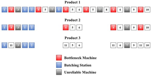
The simulation model is made up of 11 work centres, each with one server except the bottleneck work centre (work centre 4) that has two servers. The processing times for the work centres are log-normally distributed with the standard deviation less than or equal to 10 percent of the mean. Table 1 shows the specific work centre processing times and the respective batch sizes.

Table 1. Processing times and batch sizes.

Work centre #	Mean	Std. Dev.	Batch (Min/Max)
1	80	7	2/4
2	220	16	2/4
3	45	4	1
4	40	4	1
5	25	2	1
6	22	2.4	1
7	20	2	1
8	100	12	1
9	50	4	1
10	50	5	1
11	70	2.5	1

Machines 3 and 7 are subject to machine failures, whose time to failure (MTTF) and time to repair (MTTR) follow gamma distributions with the following parameters that are the same for both machines:

• MTTF: $\alpha =7200$, $\text{β}=1⟹\mathrm{M}\mathrm{e}\mathrm{a}\mathrm{n}=7200$, $\mathrm{S}\mathrm{t}\mathrm{d}.\mathrm{D}\mathrm{e}\mathrm{v}.=84.9$

• MTTR: $\alpha =1200$, $\text{β}=1.5⟹\mathrm{M}\mathrm{e}\mathrm{a}\mathrm{n}=1800$, $\mathrm{S}\mathrm{t}\mathrm{d}.\mathrm{D}\mathrm{e}\mathrm{v}.=52.0$

The low process variance is representative of automation and tight process specifications encountered in the semiconductor industry. A visit to a work centre is defined as a process step and will be referred to as a ‘step’ for consistency. Three products are produced in the system which have varying number of process steps, representing the differing complexity among products: Product 1 has 22 process steps including 6 visits to the bottleneck work centre, product 2 has 14 process steps with 4 visits to the bottleneck work centre and product 3 has 14 process steps and does not visit the bottleneck. The system is required to produce a product mix that is 3:1:1 of Product 1, 2, and 3 respectively.

In the simulation model, there are two work centres with low reliability that create most of the starvation at the bottleneck. One work centre is visited only once by each product early in the process routings; the physical location early in the process lends this step to act as a ‘gateway operation’ because of its ability to restrict the flow of the product into the system. The second work centre capable of starving the bottleneck is a re-entrant work centre that is visited multiple times by the products and occurs later in the routings. This work centre is representative of a Chemical Vapor Deposition (CVD) process that is capable of producing a high output very quickly. These two unreliable work centres have the ability to produce many products in a very short period of time but can starve the bottleneck due to poor availability. The demand is assumed to be stochastic with exponentially distributed inter–arrival times. Orders arrive with a mean of one order per 98 minutes and the due dates are set as follows (Kutanoglu 1999; Land 2006; Gupta and Sivakumar 2007; Bahaji and Kuhl 2008; Thuerer, Silva, and Stevenson 2011):

On arrival the product type is randomly assigned by a discrete uniform distribution dunif{1,5} (1-3: product type 1, 4: product type 2, and 5: product type 3 to represent the product mix) and the due date is determined by adding a random allowance where the minimum slack is defined as seven times the total processing time of product type 1 (7868 minutes) and the maximum slack is set to 14,612 minutes (13 times total processing time of product type 1). Thus (5) $D{D}_j=A{T}_j+unif\{7868;\mathrm{14,612}\}$(5) where $D{D}_j$ denotes the due date and $A{T}_j$ the arrival time of order j. The random allowance was set such that an Immediate Release strategy yields a percentage of tardy jobs between 0% and 5%. Although any individual semiconductor wafer fab in practice will differ in many aspects from our stylised environment, we think that our simulation model still captures the general characteristics of semiconductor manufacturing, such as: (i) reliability (hard failures in terms of machine breakdowns), (ii) re-entrant process flows and (iii) mixed processing modes (individual items vs. multi-lot batches) (see e.g. Fowler, Hogg, and Mason 2002). Having described the simulation model, we now discuss the experimental design which is depicted in Table 2.

Table 2. Experimental design.

Pool Sequencing Rule	Order Release Model	Tested Parameters
FCFS	Starvation Avoidance (SA)	α (2; 2.5; 3; 3.5; 4; 4.5;
		5; 5.5; 6; 6.5; 7)
	LUMS-COR	α (2; 3; 4)
		workload norm (100; 200; 300; 400;
		500; 600; 700; 800; 900; 1,000)
	ConLOAD	ConLOAD Limit (1.9; 1.95; 2.0;
		2.05; 2.1; 2.15; 2.2;
		2.25; 2.3; 2.35; 2.4)
EDD	Starvation Avoidance (SA)	α (2; 2.5; 3; 3.5; 4; 4.5;
		5; 5.5; 6; 6.5; 7)
	LUMS-COR	α (2; 3; 4)
		workload norm (100; 200; 300; 400;
		500; 600; 700; 800; 900; 1,000)
	ConLOAD	ConLOAD Limit (1.9; 1.95; 2.0;
		2.05; 2.1; 2.15; 2.2;
		2.25; 2.3; 2.35; 2.4)
CR	Starvation Avoidance (SA)	α (2; 2.5; 3; 3.5; 4; 4.5;
		5; 5.5; 6; 6.5; 7)
	LUMS-COR	α (2; 3; 4)
		workload norm (100; 200; 300; 400;
		500; 600; 700; 800; 900; 1,000)
	ConLOAD	ConLOAD Limit (1.9; 1.95; 2.0;
		2.05; 2.1; 2.15; 2.2;
		2.25; 2.3; 2.35; 2.4)

The three above described order release approaches, SA, LUMS-COR and ConLOAD, are analysed with different sets of parameters and in conjunction with each of the three above described pool sequencing rules (see Table 2). SA and LUMS-COR are analysed with eleven and three different α-values, respectively, and we test ten workload norms for the LUMS-COR model. All parameters were specified based on pilot simulation runs. Moreover, eleven ConLOAD limits are considered for ConLOAD, and since ConLOAD requires the estimation of the average shop floor time for each product type, the average shop floor times were estimated by pilot simulation runs using an immediate release scenario. Thus, in total 156 different scenarios are simulated. The dispatching rule is First-In First-Out throughout all investigated scenarios. Therefore, the results are solely dependent on the specific Pool Sequencing rule, the underlying Order Release approach and the respective parameterisation.

The period length was set to 1440 minutes (one day), each scenario was replicated 80 times, the warm-up phase was set to 800 periods and data was collected over 1,000 periods. A cost function was defined to evaluate the results which consists of the sum of $WIP\left(WI{P}_{n,t}\right)$ at each work centre n, finished goods holding $FGI\left(FG{I}_t\right)$ and backorder $\left(B{O}_t\right)$ costs over all periods t: (6) $\begin{array}{r}\mathrm{T}\mathrm{o}\mathrm{t}\mathrm{a}\mathrm{l}\mathrm{C}\mathrm{o}\mathrm{s}\mathrm{t}\mathrm{s}=\sum _{t=1}^T\sum _{n=1}^N\omega WI{P}_{n,t}+\sum _{t=1}^T(\pi FG{I}_t+\kappa B{O}_t)\end{array}$(6) We set the cost parameters ω, π and κ in the following relation: $2\frac{1}{3}\mathrm{\$}:1\mathrm{\$}:3\frac{1}{3}\mathrm{\$}$ which is taken from earlier WLC studies in semiconductor industry (Kacar, Irdem, and Uzsoy 2012; Kacar, Moench, and Uzsoy 2013; Albey and Uzsoy 2015; Ziarnetzky et al. 2015).

5. Results

In this section, the results for the different pool sequencing rules are discussed together with analyses of all investigated pool sequencing rules for the different order release approaches. For brevity we present only a selection of our full factorial design, but provide the results for all simulated scenarios under http://dx.doi.org/10.17632/jhrzc4wgf5.3.

As common in WLC literature, we focus on the timing and balancing performance of the tested order release mechanisms. Therefore, we use a cost based comparison where we compare the WIP, finished goods inventory, backorder and total costs (see Equation (6(6) $\begin{array}{r}\mathrm{T}\mathrm{o}\mathrm{t}\mathrm{a}\mathrm{l}\mathrm{C}\mathrm{o}\mathrm{s}\mathrm{t}\mathrm{s}=\sum _{t=1}^T\sum _{n=1}^N\omega WI{P}_{n,t}+\sum _{t=1}^T(\pi FG{I}_t+\kappa B{O}_t)\end{array}$(6) )). This allows us to identify (i) the best parameterisation of each order release mechanism and (ii) the overall best approach. Thereafter, we use timing and load balancing measures (in minutes) for a more detailed analysis: the former consists of the order pool time, service level (% tardy), mean tardiness and earliness and the latter is represented by the mean and standard deviation of shop floor time and bottleneck queue time.

5.1. FCFS pool sequencing

Figure 2(a) shows the cost measures over all replications for selected scenarios under FCFS pool sequencing. For brevity, we use a double for SA and ConLOAD, and a triple to denote each LUMS-COR scenario: The first component corresponds to the order release mechanism (SA, LUMS for LUMS-COR or ConLOAD), the second denotes the tested α value (for SA and LUMS-COR) or the ConLOAD limit, and in the third component the numbers between 600–1000 represent the analysed workload norms for the bottleneck work centre. Each bar indicates the total costs of a scenario which is divided into its three components of backorder, WIP and inventory costs shown in red, orange and grey respectively.

Figure 2. Cost comparison between the different order release models for the investigated pool sequencing rules. (a) FCFS pool sequencing, (b) EDD pool sequencing and (c) CR pool sequencing.

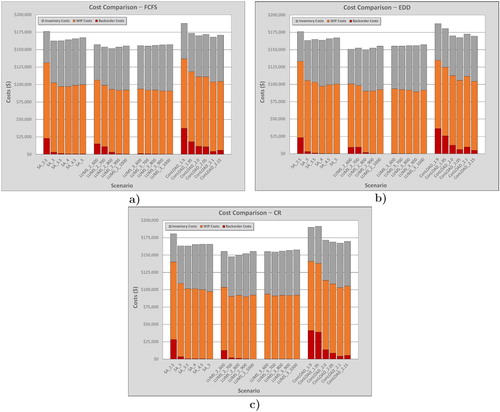
One can see in Figure 2(a) that, with regard to costs, all LUMS-COR scenarios yield lower total costs than the best performing parameterisation of the other release mechanisms (SA and ConLOAD). Furthermore one can see that the overall best scenario is LUMS_2_800 followed by LUMS_2_900. In comparison to the best performing LUMS-COR model, the best SA scenario (SA_3) yields $10,689.32 and the best ConLOAD scenario (ConLOAD_2.1) yields $16,352.51 higher average total costs. More precisely, LUMS_2_800 yields no significantly lower backorder costs but $9662.74 lower WIP costs and $5668.00 lower inventory costs than ConLOAD_2.1. Similarly, LUMS_2_800 yields $9203.85 lower WIP costs, but no significantly lower inventory costs and also no significantly lower backorder costs than SA_3 (also see Table A1 in the Appendix).

With regard to the parameterisation of the order release mechanisms we can conclude the following: Since high α values for the LUMS-COR and SA approach lead to earlier release of orders, backorder costs decrease and inventory costs increase with increasing α values. Additionally, for the SA approach one can also see an influence of the α value on its balancing performance (WIP costs): If the α value is too low the bottleneck is more likely to starve which increases the variability on the shop floor, while for high α values WIP costs increase due to more orders on the shop floor. The same relation holds for increasing workload norms (LUMS-COR) and the ConLOAD limit: the higher the norm or limit the lower backorder costs and thus higher are the inventory costs.

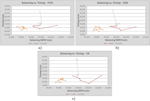
Figure 3(a) depicts the balancing and timing performance of each order release approach where the former is represented by WIP costs and the latter by the sum of inventory and backorder costs. Here the results of SA are depicted as a red line and each parameterisation is marked with a diamond, ConLOAD scenarios are represented by the grey line marked with triangles and the orange line with squares depicts the results for LUMS-COR. Figure 3(a) shows that LUMS-COR outperforms ConLOAD by yielding a better balancing and timing performance. In comparison to the SA method LUMS-COR yields similar timing, but also lower balancing (WIP) costs.

Figure 3. Comparison of balancing (WIP) and timing (inventory + backorder) costs for the different order release models for each investigated pool sequencing rule. (a) FCFS pool sequencing, (b) EDD pool sequencing and (c) CR pool sequencing.

The upper part of Table 3 shows detailed load balancing and timing measures for the three best performing parameterisations of the three order release mechanisms with FCFS pool sequencing. The first column denotes the tested order release approach and the corresponding parameterisation. Columns two, and seven to ten depict the timing measures, namely the order pool time, mean earliness, mean tardiness (all in minutes) and the proportions of orders which are late and early denoted as Tardy Jobs (%) and Early Jobs (%). Columns three to six depict the load balancing measures: the mean and standard deviation of shop floor time and the mean and standard deviation of bottleneck queue time (all in minutes). The shop floor time is the average time an order takes to traverse the system from order release to the end of production, whereas the bottleneck queue time is the average time an order is waiting at the bottleneck work centre prior to being processed. We compare each scenario with the best performing scenario with regard to average total costs (LUMS_2_800, see Figure 2(a)) at a significance level of p = 0.05 using a Wilcoxon/Mann-Whitney-U Test. The values marked with an asterisk are not significantly different from the best performing model which is highlighted in bold.

Table 3. Performance measures for the best order release scenarios for each investigated pool sequencing rule.

		Shop Floor Time		Bottleneck Queue Time
Scenario	Mean Order Pool Time	Mean	Std. Dev.	Mean	Std. Dev.	Mean Tardiness	Mean Earliness	Percentage Tardy Jobs	Percentage Early Jobs
FCFS pool sequencing
SA_3	1260.97*	4185.57*	1723.15	221.80	183.03	93.90*	5886.72*	5.19%*	94.81%*
LUMS_2_800	1280.97	4301.57	1535.27	297.53	209.96	88.81	5744.22	4.59%	95.41%
ConLOAD_2.1	860.68	4195.78	1584.80*	340.10	204.36*	116.82*	6299.97	4.07%*	95.93%*
EDD pool sequencing
SA_3	1381.64	4297.74*	1781.30	231.64	192.12	91.62	5653.78*	4.71%	95.29%
LUMS_2_800	1264.22	4235.15	1502.03	291.62	202.01	54.18	5793.69	2.77%	97.23%
ConLOAD_2.05	1176.80	4190.16*	1564.90	334.95	199.16*	177.08*	6049.63	5.47%*	94.53%*
CR pool sequencing
SA_3.5	968.34	4249.31*	1677.63	242.74*	191.08*	17.86*	6040.19	1.80%*	98.20%*
LUMS_2_700	1501.36	4186.62	1448.02	252.11	187.29	62.72	5615.11	3.10%	96.90%
ConLOAD_2.1	926.53	4161.63*	1555.07	335.95	205.14	123.24	6276.78	3.71%*	96.29%*

${}^{\ast }$Not significant (p<0.05).

In the following, we omit the parameterisation in the notation of the best performing scenarios (LUMS_2_800, SA_3, ConLOAD_2.1) and simply denote them as ‘LUMS-COR’, ‘SA’ or ‘ConLOAD’. One can see that, in comparison to SA, LUMS-COR yields slightly better (not significant) timing measures, namely slightly higher order pool time, lower mean tardiness and thus a slightly higher service level (% early). With regard to load balancing measures LUMS-COR, on the one hand, yields a slightly higher (not significant) shop floor time, but significantly lower standard deviation of shop floor time (187.88 minutes). On the other hand, LUMS-COR results in slightly, but significantly higher mean (75.74 minutes) and standard deviation (26.93 minutes) of bottleneck queue time. In comparison to ConLOAD, LUMS-COR releases orders later (420.29 minutes higher average order pool time) but does not yield significantly different tardiness measures (no significantly lower mean tardiness and no significantly higher percentage of tardy orders). Nevertheless, LUMS-COR yields a significantly lower mean earliness (555.76 minutes). Moreover regarding load balancing measures, LUMS-COR yields a slightly higher mean shop floor time (105.79 minutes) but a significantly lower mean bottleneck queue time (42.56 minutes) than ConLOAD.

The results for FCFS pool sequencing can be summarised as follows: (i) LUMS-COR yields the lowest total costs which is mainly due to the low WIP costs, which result from the lowest standard deviation of shop floor time (not significant compared to ConLOAD), (ii) all of the best performing parameterisations of the three order release strategies yield a service level (% early) close to 95% and (iii) SA performs best regarding bottleneck queue time.

5.2. EDD pool sequencing

Figure 2(b) shows the cost measures for selected scenarios under EDD pool sequencing. One can see that changing the pool sequencing rule from FCFS to EDD sequencing has little impact on the (relative) performance of the order release mechanisms: As above, the best scenario with regard to total costs is LUMS_2_800 followed by several other parameterisations of the LUMS-COR approach. Different from the results for FCFS pool sequencing, the influence of the workload norm on the WIP costs is more pronounced: For low workload norm levels the bottleneck is more likely to starve which increases the variability on the shop floor and, on the other, for high workload norms costs increase due to more orders on the shop floor. In comparison to LUMS-COR, the best SA scenario SA_3 yields $13,945.15 and the best ConLOAD scenario ConLOAD_2.05 yields $18,267.55 higher average total costs (also see Table A2 in the Appendix).

Similarly, there is no difference from FCFS pool sequencing in the relative performance of the three order release approaches when comparing the WIP and timing costs (see Figure 3(b)). LUMS-COR also outperforms ConLOAD and in comparison to SA yields lower WIP, but similar timing costs.

The middle part of Table 3 shows detailed timing and load balancing measures for the best performing scenarios for EDD pool sequencing. Again, the results are only slightly different from those for FCFS pool sequencing: The SA and ConLOAD order release mechanisms yield a service level (% early) close to 95% and LUMS-COR yields a service level above 97%. Moreover, LUMS-COR yields the lowest standard deviation of shop floor time and SA performs best regarding bottleneck queue time.

5.3. CR pool sequencing

Figure 2(c) shows the cost measures for selected scenarios under CR pool sequencing. Again, all depicted LUMS-COR scenarios yield lower costs than the best parameterisations of SA and ConLOAD. The lowest total cost value is obtained by the LUMS_2_700 scenario followed by LUMS_2_800 which has significant higher total costs. With CR pool sequencing the best performing LUMS-COR model outperforms the best SA (SA_3.5) and ConLOAD (ConLOAD_2.1) scenario by yielding lower WIP and inventory costs and lower or not significantly different backorder costs. In total SA yields $15,361.25 and ConLOAD $19,537.18 higher average total costs (also see Table A3 in the Appendix).

Similarly, there is no difference from the above results in terms of the WIP and timing costs (see Figure 3(c)). LUMS-COR also outperforms ConLOAD and yields lower WIP than SA, but similar timing costs. With regard to timing measures, depicted in the bottom part of Table 3, LUMS-COR outperforms the other order release mechanisms by yielding higher order pool time, lower or not significantly different tardiness and percentage of tardy orders, but significantly lower earliness. Concerning load balancing, LUMS-COR yields no significantly different shop floor time, but the lowest standard deviation thereof. Interestingly with CR pool sequencing, LUMS-COR can close the gap with regard to bottleneck queue time (both mean and standard deviation).

To sum up, we have shown that, independent of the pool sequencing rule, LUMS-COR yields the lowest total costs mainly due to its superior balancing performance. This is consistent with earlier research that compared LUMS-COR to other continuous order release mechanisms in balanced shops (Thuerer et al. 2012). The advantages of LUMS-COR are twofold: First, in contrast to the purely continuous methods (SA and ConLOAD), LUMS-COR uses both a periodic and a continuous element: the former levels the workload fluctuations while the latter avoids starvation of the bottleneck work centre. Second, the workload calculation of LUMS-COR is the most accurate, since it divides the contributed workload by the position of a work centre in the routing while SA and ConLOAD at best only partially differentiate between the workload contributions of the different bottleneck visits. The superior timing performance of LUMS-COR in comparison to ConLOAD can be explained by the difference of workload aggregations: Similar to ConWIP, ConLOAD updates the workload contribution after the order leaves the shop floor while LUMS-COR updates whenever a process step is finished.

5.4. Influence of pool sequencing rules on performance of each order release approach

When comparing the best performing parameterisation (based on cost measures) of each pool sequencing rule (see Table 3), the following can be concluded: While the shop floor times do not significantly differ for the best SA models, EDD and CR pool sequencing yield slightly but significantly lower percentages of tardy jobs (0.47% and 3.39%) compared to FCFS pool sequencing. With regard to load balancing measures, there are no significant differences between the best parameterisations for the standard deviation of shop floor time and the mean and standard deviation of bottleneck queue time, except for the mean bottleneck queue time under FCFS which is slightly but significantly lower (20.94 minutes) compared to CR. With regard to cost measures (see Tables A1 to A3 in the Appendix), we do not see an influence of pool sequencing rules on the SA method, since there is no significant difference between the best parameterisations in terms of total costs.

When focussing on the best ConLOAD and LUMS-COR models (based on cost measures; see Table 3) the following can be concluded: Only CR under LUMS-COR yields a significantly lower shop floor time (114.94 minutes) than under FCFS. Similarly, CR sequencing yields a lower or equal percentage of tardy orders in comparison to the other two sequencing rules. Nevertheless, EDD yields 1.81% fewer tardy orders under LUMS-COR but 1.40% more tardy orders under ConLOAD compared to FCFS, respectively. Moreover, with CR pool sequencing LUMS-COR order release yields a significantly higher order pool time, namely 237.14 minutes higher in comparison to EDD and 220.40 minutes higher than FCFS sequencing. Under ConLOAD, there are no significantly different order pool times.

While the load balancing performance under ConLOAD is quite similar for EDD and CR pool sequencing, both EDD and CR yield better load balancing performance compared to FCFS. LUMS-COR yields the best load balancing performance under CR pool sequencing: Here, not only the standard deviation of shop floor time, but also the mean bottleneck queue time and standard deviation thereof can be reduced: CR sequencing yields 94.32% and 96.40% of the standard deviation of the shop floor time, 84.73% and 86.45% in bottleneck queue time and 89.20% and 92.71% in standard deviation of bottleneck queue time all compared to FCFS and EDD respectively. Finally, both order release models (ConLOAD and LUMS-COR) yield the lowest total costs under CR pool sequencing (see Tables A1 to A3 in the Appendix)).

Overall, we conclude that for ConLOAD and LUMS-COR the CR pool sequencing rule should be used.

5.5. Sensitivity analysis

In this subsection, the different order release approaches are analysed in different settings. More precisely, different product mixes, failure rates, the release procedure for non-bottleneck products and the application of a workload norm under LUMS-COR for all work centres are investigated. For brevity we present the sensitivity analysis only for CR pool sequencing and limit our interpretation to cost measures. Note that the results of the sensitivity analysis for FCFS and EDD pool sequencing and all timing and balancing measures are available under http://dx.doi.org/10.17632/jhrzc4wgf5.3.

5.5.1. Different product mixes

Three different product mixes are investigated in the following. More precisely, the proportion of non-bottleneck products is reduced step-wise to 0: starting from the originally product mix of 3:1:1 (i.e. 60:20:20) to 65:25:10 and 70:30:0 which means that the lower proportion of non-bottleneck products is equally distributed over products 1 and 2. For both new product mixes, the demand was parameterised such that again the bottleneck utilisation equals approximately 90%. Note that the best performing scenario from each order release mechanism under the original product mix was used for the two altered product mixes. Table 4 shows the cost measures for the best SA, LUMS-COR and ConLOAD scenarios under CR pool sequencing. One can see that, reducing the proportion of non-bottleneck products has little impact on the relative performance of the order release mechanisms: LUMS-COR yields the lowest total costs, mainly due to significantly lower WIP and inventory costs compared to SA and ConLOAD.¹

Table 4. Cost measures for the best order release scenarios for different product mixes under CR pool sequencing.

Scenario	Backorder Costs	WIP Costs	Inventory Costs	Total Costs
Product Mix 60:20:20
SA_3.5	$606.35*	$100,933.12	$61,517.35	$163,056.83
LUMS_2_700	$2126.41	$88,351.15	$57,218.01	$147,695.58
ConLOAD_2.1	$4205.04	$98,983.00	$64,044.71	$167,232.76
Product Mix 65:25:10
SA_3.5	$429.70*	$89,628.02	$54,037.03	$144,094.74
LUMS_2_700	$3334.83	$80,019.31	$50,186.90	$133,541.04
ConLOAD_2.1	$6847.40*	$90,205.22	$56,504.21	$153,556.83
Product Mix 70:30:0
SA_3.5	$328.21*	$82,676.15	$47,766.48	$130,770.84
LUMS_2_700	$8529.25	$75,290.89	$41,889.86	$125,710.01
ConLOAD_2.1	$7062.47*	$87,169.96	$47,639.03	$141,871.46

${}^{\ast }$ Not significant (p<0.05).

5.5.2. Long failures

In the original setting, short failure times were applied. Therefore, in this subsection a long failure setting is applied which means that the machine failures of machines 3 and 7 or more precisely, their time to failure (MTTF) and time to repair (MTTR) are now characterised by gamma distributions with the following parameters that are the same for both machines:

• MTTF: $\alpha =\mathrm{14,400}$, $\text{β}=1⟹\mathrm{M}\mathrm{e}\mathrm{a}\mathrm{n}=\mathrm{14,400}$, $\mathrm{S}\mathrm{t}\mathrm{d}.\mathrm{D}\mathrm{e}\mathrm{v}.=120$

• MTTR: $\alpha =2400$, $\text{β}=1.5⟹\mathrm{M}\mathrm{e}\mathrm{a}\mathrm{n}=3600$, $\mathrm{S}\mathrm{t}\mathrm{d}.\mathrm{D}\mathrm{e}\mathrm{v}.=73.5$

Since the average availability does not change with these longer failure times, the demand remains the same as in the short failure setting. Nevertheless, pre-simulation runs were performed to determine suitable parameters for the single order release approaches. More precisely,

• for SA, the α-value was varied from 4 to 10 in steps of 1,

• for LUMS-COR, the workload norm was varied from 700 to 1100 and the α-value was set to 4, and

• for ConLOAD, the ConLOAD limit was varied from 2.45 to 2.75 in steps of 0.05.²

Table 5 shows the cost measures for the best scenarios for short and long failures under CR pool sequencing. As can be seen, LUMS-COR yields significantly lower total costs by yielding lower WIP and inventory costs compared to SA and ConLOAD. This means that under the long failure scenario the comparative advantage of LUMS-COR is sustained.

Table 5. Cost measures for the best order release scenarios for different failure times under CR pool sequencing.

Scenario	Backorder Costs	WIP Costs	Inventory Costs	Total Costs
Short failures
SA_3.5	$606.35*	$100,933.12	$61,517.35	$163,056.83
LUMS_2_700	$2126.41	$88,351.15	$57,218.01	$147,695.58
ConLOAD_2.1	$4205.04	$98,983.00	$64,044.71	$167,232.76
Long failures
SA_9	$8723.85*	$151,037.18	$44,555.16	$204,316.20
LUMS_4_1000	$8779.96	$138,733.27	$40,476.89	$187,990.12
ConLOAD_2.65	$11,151.63*	$158,138.64	$47,399.75	$216,690.02

${}^{\ast }$ Not significant (p<0.05).

5.5.3. Including a time limit for non-bottleneck products

In the original setting, all investigated order release approaches were either designed (SA and ConLOAD) or adapted (LUMS-COR) to control only bottleneck products and therefore, non-bottleneck products are either immediately released (SA and ConLOAD) or released at the beginning of the following period (LUMS-COR). However, in this subsection a time limit is applied to non-bottleneck products which means that under SA and ConLOAD, arriving non-bottleneck products are released whenever their due date is within the time limit. Regarding LUMS-COR, non-bottleneck products are still released at periodic intervals but only if their due date is within the time limit. The best parameterisation of each order release mechanism under the original setting is used. Nevertheless, eight different time limits (2880 through 12,960 in steps of 1440) for non-bottleneck products were tested and the best time limit for each release approach in terms of total costs is presented in the following.³

Table 6 shows the cost measures for the best scenarios without and with a time limit for non-bottleneck products under CR pool sequencing. Note that in the lower part of Table 6, i.e. the scenarios with a time limit, an additional component in the notation is used to indicate the time limit. LUMS-COR yields significantly lower total costs than SA and ConLOAD in both scenarios: With uncontrolled release of non-bottleneck products (upper part of Table 6), LUMS-COR yields similar or lower backorder costs and lower WIP and inventory costs than SA and ConLOAD. However, with controlled release of non-bottleneck products (lower part of Table 6), LUMS-COR yields slightly higher backorder costs which are outweighed by a significant WIP and inventory cost reduction. Generally, including a time limit for non-bottleneck products improves the cost performance for all order release approaches, but the LUMS-COR approach utilises the limited time limit best, since it can also improve the balancing performance (WIP costs).

Table 6. Cost measures for the best order release scenarios under CR pool sequencing without and with a time limit for non-bottleneck products.

Scenario	Backorder Costs	WIP Costs	Inventory Costs	Total Costs
Without time limit for non-bottleneck products
SA_3.5	$606.35*	$100,933.12	$61,517.35	$163,056.83
LUMS_2_700	$2126.41	$88,351.15	$57,218.01	$147,695.58
ConLOAD_2.1	$4205.04	$98,983.00	$64,044.71	$167,232.76
With time limit for non-bottleneck products
SA_3.5_4320	$1525.64	$100,334.37	$47,182.14	$149,042.15
LUMS_2_700_4320	$4756.57	$85,785.71	$42,759.98	$133,302.25
ConLOAD_2.1_4320	$4012.86	$99,924.44	$48,309.36	$152,246.66

${}^{\ast }$ Not significant (p<0.05).

5.5.4. LUMS-COR all work centres

In this subsection, the potential of applying a workload norm not only to the bottleneck work centre but rather to all work centres is investigated. Therefore, non-bottleneck products are not released at periodic intervals without considering their workload contribution, but only if they do not violate the workload norms of the work centres in their routing. Multiple scenarios (alpha-values 2 and 3 and workload norms from 800 to 1700 in steps of 100) have been simulated but only the best (in terms of costs) scenarios for each alpha-value ± two surrounding parameterisations are presented in the following⁴ and are compared to the overall best performing bottleneck LUMS-COR scenario (i.e. LUMS_BN_2_700) at a significance level of p = 0.05 using a Wilcoxon/Mann-Whitney-U Test. Regarding the notation it is to be mentioned that a quadruple was used: the first component denotes the LUMS-COR order release approach, the second component describes whether a workload norm is applied to only the bottleneck (i.e. BN) or all work centres (i.e. allWCs), the third component denotes the α-value and the fourth component represents the workload norm.

Table 7 shows the cost measures for different parameterisations for LUMS-COR order release with a workload norm applied only to the bottleneck and all work centres under CR pool sequencing. One can see that, compared to LUMS_BN_2_700, LUMS_allWCs_2_1500 leads to slightly lower total costs on average. More precisely, LUMS_allWCs_2_1500 yields significantly higher backorder costs but significantly lower inventory costs and no significantly higher WIP costs.

Table 7. Cost measures for different parameterisations for LUMS-COR order release with a workload norm for only the bottleneck and all work centres under CR pool sequencing.

Scenario	Backorder costs	WIP costs	Inventory costs	Total costs
LUMS_BN_2_700	$2126.41	$88,351.15	$57,218.01	$147,695.58
LUMS_allWCs_2_1300	$31,301.96	$96,883.00	$35,523.00	$163,707.96*
LUMS_allWCs_2_1400	$18,326.24	$89,231.63*	$42,928.60	$150,486.47
LUMS_allWCs_2_1500	$9679.60	$89,924.54*	$46,194.36	$145,798.51
LUMS_allWCs_2_1600	$6975.14	$89,208.16*	$49,843.73	$146,027.02
LUMS_allWCs_2_1700	$4100.44*	$90,798.41*	$51,839.15	$146,738.00*
LUMS_allWCs_3_1000	$3646.64	$96,893.37	$49,586.79	$150,126.80
LUMS_allWCs_3_1100	$2487.26	$98,173.12	$50,777.41	$151,437.80
LUMS_allWCs_3_1200	$961.54*	$92,859.99	$55,818.24*	$149,639.77
LUMS_allWCs_3_1300	$586.79*	$92,504.52	$57,368.33*	$150,459.64
LUMS_allWCs_3_1400	$176.82	$89,451.61*	$60,952.89	$150,581.32

${}^{\ast }$ Not significant (p<0.05).

Concluding, we show that the proposed LUMS-COR approach that only applies a workload norm to the bottleneck work centre (LUMS_BN) performs quite well in terms of costs. One reason why the bottleneck-oriented LUMS-COR approach performs quite well is that non-bottleneck products have a low share in the total number of orders in the system (20%) and thus they do not seriously impact the systems' performance by large numbers. While LUMS_BN only controls bottleneck products (non-bottleneck products are released at periodic intervals), the original LUMS-COR approach controls all products by directing the load contributions of a job to workload norms for each work centre. Therefore, non-bottleneck products are only released if they fit within these norms. While the balancing performance (WIP costs) is not significantly different, LUMS_allWCs introduces more tardy orders (higher backorder costs) due to delaying non-bottleneck products, but reduces inventory costs as non-bottleneck products are also controlled and are not released too far ahead of their due date.

All in all, the results of the sensitivity analysis demonstrate the robustness of our results: The comparative advantage of LUMS-COR over all other tested order release methods remains unchanged for different product mixes, machine failure distribution and when a time limit is used for the release of the non-bottleneck products. Finally, we show that the proposed LUMS-COR approach that only applies a workload norm to the bottleneck work centre (LUMS_BN) performs quite well compared to applying a workload norm to all work centres. Thus, this study highlights the applicability of a rule based order release model – the LUMS-COR mechanism – to semiconductor industry.

6. Conclusion

This paper compared three rule based order release models based on workload control (WLC), the LUMS-COR (Thuerer et al. 2012), ConLOAD (Rose 1999) and Starvation Avoidance (SA) model (Glassey and Resende 1988), which are considered to be the best performing rule based order release approaches from largely separately developed streams of research: LUMS-COR is widely used in Small and Medium Enterprises in Make-To-Order environments (Oosterman, Land, and Gaalman 2000; Thuerer et al. 2012) and the latter two are mostly used in semiconductor manufacturing (Glassey and Resende 1988; Cogez 1990; Glassey 1990; Framinan, González, and Ruiz-Usano 2003). One of the main differences between these approaches is that SA and ConLOAD are purely continuous and LUMS-COR is a hybrid approach, meaning that it includes periodic and continuous elements to make the order release decision. Since recent research on semiconductor manufacturing has not taken advantage of some of the latest developments in the rule based WLC literature, i.e. the LUMS-COR method introduced in Thuerer et al. (2012), this paper takes a first step and analyses whether an adapted LUMS-COR approach improves the performance of rule based WLC approaches in semiconductor wafer fabs. Furthermore, research on semiconductor wafer fabs has neglected pool sequencing rules, although several WLC studies highlighted their important influence on performance within rule based order release models (Thuerer et al. 2015, 2017a). Thus, we also analyse whether pool sequencing rules impact the performance of rule based order release models in semiconductor manufacturing. Therefore, we use a simulation model of a scaled-down wafer fabrication facility (Kayton et al. 1997) and evaluate the performance of all three order release approaches by using cost, timing and load balancing measures.

With regard to cost measures, we find that our adapted LUMS-COR yields the lowest total costs for all pool sequencing rules. This is mainly due to the superiority of LUMS-COR regarding load balancing, yielding the lowest standard deviation of shop floor time over all scenarios without worsening the tardiness. The only load balancing measure where LUMS-COR is outperformed is, as expected, the bottleneck queue time where the SA approach remains the best performer. However, these findings show that the LUMS-COR approach is a viable alternative for order release in semiconductor manufacturing. Moreover, our sensitivity analysis showed that the performance of the adapted LUMS-COR approach is also robust across different settings (i.e. product mixes, failure times, treatment of non-bottleneck products and application of workload norm to bottleneck or all work centres). Focusing on our analysis of the influence of pool sequencing rules on the performance of order release models in semiconductor wafer fabs our conclusions are twofold: (i) there is hardly any influence of pool sequencing on the performance of the SA approach and (ii) for ConLOAD and LUMS-COR, CR pool sequencing outperforms the other tested rules, especially with regard to balancing under LUMS-COR and timing under ConLOAD and thus are recommended for these two order release models. With regard to using LUMS-COR in practice, especially the periodical element of LUMS-COR should ease the implementation, since it was often argued that periodic decision making is thought to be a better fit with the behaviour of planners who typically make release decisions once a shift or day (Hendry and Kingsman 1991; Sabuncuoglu and Karapınar 1999; Stevenson et al. 2011; Thuerer et al. 2012). Furthermore, in comparison to earlier purely periodic WLC methods, the LUMS-COR model has the advantage of setting only one initial WLC norm.

The study provides important insights, but we are aware of its limitations. Firstly, the results are limited to the simulated case and the validity of the results for e.g. large-scale semiconductor fabs must be assessed in future studies. Secondly, adding further experimental factors would be beneficial like analysing different demand patterns or including different scheduling rules. Furthermore, future studies should also compare the LUMS-COR model to the widely used periodic optimisation based order release models in the semiconductor industry (Kacar, Irdem, and Uzsoy 2012; Kacar, Moench, and Uzsoy 2013; Ziarnetzky et al. 2015). Finally, another important future research direction is to address the problem of setting workload norms in large, complex fabs, and to demonstrate the applicability of LUMS-COR in high-mix environments representative of today's growing number of foundry fabs.

Acknowledgements

The authors would like to thank Reha Uzsoy, Hubert Missbauer, Matthias Thuerer, Quirin Ilmer, Manuel Schneckenreither and also four anonymous reviewers for their helpful comments and suggestions that greatly helped us to improve the paper.

Disclosure statement

No potential conflict of interest was reported by the author(s).

Additional information

Notes on contributors

Philipp Neuner

Philipp Neuner is currently working as research assistant at the Department of Information Systems, Production and Logistics Management at the University of Innsbruck. He received his M.Sc. degree in Information Systems from the University of Innsbruck in 2019 and is currently studying for his PhD degree in Management at the University of Innsbruck.

Stefan Haeussler

Stefan Haeussler is currently Assistant Professor at the Department of Information Systems, Production and Logistics Management at the University of Innsbruck. He received his PhD from the University of Innsbruck, School of Management. His areas of interest include manufacturing planning and control, simulation modeling, workload control, optimization models, forecasting, regression and behavioral operations management.

Notes

1 Note that due to different parameterised inter-arrival times to achieve the desired 90% bottleneck utilisation, the results of the different product mixes are not directly comparable.

2 Note that the results for all simulated scenarios under the long failure setting are available under http://dx.doi.org/10.17632/jhrzc4wgf5.3.

3 Note that the results for all tested time limits are available under http://dx.doi.org/10.17632/jhrzc4wgf5.3.

4 Note that the results for all tested workload norms are available under http://dx.doi.org/10.17632/jhrzc4wgf5.3.

Appendix. Additional tables

Table A1 shows the cost measures over all replications for selected scenarios under FCFS pool sequencing. The first column denotes the tested order release approach and the corresponding parameterisation. For brevity, we use a double for SA and ConLOAD, and a triple to denote each LUMS-COR scenario (adapted to control the bottleneck workload): The first component corresponds to the order release mechanism (SA, LUMS for LUMS-COR or ConLOAD), the second component denotes the tested α value (for SA and LUMS-COR) or the ConLOAD limit, and in the third component the numbers between 600–1000 represent the analysed workload norms for the bottleneck work centre. The remaining columns depict the average Backorder, WIP, Inventory and Total Cost values over all replications which are compared to the best performing scenario at a significance level of p = 0.05 using a Wilcoxon/Mann-Whitney-U Test. The values marked with an asterisk are not significantly different from the best performing model which is highlighted in bold. Furthermore, to preserve readability we indicated the best performing scenario from each order release model in italics.

Table A1. Cost measures for different order release scenarios together with FCFS pool sequencing.

Scenario	Backorder Costs	WIP Costs	Inventory Costs	Total Costs
SA_2.5	$23,051.84	$108,165.74	$45,022.50	$176,240.08
SA_3	$3188.27${}^{\ast }$	$99,319.95	$59,933.61${}^{\ast }$	$162,441.83
SA_3.5	$1245.42	$95,926.57	$65,498.05	$162,670.04
SA_4	$699.67	$96,466.37	$67,009.85	$164,175.89
SA_4.5	$614.97	$98,185.56	$66,919.00	$165,719.53
SA_5	$657.80	$99,271.57	$67,316.84	$167,246.21
LUMS_2_600	$14,928.27	$91,332.42${}^{\ast }$	$50,813.19	$157,073.87${}^{\ast }$
LUMS_2_700	$11,077.12	$87,685.73${}^{\ast }$	$55,144.31	$153,907.17
LUMS_2_800	$3059.06	$90,116.10	$58,577.35	$151,752.51
LUMS_2_900	$929.36	$90,874.31${}^{\ast }$	$61,864.40	$153,668.07
LUMS_2_1000	$517.52	$91,645.45${}^{\ast }$	$63,259.23	$155,422.20
LUMS_3_600	$1013.86	$92,836.17${}^{\ast }$	$62,124.06	$155,974.09
LUMS_3_700	$842.45	$91,113.11${}^{\ast }$	$63,256.66	$155,212.22
LUMS_3_800	$742.42	$91,463.74${}^{\ast }$	$63,882.95	$156,089.12
LUMS_3_900	$296.95	$90,671.45${}^{\ast }$	$65,708.21	$156,676.62
LUMS_3_1000	$277.93	$90,675.12${}^{\ast }$	$66,298.28	$157,251.33
ConLOAD_1.9	$37,299.12	$99,432.37	$50,967.94	$187,699.43
ConLOAD_1.95	$18,024.33	$100,285.18	$55,178.24${}^{\ast }$	$173,487.75
ConLOAD_2.0	$11,515.35	$99,568.01	$58,869.64${}^{\ast }$	$169,952.99
ConLOAD_2.05	$10,983.76${}^{\ast }$	$100,248.92	$60,661.24	$171,893.91
ConLOAD_2.1	$4080.83${}^{\ast }$	$99,778.84	$64,245.35	$168,105.02
ConLOAD_2.15	$6,050.24${}^{\ast }$	$98,616.90	$65,985.50	$170,652.64

${}^{\ast }$ Not significant (p<0.05).

Table A2 shows the cost measures for selected scenarios under EDD pool sequencing.

Table A2. Cost measures for different order release scenarios together with EDD pool sequencing.

Scenario	Backorder Costs	WIP Costs	Inventory Costs	Total Costs
SA_2.5	$23,218.01	$110,011.62	$42,887.75	$176,117.38
SA_3	$3140.52	$102,310.47	$57,706.59${}^{\ast }$	$163,157.59
SA_3.5	$1074.55	$101,816.54	$61,919.96${}^{\ast }$	$164,811.06
SA_4	$504.12${}^{\ast }$	$96,918.36	$66,305.75	$163,728.23
SA_4.5	$270.90${}^{\ast }$	$99,061.73	$66,585.06	$165,917.68
SA_5	$213.29${}^{\ast }$	$100,242.95	$66,782.03	$167,238.26
LUMS_2_600	$9247.62	$91,325.31${}^{\ast }$	$50,349.26	$150,922.19${}^{\ast }$
LUMS_2_700	$9484.46	$88,934.56${}^{\ast }$	$54,130.70	$152,549.72${}^{\ast }$
LUMS_2_800	$1882.03	$88,352.93	$58,977.48	$149,212.44
LUMS_2_900	$378.33${}^{\ast }$	$90,141.00${}^{\ast }$	$61,942.71${}^{\ast }$	$152,462.04
LUMS_2_1000	$89.83${}^{\ast }$	$92,244.85	$62,921.76	$155,256.43
LUMS_3_600	$393.23${}^{\ast }$	$93,192.37	$61,654.05${}^{\ast }$	$155,239.65
LUMS_3_700	$167.00${}^{\ast }$	$92,179.84	$62,843.21	$155,190.05
LUMS_3_800	$193.47	$91,480.58	$64,088.18	$155,762.22
LUMS_3_900	$45.12	$89,472.64${}^{\ast }$	$66,422.64	$155,940.40
LUMS_3_1000	$76.01${}^{\ast }$	$91,479.79	$65,704.35	$157,260.15
ConLOAD_1.9	$36,476.03	$98,160.98	$52,985.44${}^{\ast }$	$187,622.44
ConLOAD_1.95	$25,742.15	$98,949.01	$55,588.53${}^{\ast }$	$180,279.69
ConLOAD_2.0	$12,434.76	$100,159.19	$57,436.83${}^{\ast }$	$170,030.77
ConLOAD_2.05	$6065.80${}^{\ast }$	$99,680.31	$61,733.88	$167,479.99
ConLOAD_2.1	$9614.96	$101,870.69	$60,947.16${}^{\ast }$	$172,432.81
ConLOAD_2.15	$4858.18	$99,433.36	$65,346.18	$169,637.72

${}^{\ast }$ Not significant (p<0.05).

Table A3 shows the cost measures over all replications for selected scenarios under CR pool sequencing.

Table A3. Cost Measures for different order release scenarios together with CR pool sequencing.

Scenario	Backorder Costs	WIP Costs	Inventory Costs	Total Costs
SA_2.5	$28,297.34	$111,754.31	$40,683.30	$180,734.96
SA_3	$3528.05	$105,334.93	$54,289.44	$163,152.42
SA_3.5	$606.35${}^{\ast }$	$100,933.12	$61,517.35	$163,056.83
SA_4	$692.81${}^{\ast }$	$100,659.44	$63,806.14	$165,158.38
SA_4.5	$326.71${}^{\ast }$	$99,722.34	$65,511.60	$165,560.65
SA_5	$192.18	$97,196.04	$68,085.04	$165,473.26
LUMS_2_600	$12,562.88	$91,087.33${}^{\ast }$	$51,490.95	$155,141.16${}^{\ast }$
LUMS_2_700	$2,126.41	$88,351.15	$57,218.01	$147,695.58
LUMS_2_800	$1231.81${}^{\ast }$	$90,869.16${}^{\ast }$	$57,876.66${}^{\ast }$	$149,977.63
LUMS_2_900	$453.96	$89,700.31${}^{\ast }$	$61,988.24	$152,142.51
LUMS_2_1000	$91.99	$92,224.92	$62,908.94	$155,225.85
LUMS_3_600	$222.15	$93,348.68	$61,410.05	$154,980.89
LUMS_3_700	$163.17	$90,859.98${}^{\ast }$	$63,409.66	$154,432.81
LUMS_3_800	$107.31	$91,857.57	$63,681.00	$155,645.88
LUMS_3_900	$116.76	$91,771.51	$64,726.93	$156,615.19
LUMS_3_1000	$68.22	$92,222.45	$65,260.29	$157,550.96
ConLOAD_1.9	$41,147.94	$99,838.14	$49,012.10	$189,998.18
ConLOAD_1.95	$38,939.69	$98,975.25	$53,626.80${}^{\ast }$	$191,541.74
ConLOAD_2.0	$13,482.01${}^{\ast }$	$99,985.89	$57,969.55${}^{\ast }$	$171,437.45
ConLOAD_2.05	$8707.66${}^{\ast }$	$99,555.05	$60,576.21	$168,838.92
ConLOAD_2.1	$4205.04	$98,983.00	$64,044.71	$167,232.76
ConLOAD_2.15	$5440.60	$99,785.10	$64,580.31	$169,806.01

${}^{\ast }$ Not significant (p<0.05).

References

- Albey, E., and R. Uzsoy. 2015. “Lead Time Modeling in Production Planning.” In Proceedings of the 2015 Winter Simulation Conference, edited by L. Yilmaz, W. K. V. Chan, I. Moon, T. M. K. Roeder, C. Macal, and M. D. Rossetti, Piscataway, New Jersey, 1996–2007. Institute of Electrical and Electronics Engineers, Inc.
- Asmundsson, Jakob, Ronald L. Rardin, and Reha Uzsoy. 2006. “Tractable Nonlinear Production Planning Models for Semiconductor Wafer Fabrication Facilities.” IEEE Transactions on Semiconductor Manufacturing 19 (1): 95–111.
- Bahaji, N., and M. E. Kuhl. 2008. “A Simulation Study of New Multi-Objective Composite Dispatching Rules, CONWIP, and Push Lot Release in Semiconductor Fabrication.” International Journal of Production Research 46 (14): 3801–3824. https://doi.org/10.1080/00207540600711879.
- Bechte, Wolfgang. 1988. “Theory and Practice of Load-Oriented Manufacturing Control.” The International Journal of Production Research 26 (3): 375–395.
- Bechte, Wolfgang. 1994. “Load-Oriented Manufacturing Control Just-in-Time Production for Job Shops.” Production Planning & Control 5 (3): 292–307.
- Bergamaschi, D., R. Cigolini, M. Perona, and A. Portioli. 1997. “Order Review and Release Strategies in a Job Shop Environment: A Review and a Classification.” International Journal of Production Research 35 (2): 399–420.
- Bertrand, Jan Willem Marie, and Johan C. Wortmann. 1981. Production Control and Information Systems for Component Manufacturing Shops. New York: Elsevier Science Inc.
- Chen, Yarong, Hongming Zhou, Peiyu Huang, FuhDer Chou, and Shenquan Huang. 2019. “A Refined Order Release Method for Achieving Robustness of Non-Repetitive Dynamic Manufacturing System Performance.” Annals of Operations Research 1–15. https://doi.org/10.1007/s10479-019-03484-9.
- Cogez, P. 1990. The Effect of Uncertainty on Production Release Policies. Technical Report 90-25. U.C.Berkeley.
- de Kok, Ton G., and Jan C. CFransoo. 2003. “Planning Supply Chain Operations: Definition and Comparison of Planning Concepts.” Handbooks in Operations Research and Management Science 11: 597–675.
- Enns, S. T. 1995. “An Integrated System for Controlling Shop Loading and Work Flow.” International Journal of Production Research 33 (10): 2801–2820.
- Enns, S. T., and Myriam Prongué Costa. 2002. “The Effectiveness of Input Control Based on Aggregate Versus Bottleneck Work Loads.” Production Planning & Control 13 (7): 614–624.
- Fernandes, Nuno O., Martin J. Land, and Sílvio Carmo-Silva. 2014. “Workload Control in Unbalanced Job Shops.” International Journal of Production Research 52 (3): 679–690. https://doi.org/10.1080/00207543.2013.827808.
- Fowler, J. W., G. L. Hogg, and S. J. Mason. 2002. “Workload Control in the Semiconductor Industry.” Production Planning and Control 13 (7): 568–578.
- Framinan, Jose M., Pedro L. González, and Rafael Ruiz-Usano. 2003. “The CONWIP Production Control System: Review and Research Issues.” Production Planning & Control 14 (3): 255–265. https://doi.org/10.1080/0953728031000102595.
- Fredendall, Lawrence D., Divesh Ojha, and J. Wayne Patterson. 2010. “Concerning the Theory of Workload Control.” European Journal of Operational Research 201 (1): 99–111. <Go to ISI>: ://WOS:000272262100010.
- Glassey, P. G. 1990. Comparison of Release Rules using Blocs/M Simulations. Technical Report 90-15. U.C.Berkeley.
- Glassey, C. R., and M. G. C. Resende. 1988. “Closed-Loop Job Release Control for VLSI Circuit Manufacturing.” IEEE Transactions on Semiconductor Manufacturing 1 (1): 36–46.
- Glassey, C. R., J. G. Shanthikumar, and S. Seshadri. 1996. “Linear Control Rules for Production Control of Semiconductor Fabs.” IEEE Transactions on Semiconductor Manufacturing 9 (4): 536–549.
- Goldratt, E. M., and J. I. Cox. 1986. The Goal: A Process of Ongoing Improvement. New York: North River Press.
- Goldratt, E. M., and R. Fox. 1986. The Race. New York: North River Press.
- Gopalswamy, Karthick, and Reha Uzsoy. 2018. “An Exploratory Comparison of Clearing Function and Data-Driven Production Planning Models.” In 2018 Winter Simulation Conference (WSC), 3482–3493. IEEE.
- Gupta, Amit Kumar, and Appa Iyer Sivakumar. 2007. “Controlling Delivery Performance in Semiconductor Manufacturing Using Look Ahead Batching.” International Journal of Production Research 45 (3): 591–613. https://doi.org/10.1080/00207540600792226.
- Haeussler, S., and P. Netzer. 2019. “Comparison Between Rule- and Optimization Based Workload Control Concepts: A Simulation Optimization Approach.” International Journal of Production Research. Forthcoming.
- Haeussler, S., C. Stampfer, and H. Missbauer. 2020. “Comparison of Two Optimization Based Order Release Models with Fixed and Variable Lead Times.” International Journal of Production Economics227: 107682.
- Hendry, Linda. 1989. “A decision support system to manage delivery and manufacturing lead times in make-to-order companies.” Thesis, University of Lancaster.
- Hendry, Linda, and Brian Kingsman. 1991. “A Decision Support System for Job Release in Make-to-order Companies.” International Journal of Operations & Production Management 11 (6): 6–16.
- Hendry, L. C., and S. K. Wong. 1994. “Alternative Order Release Mechanisms: a Comparison by Simulation.” International Journal of Production Research 32 (12): 2827–2842. https://doi.org/10.1080/00207549408957103.
- Kacar, N. B., D. F. Irdem, and R. Uzsoy. 2012. “An Experimental Comparison of Production Planning Using Clearing Functions and Iterative Linear Programming-Simulation Algorithms.” IEEE Transactions on Semiconductor Manufacturing 25 (1): 104–117.
- Kacar, N. B., L. Moench, and R. Uzsoy. 2013. “Planning Wafer Starts Using Nonlinear Clearing Functions: A Large-Scale Experiment.” IEEE Transactions on Semiconductor Manufacturing 26 (4): 602–612.
- Kayton, D., T. Teyner, C. Schwartz, and R. Uzsoy. 1997. “Focusing Maintenance Improvement Efforts in a Wafer Fabrication Facility Operating Under the Theory of Constraints.” Production and Inventory Management Journal: Journal of the American Production and Inventory Control Society 38 (4): 51–57.
- Kingsman, B. G., I. P. Tatsiopoulos, and L. C. Hendry. 1989. “A Structural Methodology for Managing Manufacturing Lead Times in Make-to-Order Companies.” European Journal of Operational Research40 (2): 196–209. http://www.sciencedirect.com/science/article/pii/037722178990 3305.
- Kutanoglu, E. 1999. “An Analysis of Heuristics in a Dynamic Job Shop with Weighted Tardiness Objectives.” International Journal of Production Research 37 (1): 165–187. https://doi.org/10.1080/002075499191995.
- Land, Martin Jaap. 2004. “Workload control in job shops, grasping the tap.” Thesis, University Groningen.
- Land, Martin. 2006. “Parameters and Sensitivity in Workload Control.” International Journal of Production Economics 104 (2): 625–638. http://www.sciencedirect.com/science/article/pii/S09255273050 00617.
- Land, Martin, Mark Stevenson, and Matthias Thuerer. 2014. “Integrating Load-based Order Release and Priority Dispatching.” International Journal of Production Research 52 (4): 1059–1073. https://doi.org/10.1080/00207543.2013.836614.
- Lin, Yu-Hsin, and Ching-En Lee. 2001. “A Total Standard WIP Estimation Method for Wafer Fabrication.” European Journal of Operational Research 131 (1): 78–94. http://www.sciencedirect.com/science/article/pii/S03772217990 04464.
- Lou, S. X. C., and P. W. Kager. 1989. “A Robust Production Control Policy for VLSI Wafer Fabrication.” IEEE Transactions on Semiconductor Manufacturing 2 (4): 159–164.
- Lu, S. C. H., D. Ramaswamy, and P. R. Kumar. 1994. “Efficient Scheduling Policies to Reduce Mean and Variance of Cycle-time in Semiconductor Manufacturing Plants.” IEEE Transactions on Semiconductor Manufacturing 7 (3): 374–388.
- Melnyk, S. A., and G. L. Ragatz. 1989. “Order Review Release – Research Issues and Perspectives.” International Journal of Production Research 27 (7): 1081–1096.
- Missbauer, Hubert, and Reha Uzsoy. 2011. Optimization Models of Production Planning Problems, 437–507. Norwell: Springer.
- Mönch, Lars, J. W. Fowler, and Scott Mason. 2013. Production Planning and Control for Semiconductor Wafer Fabrication Facilities: Modeling, Analysis, and Systems. Heidelberg: Springer Science & Business Media.
- Mosley, S. A., T. Teyner, and R. M. Uzsoy. 1998. “Maintenance Scheduling and Staffing Policies in a Wafer Fabrication Facility.” IEEE Transactions on Semiconductor Manufacturing 11 (2): 316–323.
- Oosterman, Bas, Martin Land, and Gerard Gaalman. 2000. “The Influence of Shop Characteristics on Workload Control.” International Journal of Production Economics 68 (1): 107–119. http://www.sciencedirect.com/science/article/pii/S09255273990 01413.
- Puergstaller, Peter, and Hubert Missbauer. 2012. “Rule-based Vs. Optimisation-based Order Release in Workload Control: A Simulation Study of a MTO Manufacturer.” International Journal of Production Economics 140 (2): 670–680.
- Qi, C., A. I. Sivakumar, and S. B. Gershwin. 2007, December. “Simulation Experimental Investigation on Job Release Control in Semiconductor Wafer Fabrication.” In 2007 Winter Simulation Conference, Washington, DC, 1737–1746.
- Ragatz, G. J., and V. A. Mabert. 1988. “An Evaluation of Order Release Mechanisms in a Job-shop Environment.” Decision Sciences 19: 167–189.
- Resende, M. G. D. C. 1987. “Shop-Floor Scheduling of Semiconductor-Wafer Manufacturing.” Ph.D. diss., Department of Industrial Engineering and Operations Research, University of California, Berkeley, CA.
- Rose, O. 1999. “CONLOAD-A New Lot Release Rule for Semiconductor Wafer Fabs.” In WSC'99. 1999 Winter Simulation Conference Proceedings. ‘Simulation – A Bridge to the Future’ (Cat. No.99CH37038), Vol. 1, Phoenix, AZ, Dec., 850–855.
- Sabuncuoglu, I., and H. Y. Karapınar. 1999. “Analysis of Order Review/release Problems in Production Systems.” International Journal of Production Economics 62 (3): 259–279. http://www.sciencedirect.com/science/article/pii/S09255273980 02485.
- Spearman, Mark L., David L. Woodruff, and Wallace J. Hopp. 1990. “CONWIP: a Pull Alternative to Kanban.” International Journal of Production Research 28 (5): 879–894. http://www.tandfonline.com/doi/abs/10.1080/00207549008942761.
- Stevenson, Mark, Yuan Huang, Linda C. Hendry, and Erik Soepenberg. 2011. “The Theory and Practice of Workload Control: A Research Agenda and Implementation Strategy.” International Journal of Production Economics 131 (2): 689–700. http://www.sciencedirect.com/science/article/pii/S09255273110 00764.
- Sugimori, Y., K. Kusunoki, F. Cho, and S. Uchikawa. 1977. “Toyota Production System and Kanban System Materialization of Just-in-Time and Respect-for-Human System.” International Journal of Production Research 15 (6): 553–564. https://doi.org/10.1080/00207547708943149.
- Thuerer, Matthias, Nuno O. Fernandes, Mark Stevenson, and Ting Qu. 2017a. “On the Backlog-Sequencing Decision for Extending the Applicability of ConWIP to High-Variety Contexts: An Assessment by Simulation.” International Journal of Production Research 55 (16): 4695–4711. https://doi.org/10.1080/00207543.2017.1281462.
- Thuerer, Matthias, Martin Land, Mark Stevenson, Lawrence Fredendall, and Moacir Filho. 2015. “Concerning Workload Control and Order Release: The Pre-Shop Pool Sequencing Decision.” Production and Operations Management 24: 1179–1192.
- Thuerer, M., T. Qu, M. Stevenson, T. Maschek, and M. G. Filho. 2014a. “Continuous Workload Control Order Release Revisited: An Assessment by Simulation.” International Journal of Production Research52 (22): 6664–6680.
- Thuerer, Matthias, Cristovao Silva, and Mark Stevenson. 2011. “Optimising Workload Norms: The Influence of Shop Floor Characteristics on Setting Workload Norms for the Workload Control Concept.” International Journal of Production Research 49 (4): 1151–1171.
- Thuerer, Matthias, and Mark Stevenson. 2016. “Workload Control in Job Shops with Re-Entrant Flows: An Assessment by Simulation.” International Journal of Production Research 54 (17): 5136–5150. https://doi.org/10.1080/00207543.2016.1156182.
- Thuerer, Matthias, Mark Stevenson, Cristovao Silva, Martin J. Land, and Lawrence D. Fredendall. 2012. “Workload Control and Order Release: A Lean Solution for Make-to-Order Companies.” Production and Operations Management 21 (5): 939–953.
- Thuerer, Matthias, Mark Stevenson, Cristovão Silva, Martin J. Land, Lawrence Fredendall, and Steven Melnyk. 2014b. “Lean Control for Make-to-Order Companies: Integrating Customer Enquiry Management and Order Release.” Production and Operations Management 23: 463–476.
- Thuerer, Matthias, Mark Stevenson, Cristovao Silva, and Ting Qu. 2017b. “Drum-Buffer-rope and Workload Control in High-Variety Flow and Job Shops with Bottlenecks: An Assessment by Simulation.” International Journal of Production Economics 188: 116–127. http://www.sciencedirect.com/science/article/pii/S09255273173 01196.
- Uzsoy, Reha, Chung-Yee Lee, and Louis A. Martin-Vega. 1994. “A Review of Production Planning and Scheduling Models in the Semiconductor Industry Part II: Shop-Floor Control.” IIE Transactions 26: 44–55.
- Wein, L. M. 1988. “Scheduling Semiconductor Wafer Fabrication.” IEEE Transactions on Semiconductor Manufacturing 1 (3): 115–130.
- Wiendahl, H. P. 1995. Load-Oriented Manufacturing Control. 1st ed. Berlin: Springer.
- Wiendahl, H.-P., Juergen Glaessner, and D. Petermann. 1992. “Application of Load-oriented Manufacturing Control in Industry.” Production Planning & Control 3 (2): 118–129.
- Yan, Haoyun, Mark Stevenson, Linda C. Hendry, and Martin J. Land. 2016. “Load-Oriented Order Release (LOOR) Revisited: Bringing it Back to the State of the Art.” Production Planning & Control27 (13): 1078–1091. https://doi.org/10.1080/09537287.2016.1183831.
- Ziarnetzky, T., B. Kacar, L. Moench, and R. Uzsoy. 2015. “Simulation-Based Performance Assessment of Production Planning Formulations for Semiconductor Wafer Fabrication.” In Proceedings of the 2015 Winter Simulation Conference, Piscataway, New Jersey, 2884–2895. Institute of Electrical and Electronics Engineers, Inc.