A contract portfolio perspective on the role of customer order lead times in demand fulfilment processes with supply shortage

Abstract

When demands exceed capacities, suppliers allocate available supply to customers based on customer importance and advance demand information. The accuracy of advance demand information interacts with the length of customer order lead times and influences overall customer service levels. In this paper, we analyse industrial contract portfolios with customer-specific terms in order to derive insights for contract portfolio management and the design of demand fulfilment processes. For this purpose, we develop a framework for analysis of contract portfolios capturing the dynamics of industrial planning processes. The framework is applied to portfolios from the semiconductor sector. Our numerical analysis shows that, in order to improve service levels, demand fulfilment processes and contract portfolio management must especially take into account the length of order lead times and the accuracy of advance demand information. Even though suppliers often prefer long order lead times, our analysis shows that demand fulfilment performance is not primarily determined by the absolute length of the order lead times but by the presence of a negative correlation with the accuracy of advance demand information in the entire contract portfolio. Consequently, these factors require increased attention in the management of contract portfolios and in the negotiation of individual contracts.

KEYWORDS:

• Forecast accuracy
• allocation planning
• order promising
• customer segmentation
• contracting
• advance demand information

1. Introduction

In business-to-business relations, supply chain partners typically agree on contracts regulating their everyday interaction. Two issues are of particular importance for demand fulfilment: First, the contract sets the terms and conditions for the exchange of so-called advance demand information (ADI), which are forecasts of future demands that customers provide to their immediate upstream suppliers (e.g. Hariharan and Zipkin 1995; Thonemann 2002). Second, the contract regulates the ordering process and defines contract parameters such as the minimum order lead time and the maximum deviation between order and ADI. Contract negotiations can lead to significant heterogeneity in the contractual terms. For instance, based on our experiences in the semiconductor industry, minimum order lead times can vary from 4 to 52 weeks.

Despite exchange of ADI, supply shortage situations are common in industry for a number of reasons. Firstly, in many industries capacity expansion is costly and/or time consuming (Cachon and Lariviere 1999b), such as in the semiconductor industry (e.g. Seitz et al. 2016), in the pharmaceutical industry (e.g. Saedi, Erhun Kundakcioglu, and Henry 2016; FDA 2019), and in the automotive industry (e.g. Cachon and Lariviere 1999a; Zhu et al. 2020). Secondly, in industries with long production lead times, the demand forecasts at the time production is initiated can deviate substantially from the actual orders that are placed much later. An example for shortages resulting from surges in demand to which no reaction is possible due to long lead times is the pharmaceutical industry (EFPIA 2020). Such situations occur especially in industry settings in which setup times are high. In the above example of the pharmaceutical industry, extensive cleaning requirements may cause active ingredients to be produced only once a year. Similarly, in the semiconductor industry, production lead times may exceed half a year. In the agri-food industry, the length of the growing cycle leads to shortage situations (Papier 2016). Thirdly, the above-mentioned process industry and semiconductor industry also suffer from yield uncertainties that may cause supply shortage (Uzsoy, Fowler, and Mönch 2018; FDA 2019; EFPIA 2020). Sometimes, customers can manage shortage by substituting with a product from an alternative supplier. However, often such substitution is not straightforward. Switching suppliers without a prior exchange of according ADI would prevent timely delivery. Moreover, often lengthy approval procedures may still be required to qualify alternative suppliers. In some cases, there might not even be alternative suppliers. In pharmaceuticals, for example, therapeutic alternatives are often limited (Musazzi, Di Giorgio, and Minghetti 2020). In this paper, we will focus on such shortage situations without substitution.

In a supply shortage, the supplier has to decide how the limited supply is allocated to the ADI communicated by the different customers. Hence, industry also calls this situation ‘going on allocation’ (see also Cachon and Lariviere 1999b). Based on the allocations, the supplier subsequently has to decide whether an incoming order from a customer with a long order lead time should be accepted or if the order should be (partially) declined to reserve supply for other customers. The contractual terms for the minimum order lead are therefore not only relevant for the individual customers; they also lead to interactions between different customers in the order fulfilment process. Therefore, when negotiating dyadic contracts, the entire contract portfolio of the supplier must be considered, something that has so far been overlooked in the rich academic literature on supply shortage.

The following small example illustrates the importance of a portfolio perspective on the contractual terms for order lead times. In Figure 1, Customers A and B both provide an ADI of 10 units. The available supply of only 10 units thus has to be allocated. We assume that customer A receives a larger allocation (for instance based on their higher profitability or superior performance with respect to ADI accuracy as suggested in Seitz, Grunow, and Akkerman (2020)). Consequently, 6 units of supply are allocated to customer A and 4 units of supply are allocated to customer B.

Figure 1. Example of two different scenarios for the realisation of the order fulfilment process after an initial allocation, where the only difference is in the order lead time (on the left, customer A orders first; on the right customer B orders first).

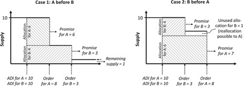
Eventually, both customers place an actual order for respectively 8 and 3 units. If customer A has the longer order lead time, i.e. orders first (left part of Figure 2), they only receive a promise of 6 units as 4 units are reserved for customer B, who finally only orders and receives 3 units. In this case, the overall service level equals 82% (as 9 out of the 11 ordered products delivered) and there is 1 unit of product left in inventory.

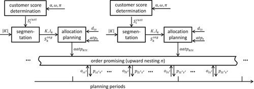
Figure 2. Rolling horizon scheme for customer ordering behaviour driven allocation planning.

If customer B has the longer order lead time and thus orders first (right part of Figure 2), they receive the ordered volume of 3 units. The remaining, unused supply allocated to customer B of 1 unit can still be used to fulfil part of customer A’s demand. This leads to a shipment of 7 units to customer A. The overall service level increases to 91% (as 10 out of the 11 ordered products delivered) and no inventory remains.

Clearly, this example shows that the contractual terms for the order lead times of different customers strongly affect key performance indicators such as service levels and inventory. This highly relevant problem has so far not been addressed in academic publications and is at the core of what we identify as the contract portfolio problem: the identification of a combination of contracts in a portfolio of customer contracts that allows to achieve high service levels with corresponding low inventory levels. The industry, however, still focuses on negotiating favourable terms in individual contracts missing out on the opportunities arising from a comprehensive portfolio perspective.

Our work has the following contributions: Firstly, we develop a framework that extends the demand fulfilment methodology of Seitz, Grunow, and Akkerman (2020). The novel methodology fosters a contract portfolio perspective by incorporating the differences in order lead time in the allocation methodology. It hereby enhances reallocation opportunities between customers such as outlined in the above example. Secondly, we demonstrate how to apply and parametrise the framework for real-world contract portfolios from the semiconductor sector. For our analysis, we elicit data for 10 different industry portfolios with different order-lead-time characteristics. Thirdly, our numerical analysis based on industry data shows that the consideration of order lead times results in significant improvements in service levels and performance robustness of contract portfolios. Finally, our numerical results show that contract portfolios in which order lead times and the accuracy of ADI are negatively correlated perform substantially better. They allow a more efficient reallocation of excess allocations. Such portfolios are even superior to portfolios in which all customers have long order lead times.

Our results have several managerial implications for companies operating in situations of supply shortage. Firstly, demand fulfilment approaches should not cluster customers in segments. Instead, they should allocate available supply to individual customers, considering the individual lead times in relation to lead times of other customers in the portfolio. Secondly, to achieve high service levels with corresponding low inventory levels, order lead times of a portfolio should be distributed such that longer order lead times are negotiated with customers providing ADI with lower accuracy. Finally, suppliers should initiate discussion on possibilities to increase ADI accuracy with customers with relatively short lead times, as this allows construction of contract portfolios with more efficient reallocation opportunities.

The remainder of this paper is organised as follows. Section 2 provides a literature review. In Section 3 we explain our framework for demand fulfilment in detail. Section 4 introduces a case from the semiconductor industry, describes the experimental design of our numerical study and presents its results. Finally, we conclude our paper with the implications of the results and an outlook on future research in Section 5.

2. Related literature

Our research is related to several streams of supply chain literature. First, the supply chain planning context we study is related to research on supply network planning approaches considering ADI. Secondly, our focus on contract portfolios relates to research on supply chain coordination with contracts. Finally, our focus on demand fulfilment relates to the literature developing mechanisms for these fulfilment processes. In the following, we will discuss each of these three literature streams in the context of our work.

In supply network planning approaches, there is often some consideration of ADI. Many authors have shown that ADI can reduce, but not eliminate, demand volatility and uncertainty in supply chains. This is also the case in most situations in which ADI is imperfect, but unbiased (e.g. Gayon, Benjaafar, and de Véricourt 2009; Bernstein and DeCroix 2015; Topan et al. 2018), even though the advantages depend on the quality of information (i.e. the level of imperfection of the ADI).

However, in shortage situations ADI is often not unbiased. Customers can strategically communicate ADI quantities higher than their actual demand forecast in the hope that this will increase their share in the allocation procedure. This behaviour, called rationing gaming, results in the risk of inefficient allocation decisions, demonstrated by low on-time service levels and high inventories positions due to excess allocations (see e.g. Lee, Padmanabhan, and Whang 2004). For this reason, suppliers need to install demand fulfilment methods that increase service levels in uncertain environments and incentivise customers to provide unbiased ADI. We propose one such method in this paper. Most publications in this field, however, study the influence of unbiased or biased ADI for given production control strategies (Karaesmen, Buzacott, and Dallery 2002; Claudio and Krishnamurthy 2009; Karrer, Alicke, and Günther 2012; Altendorfer and Minner 2014). What is often not considered, is that final customer orders often have different lead times (see also Seitz and Grunow 2017), and that this difference in the timing of ADI turning into actual orders has a large impact on the efficient allocation of capacities. As these ADI agreements and final order lead times are important parts of contracts in business-to-business settings, in this paper, we investigate the influence of the design of contract portfolios determining order lead times and ADI on the supply chain performance for a given demand fulfilment process.

In the literature on supply chain coordination with contracts, contracts coordinate the material, value, and information flows in decentrally planned supply chains. Cachon (2003) provides a broad overview, to which we refer for a more general discussion of the field. Tsay, Nahmias, and Agrawal (1999) classify contract clauses into eight categories. In relation to our work, the categories of quantity flexibility, lead times, and allocation rules are relevant.

In contracts setting quantity flexibility, the maximum allowed deviation of the ADI from the final order of a customer and according monetary penalties are determined for different ADI horizons. Contracts setting minimum order lead times for customers determine the minimum horizon with which a customer has to communicate a final order quantity to its supplier. The literature in these fields investigates the necessary conditions for supply chain partners to conclude such contracts and determines the optimal behaviour of supply chain partners for a given contractual relationship in order to study its effects on the overall supply chain performance and the distribution of risks within the supply chain (Iyer and Bergen 1997; Tsay 1999; Tsay and Lovejoy 1999; Barnes-Schuster, Bassok, and Anupindi 2006; Lutze and Özer 2008; Kim 2011; Kremer and Van Wassenhove 2014; Kim, Park, and Shin 2014; Knoblich, Heavey, and Williams 2015; Shen, Choi, and Minner 2019). The publications typically assume enough supply to fulfil the total of the demand of the customer and do not consider the possibility of a structural bias in the ADI information provided by the customer.

For supply shortage situations, as our study is concerned with, contracts require supply allocation rules, i.e. agreements on the process of distributing scarce supply between different customers. Publications on this topic typically investigate the effects of such rules on their suitability to coordinate the supply chain efficiently. Many of the studied allocation rules are based on the customer demand forecasts (i.e. the ADI). For instance, studies focus on the impact of incentivising customers to provide truthful ADI on increasing or decreasing overall profits, costs, stocks, and service levels (Cachon and Lariviere 1999a, 1999b; Plambeck and Taylor 2007; Huang, Chen, and Lin 2013; Xiao and Shi 2016).

In contrast to our research, which takes the perspective of the supplier, most of the reviewed publications aim at coordinating the supply chain globally by using game theoretical approaches. Apart from the work on allocation rules, the previous research focuses on dyadic contractual relationships between a supplier and a customer, for which it is decided which contract terms to include and how to set them. The same contract terms apply to all customers. An exception is Barnes-Schuster, Bassok, and Anupindi (2006), who determine order lead times for multiple customers minimising global supply chain cost. However, it is assumed that the supplier can always fill the total demand of customers within the contractual order lead time. Furthermore, the exchange of ADI is not considered in the publication.

In general, the effects of allocation rules, ADI terms, and order lead time contracts have been addressed in the contracting literature, but only separately, neglecting their interactions in the structure and dynamics of the demand fulfilment process.

Finally, our research is also related to the literature dealing with mechanisms for demand fulfilment, which can be categorised into the streams revenue management and demand fulfilment with advanced planning systems. Both categories essentially deal with the same supply chain processes (Quante, Meyr, and Fleischmann 2009). Revenue management concepts, however, typically do not reflect contractual terms between customer and supplier or address multi-period planning processes involving ADI, replenishment, and storage of supply.

Demand fulfilment approaches using advanced planning systems either process orders in batches or promise orders in real-time (see e.g. Ball, Chen, and Zhao 2004; Framinan and Leisten 2010). While batch order promising approaches allow prioritisation of customers, real-time order promising approaches require a preceding allocation planning mechanism that reserves certain quantities of supply to specific customers in case of supply shortage, to avoid suboptimal first come first served order promising (e.g. Meyr 2009). Since customers usually require an immediate response, real-time order promising approaches are more common in industrial environments. Common allocation planning approaches use rules (Cederborg and Rudberg 2009; Vogel and Meyr 2015; Kilger and Meyr 2015) or optimisation models based on linear programming (Ervolina et al. 2009; Meyr 2009; Chien, Wu, and Wu 2013; Chen and Dong 2014; Chiang and Hsu 2014; Lebreton 2015; Framinan and Perez-Gonzalez 2016; Cano-Belmán and Meyr 2019). As differences between ADI and final order quantities lead to inefficiencies in the supply allocation, recent work has also specifically addressed the modelling of release mechanisms and supply reallocation approaches (e.g. Esteso et al. 2018, 2019; Xu and Chen 2021).

For a case from an agri-food manufacturer, Papier (2016) shows that the usage of ADI in allocation planning to different markets can increase the expected profit significantly. In contrast to our approach, reallocation of supply is not possible in the approach. Furthermore, as we allocate supply to individual customers our framework is designed for a different level of aggregation. In Seitz, Grunow, and Akkerman (2020), a supply allocation approach is presented, which uses ADI bias and profitability information. The method increases customer service levels and counteracts rationing gaming by incentivizing customers to provide truthful ADI. A recent behavioural study by Pekgün et al. (2019) shows that such forecast-accuracy-based incentives do lead to improved forecasts.

In conclusion, none of the approaches discussed above account for customer order lead times and their possible heterogeneity, even though this can have significant impact on the efficiency of demand fulfilment processes. Considering the interaction between such heterogeneous customer-specific characteristics does however require looking at contract portfolios.

3. A flexible demand fulfilment framework for evaluation of ADI and order lead time contracts

In this section, we develop a new demand fulfilment framework, which we use as a testbed for industrial contract portfolios. The framework considers the contractual parameters set for each individual customer as well as the resulting customer forecasting and ordering behaviour. It extends the methodology presented in Seitz, Grunow, and Akkerman (2020) by (1) considering order lead times, (2) using a dynamic updating process for customer scoring to reflect changing customer ordering behaviour, and (3) adding flexibility to the supply allocation and order promising processes. Its processes are executed in a short-term rolling horizon fashion (e.g. every week).

Figure 2 provides an overview of our framework and includes the following notation (which will also be used later in this section to detail the individual processes in the framework).

$k\in K$	=	Set of customer segments
$i\in I_k$	=	Set of customers in segment k (subset of all customers $i\in I$)
$S_i^{\mathit{\text{cust}}}$	=	Customer score for customer i used in segmentation and demand fulfilment
α	=	The weight of ADI accuracy in calculating customer scores
$\omega$	=	The weight of order lead time in calculating customer scores
$\pi$	=	The weight of profitability in calculating customer scores
$S_k^{\mathit{\text{seg}}}$	=	Segment score for segment k used in demand fulfilment
n	=	Level of upward nesting allowed in during order promising
$d_{i\tau }$	=	Advance Demand Information (ADI) provided by customer i for period $\tau$
$at{p}_t$	=	Available-To-Promise (ATP) supply for period t
$aat{p}_{kt\tau }$	=	ATP supply available in period t allocated to segment k to cover demand in period $\tau$
$o_{i{\tau }^{\mathrm{\prime }}}$	=	Final customer order for customer i in period ${\tau }^{\mathrm{\prime }}$
$p_{i{t}^{\mathrm{\prime }}{\tau }^{\mathrm{\prime }}}$	=	Order promise for order $o_{i{\tau }^{\mathrm{\prime }}}$ in period $t^{\mathrm{\prime }}$

The segmentation and allocation planning are based on customer scores. Typically, this is a single score that most often reflects a customer’s importance based on profitability. This measure of profitability can have a short-term focus on the actual profit margin but can also include more strategic long-term considerations regarding future profitability. In this paper, in addition to profitability, order lead time and the accuracy of ADI is considered in the calculation of the customer score $S_i^{\mathit{\text{cust}}}$ for every individual customer $i\in I$ (see Section 3.1).

The customer segmentation process (Section 3.2) subsequently segments customers into a given number of $|K|$ segments $k\in K$ that, together with their respective segment score $S_k^{\mathit{\text{seg}}}$, are used in the allocation planning and order promising processes.

In the allocation planning (Section 3.3), the available-to-promise (ATP) supply $at{p}_t$ becoming available at the beginning of planning time period t is allocated to the customer segments k. This allocation is based on ADI demands $d_{i\tau }$ of the customers i as forecasted for period $\tau$. Note that we use the indices t and $\tau$ to distinguish between the time points related to supply (t) and the time points related to the customer demands ($\tau$) (i.e. the time period in which the order must be ready). The resulting allocated available-to-promise (AATP) supply $aat{p}_{kt\tau }$ is used by a real-time order promising process to generate order promises $p_{i{t}^{\mathrm{\prime }}{\tau }^{\mathrm{\prime }}}$ for incoming orders $o_{i{\tau }^{\mathrm{\prime }}}$ for the individual customers $i\in I$. Here, the delivery period (supply) and the time period of the requested delivery date (demand) are denoted by indices $t^{\mathrm{\prime }}$ and ${\tau }^{\mathrm{\prime }}$.

Finally, the order promising step allows for so-called upward nesting in order to increase order promising flexibility (see also Section 3.4). The concept of nesting is often used in the context of prioritising customer segments, where the customers segments are considered to be nested hierarchically, i.e. customer segments with higher priority also have access to AATP of customer segments with lower priority (see also Kilger and Meyr 2015). Upward nesting then means that orders can not only consume AATP quantities reserved for customers segments with lower priority, but additionally, allocations of a limited number of $n$ customer segments with higher priority can be consumed.

3.1. Customer score determination

Our customer score determination approach uses the normalised profitability $pro{f}_i^{norm}$, ADI accuracy ${\mathit{\text{acc}}}_i^{\mathit{\text{norm}}}$, and average order lead time ${\mathit{\text{olt}}}_i^{\mathit{\text{norm}}}$ of the customers to determine their priority in demand fulfilment.

The parameters ${\mathit{\text{prof}}}_i^{\mathit{\text{norm}}}$ and ${\mathit{\text{acc}}}_i^{\mathit{\text{norm}}}$ are respectively derived from data on individual customer profitability ${\mathit{\text{prof}}}_i^{}$ and data on the accuracy of ADI for each individual customer ${\mathit{\text{acc}}}_i^{}$. In Equations (1) and (2) below, ${\mathit{\text{prof}}}^{\mathit{\text{min}}}$ and ${\mathit{\text{prof}}}^{\mathit{\text{max}}}$ as well as ${\mathit{\text{acc}}}^{\mathit{\text{min}}}$ and ${\mathit{\text{acc}}}^{\mathit{\text{max}}}$ represent the minimum and maximum profitability and accuracy across all customers. (1) $\begin{array}{rl}{\mathit{\text{prof}}}_i^{\mathit{\text{norm}}}& =\frac{{\mathit{\text{prof}}}_i-{\mathit{\text{prof}}}_{}^{\mathit{\text{min}}}}{{\mathit{\text{prof}}}_{}^{\mathit{\text{max}}}-{\mathit{\text{prof}}}_{}^{\mathit{\text{min}}}}\end{array}$(1) (2) $\begin{array}{rl}{\mathit{\text{acc}}}_i^{\mathit{\text{norm}}}& =\frac{{\mathit{\text{acc}}}_i-{\mathit{\text{acc}}}_{}^{\mathit{\text{min}}}}{{\mathit{\text{acc}}}_{}^{\mathit{\text{max}}}-{\mathit{\text{acc}}}_{}^{\mathit{\text{min}}}}\end{array}$(2) The ADI accuracy ${\mathit{\text{acc}}}_i$ is derived from historical ADI and order data. Since we usually have a sufficiently large number of observations, we can use a regular t-test to assess whether or not the difference between ADI and order sizes is significantly different from zero. If it is not proven to be significantly different, we consider it to be a forecasting error and use an accuracy of 100%. If it is significantly different, this part of the forecasting error represents the customer’s strategic rationing gaming behaviour that is deducted from the accuracy. For instance, in case a customer’s ADI significantly exceeds their eventual orders by 15%, the accuracy measure for this customer is 85%.

To determine the average order lead time for each customer ${\mathit{\text{olt}}}_i$ and its normalised version ${\mathit{\text{olt}}}_i^{\mathit{\text{norm}}}$, Equations (3) and (4) below are used. The time period when an order o must be ready for delivery, i.e. the due date requested by the customer is denoted as $t_o^{\mathit{\text{due}}}$. The time period when the order $o$ was placed by the customer is represented by $t_o^{\mathit{\text{placed}}}$. The set $O_i$ contains all orders $o$ of customer $i$ in the past $t\in T^{\mathit{\text{past}}}$ time periods. Note that the ranges of order lead times for individual customers are normally not that wide, as these ranges are limited in the contracts the supplier closes with their customers. To normalise the average order lead times, we relate all of them to the full range of average order lead times defined by ${\mathit{\text{olt}}}^{\mathit{\text{min}}}=\underset{i}{min}{\mathit{\text{olt}}}_i$ and ${\mathit{\text{olt}}}^{\mathit{\text{max}}}=\underset{i}{max}{\mathit{\text{olt}}}_i$. (3) $\begin{array}{rl}{\mathit{\text{olt}}}_i^{}& =\frac{\sum _{o\in O_i}\left(t_o^{\mathit{\text{due}}}-t_o^{\mathit{\text{placed}}}\right)}{|O_i|}\end{array}$(3) (4) $\begin{array}{rl}{\mathit{\text{olt}}}_i^{\mathit{\text{norm}}}& =\frac{{\mathit{\text{olt}}}_i-{\mathit{\text{olt}}}_{}^{\mathit{\text{min}}}}{{\mathit{\text{olt}}}_{}^{\mathit{\text{max}}}-{\mathit{\text{olt}}}_{}^{\mathit{\text{min}}}}\end{array}$(4) The customer scores $S_i^{\mathit{\text{cust}}}$ are determined by Equation (5) below. The factors $\alpha$, $\omega$, and $\pi$ (with $\alpha +\omega +\pi =1$) determine the weight of the historical ADI accuracy, order lead time, and profitability of a customer in $S_i^{\mathit{\text{cust}}}$. (5) $S_i^{\mathit{\text{cust}}}=\alpha \cdot {\mathit{\text{acc}}}_i^{\mathit{\text{norm}}}+\omega \cdot {\mathit{\text{olt}}}_i^{\mathit{\text{norm}}}+\pi \cdot {\mathit{\text{prof}}}_i^{\mathit{\text{norm}}}$(5) The weights used can either be set according to managerial preferences or can be initialised based on historical data and a target performance measure. In this paper, we select the weights such that they lead to an optimal service level for a set of historical data (more details on this parametrization process are provided in Section 4).

The determination of customer scores based on the procedures described above requires more customer-specific data than used in previous literature. Customer profitability is often used in prioritisation of customers (see e.g. Kilger and Meyr 2015), but heterogeneity in ADI accuracy and order lead times is not commonly used (with the exception of the consideration of ADI accuracy by Seitz, Grunow, and Akkerman 2020). The implementation of the proposed procedure therefore also requires collecting and maintaining ADI accuracy data (e.g. based on historical performance) and order lead time data (e.g. extracted from contracts) for individual customers, as well as their integration into the IT systems used for allocation planning and order promising. However, in today’s industry settings, this type of data is readily available.

3.2. Customer segmentation

Customer segments allow for a pooling of allocated available-to-promise supply between different customers. Similar to Meyr (2009), our customer segmentation method uses the distance ${\mathit{\text{dist}}}_{ij}$ between two customers $i$ and $j$, which is defined as the absolute value of the difference of the customer scores (Equation (6)). (6) ${\mathit{\text{dist}}}_{ij}=|S_i^{\mathit{\text{cust}}}-S_j^{\mathit{\text{cust}}}|$(6) The customer segmentation model is described by Equations (7)–(12). With the decision variable $v_{ik}$, customer $i$ is assigned to segment $k$. The decision variable $\overline{w}$, called width, is the maximum distance between any two customers $i$ and $j$ belonging to the same customer segment.

Minimise (7) $z=\overline{w}$(7) subject to (8) $\begin{array}{rl}\sum _{k\in K}{v}_{ik}& =1\mathrm{\forall }i\in I\end{array}$(8) (9) $\begin{array}{rl}\overline{w}& \ge \left(v_{ik}+v_{jk}-1\right)\cdot {\mathit{\text{dist}}}_{ij}\mathrm{\forall }k\in K;i,j\in I:i<j\end{array}$(9) (10) $\begin{array}{rl}\sum _{i\in I}{v}_{ik}& \ge \frac{|I|+|K|-1}{2|K|-1}\mathrm{\forall }k\in K\end{array}$(10) (11) $\begin{array}{rl}{v}_{ik}& \in \left\{0,1\right\}\mathrm{\forall }k\in K,i\in I\end{array}$(11) (12) $\begin{array}{rl}\overline{w}& \ge 0\mathrm{\forall }k\in K\end{array}$(12)

The objective function (7) minimises $\overline{w}$, ensuring that the customer segment with the largest maximum ${\mathit{\text{dist}}}_{ij}$-value is as homogeneous regarding the customer scores $S_i^{\mathit{\text{cust}}}$ as possible. Constraint (8) ensures that each customer is assigned to exactly one segment. Constraint (9) states that $\overline{w}$ must be greater or equal to the distance between any two customers $i$ and $j$ belonging to the same segment (by multiplying with $\left(v_{ik}+v_{jk}-1\right)$, we ensure that no minimum is set for the width in case the customers are in different segments). Constraint (10) sets the minimum segment size to the value of $\frac{|I|+|K|-1}{2|K|-1}$, which is a value that ensures a reasonable spread of customers over segments, while also still leaving some flexibility in the segmentation (the expression is derived in Appendix). Here, without loss of generality, we assume that $|K|>1.$Constraint (11) and (12) define $v_{ik}$ as binary and $\overline{w}$ as non-negative.

After customer segmentation, the set of customer segments $K$, the sets $I_k$ containing the customers belonging to the segment $k$ and the segment scores $S_k^{\mathit{\text{seg}}}$ are provided to the allocation planning process. The segment scores are calculated with Equation (13), in which $v_{ik}^{\ast }$ are the optimal values of the decision variables $v_{ik}$. (13) $S_k^{\mathit{\text{seg}}}=\frac{\sum _{i\in I}\left(v_{ik}^{\ast }\cdot S_i^{\mathit{\text{cust}}}\right)}{\sum _{i\in I}{v}_{ik}^{\ast }}$(13) Note that if $|K|=|I|$, each customer segment contains only one customer and subsequent allocation planning and order promising will be performed on the level of individual customers.

3.3. Allocation planning model

The allocation planning process of our framework is a modification of the approach in Seitz, Grunow, and Akkerman (2020), which in turn was an adaptation of the approach by Meyr (2009). The model is built for situations in which demand exceeds supply and uses the customer segments described above. It is described by Equations (14)–(17).

Maximise (14) $\begin{array}{rl}z& =\sum _k\sum _{\tau }\left[\sum _t\left(S_k^{\mathit{\text{seg}}}\cdot aat{p}_{kt\tau }\right)-\sum _{t<\tau }\left(c_{t\tau }^e\cdot aat{p}_{kt\tau }\right)\right.\\ & \left.-\sum _{t>\tau }\left(c_{t\tau }^l\cdot aat{p}_{kt\tau }\right)\right]\end{array}$(14) subject to (15) $\begin{array}{rl}\sum _{t}aat{p}_{kt\tau }& \le \sum _{i\in I_k}{d}_{i\tau }\mathrm{\forall }k\in K,\tau \in T\end{array}$(15) (16) $\begin{array}{rl}\sum _k\sum _{\tau }aat{p}_{kt\tau }& =at{p}_t\mathrm{\forall }t\in T\end{array}$(16) (17) $\begin{array}{rl}aat{p}_{kt\tau }& \ge 0\mathrm{\forall }k\in K,t\in T,\tau \in T\end{array}$(17)

The objective function (14) maximises the segment-score-weighted supply allocations and penalises early and late demand fulfilment with the factors $c_{t\tau }^e$ and $c_{t\tau }^l$, which represent penalties for fulfilment of demand that was supposed to be fulfilled in period $\tau$ in period $t$ (and conditions $\tau <t$ and $\tau >t$ are used to distinguish early and late fulfilment). Typically, these penalty costs reflect the contractual terms and the company’s priorities regarding earliness and lateness of fulfilment (reflecting market requirements). The objective function ensures that demands of segments with high $S_k^{seg}$ values are satisfied with priority. Constraint (15) ensures that the generated AATP quantities do not exceed customer demand forecasts. Constraint (16) states that the sum of allocated supply quantities must equal the total available ATP quantities.

3.4. Order promising

For order promising, we use an adaptation of the model presented in Meyr (2009). The model, which is described by Equations (18)–(21), decides on the portions of allocated supply $x_{k{t}^{\mathrm{\prime }}}$, which become available in period $t^{\mathrm{\prime }}$ and are used to fulfil an order of $o_{i^{\ast }{\tau }^{\mathrm{\prime }}}$ product units from customer $i^{\ast }$ due in period ${\tau }^{\mathrm{\prime }}$.

Maximise (18) $\begin{array}{rl}z& =\sum _{k\in K_{i^{\ast }}}\left[\sum _{t^{\mathrm{\prime }}}\left(S_k^{\mathit{\text{seg}}}\cdot x_{k{t}^{\mathrm{\prime }}}\right)-\sum _{t^{\mathrm{\prime }}<{\tau }^{\mathrm{\prime }}}\left(c_{t^{\mathrm{\prime }}{\tau }^{\mathrm{\prime }}}^e\cdot x_{k{t}^{\mathrm{\prime }}}\right)\right.\\ & \left.-\sum _{t^{\mathrm{\prime }}>{\tau }^{\mathrm{\prime }}}\left(c_{t^{\mathrm{\prime }}{\tau }^{\mathrm{\prime }}}^l\cdot x_{k{t}^{\mathrm{\prime }}}\right)\right]\end{array}$(18) subject to (19) $\begin{array}{rl}\sum _{k\in K_{i^{\ast }}}\sum _{t^{\mathrm{\prime }}}{x}_{k{t}^{\mathrm{\prime }}}& \le o_{i^{\ast }{\tau }^{\mathrm{\prime }}}\end{array}$(19) (20) $\begin{array}{rl}{x}_{k{t}^{\mathrm{\prime }}}& \le \sum _{\tau }aat{p}_{k{t}^{\mathrm{\prime }}\tau }\mathrm{\forall }k\in K_{i^{\ast }},t^{\mathrm{\prime }}\in T\end{array}$(20) (21) $\begin{array}{rl}{x}_{k{t}^{\mathrm{\prime }}}& \ge 0\mathrm{\forall }k\in K_{i^{\ast }},t^{\mathrm{\prime }}\in T\end{array}$(21) As in the allocation planning, the objective function (18) maximises the segment-score-weighted supply allocations and penalises early and late demand fulfilment. Constraint (19) states that the sum of consumed supply must not exceed the ordered quantity. Constraint (20) ensures that the allocation quantities $aat{p}_{k{t}^{\mathrm{\prime }}\tau }$ are not exceeded and Constraint (21) defines the non-negativity of the decision variables.

The model allows nesting of customer segments. The segments from which customer $i^{\ast }$ is allowed to consume allocated supply are represented in the set $K_{i^{\ast }}$. This set contains all segments for which Equation (22) holds. It includes not only the segment of customer $i^{\ast }$ and lower priority segments, but also the possibility to use upward nesting by including $n$ higher-priority segments. The function $\text{RNK}$ maps the customer segments in descending order of their segment scores onto the ordinal scale $\left[1;|K|\right]$. The customer segment of the ordering customer is represented by $k^{\ast }$. (22) $\left[\text{RNK}\left(S_k^{\mathit{\text{seg}}}\right)+n\right]\ge \text{RNK}\left(S_{k^{\ast }}^{\mathit{\text{seg}}}\right)$(22) For example, this means that with an upward nesting possibility of 1 segment ($n=1$), a customer in segment $k^{\ast }=3$ would be allowed to consume allocated supply from segments 2 and up, but not from customer segment 1 (as lower numbers represent higher priority). In our numerical study, we do not allow fulfilment of orders before their due date. Therefore, the promises $p_{i{t}^{\mathrm{\prime }}{\tau }^{\mathrm{\prime }}}$ are calculated with Equation (23). (23) $\begin{array}{rl}{p}_{i^{\ast }{t}^{\mathrm{\prime }}{\tau }^{\mathrm{\prime }}}& =\left\{\begin{array}{cc}0& \mathrm{\forall }{t}^{\mathrm{\prime }}\in T|t^{\mathrm{\prime }}<{\tau }^{\mathrm{\prime }}\\ \sum _{k\in K_{i^{\ast }}}\sum _{t^{\mathrm{\prime }}\in T|t^{\mathrm{\prime }}\le {\tau }^{\mathrm{\prime }}}{x}_{k{t}^{\mathrm{\prime }}}& \mathrm{\forall }{t}^{\mathrm{\prime }}\in T|t^{\mathrm{\prime }}={\tau }^{\mathrm{\prime }}\\ \sum _{k\in K_{i^{\ast }}}{x}_{k{t}^{\mathrm{\prime }}}& \mathrm{\forall }{t}^{\mathrm{\prime }}\in T|t^{\mathrm{\prime }}>{\tau }^{\mathrm{\prime }}\end{array}\right.\end{array}$(23)

4. Performance analysis of contract portfolios from the semiconductor industry

In this section, we analyse different customer contract portfolios using data from a large European company in the semiconductor industry. Typical for this industry (see also Mönch, Uzsoy, and Fowler 2018), the company operates in a business-to-business environment using contractual agreements with relatively large customers that use the semiconductors in e.g. automotive electronics, consumer electronics, and industrial equipment The contract portfolios are selected from this companies’ product range in a way that the resulting customer ordering behaviour shows different correlations of the length of the order lead time and the accuracy of ADI in the customer set. Selecting contract portfolios with these different correlations allows us to study the impact of order lead times in different circumstances.

After introducing our design of experiments in Section 4.1 we parametrise our demand fulfilment framework in Section 4.2. In Section 4.3, we perform a numerical analysis on the impact of exact parametrization of our approach, compare its performance to other demand fulfilment methodologies and analyse the influence of different contract portfolio designs on the demand fulfilment performance.

4.1. Assumptions, performance measures, and contract portfolios

We implement our approach as shown in Figure 2. The following two assumptions are made to eliminate all sources of uncertainty other than ADI bias:

• ATP quantities are deterministic.

• Orders will not be cancelled or rescheduled by customers once they enter the system.

Furthermore, we make two assumptions on the demand fulfilment processes:

• Orders can be fulfilled partially and with multiple shipments.

• If a part of an order cannot be promised when it is received, this part is lost.

We measure the effect of the design of contract portfolios on the demand fulfilment performance in order to derive insights for portfolio management. The indicator we choose is the on-time service level (OTSL), for which we use Equation (24). (24) $\text{OTSL}=\frac{\sum _{i\in I}\sum _{\tau \in T}{p}_{i\tau \tau }}{\sum _{i\in I}\sum _{\tau \in T}{o}_{i\tau }}$(24) Here, both time indices used in the numerator are set equal to $\tau$, as the delivery period and the time period of the requested delivery date are the same for on-time deliveries.

Our dataset contains 78 weeks of ADI for 143 customers and the corresponding 1644 orders for 10 products that each have their own portfolio of contracts: P1, … , P10 (Table 1). The design of the contract portfolio differs for all products. As a result, the length of the order lead time and the accuracy of ADI $\left({\mathit{\text{acc}}}_i\right)$ show different correlations $r\left({\mathit{\text{olt}}}_i,{\mathit{\text{acc}}}_i\right)$ for all products. Furthermore, the demand data for all 10 products differs in its predictive quality, i.e. the degree to which the future customer ADI accuracy can be predicted from the past. To measure the predictive quality of data, we use the average error ${\overline{\mathit{\text{err}}}}^{\mathit{\text{acc}}}$ of the ADI accuracy ${\mathit{\text{acc}}}_i^{}$ (Equation (25)). It calculates the average of the actual error in every period $t$. Here, ${\mathit{\text{acc}}}_i^{\mathit{\text{norm}}}\left(t\right)$ is the (normalised) actual accuracy of customer $i$ in period $t$ and ${\mathit{\text{acc}}}_i^{\mathit{\text{norm}}}$ is the (normalised) accuracy of customer $i$ calculated with historical demand data. To calculate ${\mathit{\text{acc}}}_i^{\mathit{\text{norm}}}$, a history of 30 periods before $t$ is used. Smaller values of ${\overline{\mathit{\text{err}}}}^{\mathit{\text{acc}}}$ indicate a higher predictive quality of data. In the remainder, we use the term contract portfolio as a synonym for a product of the dataset. (25) ${\overline{\mathit{\text{err}}}}^{\mathit{\text{acc}}}=\frac{\sum _{i\in I}\sum _{t=53}^{78}|{\mathit{\text{acc}}}_i^{\mathit{\text{norm}}}-{\mathit{\text{acc}}}_i^{\mathit{\text{norm}}}\left(t\right)|}{|I|\cdot |T|}$(25)

Table 1. Contract portfolios for numerical case study.

	P1	P2	P3	P4	P5	P6	P7	P8	P9	P10	Total
Customers	16	12	13	13	16	14	14	16	15	14	143
Orders	105	98	131	136	197	185	153	210	214	215	1644
Average ${\overline{\mathit{\text{acc}}}}_i$	85%	79%	82%	93%	91%	88%	68%	87%	91%	99%	86%
Average ${\mathit{\text{olt}}}_i$	2.20	3.38	3.07	1.87	1.47	3.44	2.98	2.82	3.15	2.98	2.73
Average ${\overline{\mathit{\text{err}}}}^{\mathit{\text{acc}}}$(in-sample)	0.03	0.19	0.27	0.31	0.41	0.38	0.40	0.44	0.51	0.65	0.36
Average ${\overline{\mathit{\text{err}}}}^{\mathit{\text{acc}}}$(out-of-sample)	0.04	0.21	0.29	0.30	0.38	0.39	0.40	0.46	0.48	0.59	0.35
$r\left({\mathit{\text{olt}}}_i,{\mathit{\text{acc}}}_i\right)$	0.28	−0.42	−0.18	0.43	0.05	−0.39	0.11	−0.03	0.32	0.23	0.04

In our numerical study, we use the weeks 31–52 of the data set to parametrise our approach (in-sample). This parametrisation is used to determine the service-level optimal levels for $\alpha$, $\omega$, and $\pi$, the key parameters used in the scoring of customers. Our experiments are then conducted on the weeks 53–78 of the dataset (out-of-sample). The weeks 1–30 are used to initialise ${\mathit{\text{acc}}}_i^{\mathit{\text{norm}}}$. Table 1 presents the ${\overline{\mathit{\text{err}}}}^{\mathit{\text{acc}}}$ values calculated on the in-sample and the out-of-sample data.

For confidentiality reasons, the real profitability of the customers is not provided in our dataset. However, we do have information on the relation of profitabilities of the customers within the dataset. For our numerical study, we represent the per-piece profitabilities of the most and least profitable customers with 0.1€ and 0.067€, which resembles a realistic relation between customer profitabilities in the semiconductor industry. Also based on industrial data, we further set the level of supply shortage to 20%, i.e. the total demand of all customers exceeds the available ATP for every product by 20%. We use the same level for all products to make the results for the portfolios comparable. This level is typical for the semiconductor manufacturer from which the portfolio data originates. To generate the supply values, the average cumulated demand of always five periods is calculated and multiplied with 0.8. The result is taken as the ATP supply in the respective weeks.

The numerical study is implemented in Java. IBM ILOG CPLEX V12.6.0 is used to solve the customer segmentation, allocation planning, and order promising models. The study was performed on a personal computer with an Intel Xeon E7-4860 v2 processor with 2.6 GHz and 32GB RAM on a 64-bit Microsoft Windows 7 installation.

4.2. Framework parametrisation

Before we can investigate the influence of the design of the customer contract portfolio on the demand fulfilment performance, we need to parametrise our demand fulfilment framework. For this, we use a full factorial design of experiments on the first 52 weeks of our dataset, as described in the previous section. For the number of customer segments, we use the values $\left\{2;4;6;|I|\right\}$ for $|K|$. The upward nesting level is varied between 0 and $|I|$ (as the number of customers provides an upper bound for the number of segments) and the weights of $\alpha$ and $\omega$ between 0 and 1 in 10 equidistant steps (with $\pi$ automatically resulting).

Table 2 presents the OTSL resulting for the different values of $|K|$ at the service level-optimal relative weights of $\alpha$ and $\omega$ and an upward nesting level of 0. Only for P10 showing exceptionally low predictive quality of demand data (${\overline{\mathit{\text{err}}}}^{\mathit{\text{acc}}}=0.65$), it is better to aggregate customers into segments. However, the size of these segments lies between two and three customers, which is much smaller than the segment size used in conventional demand fulfilment approaches (e.g. Meyr 2009). The reason for this is that in our B2B setting, the number of customers is small and sufficient information on customer-specific ADI accuracy is available. The table shows that for all other portfolios the service level-optimal number of customer segments equals the number of customers. This shows that our approach allows an efficient reallocation of available supply exploiting customer-specific information and does not have to rely on the pooling effect of segmentation. Only when the predictive quality of the data is low, segmentation may be useful.

Table 2. On-time service levels per ADI accuracy error and number of customer segments.

	P1	P2	P3	P4	P5	P6	P7	P8	P9	P10
${\overline{\mathit{\text{err}}}}^{\mathit{\text{acc}}}$	0.03	0.19	0.27	0.31	0.41	0.38	0.40	0.44	0.51	0.65
|K| = 2	23%	31%	35%	22%	31%	25%	28%	29%	23%	28%
|K| = 4	24%	33%	35%	24%	31%	26%	32%	32%	25%	35%
|K| = 6	28%	34%	39%	25%	35%	29%	33%	34%	28%	37%
|K| = |I|	35%	41%	43%	29%	42%	33%	37%	37%	29%	31%

If upward nesting is allowed ($n>0$), then the results are even more in favour of not combining customers into segments. This is because upward nesting reduces the advantage of segmentation by adding flexibility in order promising also for allocation planning on customer-individual level.

The maximum OTSL in Table 2 for all contract portfolios is approximately 40%. These rather low values result from the experimental design. The distribution of ATP is not aligned with the distribution of the requested delivery dates of customer orders, the customer segments are nested, and the total customer demand exceeds the total available supply significantly by 20%.

Consequently, early incoming orders consume large parts of the supply becoming available in later time periods. Hence, most of the later incoming orders cannot be promised on time. The theoretical maximum of 80% would be achieved, if all supply would be available already at the beginning of the experiment and the ADI and, hence, the AATP would be unbiased.

Figure 3(a) shows the average difference in OTSL over all contract portfolios and the average difference in OTSL for the contract portfolios with the lowest and highest ${\overline{\mathit{\text{err}}}}^{\mathit{\text{acc}}}$ (values of 0.03 and 0.65) for different levels of $\frac{n}{|I|}$. The x-axis thus represents increasing upward nesting possibilities, with $\frac{n}{|I|}=1$ representing full upward nesting, and thus a first-come-first-served (FCFS) approach in order promising. All figures are shown relative to the OTSL at an upward nesting level of $n=0$ and at the optimal levels for $\alpha$ and $\omega$.

Figure 3. (a) Relative difference in on-time service level by upward nesting level, (b) relative service level-optimal upward nesting level by error of ADI accuracy.

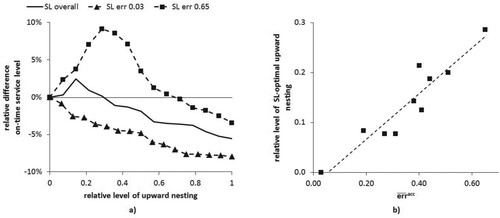
For all contract portfolios, the OTSL increases up to a certain level of $n$ and decreases monotonically for higher values of $n$. For high $n$ the OTSL falls below the OTSL without upward nesting. The reason for the increase of the service level for small $n$ is that errors in customer accuracy values can be compensated in the order promising process. However, with further increasing $n$ and a move towards the FCFS approach, service levels are decreasing. Seitz, Grunow, and Akkerman (2020) already show that an FCFS order promising leads to lower service levels than allocation planning based demand fulfilment.

Figure 3(b) presents the relative service level-optimal upward nesting level $\frac{n}{|I|}$ for the ${\overline{\mathit{\text{err}}}}^{\mathit{\text{acc}}}$-values of the contract portfolios investigated. It shows that the choice of $n$ depends on the predictive quality of data. For low values of ${\overline{\mathit{\text{err}}}}^{\mathit{\text{acc}}}$ the optimal $n$ is smaller than for high values.

For the service-level-optimal values of $n$ and $|K|$, Figure 4 shows the average relative difference of the OTSL relative to the case when $\alpha$ and $\omega$ are set to 0 for different levels of $\alpha$ and $\omega$. The average is taken over all 10 investigated portfolios. The figure illustrates that, for the in-sample data, the OTSL can be increased significantly (44% at the maximum) when customer order lead times and the accuracy of ADI of the customers are taken into account. In Section 4.3, we investigate, if such benefits also exist for out-of-sample data.

Figure 4. Average on-time service level performance of contract portfolios.

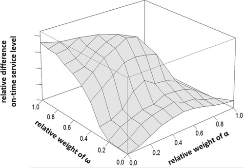
Table 3 shows the service-level-optimal $\alpha$, $\omega$, and $\pi$ levels for all 10 contract portfolios separately. It shows that with decreasing predictive quality of ADI data, customer order lead times get emphasised more in the customer scores. In other words, the service-level-optimal $\omega$ increases with increasing ${\overline{\mathit{\text{err}}}}^{\mathit{\text{acc}}}$. Therefore, it is important to know the predictive quality of data in order to be able to determine the correct values of $\alpha$, $\omega$, and $\pi$.

Table 3. Service-level-optimal weight factors.

	P1	P2	P3	P4	P5	P6	P7	P8	P9	P10
${\overline{\mathit{\text{err}}}}^{\mathit{\text{acc}}}$	0.03	0.19	0.27	0.31	0.41	0.38	0.40	0.44	0.51	0.65
$\alpha$	0.6	0.5	0.4	0.5	0.4	0.4	0.3	0.2	0.1	0.0
$\omega$	0.4	0.4	0.6	0.4	0.5	0.6	0.7	0.8	0.8	1.0
$\pi$	0.0	0.1	0.0	0.1	0.1	0.0	0.0	0.0	0.1	0.0

The impact of the parameter variations on profit is small. Compared to a profit-optimal parametrisation, the profit only declines by an average of 0.19%, when using the service-level-optimal parameters. For our out-of-sample numerical experiments, we therefore use the service-level-optimal parameters.

4.3. Numerical results

In the following, we investigate the demand fulfilment performance of our framework and derive insights on how to design contract portfolios for the set of customers. For this, we use the parameters determined in Section 4.2 and run our framework using the last 26 weeks of data in our datasets.

4.3.1. Impact of parametrisation

In this section, we determine the importance of individual, portfolio-specific parametrisation of our framework and draw conclusions on its ease of implementation. Here, individual, portfolio-specific parametrisation means that parameters are determined for each portfolio individually, as opposed to using the same parameter setting across all portfolios.

Table 4 shows the OTSL resulting from different levels of exact parametrisation. The second row of the table shows, which parameters are set to the exact values determined in Section 4.2. The parameters that are not shown in row 2 are set to the average of the exact values over all 10 datasets.

Table 4. Impact of portfolio-specific parametrisation.

	OTSL
	–	$\alpha \text{,}\omega \text{,}\pi$	$\alpha \text{,}\omega \text{,}\pi \text{,}\left|K\right|$	$\left|K\right|\text{,}n$	$\alpha \text{,}\omega \text{,}\pi \text{,}n$	$\alpha \text{,}\omega \text{,}\pi \text{,}n\text{,}\left|K\right|$
P1	32.2%	34.7%	34.7%	34.2%	35.9%	35.9%
P2	40.2%	41.0%	41.0%	40.6%	41.8%	41.8%
P3	43.2%	43.2%	43.2%	43.9%	43.9%	43.9%
P4	31.6%	33.1%	33.1%	31.6%	33.1%	33.1%
P5	42.9%	43.7%	43.7%	42.9%	43.7%	43.7%
P6	40.3%	40.3%	40.3%	40.3%	40.3%	40.3%
P7	36.4%	38.2%	38.2%	36.4%	38.2%	38.2%
P8	38.7%	40.7%	40.7%	40.9%	41.3%	41.3%
P9	34.0%	34.5%	34.5%	34.7%	35.4%	35.4%
P10	29.7%	32.3%	34.5%	35.4%	33.2%	36.2%
Average	36.9%	38.2%	38.4%	38.1%	38.7%	39.0%

The table illustrates that portfolio-specific parametrisation (i.e. the last column) consistently leads to the highest OTSL. Comparing the values to the in-sample results in Table 2 shows that the usage of our framework on out-of-sample data leads to equally good results. In other words, the parametrisation of our approach robustly leads to good results also for out-of-sample data.

Table 4 further shows that using average values for the parameters on average results in reasonable performance of the approach. This would make implementation easy. However, portfolio-specific parametrisation would further improve the performance of the approach, as the difference between the OTSL resulting from portfolio-specific parametrisation and the OTSL resulting from parametrisation with averages can be significant (as, e.g. for P10, where an increase from 29.7% to 36.2% is observed).

We conclude that where possible, portfolio-specific values for $n$, $\left|K\right|$, $\alpha$, $\omega$ and $\pi$ should be used. As Section 4.2 shows, this has to be done based on historical data and in dependence of the predictive quality of ADI; i.e. ${\overline{\mathit{\text{err}}}}^{\mathit{\text{acc}}}$.

4.3.2. Performance analysis of proposed demand fulfilment methodology

Previous work has primarily used profitability in demand fulfilment mechanisms. Some recent research also considered ADI accuracy. The sole consideration of profitability and/or ADI accuracy is a special case of our approach. In this section we measure the performance of our framework in relation to this previous work and determine the value of considering order lead times.

Table 5 compares our approach of using a combination of profitability, ADI accuracy, and order lead time as allocation criteria to an exclusive consideration of either profitability or ADI accuracy. Table 5 shows the OTSL of our framework, when only profitability is considered ($\pi =1$), ADI accuracy is considered ($\alpha =1$), only order lead times are considered ($\omega =1$), and when all parameters are taken into account (all). For all scenarios, the values of the parameters $n$ and $|K|$ are set to the service-level-optimal values determined in Section 4.2.

Table 5. The value of considering order lead time, ADI accuracy and profitability in demand fulfilment.

	OTSL
	$\pi =1$	$\alpha =1$	$\omega =1$	All
P1	25.6%	28.7%	35.1%	35.9%
P2	26.8%	29.9%	37.3%	41.8%
P3	27.8%	31.2%	38.5%	43.9%
P4	26.3%	25.9%	32.1%	33.1%
P5	26.1%	30.5%	39.8%	43.7%
P6	28.9%	28.2%	37.0%	40.3%
P7	28.3%	28.5%	36.6%	38.2%
P8	24.5%	27.1%	37.2%	41.3%
P9	26.6%	26.4%	35.0%	35.4%
P10	27.0%	26.1%	35.8%	36.2%

Table 5 shows that considering all parameters of the framework consistently leads to the highest OTSL values. Only considering profitability or ADI accuracy leads to relatively low OTSL for all 10 portfolios. Taking only order lead times into account leads to a significant increase of OTSL when compared to only considering profitability or ADI accuracy. For the portfolios showing low predictive quality of data, only considering order lead times results in good OTSL values also compared to the case making use of all parameters.

Our analysis shows that taking order lead times into account has a high positive influence on the performance of the demand fulfilment process. This is because it allows prioritising customers with long order lead times in the allocation planning step. When their orders realise, excess allocations resulting from biased ADI can be redistributed without loss of OTSL because other customers place their orders later. The additional consideration of ADI accuracy reduces the risk of excess allocations and leads to even higher performance, if the predictive quality of historical ADI accuracy values is high enough.

4.3.3. Dependence of customer service levels on the design of contract portfolios

This section draws conclusions on how contract portfolios should be designed such that the resulting interdependencies of the length of customer order lead times and the accuracy of ADI maximise the overall OTSL of the supplier. For the analysis, we run our demand fulfilment framework on the last 26 weeks of our dataset, using the parametrisation determined in Section 0.

Figure 5(a) shows the OTSL of the 10 portfolios in dependence of the average customer order lead time of the portfolios. The linear regression function evaluating the strength of the correlation of the length of the average customer order lead times and the resulting OTSL is shown as a dotted line. Its $R^2$ value of 0.00 shows that the two measures do not correlate. This is especially interesting because practitioners often solely focus on the negotiation of long order lead times with their customers. Figure 5(a), however, demonstrates that the length of the order lead time alone does not determine the OTSL.

Figure 5. On-time service level in dependence of (a) the average customer order lead time; (b) the correlation of order lead time and advance demand information bias.

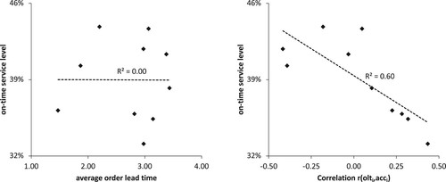
Figure 5(b) shows the OTSL of the 10 portfolios in dependence of the correlation $r\left({\mathit{\text{olt}}}_i,{\mathit{\text{acc}}}_i\right)$ between order lead times and ADI accuracy. If $r\left({\mathit{\text{olt}}}_i,{\mathit{\text{acc}}}_i\right)$ is positive, customers with long order lead times provide more accurate ADI than customers with shorter order lead times and vice versa.

Figure 5(b) shows better OTSL when order lead times and ADI accuracy are negatively correlated. Further, the OTSL grows with the strength of the correlation. The linear regression function (dotted line) illustrates this negative correlation of $r\left({\mathit{\text{olt}}}_i,{\mathit{\text{acc}}}_i\right)$ and OTSL. Its $R^2$ value of 0.60 indicates that it describes the relation well.

A negative $r\left({\mathit{\text{olt}}}_i,{\mathit{\text{acc}}}_i\right)$ leads to high OTSL values because ADI-bias-caused excess allocations for customers with long order lead times can be reallocated to customers with shorter order lead times but more accurate ADI. The redistributed supply allocations are less likely to be excessive because the ADI of the customers to which the supply is allocated is more accurate. Hence, the utilisation of the available supply as well as the overall OTSL are improved.

We therefore conclude that it is more important to design contract portfolios such that order lead times and ADI accuracy are negatively correlated than to maximise the average order lead times. Also, our results suggest that efforts to increase accuracy should focus on customers with short lead times, as this would enable a more efficient reallocation process.

5. Managerial implications and conclusion

When supply is short, the focus of the supply chain planning processes of the supplier and the advance demand information (ADI) of the customers shifts to demand fulfilment. In this process, the maximum supply output of the chain is distributed to the customers by means of customer segmentation, supply allocation planning, and order promising.

In this research, we analyse industrial contract portfolios with customer-specific terms for order lead times and ADI accuracy in order to derive insights for contract portfolio management. For this purpose, we investigate different portfolio designs in the dynamic context of industrial planning processes, for which we develop a framework that captures the interrelationship between order lead times and ADI accuracy. As such, the approach extends previous literature by not only taking profitability and accuracy of ADI of individual customers into account, but also specifically considering that different customer can have different order lead times. The consideration of customer-specific lead times is essential for efficient demand fulfilment processes. In order to reflect changing customer ordering behaviour, we use a dynamic process to continuously update customer data. If the ordering behaviour is hard to represent accurately for individual customers, we either allow for upward nesting in order promising to increase the flexibility of the approach or dynamically group customers into segments.

In a numerical study, we first demonstrate how to set up the framework for different contract portfolios in our semiconductor industry setting. We show that demand fulfilment should take all contract terms, including order lead times and historical forecasting and ordering behaviour of all customers into account, that it should be performed on the individual customer level, and that it is of special importance to determine the predictive quality of ADI in order to be able to parametrise our framework right. Furthermore, the analysis illustrates that our framework leads to significant improvements in service levels and robustness in performance.

Second, we derive insights aiding suppliers in their contract portfolio management. Our analysis shows that demand fulfilment performance is not primarily determined by the absolute length of the order lead times but by the presence of a negative correlation with the accuracy of advance demand information in the entire contract portfolio. Then, excess allocations can be re-allocated to other customers without loss of service levels. Consequently, suppliers should consider the portfolio of all customers and negotiate relatively long order lead times for customers showing relatively low accuracy of advance demand information. Alternatively, suppliers could initiate a discussion on ADI accuracy with customers with relatively short lead times, with the aim of increasing their ADI accuracy and establishing a more efficient allocation process by improving the reallocation opportunities. These insights also help focus the attention of customer relations resources in efforts to achieve the best possible service levels and resource allocations in situations with supply shortage.

Previous research also studied the use of supply reallocation to increase the efficiency of allocation processes in which differences between ADI and final order quantities exist (e.g. Esteso et al. 2018, 2019; Xu and Chen 2021). Previous work (Pekgün et al. 2019; Seitz, Grunow, and Akkerman 2020) also shows that suitable allocation processes can incentivize customers to provide truthful ADI, which reduces inefficiencies. However, none of these previous studies specifically addresses the impact of order lead time agreements on reallocation. The results presented in this paper show that a portfolio perspective on contracts with heterogeneous lead times significantly increases the efficiency of the allocation process. As long as the predictive quality of the historical data is sufficient, the demand fulfilment process does not even have to rely on pooling effect of segmentation extensively studied in previous research (e.g. Meyr 2009).

It should be noted that the allocation planning and order promising approaches are executed on the level of individual products. Depending on product and market characteristics, this also allows different parametrisation for different products. Our approach assumes that different customers demand the same product. For highly customised products our approach has to be applied to more generic semi-finished products used for multiple customers.

In situations where the supply shortage is transient, the allocation planning and order promising procedures can be kept in place when companies move in and out of supply shortage situations. This is beneficial because (1) it avoids having to reconfigure the planning systems used for the demand fulfilment procedures, and (2) it allows for a faster response when a company moves into a shortage situation again.

For future research, considering additional data in demand fulfilment activities is interesting. For example, substitution of products taking into account the individual willingness of customers to substitute has not been dealt with so far. Also, including uncertainty of supply and volatility of demand after order realisation is a further extension possibility. Moreover, further investigating the interactions between supply network planning, demand fulfilment, and customer contracting is an interesting direction of further research. In many industries, production quotas for supply planning are negotiated between different business divisions of a company. For example, efforts could be spent on integrating this type of allocation with supply allocation for customers taking contracts into account and streamlining all these activities in a holistic approach aiming at the maximisation of customer service levels and profits, in collaboration between supply chain planning and contracting departments.

Disclosure statement

No potential conflict of interest was reported by the author(s). An early version of this paper was included in the PhD thesis of the first author (Seitz 2017).

Additional information

Notes on contributors

Alexander Seitz

Alexander Seitz is heading Planning and Supply Chain Excellence at the Power & Sensor Systems Division of Infineon Technologies. He graduated from the Technical University of Munich with a PhD in Industrial Engineering and a Dipl.-Ing. in Mechanical Engineering. His research interests are in semiconductor operations management with a focus on data-driven approaches to increase profitability, scalability, robustness, and customer service levels of industrial demand fulfilment.

Renzo Akkerman

Renzo Akkerman is an Associate Professor in Operations Research and Logistics at Wageningen University in The Netherlands. Earlier, he was a Professor in Operations Management and Technology at the Technical University of Munich in Germany and an Associate Professor in Operations Management at the Technical University of Denmark. He graduated from the University of Groningen in The Netherlands with a PhD in Operations Management and an MSc in Econometrics and Operations Research. His (often interdisciplinary) research mostly deals with operations management in process industries, with topics ranging from planning and scheduling to supply chain design.

Martin Grunow

Martin Grunow is a Professor of Production and Supply Chain Management at the Technical University of Munich’s TUM School of Management in Germany. He received his MSc degree in Industrial Engineering and his PhD from Technical University Berlin. After working in the R&D department of Evonik Degussa, Martin was a Full Professor of Operations Management and Department Head at Technical University of Denmark. In his research, he develops analytics methodology for manufacturing and logistics. Martin has a special interest in the electronics and automotive sector as well as in the process industries, including chemicals, pharmaceuticals, and food.

Appendix. Minimum segment size

In our customer segmentation model, we set the minimum segment size $s^{\mathit{\text{min}}}$ to a value that aims at achieving a trade-off between balanced segment sizes and flexibility in segmentation. To achieve this, we set $s^{\mathit{\text{min}}}$ such that a prioritised sequence of customers $S$ would have at least $\left(s^{\mathit{\text{min}}}-1\right)$ unassigned customers between the $|K|$ segments of size $s^{\mathit{\text{min}}}$ if these were formed as evenly positioned along the sequence $S$ as possible. For $|I|=9$ customers and $|K|=3$ segments, this would for instance hold for a minimum segment size $s^{\mathit{\text{min}}}=2$, as illustrated in (A1) below. (A1) $S=\left\{\left(12\right)34\left(56\right)7\left(89\right)\right\}$(A1)

For $|I|=20$ customers and $|K|=4$ segments, it would hold for a minimum segment size $s^{\mathit{\text{min}}}=3$, leaving in total 8 customers to be assigned.

To formulate this in general, the above-mentioned principle means that the customers would get divided in $|K|$ segments of size $s^{\mathit{\text{min}}}$, and $|K-1|$ unassigned sets of customers with a set size of at least $\left(s^{\mathit{\text{min}}}-1\right).$ From this, it follows that (A2) $|K|\cdot s^{\mathit{\text{min}}}+\left(|K|-1\right)\cdot \left(s^{\mathit{\text{min}}}-1\right)\le |I|$(A2)

Rewriting this inequality as a condition on $s^{\mathit{\text{min}}}$ leads to (A3) $s^{\mathit{\text{min}}}\le \frac{|I|+|K|-1}{2|K|-1}$(A3)

This means that the largest possible integer value for $s^{\mathit{\text{min}}}$ that would still satisfy this condition would be (A4) $\frac{|I|+|K|-1}{2|K|-1}$(A4) which we can then use this as the minimum segment size in our work. Note that the example given in (A1) is only used to motivate the derivation of the minimum segment size. The general condition may lead to very different clusters. For example: (A5) $S=\left\{\left(12\right)\left(34\right)\left(56789\right)\right\}$(A5)

In situations in which a single customer makes up most of the sales volume, our minimum-segment-size approach might not be appropriate, and an alternative approach can and should be used.

References

- Altendorfer, K., and S. Minner. 2014. “A Comparison of Make-to-Stock and Make-to-Order in Multi-Product Manufacturing Systems with Variable Due Dates.” IIE Transactions 46 (3): 197–212. doi: https://doi.org/10.1080/0740817X.2013.803638
- Ball, M. O., C.-Y. Chen, and Z.-Y. Zhao. 2004. “Available to Promise.” In Handbook of Quantitative Supply Chain Analysis, edited by D. Simchi-Levi, D. D. Wu, and Z.-J. Shen, 447–483. New York: Springer.
- Barnes-Schuster, D., Y. Bassok, and R. Anupindi. 2006. “Optimizing Delivery Lead Time/Inventory Placement in a Two-Stage Production/Distribution System.” European Journal of Operational Research 174 (3): 1664–1684. doi: https://doi.org/10.1016/j.ejor.2002.08.002
- Bernstein, F., and G. A. DeCroix. 2015. “Advance Demand Information in a Multiproduct System.” Manufacturing & Service Operations Management 17 (1): 52–65. doi: https://doi.org/10.1287/msom.2014.0502
- Cachon, G. P. 2003. “Supply Chain Coordination with Contracts.” In Handbooks in Operations Research and Management Science. Vol. 11., edited by A. G. de Kok and S. C. Graves, 227–339. Amsterdam: Elsevier.
- Cachon, G. P., and M. A. Lariviere. 1999a. “Capacity Allocation Using Past Sales: When to Turn-and-Earn.” Management Science 45 (5): 685–703. doi: https://doi.org/10.1287/mnsc.45.5.685
- Cachon, G. P., and M. A. Lariviere. 1999b. “Capacity Choice and Allocation: Strategic Behavior and Supply Chain Performance.” Management Science 45 (8): 1091–1108. doi: https://doi.org/10.1287/mnsc.45.8.1091
- Cano-Belmán, J., and H. Meyr. 2019. “Deterministic Allocation Models for Multi-Period Demand Fulfillment in Multi-Stage Customer Hierarchies.” Computers & Operations Research 101: 76–92. doi: https://doi.org/10.1016/j.cor.2018.09.002
- Cederborg, O., and M. Rudberg. 2009. “Customer Segmentation and Capable-to-Promise in a Capacity Constrained Manufacturing Environment.” Proceedings of the 16th International Annual EurOMA Conference, Göteborg, Sweden, June.
- Chen, J., and M. Dong. 2014. “Available-to-Promise-Based Flexible Order Allocation in ATO Supply Chains.” International Journal of Production Research 52 (22): 6717–6738. doi: https://doi.org/10.1080/00207543.2014.911419
- Chiang, C., and H.-L. Hsu. 2014. “An Order Fulfillment Model with Periodic Allocation Review Mechanism in Semiconductor Foundry Plants.” IEEE Transactions on Semiconductor Manufacturing 27 (4): 489–500. doi: https://doi.org/10.1109/TSM.2014.2342493
- Chien, C.-F., J.-Z. Wu, and C.-C. Wu. 2013. “A Two-Stage Stochastic Programming Approach for New Tape-Out Allocation Decisions for Demand Fulfillment Planning in Semiconductor Manufacturing.” Flexible Services and Manufacturing Journal 25 (3): 286–309. doi: https://doi.org/10.1007/s10696-011-9109-0
- Claudio, D., and A. Krishnamurthy. 2009. “Kanban-Based Pull Systems with Advance Demand Information.” International Journal of Production Research 47 (12): 3139–3160. doi: https://doi.org/10.1080/00207540701739589
- EFPIA. 2020. “Policy Proposals to Minimise Medicine Supply Shortages in Europe.” Technical Report, January 15. European Federation of Pharmaceutical Industries and Associations.
- Ervolina, T. R., M. Ettl, Y. M. Lee, and D. J. Peters. 2009. “Managing Product Availability in an Assemble-to-Order Supply Chain with Multiple Customer Segments.” OR Spectrum 31 (1): 257–280. doi: https://doi.org/10.1007/s00291-007-0113-4
- Esteso, A., M. M. E. Alemany, Á Ortiz, and D. Peidro. 2018. “A Multi-Objective Model for Inventory and Planned Production Reassignment to Committed Orders with Homogeneity Requirements.” Computers & Industrial Engineering 124: 180–194. doi: https://doi.org/10.1016/j.cie.2018.07.025
- Esteso, A., J. Mula, F. Campuzano-Bolarín, M. A. Diaz, and Á Ortiz. 2019. “Simulation to Reallocate Supply to Committed Orders Under Shortage.” International Journal of Production Research 57 (5): 1552–1570. doi: https://doi.org/10.1080/00207543.2018.1493239
- FDA. 2019. “Drug Shortages: Root Causes and Potential Solutions.” Technical Report, October. U.S. Food and Drug Administration.
- Framinan, J. M., and R. Leisten. 2010. “Available-to-Promise (ATP) Systems: A Classification and Framework for Analysis.” International Journal of Production Research 48 (11): 3079–3103. doi: https://doi.org/10.1080/00207540902810544
- Framinan, J. M., and P. Perez-Gonzalez. 2016. “Available-to-Promise Systems in the Semiconductor Industry: A Review of Contributions and a Preliminary Experiment.” In 2016 Winter Simulation Conference (WSC), 2652–2663.
- Gayon, J.-P., S. Benjaafar, and F. de Véricourt. 2009. “Using Imperfect Advance Demand Information in Production-Inventory Systems with Multiple Customer Classes.” Manufacturing & Service Operations Management 11 (1): 128–143. doi: https://doi.org/10.1287/msom.1070.0201
- Hariharan, R., and P. Zipkin. 1995. “Customer-Order Information, Leadtimes, and Inventories.” Management Science 41 (10): 1599–1607. doi: https://doi.org/10.1287/mnsc.41.10.1599
- Huang, Y. S., J. M. Chen, and Z. L. Lin. 2013. “A Study on Coordination of Capacity Allocation for Different Types of Contractual Retailers.” Decision Support Systems 54 (2): 919–928. doi: https://doi.org/10.1016/j.dss.2012.09.015
- Iyer, A., and M. E. Bergen. 1997. “Quick Response in Manufacturer-Retailer Channels.” Management Science 43 (4): 559–570. doi: https://doi.org/10.1287/mnsc.43.4.559
- Karaesmen, F., J. A. Buzacott, and Y. Dallery. 2002. “Integrating Advance Order Information in Production Control.” IIE Transactions 34 (8): 649–662.
- Karrer, C., K. Alicke, and H.-O. Günther. 2012. “A Framework to Engineer Production Control Strategies and Its Application in Electronics Manufacturing.” International Journal of Production Research 50 (22): 6595–6611. doi: https://doi.org/10.1080/00207543.2012.658479
- Kilger, C., and H. Meyr. 2015. “Demand Fulfillment and ATP.” In Supply Chain Management and Advanced Planning, edited by H. Stadtler, C. Kilger, and H. Meyr, 177–194. Berlin: Springer.
- Kim, W. 2011. “Order Quantity Flexibility as a Form of Customer Service in a Supply Chain Contract Model.” Flexible Service and Manufacturing Journal 23: 290–315. doi: https://doi.org/10.1007/s10696-011-9085-4
- Kim, J. K., S. I. Park, and K. Y. Shin. 2014. “A Quantity Flexibility Contract Model for a System with Heterogeneous Suppliers.” Computers and Operations Research 41 (1): 98–108. doi: https://doi.org/10.1016/j.cor.2013.08.012
- Knoblich, K., C. Heavey, and P. Williams. 2015. “Quantitative Analysis of Semiconductor Supply Chain Contracts with Order Flexibility Under Demand Uncertainty: A Case Study.” Computers and Industrial Engineering 87 (1): 394–406. doi: https://doi.org/10.1016/j.cie.2015.05.004
- Kremer, M., and L. N. Van Wassenhove. 2014. “Willingness to Pay for Shifting Inventory Risk: The Role of Contractual Form.” Production and Operations Management 23 (2): 239–252. doi: https://doi.org/10.1111/poms.12179
- Lebreton, B. 2015. “Integrated Campaign Planning, Scheduling and Order Confirmation in the Specialty Chemicals Industry.” In Supply Chain Management and Advanced Planning, edited by H. Stadtler, C. Kilger, and H. Meyr, 475–485. Berlin: Springer.
- Lee, H. L., V. Padmanabhan, and S. Whang. 2004. “Information Distortion in a Supply Chain: The Bullwhip Effect.” Management Science 50 (12): 1875–1886. doi: https://doi.org/10.1287/mnsc.1040.0266
- Lutze, H., and Ö Özer. 2008. “Promised Lead-Time Contracts Under Asymmetric Information.” Operations Research 56 (4): 898–915. doi: https://doi.org/10.1287/opre.1080.0514
- Meyr, H. 2009. “Customer Segmentation, Allocation Planning and Order Promising in Make-to-Stock Production.” OR Spectrum 31 (1): 229–256. doi: https://doi.org/10.1007/s00291-008-0123-x
- Mönch, L., R. Uzsoy, and J. W. Fowler. 2018. “A Survey of Semiconductor Supply Chain Models Part I: Semiconductor Supply Chains, Strategic Network Design, and Supply Chain Simulation.” International Journal of Production Research 56 (13): 4524–4545. doi: https://doi.org/10.1080/00207543.2017.1401233
- Musazzi, U. M., D. Di Giorgio, and P. Minghetti. 2020. “New Regulatory Strategies to Manage Medicines Shortages in Europe.” International Journal of Pharmaceutics 579: 119171. doi: https://doi.org/10.1016/j.ijpharm.2020.119171
- Papier, F. 2016. “Supply Allocation Under Sequential Advance Demand Information.” Operations Research 64 (2): 341–361. doi: https://doi.org/10.1287/opre.2015.1465
- Pekgün, P., M. Park, P. Keskinocak, and M. Janakiram. 2019. “Does Forecast-Accuracy-Based Allocation Induce Customers to Share Truthful Order Forecasts?” Production and Operations Management 28 (10): 2500–2513. doi: https://doi.org/10.1111/poms.13066
- Plambeck, E. L., and T. A. Taylor. 2007. “Implications of Breach Remedy and Renegotiation Design for Innovation and Capacity.” Management Science 53 (12): 1859–1871. doi: https://doi.org/10.1287/mnsc.1070.0730
- Quante, R., H. Meyr, and M. Fleischmann. 2009. “Revenue Management and Demand Fulfillment: Matching Applications, Models, and Software.” OR Spectrum 31 (1): 31–62. doi: https://doi.org/10.1007/s00291-008-0125-8
- Saedi, S., O. Erhun Kundakcioglu, and A. C. Henry. 2016. “Mitigating the Impact of Drug Shortages for a Healthcare Facility: An Inventory Management Approach.” European Journal of Operational Research 251 (1): 107–123. doi: https://doi.org/10.1016/j.ejor.2015.11.017
- Seitz, A. M. 2017. “Data Driven Approaches Increasing Robustness, Accuracy, and Service Levels of Industrial Demand Fulfilment.” PhD Thesis, Technical University of Munich. https://dnb.info/1134865880/34.
- Seitz, A., H. Ehm, R. Akkerman, and S. Osman. 2016. “A Robust Supply Chain Planning Framework for Revenue Management in the Semiconductor Industry.” Journal of Revenue and Pricing Management 15 (6): 523–533. doi: https://doi.org/10.1057/s41272-016-0068-7
- Seitz, A., and M. Grunow. 2017. “Increasing Accuracy and Robustness of Order Promises.” International Journal of Production Research 55 (3): 656–670. doi: https://doi.org/10.1080/00207543.2016.1195024
- Seitz, A., M. Grunow, and R. Akkerman. 2020. “Data Driven Supply Allocation to Individual Customers Considering Forecast Bias.” International Journal of Production Economics 227: 107683. doi: https://doi.org/10.1016/j.ijpe.2020.107683
- Shen, B., T.-M. Choi, and S. Minner. 2019. “A Review on Supply Chain Contracting with Information Considerations: Information Updating and Information Asymmetry.” International Journal of Production Research 57 (15-16): 4898–4936. doi: https://doi.org/10.1080/00207543.2018.1467062
- Thonemann, U. W. 2002. “Improving Supply-Chain Performance by Sharing Advance Demand Information.” European Journal of Operational Research 142 (1): 81–107. doi: https://doi.org/10.1016/S0377-2217(01)00281-8
- Topan, E., T. Tan, G.-J. van Houtum, and R. Dekker. 2018. “Using Imperfect Advance Demand Information in Lost-Sales Inventory Systems with the Option of Returning Inventory.” IISE Transactions 50 (3): 246–264. doi: https://doi.org/10.1080/24725854.2017.1403060
- Tsay, A. A. 1999. “The Quantity Flexibility Contract and Supplier–Customer Incentives.” Management Science 45 (10): 1339–1358. doi: https://doi.org/10.1287/mnsc.45.10.1339
- Tsay, A. A., and W. S. Lovejoy. 1999. “Quantity Flexibility Contracts and Supply Chain Performance.” Manufacturing and Service Operations Management 1 (2): 89–111. doi: https://doi.org/10.1287/msom.1.2.89
- Tsay, A. A., S. Nahmias, and N. Agrawal. 1999. “Modeling Supply Chain Contracts: A Review.” In Quantitative Models for Supply Chain Management, edited by S. Tayur, R. Ganeshan, and M. Magazine, 299–336. Boston, MA: Springer US.
- Uzsoy, R., J. W. Fowler, and L. Mönch. 2018. “A Survey of Semiconductor Supply Chain Models Part II: Demand Planning, Inventory Management, and Capacity Planning.” International Journal of Production Research 56 (13): 4546–4564. doi: https://doi.org/10.1080/00207543.2018.1424363
- Vogel, S., and H. Meyr. 2015. “Decentral Allocation Planning in Multi-Stage Customer Hierarchies.” European Journal of Operational Research 246 (2): 462–470. doi: https://doi.org/10.1016/j.ejor.2015.05.009
- Xiao, T., and J. J. Shi. 2016. “Pricing and Supply Priority in a Dual-Channel Supply Chain.” European Journal of Operational Research 254 (3): 813–823. doi: https://doi.org/10.1016/j.ejor.2016.04.018
- Xu, L., and J. Chen. 2021. “Real-Time Order Allocation Model by Considering Available-to-Promise Reserving, Occupying and Releasing Mechanisms.” International Journal of Production Research 59 (2): 429–443. doi: https://doi.org/10.1080/00207543.2019.1696489
- Zhu, M., Z. Liu, J. Li, and S. X. Zhu. 2020. “Electric Vehicle Battery Capacity Allocation and Recycling with Downstream Competition.” European Journal of Operational Research 283 (1): 365–379. doi: https://doi.org/10.1016/j.ejor.2019.10.040