Dynamically adjusting the k-values of the ATCS rule in a flexible flow shop scenario with reinforcement learning

ABSTRACT

Given the fact that finding the optimal sequence in a flexible flow shop is usually an NP-hard problem, priority-based sequencing rules are applied in many real-world scenarios. In this contribution, an innovative reinforcement learning approach is used as a hyper-heuristic to dynamically adjust the k-values of the ATCS sequencing rule in a complex manufacturing scenario. For different product mixes as well as different utilisation levels, the reinforcement learning approach is trained and compared to the k-values found with an extensive simulation study. This contribution presents a human comprehensible hyper-heuristic, which is able to adjust the k-values to internal and external stimuli and can reduce the mean tardiness up to 5%.

KEYWORDS:

• Sequencing rules
• dynamic adjustment
• simulation study
• reinforcement learning
• production planning and control

1. Introduction

Flexible manufacturing systems on the shop floor as well as the usage of Material Handling Systems (MHS) for transportation in these environments have been increasing over the past couple of years (Fazlollahtabar, Saidi-Mehrabad, and Masehian 2015). Playing a crucial role in production systems and given the rising amount of digitalisation in logistics, new possibilities emerge such as real-time sequencing of operations as well as dispatching of material handling systems (Gallay et al. 2017). Wuest et al. (2016) state that big data and machine learning approaches can support different cases, such as scheduling in manufacturing environments.

In this study, the approach of dynamically adjusting sequencing rules in the flexible flow shop with MHS is considered. A state-of-the-art composite rule, Apparent Tardiness Cost with Setups (ATCS), is presented. Different combinations of k-values, which define the behaviour of the rule, are evaluated using a simulation-based parameter variation experiment. The k-values are tested under various system performances and product mixes, showing that not one combination is superior to others. This study contributes to the literature, by presenting the innovative approach of utilising Reinforcement Learning (RL) as a hyper-heuristic to dynamically adjust the $k_1$- and $k_2$-values on the ATCS rule. Across multiple scenarios, the trained RL-agent is capable of coping with fluctuations within the system as well as changing product mixes. Utilising the deployed policy, it can decrease the mean tardiness by up to 5%.

In Section 2, the problem description is stated and the known approaches from the literature are presented. Section 3 defines the scenario in detail, leading to the concepts used in this contribution. Section 4 describes how the simulation is setup and how the experiments are conducted. Section 5 discusses the results generated by the extensive simulation study. Section 6 concludes the work with a summary and an outlook.

2. Problem description and literature review

In the scenario presented in this paper, a flow shop can be described as a set of n independent jobs $J=\{J_1,J_2,\dots ,J_n\}$ which have to be processed on a set of m machines with $M=\{M_1,M_2,\dots ,M_m\}$. $J_i$ is an element in J, with index i for the ID of the specific job. j is the index for the operation, describing the specific element $O_{ij}$ within the sequence of operations. A subset of machines $A_j$ represents non-identical parallel machines providing the skills required to process operation $O_{ij}$. The specific operation can be processed with the processing time $p_{ij}$. The scheduling of flexible flow shops is usually an NP-hard problem due to the large solution space, i.e. only small instances can be optimally solved within a reasonable time frame. The usage of exact methods such as the simplex-algorithms provide results for up to 10 jobs and 10 machines in this type of manufacturing systems. When applied in an industrial context, scheduling has to be conducted in much larger systems and under the influence of dynamic events occurring, such as job arrivals over time. To be able to solve the problems with 'good' schedules in reasonable time, heuristic search methods need to be applied.

Methods such as shifting bottle neck (Adams, Balas, and Zawack 1988) and Evolutionary Algorithms (EA) (Holland 1984) have become more popular in recent years. Similar to the usage of exact methods, their data needs to be centralised for the scheduling. Nonetheless, these schedules need to be recalculated if unforeseen events occur. Equally, the usage of decentral algorithms has also proven to be a feasible option. One of the most common methods for sequencing operations decentrally are priority rules. Given their speed and simplicity, priority-based sequencing rules have a long history within the industry.

2.1. Static rules for sequencing operations

Simple, single attribute, sequencing rules assign a priority to operations waiting in a queue depending on given criteria. Whenever a machine becomes available, the operation with the highest priority is chosen to be processed next. Commonly known sequencing rules have been reviewed by Panwalkar and Iskander (1977), who did an extensive study presenting more than 100 rules. The most common rules include the selection of the operation with the Shortest Processing Time (SPT) or the Earliest Due Deadline (EDD). For scenarios including setups, special sequencing rules have been developed, e.g. similar setups being preferred (SIMSET) also known as shortest setup time (SST).

Composite rules, considering not one but multiple attributes of an operation, can be used to evaluate the priority. Each attribute is represented by a terminal, such as the processing time (p), weight (w) or the due date (d). Within the composite rules, they can thereby be weighted and combined with each other to consider different aspects of the system and the operations simultaneously. A resulting rule could consider not only the processing time but the due date of the operation as well. Various methods haven been utilised to extract and learn sequencing rules such as decision tress (e.g. Jun and Lee 2021).

Vepsalainen and Morton (1987) present multiple rules, one being called Apparent Tardiness Cost (ATC) in the context of identical parallel machines in a single stage. The proposed rule increases the priority of a job as the deadline approaches, trading off the slack of a job against the processing time (Park, Kim, and Lee 2000). Looking at Equation (1(1) $I_i\left(t\right)=\frac{w_i}{p_i}\exp \left(-\frac{(d_i-t-p_i{)}^{+}}{k_1\overline{p}}\right)\exp \left(-\frac{s_{li}}{k_2\overline{s}}\right)$(1) ), the first part represents the regular ATC-rule, considering the weight of the job $w_i$, the processing time $p_i$ and, the due date of the job $d_i$. Further, a look ahead parameter called $k_1$ as well as the value $\overline{p}$ as the average processing time, and the actual time t. To account for setups, the equation has been enhanced with a second term considering the actual setup time $s_{li}$ if job i succeeds job l, the average setup time $\overline{s}$ as well as the parameter $k_2$, resulting in the ATCS rule (Lee, Bhaskaran, and Pinedo 1997). (1) $I_i\left(t\right)=\frac{w_i}{p_i}\exp \left(-\frac{(d_i-t-p_i{)}^{+}}{k_1\overline{p}}\right)\exp \left(-\frac{s_{li}}{k_2\overline{s}}\right)$(1) Mönch, Zimmermann, and Otto (2006) show that the performance is sensitive to the $k_2$-value, based on the system load. The authors show that in a job shop scenario, a larger $k_2$-value can increase performance at lower levels of utilisation. Chen et al. (2010) propose a robust combination of k-values for the ATCS rule. Based on 25 possible combinations, the k-values are adjusted using a face-centred hypercube. Considering proportions among the scaling parameters, such as the due date tightness, the machine factor, system performance, and the setup severity the k-values are chosen. The authors present $k_1=1.39$ and $k_2=0.667$ as robust values which perform better than the fitted function provided by Lee, Bhaskaran, and Pinedo (1997). Chen (2013) set $k_1=0.8$ and $k_2=0.1$ for a robust performance based on four system factors.

Similarly, it should be taken into consideration that there are further methods, which can be used to generate efficient composite rules tailored to specific scenarios. As multiple authors (Pickardt et al. 2013; Branke, Hildebrandt, and Scholz-Reiter 2015; Branke et al. 2016; Nguyen, Mei, and Zhang 2017) point out in their contributions, using these hyper-heuristics for the generation of sequencing rules have performed well across multiple scenarios. For better understanding, a brief introduction to the generation of rules with EA is presented. The EA method generates solution candidates (sequencing rules) by combining different terminals into a mathematical formula, often being represented as trees, to calculate the priority of an operation. Operators such as crossover and mutation introduce random changes to the population of terminals and are therefore responsible for the explicit search of the decision space. The knowledge that the algorithm acquires by trying different combinations of terminals can only be exploited by maximising the objective function across generations and not within them. As a consequence, the algorithm maintains a large populations of candidates to be evaluated one by one, resulting in a vast amount of computational power needed. The approach is trained given a stable system and works well, providing a robust solution with rules containing up to 70 terminals (Zhang et al. 2020) or the combination of sequencing and routing rules in the case of a dynamic flexible job shop system, a multi tree representations can be used (Zhang, Mei, and Zhang 2018, 2019).

The previously stated studies show that the generated rules are superior to hand-made rules, which require extensive domain knowledge and can be very time consuming to construct. On the other hand, Branke, Hildebrandt, and Scholz-Reiter (2015) as well as Riley, Mei, and Zhang (2016) emphasise the importance of individual terminals, reducing the number of terminals being used to only a few. It can be concluded that, in either case, these rules are trained and designed to meet individual needs and tailored to specific scenarios.

2.2. Dynamic rule adjustment

As stated above, the usage of composite rules as well as the generation of new rules are possible options to improve the performance of the system. Still, the literature shows that no rule is superior to all other rules, given different system configurations. Given the structure and the various dynamic influences considered in this contribution, the usage of evolutionary algorithms to generate new rules would be difficult and hardly applicable due to the extensive amount of evaluations needed at each decision point. Oukil and El-Bouri (2021) state that the dynamical adjusting of rules based on due-date and machine utilisation can increase performance. Still the authors are utilising single attribute sequencing rules which have been outperformed by composite sequencing rules. Since this contribution emphasises on the aspect of dynamically adjusting the sequencing rules, the well-known ATCS rule will be used from this point on. The rule has been applied to a wide variety of scenarios and proven good performance, if tuned correctly. It can be assumed that it will provide stable results while still being comprehensible for human operators. Consequently, the approaches of utilising machine learning models as well as reinforcement learning to dynamically adjust the ATCS rule will be examined and compared below.

In most approaches preliminary simulation runs and machine learning techniques are combined to estimate the performance of parameters and rules for the next decision. Considering ATCS, different approaches have been tested to adjust the weights dynamically. Park, Kim, and Lee (2000) as well as Mönch, Zimmermann, and Otto (2006) studied the usage of a neural network to forecast the best k-values in a parallel-machine scenario. Scholz-Reiter et al. (2010) and Heger (2014) presented approaches for the application of Gaussian processes for machine learning for the selection of sequencing rules and adjusting these. The scenario used in their contribution was a complex flexible flow shop. Heger et al. (2016) optimised the $k_1$- and $k_2$-values with the use of machine learning as well. The parameters are based on system performance and adjusted when the system behaviour changes, focusing on the change of product mixes. Gaussian process regression is used to learn the complex interaction effects of the weights and to forecast system performance. These approaches adjust the rules dynamically based on scenarios seen before or on a regression that forecasts the behaviour. Still, the performance will decrease for unknown scenarios.

2.3. Reinforcement learning

Reinforcement Learning (RL) is one type of machine learning where an agent can learn to interact with his environment in a beneficial way. For every interaction with the environment the agent receives a reward depending on the state of the environment, evaluated (state,action)-pairs emerge. Over time, the agent improves his policy of choosing different actions based on the current environments state, maximising his reward. Due to the numerous combinations of possible states and actions, their evaluation is stored in neural networks estimating the effect of the action (Silver et al. 2017). In multiple scenarios, agents trained with RL, have outperformed humans (Mnih et al. 2015; Vinyals et al. 2017).

Multiple contributions display the utilisation of RL in the manufacturing context. Gabel and Riedmiller (2008) as well as Gabel (2009) present a multi agent system where the agents decide, which job to process next individually in a job shop as well as Shi, Guo, and Song (2021) present an application of a multi agent systems in a complex manufacturing system. Often the contributions present how to utilise an RL-agent to process specific operations waiting in the queue on a machine (Stricker et al. 2018) or create complete production plans (Waschneck et al. 2018). The application of allocation strategies in a stochastic environment combined with intensified learning can achieve up to 32% improvement in individual cases compared to conventional methods (Chen, Fang, and Tang 2019). Furthermore, an alternative machine can be selected in case of failure (Zhao et al. 2019).

Zheng, Gupta, and Serita (2019) present a reinforcement approach using a 2D-matrix as representation of the shop floor to dynamically dispatch jobs to production lines. The authors describe that their policy transfer approach performs best regarding average lateness. Additionally, the approach reduces training time and increases policy generalisation abilities. Within a semiconductor scenario a Q-learning approach can be utilised (Kuhnle, Röhrig, and Lanza 2019; Kuhnle et al. 2020; Kuhnle 2020). The reward functions as well as the action-space are shaped by hand according to the scenario. Kardos et al. (2021) used Q-learning to select a service provider for the next operation in a small scenario with only a few steps. The approach presented by May et al. (2021) uses multiple agents for the routing and the scheduling. Their contribution presents RL-agents which can outperform heuristics due to a superior local scheduling strategy. The reward function was shaped differently for sequencing and routing agents individually. The results show that RL is able to be used in a economic bidding model in a matrix manufacturing scenario. In all of the above cases, the agent has the option to choose a certain operation from the queue or select a specific machine to go to.

Qu et al. (2016) present a generic framework, utilising reinforcement learning, to update production schedules based on real-time product and process information. As states by the authors, the adjustment of the schedule can be considered a dispatching pattern.Shiue, Lee, and Su (2018) present a very small and simple environment which they use to select priority rules for individual machines based on system performance. Following up on the idea of multi dynamic scheduling rules presented earlier, Shiue, Lee, and Su (2020) present a Q-learning approach in a semiconductor- as well as a flexible manufacturing scenario. The contribution proves the ability of an RL-agent to dynamically adjust sequencing rules displaying superior results compared to static sequencing rules. Zhang et al. (2020) used a deep reinforcement learning approach to learn sequencing rules in a job shop scenario utilising the disjunctive graph representation to represent the states of the system. In contrast to the application of different rules on multiple machines, Heger and Voß (2020) used RL to dynamically adjust single attribute sequencing rules according to the system status in a centralised manner. The authors state, that a more sophisticated rule might be beneficial for the system's performance. Further more, the transferability of an agent to other scenarios poses a great challenge.

An RL-agent needs to evaluate its actions in a larger context, therefore, the questions concerning the terms of reproducibility and solution robustness remains subject to further research. In addition, the transferability of an agent to unknown scenarios requires further investigation. Last, the selection of a specific operation by the RL-agent can be considered a black box approach, making it hard for human operators to understand and establish trust.

In Zhang, Mei, and Zhang (2019), the stochastic aspects of RL decision-making are considered to improve an EA hyper-heuristic for generating composite rules. The authors emphasise that, in the contrast to EA, the training of the RL-agent can store local knowledge from a simulation run and thereby improve the results.

2.4. Summary of the state-of-the-art

Different approaches have been presented for scheduling operations in a complex manufacturing environment with dynamic events occurring. Initially proposed methods to solve the problem in a central manner proved to be non-applicable. The concepts of single attribute and composite as well as generated sequencing rules were presented, the later tailored to specific objective functions or production scenarios. Due to the nature of the rules, there is not a single best rule for all scenarios, settings, and objective functions. The generation of rules in contrast to the dynamic adjustment were compared briefly, showing that dynamic adjustment might be beneficial compared to the generation of new rules. Studies were presented showing the adaptation of rules to the current situation. The approach of RL has shown good results in different use cases as well. The presented literature shows that RL has not been used as hyper-heuristic to adjust a composite rule in a manufacturing scenario so far. For that reason, this contribution presents an approach for the dynamic adjustment of the ATCS rule combined with reinforcement learning. Using the innate advantages of online training, an improvement can be expected.

3. Simulation setup

Using the notation provided by Graham et al. (1979) and enhanced by Knust (1999), the scenario in this contribution can be classified as (2) $FF10,R|prec,t_{kl},M_j|\overline{T}$(2) FF10 describes the flexible flow shop using 10 machines. R accounts for the non-specified amount of robots used for material handling. prec represents the preceding constraints of the product, $t_{kl}$ characterising the machine pair (k,l) dependent travel time for moving a product. Picking up on the notation in Section 2, the set of all machines named M has local unrestricted input and output buffers. $M_j$ represents a set of alternative machines where operation j can be processed. The objective function is the mean tardiness $\overline{T}$. In the context of the flexible flow shop, the aspects of routing products through the manufacturing system and the dispatching of vehicles are mentioned. Being part of the study, these aspects have proven to be not significant in this particular case. Further analysis are shown in Section 5.

As described earlier, 10 machines are present, organised in 5 groups of 2 machines each. All jobs undergo processing of all 5 groups twice, based on a flow shop sequence. In the experimental setup, the processing times are drawn from a uniform distribution ranging from 1 to 99 being machine independent and therefore the machines can be considered non-identical. For the product families, the setup times are sequence dependent and not symmetric. The values are given in matrix (3(3) $Setup=\left(\begin{array}{ccc}0& 5& 10\\ 5& 0& 10\\ 5& 5& 0\end{array}\right)$(3) ) and can be read as: The setup time from product family type one to product family type two is five Minutes. Between two machines, the product has to be transferred, the transportation time is randomly drawn from a normal distribution with mean 10 and sigma 1. (3) $Setup=\left(\begin{array}{ccc}0& 5& 10\\ 5& 0& 10\\ 5& 5& 0\end{array}\right)$(3)

The distribution of product families being manufactured depends on the product mix chosen. 66 different product mixes have been evaluated, varying three product families by step sizes of 10%. For illustration, [50/20/30] is read as 50% of product family type one, 20% of product family type two and 30% of product family type three. All product mixes result in specific values of setup/processing time ration, e.g. [50/50/0] results in a setup/processing time ratio of 0.1.

For the calculation of the due date, the method of Total Work Content (TWK) is used (Baker 1984). The due date $d_i$ can be calculated as the sum of start time $s_i$ and the product of the due date factor k times the processing time $p_i$ of job i. (4) $d_i=s_i+k\left(p_i\right)$(4)

Rules can perform different if the system performance changes slightly, therefore, multiple scenarios have to be assessed. The Poisson distribution's lambda for the inter arrival time is set to values 58.5 and 55.5, resulting in 85% and 90% machine utilisation based on the Equation (5(5) $b=\frac{{\mu }_p{\mu }_g}{UM}$(5) ). The mean inter arrival time b can be calculated with ${\mu }_p$ being the mean processing time over all operations and ${\mu }_g$ being the mean number of operations over all job types. U being the utilisation and M the number of machines on the shop floor. Due to waiting times, setups and transportation the resulting machine utilisation during the simulation is higher than the planned utilisation. Based on a short preliminary study, varying the amount of AGVs, showed that three vehicles are enough to handle the material movement within the manufacturing system. A summary of the simulation parameters is given in Table 1. (5) $b=\frac{{\mu }_p{\mu }_g}{UM}$(5) Considering the size of the scenario, it has been pointed out that six machines are sufficient to represent the complexity of a manufacturing system (Poppenborg, Knust, and Hertzberg 2012). Examples with 8 machines (Kumar 2016) and 10 machines (Sharma and Jain 2016) are valid as well.

Table 1. Simulation setup used for the parameter variation experiment.

System	Number of machines: 10
	Number of AGVs: 3
Job	Job types: 3
	Operations per job: 10
	Utilisation levels: 85% and 90%
	Inter arrival time distr.: Exponentially
	Processing time: 1–99
	Processing time distr: Uniform
	Due date: TWK method
	Due date factor: 2
Sequencing	ATCS with $k_1$ & $k_2$
Routing	Least Waiting Time
Dispatching	Shortest Travel Time
Simulation	Warm up: 2500 jobs
	Run length: 12 500 jobs
	Replications: 30
KPIs	Mean Tardiness ($\overline{T}$)

4. Framework and approach

The discrete event-based simulation is realised with AnyLogic^TM. Its process model library is used for realisation of the control logic and to simulate the behaviour of the system. A summary of simulation setup parameters is given prior in Table 1 on page 8. In the presented scenario, no buffer restrictions are given, a feasible amount of MHS is used, and the impact of the transportation is marginal. The sequencing rule used is the ATCS rule and the dispatching rule is set to choose the vehicle with the Shortest Travel Time (STT). The routing of the products is set to choose the machine with the Least Waiting Time (LWT) in queue.

To be able to compare the performance of each rule combination, 12,500 job completions per simulation run are recorded. The jobs are numbered on arrival and jobs 1 to 2500 are discarded, letting the system reach a steady state behaviour. Based on the remaining 10,000 jobs, the mean tardiness ($\overline{T}$) is evaluated. The values provided below are calculated as the mean over 30 replications, based on different and independent random numbers.

During the first part of the study multiple combinations of k-values are evaluated for the ATCS rule. A simulation study has been conducted to understand the effect of varying the $k_1$ and $k_2$ values for this scenario, similar to Heger et al. (2016). In this paper, the $k_1$ value was varied from 1 to 9 in steps of 2, resulting in 5 unique parameters. In the same way the $k_2$ value was varied from 0.01 to 1.01 in steps of 0.1, resulting in 10 unique steps. In combination with 66 product mixes as well as 2 alternative levels of utilisation, 6600 unique parameter combinations have been tested.

For further analysis six of those product mixes, representing different amounts of setups, haven been evaluated more closely, testing a wider range of utilisation levels and $k_1$-values. The results of the additional 3240 parameter combinations are recorded, the best k-values are aggregated and stored in a table for further application. Product mix specific optimised k-values can be found using this Brute-force approach.

The RL-agent is implemented with RL4J in combination with AnyLogic. The discrete event simulation is capable of evaluating the change in system performance between two time steps, so the agent is trained using a temporal difference method. A pseudo-code for the training is present below in Algorithm (1), as well as Figure 1 to show the different steps. The general approach for the agent training is explained in this section, further details regarding the selection of the final parameters are stated in Section 5.3.

Figure 1. Example of the agent's training procedure.

As seen in Figure 1, the agent observes the state $S_t$ at the time t, takes an action $A_t$, then observes the state at the next time step $S_{t+1}$ and calculates the reward $R_{t+1}$ based on the change of the performance indicator. This procedure repeats until the predefined number of steps per episode is reached. Issued the correct commands, the simulation can be halted for observations and resumed after the calculations, therefore the time frame between the two steps can be chosen arbitrarily. Regarding the training of the neural network, the observations of the state-action-pairs as well as the resulting rewards are recorded, grouped in subsets and considered as a batch for the training. Multiple experiments have been conducted to find a good amount of steps per episodes as well as the overall number of episodes, the appropriate observation- and an action-space. The reward function has been enabled to considered multiple product mixes in one training. To prove the concept of an RL-agent being able to generalise knowledge, it has been trained on one scenario, considering different product mixes at the planed utilisation of 85%.

5. Computational results and discussion

In this section, the results of the parameter variation experiment are presented and different approaches for the dynamic adjustment of sequencing rules are compared.

5.1. Evaluation of the queue and utilisation levels

General information of the system behaviour can be derived from the description. E.g. the average setup time divided by the processing time (called s/p-ratio) which can be calculated for each product mix. This results in a utilisation level which is usually higher than the planned utilisation depending on the product mix, leading to products waiting in front of machines. In the presented scenario, the buffer before machines is assumed infinite, which is not a practical assumption. Additionally, different factors of uncertainty induce variation on the performance of the simulation run, naming a few: empirical distribution of product families, variance on the processing time, as well as the Poisson distributed inter arrival time. To evaluate the impact of those, further analysis on the utilisation levels, number of products in queue, and the tardiness is presented below. Preliminary studies show that, for a planned utilisation level of 85%, there are 2 and more products waiting to be processed for around 30% of the simulation run time. In rare cases there are up to 10 products waiting to be processed. For a planned utilisation of around 90% the number of products waiting in queue rises slightly. It should be noted that the approach of dynamically adjusting sequencing rules works well due to some products being queued in front of a machine; otherwise, there would be no potential to pick a better and more suitable job to process. On rare occasions, where the system load is higher than the capacity of the system can handle, the number of jobs in the queue will reach critical mass. That case is called system overflow and the number of jobs queued will be disproportionately high. Even though, this situation demonstrates the need for good sequencing algorithms, this should be considered when dispatching jobs to the manufacturing system and not during sequencing. Furthermore, if there are limited buffers, the event of blocking could occur. In that case a machine could not be unloaded if the succeeding queue is fully occupied.

5.2. Evaluation of the k-values

In this chapter, the impact of the different k-values on the performance of the mean tardiness is shown. First, one product mix at two levels of utilisation is presented. Second, the results from the parameter variation experiment for 66 different product mixes is shown and explained. Last, the result of a more in depth parameter variation experiment, considering a finer grid of parameters for the levels of utilisation and $k_1$-values in the system, is provided.

For the product mix [70/30/0] the mean tardiness is plotted for the different $k_2$-values at the best $k_1$-value in Figures 2 and 3 exemplary. The values are based on the parameter variation experiment (parameters provided in Table 1), showing the double standard error based on 30 replications. In Figure 2, the values for a planed system utilisation of 90% can be seen, proving a higher utilisation and a small $k_2$ will reduce the mean tardiness. In Figure 3, the behaviour of $k_2$ for a planed utilisation of 85% can be observed. In contrast to the high utilisation, a larger $k_2$ reduces the mean tardiness. Such a system behaviour is plausible, since the reduction of setup times at higher utilisation levels leads to a reduction in mean tardiness. If the s/p-ratio rises but the utilisation stays the same, similar behaviour can be assumed. Increasing shares of setups result in a higher utilisation and, keeping the $k_2$-value high, will result in a larger mean tardiness.

Figure 2. Smaller $k_2$-value leads to a reduction in tardiness compared to a high value at a utilisation of 90%, for the product mix with low s/p ratio of 0.1 with a product mix of [70/30/0].

Figure 3. Larger $k_2$-value leads to a reduction in tardiness compared to the smaller values at a utilisation of 85%, for the product mix with low s/p ratio of 0.1 with a product mix of [70/30/0].

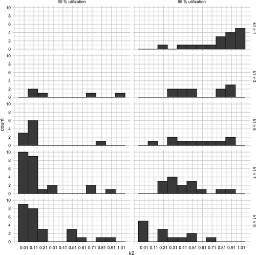
Considering the good performance of a tuned ATCS rule, favourable combinations of $k_1$ and $k_2$-values have been found using the parameter variation experiment. Based on 66 different product mixes and two utilisation levels, the number of occurrences of the best k-value combinations is plotted as a histogram in Figure 4. The two columns on the x-axis represent the 2 levels of utilisation (90% and 85%, respectively). On the x-axis of each sub-plot, the possible $k_2$-values are presented, ranging from 0.01 to 1.01 in steps of 0.1. The rows represent the different $k_1$-levels, ranging from 1 to 9, in a step size of 2. On the y-axis of each sub-plot the occurrence of the best $k_2$-value is given. Figure 4 proves that different product mixes at different utilisation levels are in need of individual k-values. Based on the number of occurrences, $k_1$ = 9 and $k_2$ = 0.11 for 90% and $k_1$ = 1 and $k_2$ = 0.91 for 85% utilisation are the best k-value combinations. Given these results, the combinations will lead to good performance for most of the product mixes and have a negative impact on a few others, depending on the utilisation level. To make this more obvious an example is given: assuming the $k_2$-value is set to 0.11, this will lead to good performance at high utilisation. Since only 6 product mixes use a $k_2$-value that small at 85% utilisation it will have a negative impact at the lower utilisation levels on most of the product mixes. This only applies, if all mixes are already known and used equally often.

Figure 4. Plotting the histogram of $k_2$-values leading to the best result in combination with the best $k_1$-value at different utilisations.

Multiple product mixes have been analysed further to show the behaviour in more detail. The second parameter variation experiment has been conducted with a finer grid for the planned utilisation level, as well as $k_1$-values. The range for the inter arrival times has been selected to catch the flip from large to small k-values for multiple product mixes. The intent of the study was to find the best product mix specific k-value combination at different levels of utilisation. Resulting k-values, for the mixes [70/30/0] to the left and [0/50/50] to the right, are shown in Table 2.

Table 2. Given the same planned utilisation ($Uti{l}_{pl}$) the best k-values for product mix [70/30/0] and [0/50/50] change as well as the resulting utilisation levels ($Uti{l}_{re}$).

$Uti{l}_{pl}$	$k_1$	$k_2$	$Uti{l}_{re}$	$k_1$	$k_2$	$Uti{l}_{re}$
	1	1.01	85.6%	1	0.61	87.6 %
	1	0.91	87.1%	2	0.51	88.9 %
85 %	1	0.61	88.4%	3	0.01	89.7 %
	2	0.61	89.9%	6	0.11	91.1 %
	6	0.51	91.3%	7	0.11	92.5 %
90 %	9	0.01	92.3%	8	0.11	93.8%

Given the previous references, the usage of neural networks or other regression methods to forecast the best k-values could be considered. A regression model would only be needed if the situation is unknown (e.g. unknown utilisation level). The values recorded during the second parameter variation study cover the important range of utilisation levels as well as a set of different product mixes and, therefore, have been used for a dynamic adjustment in the simulation. The observations provided as well as the time frame observed for the adjustments are similar with the one provided for the RL-agent. The values are referenced as ‘ Brute-Force’ in Figures 6 and 8.

5.3. Evaluation of the reinforcement learning approach

In the first part of the section, the used parameters and the training behaviour will be evaluated. Later the live performance of the agent will be shown and compared to the performance of the static application of the ATCS rule presented earlier.

The agent has been trained with the simulation model presented above. The simulation is terminated after 12,500 jobs have been processed, including the 2500 jobs warm up. Based on the temporal difference training method, different parameters for the agent have to be assessed. During the training the agent has to perform different actions and evaluate the impact on the performance. Provided the runtime of the simulation, different steps sizes lead to different amounts of (state,action)-pairs per episodes, for that the amount of actions per episode has to be considered. Two different time steps between consecutive actions have been tested: an action every day (1440 min) or every week (10,080 min). In this contribution, the step size of one week resulted in a more stable behaviour.

Further, the amount of episodes for the training need to be evaluated. Preliminary studies for this contribution showed, that the training of the agent for 200 episodes with 70 steps per episode each, led to feasible results for one product mix. During training with multiple product mixes, assuming that some (state, action)-pairs are similar for multiple product mixes, 1000 episodes, resulting in 70,000 steps, led to a stable policy for six product mixes. The number of actions taken could be increased up to one million, showing good results in other contributions (Stricker et al. 2018).

The mean tardiness was calculated for the 10,000 jobs processed after warm up. For that, the change between two steps, given one action, can hardly be measured. Especially in the later course of the simulation, actions did not affect the mean tardiness as much as choosing a bad parameter up front. To measure the performance more accurate, a new observation was introduced: the tardiness based on the last week in the system, representing about 200 jobs.

During each training step, 28 state parameters of the system are observed, e.g. the utilisation of all ten machines over the last week, their work in queue, the product mix, and the k-values used for sequencing. The mean tardiness of the last 10,000 jobs as well as the mean tardiness over the last week were recorded as key performance indicators for the system. The observations are summarised in Table 3. The action space can be described by the increase and decrease of $k_1$ by 1 limited by 1 and 10 and $k_2$ by 0.1, limited by 0.01 and 1.01.

Table 3. 28 observations are recorded during each state.

Observation in [unit]	Example
Average machine utilisation [%]	[90, 88, 92, 89, 97, 95, 91, 90, 91, 89]
Work in machine queue [min]	[50, 12, 18, 51, 89, 58, 39, 55, 21, 17]
Product mix [%]	[50, 50, 0, 0]
k-values	[7, 0.51]
short Tardiness [min]	210
mean Tardiness [min]	160

A short preliminary study showed that the usage of a fully connected neural network with 2 layers and 64 neurons each led to feasible results. Assuming that more product mixes during training represent a more complex system, a fully connected network with 2 layers and 300 neurons each, provided stable results as well. The amount of data points used for training of the neural network was set to 70, making sure that the neural network learned from each episode. The batch size of the neural network was set to 8.

The choice of how many steps used for the epsilon (ε) greedy annealing has a significant influence on the convergence behaviour and has been chosen so a convergence behaviour occurs within the last 15% of the training. The minimum ε-value has been set to 10% by default. The γ-value has been chosen to be 0.99 to ensure a positive long term strategy. The training of the agent resulted in a stable policy, for this reason its parameters have not been tuned further. The final training parameters are summarised in Table 4. Further analysis on the aspect of hyper parameter tuning need to be conducted later and are not part of this contribution.

Table 4. Parameters used to train the RL-agent in RL4J.

Parameter	Value
Steps per Epoch	70
Max. number of steps	70,000
Gamma	0.99
Minimum epsilon	0.1
Number steps for ε greedy	60,000

Multiple problems were encountered during the training, based on the reward function. Usually the total reward over one episode should converge towards an optimal value. When adjusting the k-values for the ATCS rule in small steps, the impact on the reward occasionally can hardly be measured and the reward doesn't improve significantly. Furthermore, increasing the s/p-ratio for product mixes resulted in increasing mean tardiness making them difficult to compare. Additionally, training on the various s/p-ratios, in need of different optimal k-values, made the convergence even more difficult.

Following, an RL-agent is presented, that adjusts the $k_1$ and $k_2$ values stepwise for the ATCS rule dynamically. In comparison to other machine learning approaches such as neural networks that only assign k-values, the actions of the RL-agent can be understood by humans as well.

The RL-approach was able to outperform the best static k-values [3, 0.01] and [1, 0.61] for the stable utilisation. Furthermore it was able to outperform the dynamic adjustment utilising the k-values recorded in the second parameter variation experiment for the product mixes presented earlier (reference Table 2). This can be explained by the inherent advantage, the dynamic adjustment, which plays to one's advantage. Since the optimal static k-values from the parameter variation are optimised based on the mean tardiness ignoring the variations within the simulation run, and for that, neglecting possible potential, the RL-agent is able to achieve lower mean tardiness. Given the information presented in the last paragraph of Section 5.2 and considering that the turn over effect of changing $k_2$ happens around 85% to 90% utilisation, choosing a good factor for a short amount of time, can reduce the mean tardiness. Since the agent is able to adjust the k-values during the execution of the simulation, based on the performance of the last week, he can choose actions that are beneficial for the system performance. For further illustration an example is given below. For the product mix [70/30/0], which has a low amount of setups, a large value of $k_2$ should lead to good results at 85% utilisation. As seen in Figure 5, the agent is able to reduce the $k_2$-value as the tardiness increases, and vice versa. The comparison of the static k-values and the RL-agent in a scenario with only one product mix can be seen in Figure 6.

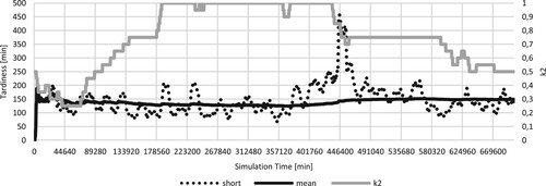
Figure 5. Fine adjustments to the $k_2$-value in a presumed static scenario can reduce the mean tardiness. The solid black line represents the mean tardiness in minutes over the last 10,000 jobs, the dotted line represents the mean tardiness in minutes over the last 200 jobs, both using the y-axis on the left. The grey line represents the $k_2$-value, using the axis on the right. On the x-axis the simulation time in minutes is presented.

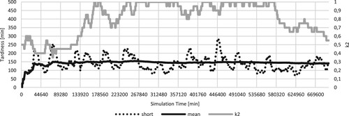
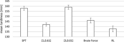
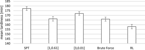
Figure 6. Comparing the different sequencing rules, it can be seen that the RL approach decreases mean tardiness by approximately 5% compared to the best static k-values found before.

This effect can also be seen if the product mix changes. For further demonstration of the effect, two opposing product mixes are considered in the next experiment ([70/30/0] and [0/50/50]). Assuming that the first product mix runs for about 3/4 of a year, the product mix has to change for 1/4 of a year and then back again, the prior known k-values might no longer be suitable. In Figure 7, it can be seen that the agent lowers the $k_2$-value to compensate the rise in mean tardiness. Reaching 3/4 of a year (around 400,000 min) a positive trend can be recognised in the short and the mean tardiness, resulting from the change in product mix and increased utilisation. Three months later (144,000 min), the short tardiness drops and levels again, due to the product mix changing back, resulting in a slight decrease in the $k_2$-value.

Figure 7. Adjusting the $k_2$-value to the new state of the system can reduce the mean tardiness significantly. The solid black line represents the mean tardiness in minutes over the last 10,000 jobs, the dotted line represents the mean tardiness in minutes over the last 200 jobs, both using the y-axis on the left. The grey line represents the $k_2$-value, using the axis on the right. On the x-axis the simulation time in minutes is presented.

The agent's actions can be explained using the knowledge about $k_2$, presented earlier. Since the first product mix has a low amount of setups a large value for $k_2$ should be considered for the utilisation of 85%. The same large $k_2$-value will result in massive delays with the second product mix, which has notably more setups and a higher utilisation. Choosing a small value for $k_2$ to account for that rare case will lead to an increase in mean tardiness for the first product mix. This motivates the dynamic adjustment of the k-values and proves that the agent adjusts the $k_2$-values plausible.

The results of the experiment with the changing product mix during the runtime are presented in Figure 8. The two sets of static k-values for each product mix are considered and compared to the single attribute sequencing rule. Providing the reference value for SPT, these can reduce the mean tardiness by up to 10%. Still. these static values are beaten by the RL approach by another 5%. This shows that the agent trained with RL can automatically transfer and apply the knowledge learned during the training to different and complex scenarios.

Figure 8. Considering the change of a product mix during the production both sets of k-values provide a stable mean which can be reduced by the RL-agent by approximately 5%.

To prove the stability of the approach, the scenarios have been replicated 30 times and it can be seen that the mean tardiness can be reduced significantly, up to 5% on either cases. In the first case, shown in Figure 6, the RL approach is able to reduce the mean tardiness compared to the best single attribute priority sequencing rule and slightly compared to the best k-values found by the extensive simulation study. In the second case, the agent was able to transfer knowledge and reduce the mean tardiness significantly in an unknown scenario. Both cases prove that the usage of an RL-agent to adjust the k-values for the ATCS rule can reduce the mean tardiness up to 5% compensating fluctuation within the system, introduced by internal and external stimuli.

6. Outlook and conclusion

In this paper, a flexible flow shop environment with sequence-dependent setup times and transportation time has been analysed regarding the usage of RL to train an agent to dynamically adjust the k-values for an ATCS rule. For the comparison a benchmark was established, based on a parameter variation experiment with a discrete event simulation model. During the evaluation, it became obvious that single attribute sequencing rules are outperformed by more complex rules, so-called composite rules. Using the state-of-the-art ATCS rule, the k-values have been optimised for various combinations of product mixes and system states. An RL-agent has been trained to dynamically adjust the k-values based on product mix and system utilisation, using the same discrete event simulation. Its behaviour has been analysed and it is shown that the trained agent can be used to adjust k-values dynamically and reduce the mean tardiness up to 5% in various scenarios.

Further evaluation of the approaches should include the aspects of routing products and dispatching vehicles if the transportation time increases. Additionally, the response to unplanned interruptions such as machine break down or priority jobs can be considered. Given the fact that ATCS as sequencing rule has been beaten by more complex composite rules, generated with genetic programming, the RL approach has to be tested against these approaches as well. Given the much larger and more complex solution space, the combination of an agent trained with RL and adjusting weights in a composite rule, has to be evaluated. In the future, the interaction effect of the individual factors within the rules could be evaluated in more detail.

Disclosure statement

No potential conflict of interest was reported by the author(s).

Additional information

Notes on contributors

Jens Heger

Jens Heger is a Professor at Leuphana University in Lueneburg. He has been leading the work group ‘modeling and simulation of technical systems and processes’ at the Institute of Product and Process Innovation. Furthermore, he is a speaker at the research centre for digital transformation at Leuphana University. During his doctorate in the field of production engineering, he worked on various research projects as a Research Associate. Since 2015, he has been a Junior Professor at Leuphana University in Lueneburg. His research focuses on the dynamic adjustment of parameters based on system states. He is leading various projects with different funding agencies. His e-mail address is [email protected]

Thomas Voss

Thomas Voss is a Research Associate at Leuphana University. He completed his studies as an industrial engineer with a focus on production engineering in 2016. He graduated with a master thesis on the optimal scheduling of autonomous guided vehicles in a blocking job shop environment. His Ph.D. project is a follow up on this topic and includes the sequencing and routing of operations in a manufacturing system. He has been able to gain experience in simulation and optimisation through various projects. His e-mail address is [email protected].

References

- Adams, Joseph, Egon Balas, and Daniel Zawack. 1988. “The Shifting Bottleneck Procedure for Job Shop Scheduling.” Management Science 34 (3): 391–401. http://www.jstor.org/stable/2632051 doi: 10.1287/mnsc.34.3.391
- Baker, Kenneth R 1984. “The Effects of Input Control in a Simple Scheduling Model.” Journal of Operations Management 4 (2): 99–112. doi: 10.1016/0272-6963(84)90026-3
- Branke, Jürgen, Torsten Hildebrandt, and Bernd Scholz-Reiter. 2015. “Hyper-Heuristic Evolution of Dispatching Rules: A Comparison of Rule Representations.” Evolutionary Computation 23 (2): 249–277. doi: 10.1162/EVCO_a_00131
- Branke, Jurgen, Su Nguyen, Christoph W. Pickardt, and Mengjie Zhang. 2016. “Automated Design of Production Scheduling Heuristics: A Review.” IEEE Transactions on Evolutionary Computation 20 (1): 110–124. doi: 10.1109/TEVC.2015.2429314
- Chen, Jenny Yan, Michele E. Pfund, John W. Fowler, Douglas C. Montgomery, and Thomas E. Callarman. 2010. “Robust Scaling Parameters for Composite Dispatching Rules.” IIE Transactions 42 (11): 842–853. doi: 10.1080/07408171003685825
- Chen, Shengkai, Shuiliang Fang, and Renzhong Tang. 2019. “A Reinforcement Learning Based Approach for Multi-projects Scheduling in Cloud Manufacturing.” International Journal of Production Research 57 (10): 3080–3098. doi: 10.1080/00207543.2018.1535205
- Chen, Yan 2013. “Loss Function Based Robust Scaling Parameters for Composite Dispatching Rule ATCS.” In 2013 International Conference on Engineering, Management Science and Innovation (ICEMSI), Macao, China, 1–3. IEEE.
- Fazlollahtabar, Hamed, Mohammad Saidi-Mehrabad, and Ellips Masehian. 2015. “Mathematical Model for Deadlock Resolution in Multiple AGV Scheduling and Routing Network: A Case Study.” Industrial Robot: An International Journal 42 (3): 252–263. doi: 10.1108/IR-12-2014-0437
- Gabel, Thomas. 2009. “Multi-agent Reinforcement Learning Approaches for Distributed Job-Shop Scheduling Problems.” PhD diss., Universität Osnabrück, Osnabrück.
- Gabel, Thomas, and Martin Riedmiller. 2008. “Adaptive Reactive Job-shop Scheduling with Reinforcement Learning Agents.” International Journal of Information Technology and Intelligent Computing 24 (4): 14–18.
- Gallay, Olivier, Kari Korpela, Niemi Tapio, and Jukka K. Nurminen. 2017. “A Peer-to-peer Platform for Decentralized Logistics.” In Proceedings of the Hamburg International Conference of Logistics (HICL), Hamburg, Germany, 19–34. epubli. doi:10.15480/882.1473.
- Graham, Ronald L., Eugene L. Lawler, Jan Karel Lenstra, A. Rinnooy, and H. G. Kan. 1979. “Optimization and Approximation in Deterministic Sequencing and Scheduling: A Survey.” Annals of Discrete Mathematics 5: 287–326. doi: 10.1016/S0167-5060(08)70356-X
- Heger, Jens. 2014. Dynamische Regelselektion in Der Reihenfolgeplanung. Wiesbaden: Springer Fachmedien Wiesbaden.
- Heger, Jens, Jürgen Branke, Torsten Hildebrandt, and Bernd Scholz-Reiter. 2016. “Dynamic Adjustment of Dispatching Rule Parameters in Flow Shops with Sequence-Dependent Set-up Times.” International Journal of Production Research 54 (22): 6812–6824. doi: 10.1080/00207543.2016.1178406
- Heger, Jens, and Thomas Voß. 2020. “Dynamically Changing Sequencing Rules with Reinforcement Learning in a Job Shop System with Stochastic Influences.” In Proceedings of the Winter Simulation Conference, edited by K.-H. Bae, B. Feng, S. Kim, S. Lazarova-Molnar, Z. Zheng, T. Roeder, and R. Thiesing, 1608–1618. Orlando, FL: IEEE. doi:10.1109/WSC48552.2020.9383903.
- Holland, John H. 1984. “Genetic Algorithms and Adaptation.” In Adaptive Control of Ill-Defined Systems, edited by Oliver G. Selfridge, Edwina L. Rissland, and Michael A. Arbib, 317–333. Boston, MA: Springer US.
- Jun, Sungbum, and Seokcheon Lee. 2021. “Learning Dispatching Rules for Single Machine Scheduling with Dynamic Arrivals Based on Decision Trees and Feature Construction.” International Journal of Production Research 59 (9): 2838–2856. doi: 10.1080/00207543.2020.1741716
- Kardos, Csaba, Catherine Laflamme, Viola Gallina, and Wilfried Sihn. 2021. “Dynamic Scheduling in a Job-shop Production System with Reinforcement Learning.” Procedia CIRP 97: 104–109. doi: 10.1016/j.procir.2020.05.210
- Knust, Sigrid. 1999. Shop scheduling problems with transportation: Diss. Osnabrück: Universität Osnabrück, Fachbereich Mathematik/Informatik.
- Kuhnle, Andreas. 2020. Adaptive Order Dispatching Based on Reinforcement Learning: Application in a Complex Job Shop in the Semiconductor Industry. Vol. Band 241 of Forschungsberichte aus dem wbk, Institut für Produktionstechnik, Karlsruher Institut für Technologie (KIT). Düren: Shaker Verlag GmbH.
- Kuhnle, Andreas, Jan-Philipp Kaiser, Felix Theiß, Nicole Stricker, and Gisela Lanza. 2020. “Designing An Adaptive Production Control System Using Reinforcement Learning.” Journal of Intelligent Manufacturing 32: 855–876. doi: 10.1007/s10845-020-01612-y
- Kuhnle, Andreas, Nicole Röhrig, and Gisela Lanza. 2019. “Autonomous Order Dispatching in the Semiconductor Industry Using Reinforcement Learning.” Procedia CIRP 79: 391–396. doi: 10.1016/j.procir.2019.02.101
- Kumar, Rajeev. 2016. “Simulation of Manufacturing System at Different Part Mix Ratio and Routing Flexibility.” Global Journal of Enterprise Information System 8 (1): 10–14. doi: 10.18311/gjeis/2016/7284
- Lee, Young Hoon, Kumar Bhaskaran, and Michael Pinedo. 1997. “A Heuristic to Minimize the Total Weighted Tardiness with Sequence-dependent Setups.” IIE Transactions 29 (1): 45–52. doi: 10.1080/07408179708966311
- May, Marvin Carl, Lars Kiefer, Andreas Kuhnle, Nicole Stricker, and Gisela Lanza. 2021. “Decentralized Multi-Agent Production Control Through Economic Model Bidding for Matrix Production Systems.” Procedia CIRP 96: 3–8. doi: 10.1016/j.procir.2021.01.043
- Mnih, Volodymyr, Koray Kavukcuoglu, David Silver, Andrei A. Rusu, Joel Veness, Marc G. Bellemare, Alex Graves, et al., 2015. “Human-level Control Through Deep Reinforcement Learning.” Nature 518 (7540): 529. doi: 10.1038/nature14236
- Mönch, Lars, Jens Zimmermann, and Peter Otto. 2006. “Machine Learning Techniques for Scheduling Jobs with Incompatible Families and Unequal Ready Times on Parallel Batch Machines.” Engineering Applications of Artificial Intelligence 19 (3): 235–245. doi: 10.1016/j.engappai.2005.10.001
- Nguyen, Su, Yi Mei, and Mengjie Zhang. 2017. “Genetic Programming for Production Scheduling: a Survey with a Unified Framework.” Complex & Intelligent Systems 3 (1): 41–66. doi: 10.1007/s40747-017-0036-x
- Oukil, Amar, and Ahmed El-Bouri. 2021. “Ranking Dispatching Rules in Multi-objective Dynamic Flow Shop Scheduling: a Multi-faceted Perspective.” International Journal of Production Research 59 (2): 388–411. doi: 10.1080/00207543.2019.1696487
- Panwalkar, S. S., and Wafik Iskander. 1977. “A Survey of Scheduling Rules.” Operations Research 25 (1): 45–61. http://www.jstor.org/stable/169546 doi: 10.1287/opre.25.1.45
- Park, Youngshin, Sooyoung Kim, and Young-Hoon Lee. 2000. “Scheduling Jobs on Parallel Machines Applying Neural Network and Heuristic Rules.” Computers & Industrial Engineering 38 (1): 189–202. doi: 10.1016/S0360-8352(00)00038-3
- Pickardt, Christoph W., Torsten Hildebrandt, Jürgen Branke, Jens Heger, and Bernd Scholz-Reiter. 2013. “Evolutionary Generation of Dispatching Rule Sets for Complex Dynamic Scheduling Problems.” International Journal of Production Economics 145 (1): 67–77. doi: 10.1016/j.ijpe.2012.10.016
- Poppenborg, Jens, Sigrid Knust, and Joachim Hertzberg. 2012. “Online Scheduling of Flexible Job-shops with Blocking and Transportation.” European Journal of Industrial Engineering (EJIE) 6 (4): 497–518. doi: 10.1504/EJIE.2012.047662
- Qu, T., S. P. Lei, Z. Z. Wang, D. X. Nie, X. Chen, and George Q. Huang. 2016. “IoT-based Real-time Production Logistics Synchronization System Under Smart Cloud Manufacturing.” The International Journal of Advanced Manufacturing Technology 84 (1-4): 147–164. doi: 10.1007/s00170-015-7220-1
- Riley, Michael, Yi Mei, and Mengjie Zhang. 2016. “Improving Job Shop Dispatching Rules Via Terminal Weighting and Adaptive Mutation in Genetic Programming.” In 2016 IEEE Congress on Evolutionary Computation (CEC), 3362–3369. Piscataway, NJ: Institute of Electrical and Electronics Engineers.
- Scholz-Reiter, Bernd, Jens Heger, Christian Meinecke, and Johann Bergmann. 2010. “Materialklassifizierung Unter Einbeziehung Von Bedarfsprognosen.” Productivity Management 15 (1): 57–60. http://fox.leuphana.de/portal/de/publications/materialklassifizierung-unter-einbeziehung-von-bedarfsprognosen(61e557ff-32c6-4f9e-9731-45e91103203b).html
- Sharma, Pankaj, and Ajai Jain. 2016. “Effect of Routing Flexibility and Sequencing Rules on Performance of Stochastic Flexible Job Shop Manufacturing System with Setup Times: Simulation Approach.” Proceedings of the Institution of Mechanical Engineers, Part B: Journal of Engineering Manufacture 231 (2): 329–345. doi: 10.1177/0954405415576060
- Shi, Lei, Gang Guo, and Xiaohui Song. 2021. “Multi-Agent Based Dynamic Scheduling Optimisation of the Sustainable Hybrid Flow Shop in a Ubiquitous Environment.” International Journal of Production Research 59 (2): 576–597. doi: 10.1080/00207543.2019.1699671
- Shiue, Yeou-Ren, Ken-Chuan Lee, and Chao-Ton Su. 2018. “Real-time Scheduling for a Smart Factory Using a Reinforcement Learning Approach.” Computers & Industrial Engineering 125: 604–614. doi: 10.1016/j.cie.2018.03.039
- Shiue, Yeou-Ren, Ken-Chuan Lee, and Chao-Ton Su. 2020. “A Reinforcement Learning Approach to Dynamic Scheduling in a Product-Mix Flexibility Environment.” IEEE Access 8: 106542–106553. doi: 10.1109/ACCESS.2020.3000781
- Silver, David, Julian Schrittwieser, Karen Simonyan, Ioannis Antonoglou, Aja Huang, Arthur Guez, Thomas Hubert, et al., 2017. “Mastering the Game of Go Without Human Knowledge.” Nature 550 (7676): 354. doi: 10.1038/nature24270
- Stricker, Nicole, Andreas Kuhnle, Roland Sturm, and Simon Friess. 2018. “Reinforcement Learning for Adaptive Order Dispatching in the Semiconductor Industry.” CIRP Annals 67 (1): 511–514. doi: 10.1016/j.cirp.2018.04.041
- Vepsalainen, Ari P. J., and Thomas E. Morton. 1987. “Priority Rules for Job Shops with Weighted Tardiness Costs.” Management Science 33 (8): 1035–1047. doi: 10.1287/mnsc.33.8.1035
- Vinyals, Oriol, Timo Ewalds, Sergey Bartunov, Petko Georgiev, Alexander Sasha Vezhnevets, Michelle Yeo, Alireza Makhzani, and et al. 2017. “Starcraft II: A New Challenge for Reinforcement Learning.” preprint arXiv:1708.04782.
- Waschneck, Bernd, André Reichstaller, Lenz Belzner, Thomas Altenmüller, Thomas Bauernhansl, Alexander Knapp, and Andreas Kyek. 2018. “Optimization of Global Production Scheduling with Deep Reinforcement Learning.” Procedia CIRP 72 (1): 1264–1269. doi: 10.1016/j.procir.2018.03.212
- Wuest, Thorsten, Daniel Weimer, Christopher Irgens, and Klaus-Dieter Thoben. 2016. “Machine Learning in Manufacturing: Advantages, Challenges, and Applications.” Production & Manufacturing Research 4 (1): 23–45. doi: 10.1080/21693277.2016.1192517
- Zhang, Fangfang, Yi Mei, Su Nguyen, and Mengjie Zhang. 2020. “Genetic Programming with Adaptive Search Based on the Frequency of Features for Dynamic Flexible Job Shop Scheduling.” In Evolutionary Computation in Combinatorial Optimization, edited by Luís Paquete and Christine Zarges, Vol. 12102 of Lecture Notes in Computer Science, 214–230. Cham: Springer International Publishing.
- Zhang, Fangfang, Yi Mei, and Mengjie Zhang. 2018. “Genetic Programming with Multi-tree Representation for Dynamic Flexible Job Shop Scheduling.” In AI 2018, edited by Tanja. Mitrovic, Bing. Xue, and Xiaodong. Li, Vol. 11320 of LNCS sublibrary. SL 7, Artificial intelligence, 472–484. Cham: Springer.
- Zhang, Fangfang, Yi Mei, and Mengjie Zhang. 2019. “Can Stochastic Dispatching Rules Evolved by Genetic Programming Hyper-heuristics Help in Dynamic Flexible Job Shop Scheduling?” In 2019 IEEE Congress on Evolutionary Computation (CEC), Wellington, New Zealand, 41–48. IEEE. doi:10.1109/CEC.2019.8790030.
- Zhang, Fangfang, Yi Mei, and Mengjie Zhang. 2019. “A Two-Stage Genetic Programming Hyper-Heuristic Approach with Feature Selection for Dynamic Flexible Job Shop Scheduling.” In GECCO 2019: Proceedings of the Genetic and Evolutionary Computation Conference, 347–355. New York, NY: Association for Computing Machinery. doi:10.1145/3321707.3321790.
- Zhao, Meng, Xinyu Li Liang Gao, Ling Wang, and Mi Xiao. 2019. “An improved Q-Learning Based Rescheduling Method for Flexible Job-Shops with Machine Failures.” In 2019 IEEE 15th International Conference on Automation Science and Engineering (CASE), 331–337. Piscataway, NJ: Institute of Electrical and Electronics Engineers.
- Zheng, Shuai, Chetan Gupta, and Susumu Serita. 2019. “Manufacturing Dispatching Using Reinforcement and Transfer Learning.” preprint arXiv:1910.02035.