Visualisation of ripple effect in supply chains under long-term, simultaneous disruptions: a system dynamics approach

Abstract

Supply chains (SCs) are exposed to multiple risks and vulnerable to disruption propagation (i.e. the ripple effect). Despite established literature, quantitative analysis of the ripple effect in SCs considering simultaneous, long-term disruptions (i.e. induced by the COVID-19 pandemic) remains limited. This study defines, applies and demonstrates the capability of system dynamics modelling to recognise and visualise the ripple effect subject to supply, demand, and logistics disruptions as well as a combined, simultaneous disruption of supply, demand and logistics. Simulation results for these four risk scenarios indicate that disruption propagation and its impacts vary based on risk type, combination of risks and the impacting node. The bi-directional, increasing effect is significant for disruptions of longer duration. Retailers and manufacturers are most fragile to multiple disruptions due to broader risk exposure points. In generalised terms, systems theory-based study provides insights into the complex behaviour of simultaneous risks and associated disruptions occurring at a node and across the SC. The outcomes derived can help practitioners visualise and recognise the dynamic nature of the ripple effect cascading across the SC network. In addition, some novel insights on the systemic nature and delayed impact of disruption propagations are uncovered and discussed.

KEYWORDS:

• Supply chain risk management
• ripple effect
• risk propagation
• disruption propagation
• risk modelling
• system dynamics

1. Introduction

Supply chains (SCs) are exposed to different risks, including operational, environmental and human-made risks (Rao and Goldsby 2009; Ho et al. 2015). The disruptions caused by different risks adversely affect the SC network (Heckmann, Comes, and Nickel 2015). One difficulty in managing SC disruption is that they cascade through a wider network, causing a ripple effect, devastating an organisation's financial and operational performance (Dolgui, Ivanov, and Sokolov 2018; Hosseini and Ivanov 2020). The ‘ripple effect’ also called ‘risk/disruption propagation’ is defined as cascading impact of a risk disrupting not just a single SC node but further propagating across the supply, production and distribution nodes in SC network (Ghadge, Dani, and Kalawsky 2012; Ivanov, Sokolov, and Dolgui 2014).

Despite the remarkable progress in the ripple effect research (Dolgui and Ivanov 2021), little is known about disruption propagation under long-term disruptions when demand, supply and logistics are disrupted sequentially and simultaneously at different SC echelons. For some years, such scenarios have been considered rather unlikely. However, the example of COVID-19 pandemic demonstrates such environments highlighting the scope and scale of the disruption propagation across the global SC network (Paul and Chowdhury 2020; El Baz and Ruel 2021; Nagurney 2021; Sodhi, Tang, and Willenson 2021). In early 2020, Haren and Simch-Levi (2020) observed a ripple effect immediately after the COVID-19 epidemic outbreak in China at Fiat Chrysler Automobiles and Hyundai. Over the same year, the ripple effect scale grew substantially, adversely affecting almost all the industries and services worldwide (Singh et al. 2020; Ruel et al. 2021). Due to the global nature of disruption over a relatively long period, it provides an excellent opportunity to study independent and simultaneous risks over a long-term horizon.

SC literature on the ripple effect focuses on conceptualising (Dolgui, Ivanov, and Sokolov 2018) or establishing the impact of risk type on a specific SC node (Kinra et al. 2020). Episodically, studies attempt to quantify the ripple effect of risk on SC network (e.g. Sokolov et al. 2016; Ojha et al. 2018); however, there is a lack of understanding of the cascading disruptive effects of simultaneous (combination of) risks on different SC nodes (Llaguno, Mula, and Campuzano-Bolarin 2021). This is critical for today’s global SCs, as they are faced with multiple, simultaneous risks to their daily operations repeatedly. The combined disruptive impact of these risks is difficult to predict and visualise holistically due to the inherent complexity and interconnectedness of different SCs and risk variables. Thus, this study attempts to model and capture the impact of disruption propagation of both individual and multiple simultaneous risks on different SC nodes. To this end, the study aims to visualise the ripple effect in SCs characterised by severe disruptions due to demand, supply and logistics risk, which may happen sequentially or simultaneously in the case of pandemic-like crises.

An integrative perspective is essential for modelling disruption propagation across the SC networks; however, most current models are dominated by optimisation approaches (Dolgui, Ivanov, and Sokolov 2018), while lacking visualised models to imitate (simulate) different scenarios to assess the disruption propagation phenomenon from a multifaceted and micro perspective (Pavlov et al. 2019; Llaguno, Mula, and Campuzano-Bolarin 2021). Thus, following system dynamics (SD) approach, this study develops and tests a simulation model to capture the impact of long-term, simultaneous disruptions. Four disruptions scenarios are induced by demand, supply and logistics risk independently and simultaneously to address the evident research gap. Secondary data made available by a leading aerospace and defence company based in the UK was used for the study. The data comprised multiple human-made, and natural SC risks the company faced within their global business operations over the last five years.

The remainder of the paper is structured as follows. Section 2 provides a brief background of the ripple effect in SCs. Section 3 summarises the research methodology and Section 4 presents the proposed SD model. Section 5 discusses the results of simulation modelling. In Section 6, the key findings are discussed and related to novel theoretical and managerial implications. The concluding Section 7 summarises our study's key results and outlines its limitations and future research opportunities.

2. Background

The research interest on the ripple effect has grown significantly over the past decade due to increased risk events and awareness within academia and industry. The term ‘ripple effect’ refers to disruption propagation from a node to other parts of the SC network (Dolgui, Ivanov, and Sokolov 2018; Chauhan, Perera, and Brintrup 2021; Gholami-Zanjani et al. 2021). Once a disruption occurs at one specific node, the whole SC may be impacted due to SC functions’ interconnectivity and interdependency (Deng et al. 2019; Goldbeck, Angeloudis, and Ochieng 2020). Several other terminologies are interchangeably used for a ripple effect in the SC literature, namely ‘risk diffusion’ (Basole and Bellamy 2014), ‘snowball or domino effect’ (Swierczek 2016) and ‘cascading effect’ (Heckmann, Comes, and Nickel 2015) to name a few. This phenomenon has also been referred to as ‘risk propagation’ (Ghadge, Dani, and Kalawsky 2012; Ojha et al. 2018; Li et al. 2020) or ‘disruption propagation’ (Wu, Blackhurst, and O’Grady 2007; Bueno-Solano and Cedillo-Campos 2014; Scheibe and Blackhurst 2018; Ivanov and Dolgui 2020). Despite different terminologies existing in SC literature, the fundamental concept remains the same.

Conceptualising, modelling and capturing disruption propagation impact is critical for understanding SC network vulnerability and building resilient SC structures (Ghadge et al. 2013). However, a limited amount of research specifies the ripple effect caused by disruptions with low frequency and high impact (such as supplier unavailability, transport disruption and production disruption) (Dolgui, Ivanov, and Sokolov 2018). Specific research attempting to quantify the ripple effect considering singular and combined disruptions in demand, capacity and supply dynamics is not found in the extant literature.

Similar insights generated through modelling of disruption propagation are being utilised for improving SC performance and resilience. However, few studies demonstrate that simulation models can help analyse multi-echelon SCs’ behaviour with multiple and long-term risks to understand disruption propagation triggers and mechanisms (Wilson 2007; Macdonald et al. 2018; Llaguno, Mula, and Campuzano-Bolarin 2021). Existing simulation models usually capture a limited number of SC nodes and time intervals (Bueno-Solano and Cedillo-Campos 2014; Kinra et al. 2020). The significant advantage of SD comes from its ability to visualise and quantify intricate and dynamic systems by capturing causal relationships between different variables, risk factors and their consequential behaviours (Wilson 2007). Compared with other mathematical models, which require sophisticated algorithms and structures with various limitations, it has been acknowledged in previous studies that the SD model can address the non-linear and linear behaviours of a complex system in a realistic, relatively simplified manner (Er Kara, Ghadge, and Bititci 2020). Furthermore, SD enables different scenario-based sensitivity analysis. Sensitivity analysis helps assess and interpret the potential consequences of risk propagation under different risk scenarios to provide deeper insights and make informed decisions.

Despite the broad application of simulation for modelling the ripple effect in SCs, little is known about its potential to visualise and recognise the ripple effect's dynamic nature under such multiple and simultaneous risks. Studying global disasters such as the COVID-19 pandemic (2020) helps holistically assess disruption propagation across the entire SC network (Ivanov 2020). Our study aims to close this research gap.

3. Research methodology

In this study, we model disruption propagation within a four-echelon SC faced with multiple (independent and simultaneous) risks. For modelling such a phenomenon, we consider multiple SC risks and associated variables interacting with each other. These interactions result in complexity due to the interdependence of many factors/variables and multiple feedback loops (Mingers and White 2010). For assessing such complex interactions, systems thinking/dynamics is the most suitable approach (Foerster 1968; Sterman 2010). Furthermore, systems thinking helps build an SD model to simulate interconnected environments (Kamath and Roy 2007; Mula et al. 2013). Past research shows that SD simulation is a powerful technique to model complexity, multidimensionality and interrelations of a real-world SC system (e.g. Ghadge et al. 2013; Ivanov 2017; Scheibe and Blackhurst 2018; Er Kara, Ghadge, and Bititci 2020; Rathore, Thakkar, and Jha 2020).

For SC risk assessment, different simulation modelling approaches have been utilised to capture credible representations of real systems. Apart from SD modelling, agent-based modelling (ABM), discrete event simulation (DES), Monte-Carlo simulation are commonly used for modelling real systems (Janssen, Sharpanskykh, and Curran 2019; Rathore, Thakkar, and Jha 2020). Each of these methods has its advantages and disadvantages. ABM simulates actions and interactions of autonomous decision-making entities (agents) that act according to their own goals (Nilsson and Darley 2006). While SD modelling focuses on the flows, feedbacks and cumulative longitudinal effects (Foerster 1968), and ABM considers the spatial interactions rather than feedback effects of the factors (Ding et al. 2018). DES models a series of discrete events and considers networks of queues. While DES models are stochastic and focus more on numerical results, SD models generally show deterministic behaviour and focus on the events that lead to changes in the system (Tako and Robinson 2009).

The SD approach was found to be appropriate to model dynamic SC systems for apprehending disruption propagation within SC nodes. The global impact of the COVID-19 pandemic has shown the importance of building simulation-based systems for disruption mapping and risk modelling (Choi, Rogers, and Vakil 2020; Currie et al. 2020; Ivanov and Dolgui 2020). Such simulation models help companies develop proactive risk management frameworks and identify efficient recovery policies.

The research design in this study is as follows. First, the key variables and interrelationships within the SC system were defined. Then, the causal loop and stock and flow diagram were developed. These diagrams provide a rough representation of a system to capture the dynamics of different influential variables. The accuracy of these diagrams is confirmed by validating whether the interventions have the desired impact. Later, the model was simulated for different scenarios to draw inferences. Finally, a classical four-echelon SC model, including supplier, manufacturer, distributor and retailer, was considered to analyse the propagation of risks along the entire SC.

To develop a causal loop diagram (CLD), causalities of variables and parameters were depicted. The CLD was then converted into a stock and flow diagram, which allows quantitative analysis of the system using SD computer software-Vensim PLE^®. For simulation purposes, supplier capacity, transport capacity and market demand were assumed to be exposed to varying risks. Variations in different SC variables were examined to understand the impact of such risks and their disruption propagation along the SC. These variations were captured by measuring the ‘vulnerability index’ at each time interval for SC nodes.

Different conditions were simulated by changing input risk parameters for two severity levels; moderate and high disruption cases. The risk scenarios comprise demand risk, logistics risk, supply risk and multiple parallel risks during a specific time interval. Parametric values utilised in the simulation model were based on the secondary data of a leading aerospace and defence company based in the UK. This data set provides the researcher with more in-depth insights about SC under different risks/disruptions at different locations/nodes and their relative impact in the broader aerospace industry.

4. Model development

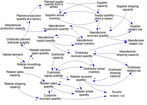
To build the SD model, key SC variables and influential risk factors were identified based on the literature review and authors’ experience within SCRM. Typically, there may be numerous risk factors related to each SC entity interacting with the entire system, constituting an accumulated vulnerability exposure. Key risks considered in the model refer to supply, logistics and demand risk. Actual inventory levels of the supplier, manufacturer and distributor, shipping capacity of the manufacturer and market demand were considered for capturing the disruption effect. Figure 1 shows the CLD of the model developed following the identification of the key SC variables, risk factors and feedback loops between variables revealing the cascading phenomenon. The following steps were applied to capture a holistic as well as reliable model; (i) the model was refined iteratively by exploring the usefulness of the model via multiple discussions with industry experts and authors. Here, we utilised production and SC professionals and authors expertise in SCRM for refinement of the CLD model. (ii) Multiple settings were tried to capture different scenarios based on the real working environment of the practitioners. Finally, the CLD was developed by selecting multiple variables, flows and interrelationships.

Figure 1. Causal loop diagram.

The accuracy of developed CLD was validated by performing several tests (refer to Appendix 2) to check whether the interventions have the desired impact.

The CLD demonstrates the numerical variations of multiple influential variables. The direction of one variable to another is represented with ‘+’ and ‘−’ signs in the CLD. For example, supplier capacity positively impacts the supplier's actual inventory, i.e. an increase in supplier capacity can improve a supplier's actual inventory (Lücker, Chopra, and Seifert 2020). As observed in Figure 1, four negative feedback loops exist in this system, comprising relationships between output quantity and actual inventory level at each SC entity. Since the number of loops is even, this SC system is recognised to be stable.

Variations and discrepancies in SC variables were captured as vulnerabilities, disrupting the SC system. For example, the difference between a supply quantity from a vendor and the actual quantity received at a manufacturer represents a supplier-related risk inducing inventory risk or transport risk in the model. Identification of other SC entity-related risks follows the same rationale mentioned above. Differences between manufacturer-received quantity from supplier and distributor and actual received quantity present the manufacturer-related risk, including inventory, transport and production-related risks. Apart from key variables, the CLD also considers several relevant auxiliary variables such as planned quantity and shipping capacity at each node of the SC, which connects every node and constitutes the holistic SC system.

To simplify the model and run the simulation, the following assumptions were made:

• The causes of variations and discrepancies among the variables only consider major risk, i.e. inventory and transport risk at every SC node.

• The expected inventory level, initial inventory level, capacity and transport capacity at each SC node is based on the secondary data.

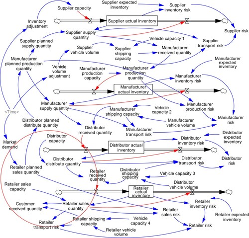
Figure 2 shows the stock and flow diagram developed from the CLD by carefully filtering key influential (direct and indirect) variables into ‘stocks’ and ‘flows’. The stock and flow diagram was then fed with the input data (initial value, rate of flows, etc.). This SD model was tested for relevance, consistency, sensitivity and extreme condition test (Martis 2006). The model was found to be feasible and valid for the intended purpose of capturing disruption propagation. The proposed SD model was simulated for 156 weeks, and the SC was exposed to demand, transportation and supply risks within 72–110 weeks to analyse disruption propagation across the SC. Numerical settings and main equations of the SD model may be found in Appendix 1.

Figure 2. Stock and flow diagram.

5. Simulation results

The developed simulation model was run using the Vensim PLE platform. Each scenario-based simulation was run once, each run comprising of minimum 200 iterations before obtaining results. Supplier risk was calculated based on inventory and transportation risk variables identified at the supplier node available in the secondary data. Similarly, manufacturer risk was measured based on a manufacturer’s inventory, production and transportation risk. The specific risk exposure level at distributor and retailer nodes showed a relatively stable level within the available data. Four different risk scenarios were designed by considering selected risks (market demand, transport capacity shortages, supply-related issues) occurring at each SC node to understand the degree of vulnerability of each SC node due to cascading impact of disruption propagation. According to Svensson (2002a, p. 65), ‘vulnerability is a condition that is caused by time and relationship dependencies in a company’s business activities in supply chains. The degree of vulnerability may be interpreted as proportional to the degree of time and relationship dependencies, and the negative consequence of these dependencies, in a company’s business activities towards suppliers and customers’. According to the above definition, the construct of vulnerability consists of two components: disturbance and the negative consequence of disturbance. A disturbance is a random deviation from what is normal or expected. A negative consequence of disturbance refers to a deteriorated goal accomplishment in terms of economic costs, increased cycle times and downtimes (Svensson 2002b). Adopting this concept of ‘vulnerability’ in the study, we attempt to depict variation in vulnerability at each SC node due to impacting risk and their cascading disruption to other SC nodes over a selected time horizon. This variation in vulnerability is calculated using the ‘vulnerability index’ (adopted from Wagner and Neshat 2010) and varied between 0 and 1. The vulnerability index is a numerical value that measures exposure to risks/hazards and is calculated by combining quantitative weighted risk scores to get a cumulative value. Vulnerability logic diagrams and event trees are frequently used to estimate vulnerability accurately (Janssen, Sharpanskykh, and Curran 2019). Under normal operational circumstances, it is assumed that each node will have a certain level of default vulnerability to risk.

5.1. Disruption due to demand risk

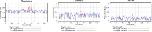
Under a volatile market environment, demand risk may be triggered by various external factors varying from new competitors, natural disasters or emerging disruptive technologies in the market (Shen and Li 2017; Ojha et al. 2018). For example, in 2019, warmer weather continuing into autumn adversely affected fashion retail demand in the UK, leading to an 80-million-pound loss every week (Met Office UK & British Retail Consortium 2019). In the context of COVID-19, Agricultural SCs faced a sudden fall in demand (post-panic-buying events) for their produce due to pandemic-related lockdowns (UK Parliament 2020). Based on Beccue et al.'s (2018) work, two states, one with a 25% reduction and a 50% reduction in market demand during weeks 72 and 110, were hypothesised for this disruption scenario. These states can best reflect real-world situations during lockdowns for a restricted period in a selected three-year (156 weeks) time horizon. Figure 3 shows the impact of 25 and 50% reduction in market demand on manufacturer, distributor and retailer nodes.

Figure 3. Supply chain disruption propagation due to demand risk.

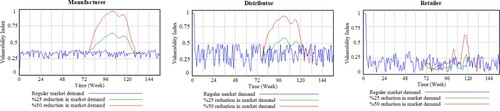
It is observed that a reduction in the market demand does not impact the retailer node in the immediate term. However, the severity of the variation in demand is felt later as the disruption propagates along the SC. As the closest entity to the market demand, the retailer node tends to be little impacted on its overall vulnerability index, with the setting time to form the expectation (three weeks in this model). However, it is observed that this cascades into increased inventory levels at the distributor as the average network demand decreases. Under this situation, the distributor has to deal with a higher vulnerability index in terms of obsolete or backlogged inventory.

Due to the ripple effect, disruption caused by demand risk further propagates upstream to the manufacturer and beyond in the SC. Interestingly, the impact of disruption is also delayed compared to the previous downstream node, owing to the delay in forming demand expectations between each node. According to Dolgui, Ivanov, and Sokolov (2018), a phenomenon called ‘distortion information of market demand variation’ exists. As the initial node of the SC system, the supplier tends to fail to respond to risk with timely remedies, increasing the inability to meet the manufacturer's demand. Reasons why this phenomenon occurs can be attributed to uncertain factors during disruption propagation, such as delay and distortion of information.

5.2. Disruption due to logistics risk

Sufficient transport capacity is vital at each SC entity, which ensures product movement and on-time delivery. In the wake of the COVID-19 pandemic, a critical shortage of containers drove up shipping costs (up to 300%) and delayed deliveries for goods purchased from China and other Asian regions (Tan 2021). This section simulates a situation associated with transportation capacity problems at the manufacturer node and its effects on various risk factors at different SC levels. Under these scenarios, the cause of disruption on transport capacity can be associated with driver strikes, vehicle damage or other contingencies (Qazi et al. 2018). An example of logistics disruption is the UK–EU border chaos during the spread of a new variant of COVID-19 combined with the confusion associated with ‘Brexit’ (The Economist 2020).

To provide a similar opportunity for comparing the previous scenario, we considered 25 and 50% decrease in the transport capacity between weeks 72 and 110. Figure 4 illustrates that the manufacturer shipping capacity decreases with increasing transport disruption with changes in different risk parameters. It is observed that the disruption tends to cause an impact on the entire SC, impacting the retailer to the highest extent (considering percentage change in vulnerability index), with delay or shortages in stock for meeting end customers’ demands. Figure 4 also illustrates the influence of the disruption impact on the distributor.

Figure 4. Supply chain disruption propagation due to logistics risk.

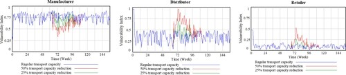
Transport capacity risk derived from the manufacturer propagates to the distributor by affecting its inventory level. Shipping capacity decrease leads to an increase in the inventory levels; however, this disruption is not felt immediately or in the short term by the manufacturer. It is rather observed to be affecting distributor and retailer significantly due to lack of inventory replenishments from the manufacturer. The results also show that the disruption impacts the retailer node slower than the distributor node, illustrating the cascading characteristic of the ripple effect.

5.3. Disruption due to supply risk

As the starting upstream node of the SC system, variations in supplier operations tend to influence the SC holistically by affecting various factors attached to the subsequent echelons of the network. The stability of the supplier’s supply level can directly or indirectly impact the key SC indicators such as inventory level, transport capacity, production and sales level. This section simulates a scenario with 25 and 50% reduction in supply quantity between weeks 72 and 110, typically caused by operational risks of labour, machines or damage to inventory from fires or natural disasters faced by the supplier. For example, during early COVID-19, multiple agri-food producers/suppliers could not harvest the food (e.g. fruits) primarily due to labour shortages in the UK, leading to huge food loss and waste (The Guardian 2020).

Predictably, the effect of disruption will first propagate to the manufacturer in the SC. For example, Figure 5 illustrates that the manufacturer (processor) faces inventory shortages and cannot achieve the planned production quantity due to disruption cascaded from the supplier. For distributor and retailer nodes, there is a marginal disruption impact caused due to 25 and 50% supply reduction.

Figure 5. Supply chain disruption propagation due to supply risk.

Simulation results demonstrate that the ripple effect propagates simultaneously further downstream nodes of the SC. Since both distributor and retailer tend to suffer inventory shortages almost concurrently, resulting in unanticipated and adverse impact in terms of lost sales and decreased customer satisfaction. Eventually, this can result in a loss of profit and even customer loyalty, negatively affecting the entire SC performance. It is anticipated that the risk exposure level at each node is likely to vary owing to the different degree of risk-resistant competencies owned by an individual node.

5.4. Disruption due to simultaneous risks

This scenario simulates the situation with three risks (supply quantity, transport capacity and market demand) occurring simultaneously. This risk scenario is particularly important, as it helps to understand and compare the ripple effect caused by individual and multiple disruption scenarios. For example, automotive and electronics industries have experienced an unprecedented shortage of semiconductors in the first quarter of 2021, leading to production halts and delivery delays through the ripple effect (Shead 2021). The reasons for these shortages were an unexpected increase in demand at automotive firms that recovered after the pandemic shock in 2020. However, the semiconductor suppliers have re-allocated their capacities to other SCs to benefit from their increasing demand for semiconductors and substitute the missing demand from the automotive industry. This example illustrates interconnections between different SC risks (e.g. natural resource shortage risks, demand risks, process risks and supply risks) along with the ripple effect (i.e. propagation of a local disruption through a global network), bullwhip effect (i.e. amplification of variations in production and order quantities across the SC induced by insufficient demand transparency) and intertwining of supply networks.

Through the variable-controlling approach (Wu, Blackhurst, and O’Grady 2007), the basic settings are the same as described in earlier sections. Three conditions, i.e. normal vulnerability, moderate vulnerability (Multiple scenario-1) and high vulnerability (Multiple scenario-2), were considered. By simulating this unique scenario, we can observe that multiple risk-driven disruptions cause a larger cascading impact on every SC node than a stand-alone disruption (Figure 6). For the manufacturers, as they receive less raw material from the suppliers, their production and inventory risk tend to increase, entailing some degree of transport risk and leading to further escalation of inventory/production risk. Similar observations are made at the retailer in terms of the vulnerability index. Inventory and sales risk increases at the retailer, as it receives insufficient quantities from the distributor, resulting from the supply shortages disruption and disruption in transport capacity and manufacturer production quantity at upstream SC nodes. Finally, this combined ripple effect of multiple disruptions on a multi-echelon SC propagates to the end customers in terms of unfulfilled demand and reduced service level.

Figure 6. Supply chain disruption propagation due to multiple, simultaneous risks.

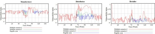
The results observed in Figure 6 also show that, compared with the distributor, the retailer and manufacturer tend to be more fragile in the SC because of multiple SC activities occurring at these two specific nodes, representing a higher vulnerability index. This observation provides strong evidence for inconsistent behaviour of disruption propagation within the SC network. However, it is difficult to generalise this insight as it may vary depending on SC nodes’ characteristics and the kind of disruption scenarios considered. Additionally, due to the cascading effect of multiple risks acting simultaneously, the standard deviation of the vulnerability index increases significantly in these scenarios, creating a highly vulnerable environment for the breakdown of the entire SC network.

6. Discussion

In this study, we examined the ripple effect in SCs under different scenarios of long-term, simultaneous disruptions induced by the COVID-19 pandemic. Our main aim was to uncover the value of the SD approach for the ripple effect recognition and visualisation, along with the analysis of dynamic production–supply behaviours at different SC echelons. We studied four disruptions scenarios induced by demand risk, logistics risk, supply risk and multiple simultaneous risks. To close the identified research gap, we analysed an understudied dynamic problem setting when disruptions occur in demand, supply and transport capacity individually and simultaneously over a longer time horizon. We developed an SD model and simulated the ripple effect in SCs, considering the multi-echelon system faced with varying disruptions felt across the SC. It has been observed that, without considering risk mitigation policies in the simulation model, the risk exposure level tends to accumulate over time as disruption propagates along the SC. The disruption scenario results with demand risk confirm that risk propagation starts downstream in the SC and propagates upstream.

Transport risk-driven disruption originating from the manufacturer tends to impact retailers to the greatest extent and is faced with the utmost inventory risk exposure level. The impact of this risk tends to accumulate across the SC, as it propagates further upstream. Comparing four risk scenarios, disruption propagation follows the bi-directional flow-upstream and downstream direction of the SC. The ripple effect of reduced inventory level leads to inventory risk at each node, as it cascades through the SC, finally resulting in decreased lost sales and poor customer satisfaction.

Simultaneous, multiple disruptions generate larger ripples across the SC compared to individual disruptions. Being exposed to more complex SC activities, the retailer and manufacturer tend to be more fragile under multiple disruptions in this simulation model. Furthermore, disruption propagation impact is significantly higher at each SC node for simultaneous risks over a longer time horizon. This is aligned with the general understanding that the ripple effect cascades with increasing effect across the SC network (Ojha et al. 2018).

Our SD simulation model enabled quantification and visualisation of the ripple effect in the SC. This dynamic modelling approach can help companies foresee risk exposure levels at the node and across the SC network. Our study results indicate that disruption propagation impact varies based on risk type, combination of risks and impacting node. It was also observed that longer duration disruptions typically suffer a larger overall impact on the wider SC. The ripple effect of any disruption is felt immediately but continues to impact over a longer duration unless the system attempts to recover from it. The impact of any disruption typically follows ‘disruption curve’ as described by Sheffi and Rice Jr (2005), where the extent of disruption impact and recovery is driven by several factors, such as time duration, type of risk, the inherent resilience of the node, mitigation actions, etc. Interestingly, in the case of pandemic risk (COVID-19), this disruption curve was observed to be following a ‘recurring wave’ pattern due to multiple lockdowns (i.e. opening and closure of SC nodes) impacting SC operations with a varying set of disruptions.

7. Conclusion and future research

7.1. Contribution to practice

Our study provides strong implications for practice. Following a structured research design, this study defined, applied and demonstrated the capability of SD modelling for visualising the behaviour of disruption propagation. Quantification of the ripple effect is crucial for understanding the complex behaviour of risks/disruptions in SCs (Dolgui, Ivanov, and Sokolov 2018; Zobel et al. 2021). However, the scenario-based simulation analysis conducted in this paper provides the opportunity to picture the SC disruption propagation phenomenon from macro-and micro-level perspectives. It is evident from the analysis that the ripple effect is influenced by several factors ranging from market–supply–demand–logistics characteristics, combination of disruptions and points of failure within the SC. Generated evidence-based information on influential variables and vulnerability index can better manage SC networks during future disruptions.

The developed simulation model for disruption propagation is robust and realistic to support the managers with the identification and recognition of weak nodes by identifying potential vulnerabilities across the network following a ‘system-wide view’. The visual representation of the ripple effect provided in this study is beneficial for building digital SC network models. Such simulation models can support in building a ‘digital twin’ of global SC networks for holistic assessment and mitigation (Ivanov and Dolgui 2020; Frazzon, Freitag, and Ivanov 2021). The analysis of possible risk-driven disruption scenarios is expected to help practitioners re-design risk-resistant SC structures and develop effective risk mitigation policies.

7.2. Contribution to theory

This study makes some useful contributions to the theory. This study contributes to the SCRM literature by examining the ripple effect in SCs under different scenarios of long-term, simultaneous disruptions induced by the COVID-19 pandemic. The ripple effect in the SC has attained well-established understanding; however, to the best of the author's knowledge, modelling this phenomenon following an SD approach and in the setting of long-term, simultaneous disruptions (e.g. like those induced by the COVID-10 pandemic) is the first of its kind. Although disruption scenarios have been considered in the literature using simulation modelling approach (e.g. Olivares-Aguila and ElMaraghy 2020), the SD simulation model developed to quantify and visualise the multi-layered effect due to disruption propagation on the SC network provides a unique methodological contribution, showcasing the potential of SD modelling for simulating a complex, dynamic phenomenon in an SC environment. Established bi-directional, increasing impact of disruption propagation across SC nodes is valuable insight and is expected to encourage SCRM researchers to explore further the behavioural dynamics of risks and associated cascading disruptions across SC networks.

7.3. Limitations and future research

Limitations exist, as with any other study. Secondary data were used to provide a general picture of the common risks occurring along an SC. The lack of primary data and subjectivity in some model parameters limit comprehensive quantification of the ripple effect. Another limitation resides in excluding cost factors and consideration of risk mitigation activities to recover from the disruption(s). Each scenario-based simulation was run only once with the limited number of iterations, thus it is difficult to generalise the findings. Growing globalisation, increasing collaboration and technology development (as part of Digitalisation and Industry 4.0) will lead to the emergence of new risks such as counterfeits, cybersecurity, systemic risk, etc. (Ghadge et al. 2020). Therefore, it is evident that the SC risk/disruption propagation research area will receive increased attention from both the academic community and the business environment post-COVID-19 pandemic.

Our study did not consider the conventional SC risk assessment (probability versus impact) approach. Instead, we used a vulnerability index to capture the disruption propagation phenomenon. This is believed to be an appropriate approach for ‘Black swam’ events (e.g. COVID-19 pandemic, Brexit and other natural and geo-political events), where conventional SCRM principles for risk assessment may not necessarily apply. Further study in this direction may provide additional clarity. Another research extension may consider information flow in the SC, exploring how the ripple effect influences the bullwhip effect (Dolgui, Ivanov, and Rozhkov 2020a). Ripple effect analysis in viable SC designs (Ivanov 2020) and reconfigurable SCs (Dolgui, Ivanov, and Sokolov 2020b) can shed light on some new and understudied mechanisms of the disruption propagation. It may also be interesting to investigate the propagation of risks in multi-channel SC networks and intertwined supply networks.

Disclosure statement

No potential conflict of interest was reported by the author(s).

Data availability statement

The data that support the findings of this study are available from the corresponding author [A. Ghadge] upon reasonable request.

Additional information

Notes on contributors

Abhijeet Ghadge

Abhijeet Ghadge is an Associate professor of Supply Chain Management at Cranfield School of Management, UK. He holds PhD in Operations and Supply Chain Management from Loughborough University, UK, and MTech in Industrial Engineering and Management from Indian Institute of Technology, India. He has over 14 years of industrial, academic and consulting experience working with a wide range of UK, European and Asian organisations. Dr Ghadge has published over 70 research papers, including 40 journal articles in leading operations, logistics and supply chain management journals. He follows practice-driven approach to problems across the broad domains of supply chain risk, sustainability and Industry 4.0.

Merve Er

Merve Er is an Assistant Professor in the department of Industrial Engineering at Marmara University, Turkey. She holds BS, MS and PhD degrees in Industrial Engineering. She was a Postdoc at Heriot-Watt University in UK between April 2018–March 2019 and supported by international post-doctoral research scholarship program of the Scientific and Technological Research Council of Turkey (TUBITAK). Her main research interests include Supply Chain Risk Management, Performance Management, Simulation and Modelling, and Ant Colony Optimisation. She has published widely and participated in several industry and government projects.

Dmitry Ivanov

Dmitry Ivanov is a full professor of supply chain and operations management at Berlin School of Economics and Law (HWR Berlin). His achievements have been recognised by numerous research and teaching awards. His publication record counts around 360 publications, including 111 papers in international academic journals (e.g. ANOR, EJOR, IEEE-TEM, IISE Transactions, IJPE, IJPR, Omega and TRE: Part E) and leading textbooks Global Supply Chain and Operations Management and Introduction to Supply Chain Resilience. His main research interests and results span the resilience and ripple effect in supply chains, risk analytics and digital supply chain twins. His projects have been supported by funding from European Commission (H2020), DFG (German Research Foundation), DAAD, IFAF Berlin, Norwegian Research Council, Alexander von Humboldt-Foundation as well industrial companies. He delivered invited plenary, keynote and panel talks at conferences of INFORMS, IFPR, DSI, POM, IFAC and IFIP. He co-edits International Journal of Integrated Supply Management (IJISM) and is an associate editor of the International Journal of Production Research (IJPR). He is the Chairman of IFAC TC 5.2 ‘Manufacturing Modelling for Management and Control’

Atanu Chaudhuri

Atanu Chaudhuri is an Associate Professor of Operations and Technology Management at Durham University Business School, UK, and an Adjunct Associate Professor of Operations and Supply Chain Management at Aalborg University, Denmark. Dr Atanu obtained his PhD in Operations Management from Indian Institute of Management, Lucknow. Dr Atanu has more than 8 years of industrial experience having worked in automotive industry, consulting and research – all in India and more than 10 years of academic experience in India (Indian Institute of Management, Lucknow), Denmark (Aalborg University) and UK (Durham University). He has more than 40 journal articles to his credit and has published in leading journals. His research focuses on supply chain implications of additive manufacturing, supply chain risk management and resilience. He is the Senior Associate Editor of International Journal of Logistics Management. His research has been funded by UKIERI, Innovation Fund-Denmark, Danish Agency for Science and Higher Education and TUBITAK.

Appendices

Appendix 1

Numerical settings for simulation

Start week=0, final week=156, time interval=1 week (Units: week).

Average market demand=50 thousand units/week, changing with 70–130% variation, which starts from week 4.

Time to form demand expectations at each SC entity = 3 weeks.

The weight of supplier risk: inventory risk=0.6, transport risk=0.4.

The weight of manufacturer risk: production risk=0.5, inventory risk=0.3, transport risk=0.2.

The weight of distributor risk: inventory risk=0.6, transport risk=0.4.

The weight of retailer risk: sales risk=0.5, inventory risk=0.3, transport risk=0.2.

Initial inventory level for each SC entity=20 thousand units.

Expected inventory level at each SC entity=55 thousand units.

The supply/production/distribute/sales capacity at each specific SC entity: Range [30, 60 (upper limit)] (unit: thousand units).

Vehicle capacity (same for all SC entities) = 2.5 thousand units/car (To distinguish, vehicle capacity constant variables at each node are named with 1,2,3,4 in the stock and flow diagram).

Vehicle volume at each SC entity: Range [15,25] (unit: car).

Inventory adjustment

=Time ([(0,0) −(156,10)], (0,0), (20,0), (30,0), (40,0), (50,0.35), (60,0), (100,0), (156,0))

0.35 represents the inventory adjustment will take effect on week 50 with 35% inventory volume decreased.

Vehicle volume adjustment

=Time ([(0,0) -(156,10)], (0,0), (20,0), (30,0), (40,0), (50,0.35), (60,0), (100,0), (156,0))

0.35 represents the vehicle volume adjustment will take effect on week 50 with 35% vehicle volume decreased.

Equations used in SD model

Supplier actual inventory = Supplier supply quantity − Supplier capacity

Manufacturer actual inventory = Manufacturer supply quantity − production quantity

Distributor actual inventory = Distributor distribute quantity − Distributor capacity

Retailer actual inventory = Retailer sales quantity − Retailer sales capacity

Shipping capacity = Vehicle capacity × Vehicle volume (Same for all nodes)

If actual inventory = expected inventory, then inventory risk=0; Else, inventory risk = Absolute value of (actual inventory − expected inventory) / expected inventory (Same for all nodes)

If actual output quantity<=shipping capacity, transport risk=0; Else, transport risk= (Actual output quantity-shipping capacity) / Output quantity (Same for all nodes)

If production quantity>=planned production quantity, production risk=0; Else, production risk= (Planned production quantity – production quantity) / Planned production quantity

If sales quantity>=Planned sales quantity, sales risk=0; Else, sales risk= (Planned sales quantity – sales quantity) / Planned sales quantity

Vulnerability index = 0.6 × Inventory risk + 0.4 × Transport risk (Applicable for supplier and distributor node in SC)

Vulnerability index = 0.5 × Production (or) Sales risk + 0.3 × Inventory + 0.2 × Transport risk (Applicable for manufacturer and retailer node in SC)

Appendix 2

Validation tests for SD models

• Relevance test: This is a simple test to check the influencing variables are correctly linked to capture potential impact in the SD model. This was manually checked.

• Consistency test: This test is important as it checks that the computer model correctly replicates the behaviour of a real SC system. Although no benchmarking system was used to validate the SD model, we used authors knowledge in SC to confirm this.

• Sensitivity test: Parameter and structural consistency tests were conducted to test the behaviour of the SD model to reasonable variations in parameter values (by changing individual factor) and minor structural changes. This is extensively conducted in the study.

• Extreme condition test: This test is different from the sensitivity test, and checks if equations developed for the SD model (presented in Appendix 1) make sense and are logical. It also checks whether the model performs well to the extreme, but possible parametric values. This was done with the help of SD modelling expert.

References

- Basole, R. C., and M. A. Bellamy. 2014. “Supply Network Structure, Visibility, & Risk Diffusion: A Computational Approach.” Decision Sciences 45 (4): 753–789.
- Beccue, P. C., H. G. Huntington, P. N. Leiby, and K. R. Vincent. 2018. “An Updated Assessment of oil Market Disruption Risks.” Energy Policy 115: 456–469.
- Bueno-Solano, A., and M. G. Cedillo-Campos. 2014. “Dynamic Impact on Global Supply Chains Performance of Disruptions Propagation Produced by Terrorist Acts.” Transportation Research Part E 61: 1–12.
- Chauhan, V. K., S. Perera, and A. Brintrup. 2021. “The Relationship Between Nested Patterns and the Ripple Effect in Complex Supply Networks.” International Journal of Production Research 59 (1): 325–341.
- Choi, T., D. Rogers, and B. Vakil. 2020. “Coronavirus Is a Wake-Up Call for Supply Chain Management.” Harvard Business Review. March 27, 2020.
- Currie, C. S. M., J. W. Fowler, K. Kotiadis, T. Monks, B. S. Onggo, D. A. Robertson, and A. A. Tako. 2020. “How Simulation Modelling Can Help Reduce the Impact of COVID-19.” Journal of Simulation 14 (2): 1–15. 83–97.
- Deng, X., X. Yang, Y. Zhang, Y. Li, and Z. Lu. 2019. “Risk Propagation Mechanisms and Risk Management Strategies for a Sustainable Perishable Products Supply Chain.” Computers and Industrial Engineering 135: 1175–1187.
- Ding, Z., W. Gong, S. Li, and Z. Wu. 2018. “System Dynamics Versus Agent-Based Modeling: A Review of Complexity Simulation in Construction Waste Management.” Sustainability 10 (7): 2484.
- Dolgui, A., and D. Ivanov. 2021. “Ripple Effect and Supply Chain Disruption Management: New Trends and Research Directions.” International Journal of Production Research 59 (1): 102–109.
- Dolgui, A., D. Ivanov, and M. Rozhkov. 2020a. “Does the Ripple Effect Influence the Bullwhip Effect? An Integrated Analysis of Structural and Operational Dynamics in the Supply Chain.” International Journal of Production Research 58 (5): 1285–1301.
- Dolgui, A., D. Ivanov, and B. Sokolov. 2018. “Ripple Effect in the Supply Chain: An Analysis and Recent Literature.” International Journal of Production Research 56 (1–2): 414–430.
- Dolgui, A., D. Ivanov, and B. Sokolov. 2020b. “Reconfigurable Supply Chain: The X-Network.” International Journal of Production Research 58 (13): 4138–4163.
- The Economist. 2020. Christmas Chaos – How Covid-19 and Brexit Combined to Isolate Britain. https://www.economist.com/britain/2020/12/21/how-covid-19-and-brexit-combined-to-isolate-britain (accessed on 2 August 2021).
- El Baz, J., and S. Ruel. 2021. “Can Supply Chain Risk Management Practices Mitigate the Disruption Impacts on Supply Chains’ Resilience and Robustness? Evidence from an Empirical Survey in a COVID-19 Outbreak Era.” International Journal of Production Economics 233: 107972.
- Er Kara, M., A. Ghadge, and U. S. Bititci. 2020. “Modelling the Impact of Climate Change Risk on Supply Chain Performance.” International Journal of Production Research, 1–19, Online.
- Foerster, J. 1968. Principles of Systems. Cambridge: MIT Press.
- Frazzon, E. M., M. Freitag, and D. Ivanov. 2021. “Intelligent Methods and Systems for Decision-Making Support: Toward Digital Supply Chain Twins.” International Journal of Information Management 57: 102281.
- Ghadge, A., S. Dani, M. Chester, and R. Kalawsky. 2013. “A Systems Thinking Approach for Modelling Supply Chain Risk Propagation.” Supply Chain Management: An International Journal 18 (5): 523–538.
- Ghadge, A., S. Dani, and R. Kalawsky. 2012. “Supply Chain Risk Management: Present and Future Scope.” The International Journal of Logistics Management 23 (3): 313–339.
- Ghadge, A., S. K. Jena, S. Kamble, D. Misra, and M. K. Tiwari. 2020. “Impact of Financial Risk on Supply Chains: a Manufacturer-Supplier Relational Perspective.” International Journal of Production Research, 1–16, Online.
- Gholami-Zanjani, S. M., M. S. Jabalameli, W. Klibi, and M. S. Pishvaee. 2021. “A Robust Location-Inventory Model for Food Supply Chains Operating Under Disruptions with Ripple Effects.” International Journal of Production Research 59 (1): 301–324.
- Goldbeck, N., P. Angeloudis, and W. Ochieng. 2020. “Optimal Supply Chain Resilience with Consideration of Failure Propagation and Repair Logistics.” Transportation Research Part E: Logistics and Transportation Review 133: 101830.
- The Guardian. 2020. “A Disastrous Situation': Mountains of Food Wasted as Coronavirus Scrambles Supply Chain.” See https://www.theguardian.com/world/2020/apr/09/us-coronavirus-outbreak-agriculture-food-supply-waste (accessed on 2 August 2021).
- Haren, P., and D. Simch-Levi. 2020. “How Coronavirus Could Impact the Global Supply Chain by Mid-March.” Harvard Business Review 28.
- Heckmann, I., T. Comes, and S. Nickel. 2015. “A Critical Review on Supply Chain Risk – Definition, Measure and Modelling.” Omega 52: 119–132.
- Ho, W., T. Zheng, H. Yildiz, and S. Talluri. 2015. “Supply Chain Risk Management: A Literature Review.” International Journal of Production Research 53 (16): 5031–5069.
- Hosseini, S., and D. Ivanov. 2020. “Bayesian Networks for Supply Chain Risk, Resilience and Ripple Effect Analysis: A Literature Review.” Expert Systems with Applications 161: 113649.
- Ivanov, D. 2017. “Simulation-based Ripple Effect Modelling in the Supply Chain.” International Journal of Production Research 55 (7): 2083–2101.
- Ivanov, D. 2020. “Viable Supply Chain Model: Integrating Agility, Resilience and Sustainability Perspectives – Lessons from and Thinking Beyond the COVID-19 Pandemic.” Annals of Operations Research, doi:10.1007/s10479-020-03640-6.
- Ivanov, D., and A. Dolgui. 2020. “A Digital Supply Chain Twin for Managing the Disruption Risks and Resilience in the Era of Industry 4.0.” Production Planning & Control 32 (9): 775–788.
- Ivanov, D., B. Sokolov, and A. Dolgui. 2014. “The Ripple Effect in Supply Chains: Trade-off ‘Efficiency-Flexibility-Resilience’ in Disruption Management.” International Journal of Production Research 52 (7): 2154–2172.
- Janssen, S., A. Sharpanskykh, and R. Curran. 2019. “AbSRiM: An Agent-Based Security Risk Management Approach for Airport Operations.” Risk Analysis 39 (7): 1582–1596.
- Kamath, N. B., and R. Roy. 2007. “Capacity Augmentation of a Supply Chain for a Short Lifecycle Product: A System Dynamics Framework.” European Journal of Operational Research 179 (2): 334–351.
- Kinra, A., D. Ivanov, A. Das, and A. Dolgui. 2020. “Ripple Effect Quantification by Supplier Risk Exposure Assessment.” International Journal of Production Research 58 (19): 5559–5578.
- Li, Y., C. W. Zobel, O. Seref, and D. Chatfield. 2020. “Network Characteristics and Supply Chain Resilience Under Conditions of Risk Propagation.” International Journal of Production Economics 223: 107529.
- Llaguno, A., J. Mula, and F. Campuzano-Bolarin. 2021. “State of the art, Conceptual Framework and Simulation Analysis of the Ripple Effect on Supply Chains.” International Journal of Production Research, 1–23. doi:10.1080/00207543.2021.1877842.
- Lücker, F., S. Chopra, and R. W. Seifert. 2020. “Mitigating Product Shortages due to Disruptions in Multi-Stage Supply Chains.” Production and Operations Management, doi:10.1111/poms.13286.
- Macdonald, J. R., C. W. Zobel, S. A. Melnyk, and S. E. Griffis. 2018. “Supply Chain Risk and Resilience: Theory Building Through Structured Experiments and Simulation.” International Journal of Production Research 56 (12): 4337–4355.
- Martis, M. S. 2006. “Validation of Simulation-based Models: a Theoretical Outlook.” The Electronic Journal of Business Research Methods 4 (1): 39–46.
- Met Office and British Retail Consortium. 2019. https://brc.org.uk/news/2018/weather-to-shop (accessed on 2 August 2021).
- Mingers, J., and L. White. 2010. “A Review of the Recent Contribution of Systems Thinking to Operational Research and Management Science.” European Journal of Operational Research 207 (3): 1147–1161.
- Mula, J., F. Campuzano-Bolarin, M. Díaz-Madroñero, and K. M. Carpio. 2013. “A System Dynamics Model for the Supply Chain Procurement Transport Problem: Comparing Spreadsheets, Fuzzy Programming and Simulation Approaches.” International Journal of Production Research 51 (13): 4087–4104.
- Nagurney, A. 2021. “Supply Chain Game Theory Network Modeling Under Labor Constraints: Applications to the Covid-19 Pandemic.” European Journal of Operational Research, doi:10.1016/j.ejor.2020.12.054.
- Nilsson, F., and V. Darley. 2006. “On Complex Adaptive Systems and Agent-Based Modelling for Improving Decision-Making in Manufacturing and Logistics Settings: Experiences from a Packaging Company.” International Journal of Operations & Production Management 26 (12): 1351–1373.
- Ojha, R., A. Ghadge, M. Tiwari, and U. Bititci. 2018. “Bayesian Network Modelling for Supply Chain Risk Propagation.” International Journal of Production Research 56 (17): 5795–5819.
- Olivares-Aguila, J., and W. ElMaraghy. 2020. “System Dynamics Modelling for Supply Chain Disruptions.” International Journal of Production Research, 1–19. doi:10.1080/00207543.2020.1725171.
- Paul, S. K., and P. Chowdhury. 2020. “A Production Recovery Plan in Manufacturing Supply Chains for a High-demand Item During COVID-19.” International Journal of Physical Distribution & Logistics Management, doi:10.1108/IJPDLM-04-2020-0127.
- Pavlov, A., D. Ivanov, F. Werner, A. Dolgui, and B. Sokolov. 2019. “Integrated Detection of Disruption Scenarios, the Ripple Effect Dispersal and Recovery Paths in Supply Chains.” Annals of Operations Research, 1–23.
- Qazi, A., A. Dickson, J. Quigley, and B. Gaudenzi. 2018. “Supply Chain Risk Network Management: A Bayesian Belief Network and Expected Utility Based Approach for Managing Supply Chain Risks.” International Journal of Production Economics 196: 24–42.
- Rao, S., and T. J. Goldsby. 2009. “Supply Chain Risks: A Review and Typology.” The International Journal of Logistics Management 20 (1): 97–123.
- Rathore, R., J. J. Thakkar, and J. K. Jha. 2020. “Impact of Risks in Food Grains Transportation System: A System Dynamics Approach.” International Journal of Production Research, 1–20.
- Ruel, S., J. El Baz, D. Ivanov, and A. Das. 2021. “Supply Chain Viability: Conceptualization, Measurement, and Nomological Validation.” Annals of Operations Research, doi:10.1007/s10479-021-03974-9.
- Scheibe, K. P., and J. Blackhurst. 2018. “Supply Chain Disruption Propagation: a Systemic Risk and Normal Accident Theory Perspective.” International Journal of Production Research 56 (1–2): 43–59.
- Shead, S. 2021. “Carmakers Have Been Hit Hard by a Global Chip Shortage—here’s Why.” https://www.cnbc.com/2021/02/08/carmakers-have-been-hit-hard-by-a-global-chip-shortage-heres-why-.html (accessed on 5 March 2021).
- Sheffi, Y., and J. B. Rice Jr. 2005. “A Supply Chain View of the Resilient Enterprise.” MIT Sloan Management Review 47 (1): 41–48.
- Shen, B., and Q. Li. 2017. “Market Disruptions in Supply Chains: A Review of Operational Models.” International Transactions in Operational Research 24: 697–711.
- Singh, S., R. Kumar, R. Panchal, and M. K. Tiwari. 2020. “Impact of COVID-19 on Logistics Systems and Disruptions in Food Supply Chain.” International Journal of Production Research, doi:10.1080/00207543.2020.1792000.
- Sodhi, M., C. Tang, and E. Willenson. 2021. “Research Opportunities in Preparing Supply Chains of Essential Goods for Future Pandemics.” International Journal of Production Research, doi:10.1080/00207543.2021.1884310.
- Sokolov, B., D. Ivanov, A. Dolgui, and A. Pavlov. 2016. “Structural Quantification of the Ripple Effect in the Supply Chain.” International Journal of Production Research 54 (1): 152–169.
- Sterman, J. 2010. Business Dynamics: Systems Thinking and Modelling for Complex World. New York, USA: Irwin/McGraw-Hill Publishing.
- Svensson, G. 2002a. “A Typology of Vulnerability Scenarios Towards Suppliers and Customers in Supply Chains Based Upon Perceived Time and Relationship Dependencies.” International Journal of Physical Distribution and Logistics Management.
- Svensson, G. 2002b. “Dyadic Vulnerability in Companies' Inbound and Outbound Logistics Flows.” International Journal of Logistics 5 (1): 13–43.
- Swierczek, A. 2016. “The ‘Snowball Effect’ in the Transmission of Disruptions in Supply Chains the Role of Intensity and Span of Integration.” The International Journal of Logistics Management 27 (3): 1002–1038.
- Tako, A. A., and S. Robinson. 2009. “Comparing Discrete-Event Simulation and System Dynamics: Users’ Perceptions.” Journal of the Operational Research Society, Palgrave Macmillan; The OR Society 60 (3): 296–312.
- Tan. 2021. “An ‘aggressive’ Fight over Containers Is Causing Shipping Costs to Rocket by 300%.” https://www.cnbc.com/2021/01/22/shipping-container-shortage-is-causing-shipping-costs-to-rise.html (accessed on 2 August 2021).
- UK Parliament. 2020. Effects of COVID-19 on the food supply system. https://post.parliament.uk/effects-of-covid-19-on-the-food-supply-system/ (accessed on 5 March 2021).
- Wagner, S. M., and N. Neshat. 2010. “Assessing the Vulnerability of Supply Chains Using Graph Theory.” International Journal of Production Economics 126 (1): 121–129.
- Wilson, M. C. 2007. “The Impact of Transportation Disruptions on Supply Chain Performance.” Transportation Research Part E: Logistics and Transportation Review 43 (4): 295–320.
- Wu, T., J. Blackhurst, and P. O’Grady. 2007. “Methodology for Supply Chain Disruption Analysis.” International Journal of Production Research 45 (7): 1665–1682.
- Zobel, C. W., C. A. MacKenzie, M. Baghersad, and Y. Li. 2021. “Establishing a Frame of Reference for Measuring Disaster Resilience.” Decision Support Systems 140: 113406.