Single-machine scheduling with energy generation and storage systems

ABSTRACT

This paper considers a single-machine scheduling problem with sequence-dependent setup times and energy-generation and storage systems. Each job requires a sequence-dependent setup to be processed on the machine, and both setup and processing of the job require job-dependent amounts of energy. The energy consumed by the machine can be bought from an Electric Power Company (EPC) or generated by own Distributed Energy Resource (DER), such as solar photovoltaic or wind, and the energy can be stored in an Energy Storage System (ESS). The objective is to minimise the total cost, the sum of production cost depending on makespan and energy cost by considering energy usage from the EPC, DER and ESS. For the problem, a mathematical programming model is first derived by using period-based indexes. Then, a hybrid genetic algorithm, which adds appropriate idle times between jobs and determines an efficient energy schedule by storing some energy during less expensive periods into the ESS for later use in high-price periods, is developed. Finally, computational experiments show that the proposed algorithm provides effective solutions, and which component of the total cost affects the performance the most, how effective adding idle times between jobs is, and how much cost can be saved by having a DER and ESS.

KEYWORDS:

• Scheduling
• distributed energy resource
• energy storage system
• genetic algorithm
• sequence-dependent setup time

1. Introduction

A significant proportion of energy used in manufacturing is currently generated through fossil fuels (Rahimifard, Seow, and Childs 2010). Although the current oil prices suggest an abundance of resources, increasing population and energy wastage put the world at risk of an energy crisis in the near future. Indeed, the European Union has started developing contingency plans to deal with foreseen disruptions to the energy supply, and the UN considers sustainable energy to be a crucial element of global development (UN Sustainable Development 2020). The manufacturing sector uses tremendous amounts of energy and produces a half of the world's CO${}_2$ emissions (OECD-IEA 2019); because of resource scarcity and increasing greenhouse gases from production processes, energy efficiency will become a major consideration for manufacturing in the foreseeable future.

To respond to this, there have been enormous efforts by energy suppliers as well as manufacturing companies in energy-intensive industry, such as steel, chemicals, and aluminium (Araceli, Peter, and Tiffany 2019). On the energy suppliers' side, Time-of-Use (ToU) tariffs on retail electricity prices are widely used to manage the balance between supply and demand and to improve the reliability and efficiency of electrical power grids. For example, as one of the largest electric energy companies in South Korea, Korea Electric Power Corporation (KEPCO), offers ToU plans that charge higher prices for peak hours and considerably lower prices otherwise. Table 1 shows ToU tariffs applied to a customer with the contract demand of 300 kW or more, high-voltage, and less than 500 hours of use, depending on the season and time. On the manufacturers' side, efforts include the growing use of renewable energy from Distributed Energy Resources (DERs) – such as solar photovoltaics (PV) or wind turbines – and the installation of an Energy Storage System (ESS). Recently, many manufacturing companies have started operating their own DERs and ESSs according to their production schedule in order to reduce energy costs and greenhouse gas emissions.

Table 1. An example of ToU tariff.

Classification		Spring & Fall (3-5, 9-10)	Summer (6-9)	Winter (11-2)
Off-peak	Time	23:00-09:00		23:00-09:00
	Cost (KRW/kW)	56.1	56.1	63.1
Mid-peak	Time	09:00-10:00, 12:00-13:00, 17:00–23:00		09:00–10:00, 12:00–17:00, 20:00–22:00
	Cost (KRW/kW)	78.6	109	109.2
On-peak	Time	10:00–12:00, 13:00–17:00		10:00–12:00, 17:00–20:00, 22:00–23:00
	Cost (KRW/kW)	109.3	191.1	166.7

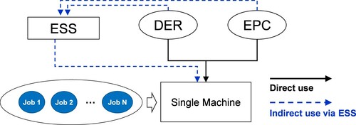
This paper considers a single-machine scheduling problem with sequence-dependent setup times together with energy-generation and storage systems. When switching from one job to another on a machine, a setup is required, and the setup time is sequence-dependent. Job processing and setup operations require a certain amount of (usually electrical) energy; a different amount of energy is required by each job, and a setup generally consumes less energy than job processes. The energy consumed by the machine can be bought from an Electric Power Company (EPC) or generated by the manufacturer's own DER. In addition, the energy from the EPC or DER can be stored in an ESS and used later when the electricity price is high (as in Figure 1). The objective is to minimise the total cost, the sum of the production and energy costs. The production cost is computed with makespan multiplied by a unit production cost; the energy cost is the sum of the energy price from the EPC, a generation cost from the DER, and the charging and discharging costs of the ESS.

Figure 1. An illustration of the energy flow. An image that shows the energy flow in a production system with ESS, DER, and EPC.

This work originated with research in a South Korean company that casts various automotive pistons. Molten aluminium alloy is poured into a mould with a hollow cavity of the desired shape for each piston before being solidified in a casting machine. Switching piston types requires a setup operation of several hours; the setup time depends on the piston type to be processed and the piston type previously processed on the same machine. A casting machine consumes a large amount of energy, and the energy consumption rate is different for each piston type (Salonitis et al. 2016). In the factory, there are several casting machines with different capacities, configurations, and functions, and almost all machines are already dedicated to specific product types according to special customer requirements, quality standards, and material types. Hence, a certain piston type can only be processed on a very limited number of certain machines – often only one or two. For example, most types of piston for BMW are only processed on a single machine in the company.

Another application can be found in a South Korean company that produces fan filter units (FFUs) used for purifying and supplying clean air in semiconductor and LCD manufacturing. Different aluminium alloy sheets go through clinching and riveting processes on a machine before being assembled with fans (by workers and robots) and packaged. The clinching and riveting machine requires a setup operation when changing products; the setup time depends on the tools used and the sizes of the previous and subsequent products. The machine's energy consumption for setups and processes also depends on products. The company consumes as much as 6000–8000 kW per day and has a solar PV power generation system with a capacity of 300 kWh. About 5–20% of the total energy used is provided by the DER, depending on the season. It also has an ESS to store the energy generated by the DER, or bought from the EPC when the electricity price is low, to be used during the peak-load price time. A simple example of a single machine with two jobs, denoted as Example 1, is provided in the supplementary material.

Literature review is presented in Section 2, and notations and a mathematical programming model are introduced in Section 3. Then a hybrid genetic algorithm (GA) is developed in Section 4, and computational experiments to evaluate the performance of the proposed heuristic is conducted in Section 5. Some concluding remarks and directions for future research are given in Section 6.

2. Literature review

There have been numerous papers on single-machine scheduling with sequence-dependent setup times (Ovacikt and Uzsoy 1994; Lee, Bhaskaran, and Pinedo 1997; Liao and Juan 2007). Recently, Vélez-Gallego, Maya, and Montoya-Torres (2016) proposed a mixed integer programming (MIP) model and a beam search heuristic with release dates, and Mustu and Tamer (2018) considered learning effects and sequence-dependent setup times simultaneously. A review on scheduling with sequence-dependent setup times can be found in Zhu and Wilhelm (2006).

The previous papers on scheduling production systems mostly focus on increasing throughput, reducing lead times, or satisfying due dates. There have recently been a few papers that consider energy usage in scheduling problems. Yildirim and Mouzon (2012) handled single-machine scheduling to minimise energy consumption and total completion time and proposed a multi-objective GA for deriving a set of non-dominated solutions. Shrouf et al. (2014) proposed a mathematical model and a GA to minimise energy consumption costs for single-machine production scheduling. Gong et al. (2015) examined a single-machine scheduling problem for minimising the energy cost without exceeding the due date and proposed a MIP model. Che, Zeng, and Lyu (2016) addressed an energy-aware single-machine scheduling problem under the ToU electricity tariffs to minimise the total electricity cost with a given deadline. They proposed a MIP model and an efficient greedy insertion heuristic where jobs are inserted into the time periods with the minimum electricity cost. Che, Zhang, and Wu (2017) considered a power-down mechanism in a single-machine scheduling problem where the machine can execute a power-down operation between two consecutive jobs. The objective is to minimise both total energy consumption and maximum tardiness. Wang et al. (2016) examined energy-efficient single-machine scheduling for batch production in order to minimise makespan and total energy cost and proposed an exact ϵ-constraint method and two heuristic methods to obtain Pareto fronts. Aghelinejad, Ouazene, and Yalaoui (2018) considered a single-machine scheduling problem to minimise the total energy cost. In the problem, three operating states, processing, shutdown, and idle, and two transitions for turning the machine on and off were assumed. Rubaiee and Yildirim (2019) used an ant colony optimisation (ACO) algorithm for single-machine preemptive scheduling to minimise the total completion time and energy cost. Most papers on single-machine scheduling with energy have not considered sequence-dependent setup times or energy usage during setup operations. In addition, the DER or ESS has not been handled together with production scheduling.

There have also been some studies on energy-conscious scheduling for other machine configurations, such as parallel machines, flow shops, and job shops. Moon, Shin, and Park (2013) considered unrelated parallel machine scheduling with time-dependent and machine-dependent electricity costs and proposed a hybrid GA combined with a blank job insertion algorithm. Moon and Park (2014) addressed flexible job shop scheduling without setups in order to minimise the total production cost and electricity cost. Liu et al. (2016) dealt with a multi-objective job shop scheduling problem to optimise energy consumption and production performance using a GA. Ding et al. (2016) examined unrelated parallel machine scheduling under ToU electricity prices with an objective of minimising the total electricity cost with a given production deadline. Tang et al. (2016) used the particle swarm optimisation (PSO) for energy-efficient dynamic scheduling of flexible flow shops to reduce energy consumption and makespan. Luo, Zhang, and Yushun (2019) considered flexible job shops with variable processing speeds with grey wolf optimisation (GWO). Che, Zhang, and Wu (2017) addressed the same problem in Ding et al. (2016), updated the MIP model, and proposed a two-stage heuristic algorithm. Cheng, Chu, and Zhou (2018) also improved the MIP formulation in Ding et al. (2016) and compared the two models with CPLEX. Merkerts et al. (2015) presented major challenges of combining scheduling and energy management, and Gahm et al. (2016) and Gao et al. (2020) reviewed papers on energy-efficient scheduling in manufacturing systems.

Most studies on machine scheduling with energy have tried to minimise energy consumption without considering changing electricity prices or to minimise the total energy cost under ToU tariffs. Many of them have used two objectives, production performance, such as makespan or tardiness, and energy efficiency, such as total energy consumption or energy cost, and developed heuristic algorithms. However, they have not considered setup operations or setup energy consumption as well as the DER or ESS. To the best of our knowledge, there was only one paper that assumed the DER and ESS in production scheduling, but it did not consider setups, and the energy from the DER is not stored in the ESS (Moon and Park 2014). They used constraint programming (CP) and MIP approaches to solve the problem.

Note that many studies have used a GA for scheduling problems because the GA is easy to understand and implement and shows acceptable performance in general. However, many previous studies only determine the job sequence with the various objectives, such as makespan, total completion time, and maximum lateness. Moreover, most works on energy-efficient scheduling problems assign jobs to certain periods and determine their sequence without considering the ESS or DER. Therefore, it is challenging to consider the ESS charging/discharging schedules and DER generation schedule in the GA. We hence propose a hybrid GA that can determine not only the assignment and sequence of jobs but also the ESS and DER schedules. The GA is suitable for representing a sequence of jobs on the single machine as a solution and for obtaining a good schedule by extracting important features of solutions and passing them down to the next generation while carrying a set of multiple solutions (Vallada and Ruiz 2011; May et al. 2015; Zhang and Chiong 2016). Other meta-heuristic algorithms, such as the PSO, artificial bee colony (ABC), gravitational search algorithm (GSA), and GWO, can also be used for the problem. However, sophisticated algorithm designs are required for obtaining ESS and DER schedules.

Three main contributions of this study are as follows. First, single machine scheduling, which considers setup energy consumptions, ESS, and DER simultaneously, is considered for the first time, and the corresponding mathematical programming model is presented. Second, a hybrid GA composed of an idle time generation algorithm, which appropriately inserts a certain amount of idle times before each job if it decreases the total cost, and an energy scheduling algorithm, which determines energy usage from the EPC, DER, and ESS is proposed. Third, various experiments are performed to show the effectiveness of the proposed algorithm, performance of the idle time generation algorithm, and efficiency of having the DER and ESS.

3. Problem description

There is a set of jobs $J=\{1,\dots ,N\}$ to be processed in a single machine, which is available at time 0. Job $j\in J$ requires processing on the single machine for uninterrupted $p_j$ time units, and a setup is conducted for $s_{ij}$ time units when it is processed after job $i\in J$. Let $a_j$ and $b_j$ denote the amount of energy required for processing and setup of job j, respectively. The total amount of energy spent by job j is equal to $a_j{p}_j+b_j{s}_{ij}$. There is no energy consumption when the machine is idle. The time horizon is partitioned into $T\ge 2$ periods $\mathcal{T}=\{1=[{\tau }_0,{\tau }_1],\dots ,T=[{\tau }_{T-1},{\tau }_T\left]\right\}$ where ${\tau }_0=0$, and ${\mathrm{\Delta }}_t={\tau }_t-{\tau }_{t-1}>0$ is the duration of period t for $t=1,\dots ,T$. Note that the processing (or setup) of a job can be incurred across two or more adjacent periods. The actual processing (or setup) time of a job in period t denotes the amount of time in period t used for processing (or setup) of the job. Note that ${\mathrm{\Delta }}_t$, $\mathrm{\forall }t$, is usually 60 (minutes) in practice because the weather forecast or electricity price is provided in an hour unit.

A DER generation cost per kW in period t is denoted as $g_t$, and the maximum amount of energy that can be generated from the DER in period t is represented with ${\overline{DER}}_t$. Note that $g_t$ is mostly the same regardless of period t, and ${\overline{DER}}_t$ is predicted based on weather forecast. An ESS has the storage capacity of $\overline{ESS}$, and an amount of energy stored in the ESS for all periods should be within the range of [$\alpha \overline{ESS},\text{β}\overline{ESS}$] due to an ESS operational efficiency issue where $\alpha ,\text{β}\in [0,1],\alpha <\text{β}$. The maximum amount of energy that can be charged into or discharged from an ESS in a period is denoted as $\overline{EC}$ or $\overline{ED}$, respectively. Charging and discharging costs per kW are represented with c and d, respectively. It is assumed that charging and discharging in the ESS cannot occur at the same time (Moon and Park 2014). The parameters and decision variables in the problem are:

Parameters

$p_j$	=	processing time of job j.
$s_{ij}$	=	setup time of job j after job i.
f	=	production cost per unit time.
${\overline{s}}_j$	=	$\underset{0\le i\le n}{max}$ $s_{ij}$.
${\overline{SE}}_j$	=	the maximum number of periods that a setup operation for job j can span.
${\overline{PR}}_j$	=	the maximum number of periods that a process of job j can span.
$a_j$	=	energy consumption rate per unit time required for a process of job j.
$b_j$	=	energy consumption rate per unit time required for a setup of job j.
$e_t$	=	energy price per kW in period t.
$g_t$	=	DER generation cost per kW in period t.
c	=	ESS charging cost per kW.
d	=	ESS discharging cost per kW.
${\overline{DER}}_t$	=	DER maximum output in period t.
$\overline{ESS}$	=	ESS capacity.
$\overline{EC}$	=	the maximum amount of energy that can be charged into the ESS in a period.
$\overline{ED}$	=	the maximum amount of energy that can be discharged from the ESS in a period.
$I_0$	=	initial amount of energy stored in the ESS at time 0.
${\mathrm{\Delta }}_t$	=	duration of period t.
α	=	coefficient for the minimum energy storage required for ESS efficiency.
β	=	coefficient for the maximum energy storage required for ESS efficiency.

Decision Variables

$C_{max}$	=	makespan.
$X{S}_{j,t}$	=	actual setup time of job j in period t.
$X{P}_{j,t}$	=	actual processing time of job j in period t.
$Y{S}_{j,t}$	=	1 if the setup of job j is incurred in period t, and 0 otherwise.
$Y{P}_{j,t}$	=	1 if job j is processed in period t, and 0 otherwise.
${\delta }_{i,j}$	=	1 if job i immediately precedes job j, and 0 otherwise.
${\omega }_t$	=	1 if any job is processed in period t, and 0 otherwise.
$D{U}_t$	=	amount of energy generated from the DER and then used directly without storage in period t.
$D{S}_t$	=	amount of energy stored into the ESS from the DER in period t.
$E{U}_t$	=	amount of energy used directly from the EPC in period t.
$E{S}_t$	=	amount of energy stored into the ESS from the EPC in period t.
$C_t$	=	amount of energy charged into the ESS in period t.
$D_t$	=	amount of energy discharged from the ESS in period t.
$I_t$	=	amount of energy in the ESS that is carried from period t−1 to period t.
$v_t$	=	1 if the ESS is charged in period t, and 0 otherwise.

A mathematical programming model is now derived for the scheduling problem based on the previous models (Ding et al. 2016; Che, Zhang, and Wu 2017) by considering sequence-dependent setup times and the DER and ESS operations. (1) $\begin{array}{rl}\mathrm{M}\mathrm{i}\mathrm{n}\mathrm{i}\mathrm{m}\mathrm{i}\mathrm{z}\mathrm{e}& f{C}_{max}+\sum _{t=1}^T\left(e_t(E{U}_t+E{S}_t)+g_t(D{U}_t+D{S}_t)\right.\\ & +\left.c{C}_t+d{D}_t\right)\end{array}$(1) (2) $\begin{array}{rl}\mathrm{S}\mathrm{u}\mathrm{b}\mathrm{j}\mathrm{e}\mathrm{c}\mathrm{t}\mathrm{t}\mathrm{o}& \sum _{t=1}^{T}X{S}_{j,t}=\sum _{i=0}^N{s}_{i,j}{\delta }_{i,j},j=1,\dots ,N,\end{array}$(2) (3) $\begin{array}{rl}& \sum _{t=1}^{T}X{P}_{j,t}=p_j,j=1,\dots ,N,\end{array}$(3) (4) $\begin{array}{rl}& X{S}_{j,t}\le {\overline{s}}_{j}Y{S}_{j,t},j=1,\dots ,N,t=1,\dots ,T,\end{array}$(4) (5) $\begin{array}{rl}& X{P}_{j,t}\le p_{j}Y{P}_{j,t},j=1,\dots ,N,t=1,\dots ,T,\end{array}$(5) (6) $\begin{array}{rl}& \sum _{j=1}^N(X{S}_{j,t}+X{P}_{j,t})\le {\mathrm{\Delta }}_t,t=1,\dots ,T,\end{array}$(6) (7) $\begin{array}{rl}& \sum _{h=t+2}^{T}Y{S}_{j,h}\le {\overline{SE}}_j(1-Y{S}_{j,t}+Y{S}_{j,t+1}),\\ & j=1,\dots ,N,t=1,\dots ,T-2,\end{array}$(7) (8) $\begin{array}{rl}& X{S}_{j,t}\ge {\mathrm{\Delta }}_t(Y{S}_{j,t-1}+Y{S}_{j,t+1}-1),\\ & j=1,\dots ,N,t=2,\dots ,T-1,\end{array}$(8) (9) $\begin{array}{rl}& \sum _{h=t+2}^{T}Y{P}_{j,h}\le {\overline{PR}}_j(1-Y{P}_{j,t}+Y{P}_{j,t+1}),\\ & j=1,\dots ,N,t=1,\dots ,T-2,\end{array}$(9) (10) $\begin{array}{rl}& X{P}_{j,t}\ge {\mathrm{\Delta }}_t(Y{P}_{j,t-1}+Y{P}_{j,t+1}-1),\\ & j=1,\dots ,N,t=2,\dots ,T-1,\end{array}$(10) (11) $\begin{array}{rl}& X{S}_{j,t}+X{P}_{j,t}\ge {\mathrm{\Delta }}_t(Y{S}_{j,t-1}+Y{P}_{j,t+1}-1),\\ & j=1,\dots ,N,t=2,\dots ,T-1,\end{array}$(11) (12) $\begin{array}{rl}& Y{S}_{j,t}\le \sum _{h=t}^{T}Y{P}_{j,h},\\ & j=1,\dots ,N,t=1,\dots ,T,\end{array}$(12) (13) $\begin{array}{rl}& \sum _{h=t+1}^{T}Y{S}_{j,h}\le {\overline{SE}}_j(1-Y{P}_{j,t})\\ & j=1,\dots ,N,t=1,\dots ,T-1,\end{array}$(13) (14) $\begin{array}{rl}& Y{P}_{j,t}\le \sum _{h=t}^{T}Y{S}_{i,h}+(1-{\delta }_{j,i}),\\ & j=1,\dots ,N,i=1,\dots ,N,t=1,\dots ,T,\end{array}$(14) (15) $\begin{array}{rl}& \sum _{h=t+1}^{T}Y{P}_{j,h}\le {\overline{PR}}_j(2-Y{S}_{i,t}-{\delta }_{j,i}),\\ & j=1,\dots ,N,i=1,\dots ,N,\\ & t=1,\dots ,T-1,\end{array}$(15) (16) $\begin{array}{rl}& \sum _{i=0,i\ne j}^N{\delta }_{i,j}=1,j=1,\dots ,N,\end{array}$(16) (17) $\begin{array}{rl}& \sum _{j=1,j\ne i}^{N+1}{\delta }_{i,j}=1,i=0,\dots ,N,\end{array}$(17) (18) $\begin{array}{rl}& \sum _{i\in Q}\sum _{j\in Q}{\delta }_{i,j}\le |Q|-1,\mathrm{\forall }Q\subseteq J,|Q|\ge 2,\end{array}$(18) (19) $\begin{array}{rl}& N{\omega }_t\ge \sum _{j=1}^{N}Y{P}_{j,t},t=1,\dots ,T,\end{array}$(19) (20) $\begin{array}{rl}& C_{max}\ge {\tau }_{t-1}{\omega }_t+\sum _{j=1}^N(X{S}_{j,t}+X{P}_{j,t}),\\ & t=1,\dots ,T,\end{array}$(20) (21) $\begin{array}{rl}& D{U}_t+D{S}_t\le {\overline{DER}}_t,t=1,\dots ,T,\end{array}$(21) (22) $\begin{array}{rl}& C_t\le E{S}_t+D{S}_t,t=1,\dots ,T,\end{array}$(22) (23) $\begin{array}{rl}& C_t\le \overline{ESS}-I_t,t=,1\cdots ,T,\end{array}$(23) (24) $\begin{array}{rl}& C_t\le \overline{EC}{v}_t,t=1,\dots ,T,\end{array}$(24) (25) $\begin{array}{rl}& D_t\le \overline{ED}(1-v_t),t=1,\dots ,T,\end{array}$(25) (26) $\begin{array}{rl}& I_{t+1}=I_t+C_t-D_t,t=1,\dots ,T,\end{array}$(26) (27) $\begin{array}{rl}& \alpha \overline{ESS}\le I_t\le \text{β}\overline{ESS},t=1,\dots ,T,\end{array}$(27) (28) $\begin{array}{rl}& D_t\le I_t,t=1,\dots ,T,\end{array}$(28) (29) $\begin{array}{rl}& \sum _{j=1}^N(a_{j}X{P}_{j,t}+b_{j}X{S}_{j,t})=D{U}_t+E{U}_t+D_t,\\ & t=1,\dots ,T,\end{array}$(29) (30) $\begin{array}{rl}& Y{S}_{j,t},Y{P}_{j,t},{\delta }_{i,j},{\omega }_t,v_t\in \{0,1\},\\ & i=1,\dots ,N,j=1,\dots ,N,t=1,\dots ,T,\end{array}$(30) (31) $\begin{array}{rl}& X{S}_{j,t},X{P}_{j,t},D{U}_t,D{S}_t,E{U}_t,E{S}_t,C_t,D_t,I_t,\ge 0,\\ & j=1,\dots ,N,t=1,\dots ,T.\end{array}$(31)

The objective is to minimise the sum of the production cost, $f{C}_{max}$, and the energy cost from the EPC, $\sum _{t=1}^T{e}_t(E{U}_t+E{S}_t)$, from the DER, $\sum _{t=1}^T{g}_t(D{U}_t+D{S}_t)$, and from the ESS, $\sum _{t=1}^T(c{C}_t+d{D}_t)$. Constraint (2(2) $\begin{array}{rl}\mathrm{S}\mathrm{u}\mathrm{b}\mathrm{j}\mathrm{e}\mathrm{c}\mathrm{t}\mathrm{t}\mathrm{o}& \sum _{t=1}^{T}X{S}_{j,t}=\sum _{i=0}^N{s}_{i,j}{\delta }_{i,j},j=1,\dots ,N,\end{array}$(2) ) ensures that the setup time of job j must be equal to $s_{ij}$ when job i precedes job j, and Constraint (3(3) $\begin{array}{rl}& \sum _{t=1}^{T}X{P}_{j,t}=p_j,j=1,\dots ,N,\end{array}$(3) ) makes the sum of actual processing times of job j that may span across multiple periods equal to $p_j$. Constraints (4(4) $\begin{array}{rl}& X{S}_{j,t}\le {\overline{s}}_{j}Y{S}_{j,t},j=1,\dots ,N,t=1,\dots ,T,\end{array}$(4) ) and (5(5) $\begin{array}{rl}& X{P}_{j,t}\le p_{j}Y{P}_{j,t},j=1,\dots ,N,t=1,\dots ,T,\end{array}$(5) ) restrict $Y{S}_{j,t}$ and $Y{P}_{j,t}$ to be 1 only if $X{S}_{j,t}$ and $X{P}_{j,t}$ are larger than 0, respectively. The sum of actual processing and setup times in each period should be less than or equal to ${\mathrm{\Delta }}_t$, as indicated by Constraint (6(6) $\begin{array}{rl}& \sum _{j=1}^N(X{S}_{j,t}+X{P}_{j,t})\le {\mathrm{\Delta }}_t,t=1,\dots ,T,\end{array}$(6) ).

Constraints (7(7) $\begin{array}{rl}& \sum _{h=t+2}^{T}Y{S}_{j,h}\le {\overline{SE}}_j(1-Y{S}_{j,t}+Y{S}_{j,t+1}),\\ & j=1,\dots ,N,t=1,\dots ,T-2,\end{array}$(7) ) to (11(11) $\begin{array}{rl}& X{S}_{j,t}+X{P}_{j,t}\ge {\mathrm{\Delta }}_t(Y{S}_{j,t-1}+Y{P}_{j,t+1}-1),\\ & j=1,\dots ,N,t=2,\dots ,T-1,\end{array}$(11) ) are used for consecutive processing of each job in multiple periods. When the setup or process of job j is performed in period t but not in period t + 1, there must be no setup or process for job j in all the other periods later than t + 1. Constraints (7(7) $\begin{array}{rl}& \sum _{h=t+2}^{T}Y{S}_{j,h}\le {\overline{SE}}_j(1-Y{S}_{j,t}+Y{S}_{j,t+1}),\\ & j=1,\dots ,N,t=1,\dots ,T-2,\end{array}$(7) ) and (9(9) $\begin{array}{rl}& \sum _{h=t+2}^{T}Y{P}_{j,h}\le {\overline{PR}}_j(1-Y{P}_{j,t}+Y{P}_{j,t+1}),\\ & j=1,\dots ,N,t=1,\dots ,T-2,\end{array}$(9) ) restrict such separate setups and processes, respectively. When the setup (or process) for job j is performed in period t−1 and also in period t + 1, the sum of actual setup times (or processing times) in period t should be equal to ${\mathrm{\Delta }}_t$, which is indicated by Constraint (8(8) $\begin{array}{rl}& X{S}_{j,t}\ge {\mathrm{\Delta }}_t(Y{S}_{j,t-1}+Y{S}_{j,t+1}-1),\\ & j=1,\dots ,N,t=2,\dots ,T-1,\end{array}$(8) ) (or (10(10) $\begin{array}{rl}& X{P}_{j,t}\ge {\mathrm{\Delta }}_t(Y{P}_{j,t-1}+Y{P}_{j,t+1}-1),\\ & j=1,\dots ,N,t=2,\dots ,T-1,\end{array}$(10) )). Similarly, if a setup operation of job j is performed in period t−1 and its process is conducted in period t + 1, the sum of actual setup and processing times in period t should be equal to ${\mathrm{\Delta }}_t$ as in Constraint (11(11) $\begin{array}{rl}& X{S}_{j,t}+X{P}_{j,t}\ge {\mathrm{\Delta }}_t(Y{S}_{j,t-1}+Y{P}_{j,t+1}-1),\\ & j=1,\dots ,N,t=2,\dots ,T-1,\end{array}$(11) ).

The process of job j can be performed only after its setup is completed, and the setup for job j cannot be conducted after its process, which are restricted by Constraints (12(12) $\begin{array}{rl}& Y{S}_{j,t}\le \sum _{h=t}^{T}Y{P}_{j,h},\\ & j=1,\dots ,N,t=1,\dots ,T,\end{array}$(12) ) and (13(13) $\begin{array}{rl}& \sum _{h=t+1}^{T}Y{S}_{j,h}\le {\overline{SE}}_j(1-Y{P}_{j,t})\\ & j=1,\dots ,N,t=1,\dots ,T-1,\end{array}$(13) ), respectively. Constraint (14(14) $\begin{array}{rl}& Y{P}_{j,t}\le \sum _{h=t}^{T}Y{S}_{i,h}+(1-{\delta }_{j,i}),\\ & j=1,\dots ,N,i=1,\dots ,N,t=1,\dots ,T,\end{array}$(14) ) indicates that when job j precedes job i, the setup for job i should be performed after the process of job j, and Constraint (15(15) $\begin{array}{rl}& \sum _{h=t+1}^{T}Y{P}_{j,h}\le {\overline{PR}}_j(2-Y{S}_{i,t}-{\delta }_{j,i}),\\ & j=1,\dots ,N,i=1,\dots ,N,\\ & t=1,\dots ,T-1,\end{array}$(15) ) restricts the process of job j after period t + 1 when the setup for job i is performed in period t and ${\delta }_{j,i}$ is 1. Constraints (16(16) $\begin{array}{rl}& \sum _{i=0,i\ne j}^N{\delta }_{i,j}=1,j=1,\dots ,N,\end{array}$(16) ) and (17(17) $\begin{array}{rl}& \sum _{j=1,j\ne i}^{N+1}{\delta }_{i,j}=1,i=0,\dots ,N,\end{array}$(17) ) are used for each job to have one predecessor and one successor where jobs 0 and N + 1 are dummy jobs. The subtour in the job sequence is eliminated with Constraint (18(18) $\begin{array}{rl}& \sum _{i\in Q}\sum _{j\in Q}{\delta }_{i,j}\le |Q|-1,\mathrm{\forall }Q\subseteq J,|Q|\ge 2,\end{array}$(18) ) where J is a set of jobs and Q is a subset of jobs. When sequence-dependent setup times are not considered, such subtour elimination is not needed. The makespan of a schedule is computed with Constraints (19(19) $\begin{array}{rl}& N{\omega }_t\ge \sum _{j=1}^{N}Y{P}_{j,t},t=1,\dots ,T,\end{array}$(19) ) and (20(20) $\begin{array}{rl}& C_{max}\ge {\tau }_{t-1}{\omega }_t+\sum _{j=1}^N(X{S}_{j,t}+X{P}_{j,t}),\\ & t=1,\dots ,T,\end{array}$(20) ). In Constraint (19(19) $\begin{array}{rl}& N{\omega }_t\ge \sum _{j=1}^{N}Y{P}_{j,t},t=1,\dots ,T,\end{array}$(19) ), ${\omega }_t$ is determined, and ${\tau }_{t-1}{\omega }_t$, which is the sum of periods until period t−1, and the sum of actual setup and processing times in period t are added in Constraint (20(20) $\begin{array}{rl}& C_{max}\ge {\tau }_{t-1}{\omega }_t+\sum _{j=1}^N(X{S}_{j,t}+X{P}_{j,t}),\\ & t=1,\dots ,T,\end{array}$(20) ).

The last part of constraints, Constraints (21(21) $\begin{array}{rl}& D{U}_t+D{S}_t\le {\overline{DER}}_t,t=1,\dots ,T,\end{array}$(21) ) to (29(29) $\begin{array}{rl}& \sum _{j=1}^N(a_{j}X{P}_{j,t}+b_{j}X{S}_{j,t})=D{U}_t+E{U}_t+D_t,\\ & t=1,\dots ,T,\end{array}$(29) ), is related to energy scheduling from the EPC, DER, and ESS. Constraint (21(21) $\begin{array}{rl}& D{U}_t+D{S}_t\le {\overline{DER}}_t,t=1,\dots ,T,\end{array}$(21) ) indicates that the amount of energy consumed directly by the machine and stored into the ESS from the DER should be less than or equal to the maximum amount of energy that can be generated from the DER. The amount of energy charged into the ESS cannot be larger than the sum of energy stored from the EPC and DER, and it should also be less than or equal to the energy left in the previous period subtracted from the storage capacity, which are ensured with Constraints (22(22) $\begin{array}{rl}& C_t\le E{S}_t+D{S}_t,t=1,\dots ,T,\end{array}$(22) ) and (23(23) $\begin{array}{rl}& C_t\le \overline{ESS}-I_t,t=,1\cdots ,T,\end{array}$(23) ), respectively. By using $v_t$ in Constraints (24(24) $\begin{array}{rl}& C_t\le \overline{EC}{v}_t,t=1,\dots ,T,\end{array}$(24) ) and (25(25) $\begin{array}{rl}& D_t\le \overline{ED}(1-v_t),t=1,\dots ,T,\end{array}$(25) ), the ESS only either charges or discharges in each period. Constraint (26(26) $\begin{array}{rl}& I_{t+1}=I_t+C_t-D_t,t=1,\dots ,T,\end{array}$(26) ) is the balance equation for the energy stored in the ESS. The energy storage level, $I_t$, should be within the range between $\alpha \overline{ESS}$ and $\text{β}\overline{ESS}$ to avoid ESS performance degradation as shown in Constraint (27(27) $\begin{array}{rl}& \alpha \overline{ESS}\le I_t\le \text{β}\overline{ESS},t=1,\dots ,T,\end{array}$(27) ). Constraint (28(28) $\begin{array}{rl}& D_t\le I_t,t=1,\dots ,T,\end{array}$(28) ) represents that the amount of energy that can be discharged from the ESS cannot be larger than the energy that the ESS has at the beginning of each period. The amount of energy used in period t on a machine is equal to the sum of energy directly used from the DER and EPC and discharged energy from the ESS, as in Constraint (29(29) $\begin{array}{rl}& \sum _{j=1}^N(a_{j}X{P}_{j,t}+b_{j}X{S}_{j,t})=D{U}_t+E{U}_t+D_t,\\ & t=1,\dots ,T,\end{array}$(29) ). Constraints (30(30) $\begin{array}{rl}& Y{S}_{j,t},Y{P}_{j,t},{\delta }_{i,j},{\omega }_t,v_t\in \{0,1\},\\ & i=1,\dots ,N,j=1,\dots ,N,t=1,\dots ,T,\end{array}$(30) ) and (31(31) $\begin{array}{rl}& X{S}_{j,t},X{P}_{j,t},D{U}_t,D{S}_t,E{U}_t,E{S}_t,C_t,D_t,I_t,\ge 0,\\ & j=1,\dots ,N,t=1,\dots ,T.\end{array}$(31) ) show the ranges of decision variables.

With the proposed model, an optimal production schedule of all jobs and an energy schedule of the EPC, DER, and ESS can be obtained. The proposed model contains $O\left(NT\right)$ decision variables whereas the time-indexed formulation requires $O\left(NK\right)$ decision variables where K is the total time units. For one day schedule with a time unit of a minute, K is 1440, and it becomes 7200 for a week schedule whereas T is usually around 3 to 8 for pricing intervals and 24 (hours) at most for the ESS control for a day schedule.

The scheduling problem can be proven to be NP-hard even without considering energy usage because a single-machine scheduling problem with sequence-dependent setup times is equal to a travelling salesman problem, which is NP-hard (Pinedo 2012). Therefore, an efficient hybrid GA is proposed to obtain a job sequence, appropriate idle times between jobs, and energy supply plans. Note that the mathematical programming model has been proposed for formalising the problem and for the performance comparison with the hybrid GA (Section 5.2).

4. Hybrid genetic algorithm

If the production cost or the makespan is the only objective, processing jobs without any idle time between them dominates the schedules with an idle time. However, energy consumption for processes or setup operations of jobs may require intentional idle times between jobs to reduce the energy cost under ToU tariffs. Hence, it is required to determine not only a sequence of jobs by considering sequence-dependent setup times but also add appropriate idle times between jobs by considering energy consumption rates, energy prices in each period, and ESS charging and discharging schedules. Therefore, a hybrid GA which determines the sequence of jobs, idle times between them, and the energy charge/discharge schedule is applied for solving such a complicated scheduling problem.

The GA carries a set of multiple solutions, called a population, in each generation, and a solution is represented with a chromosome of size N. The population is evolved by creating new solutions through crossover and mutation operators and by forming a new population consisting of good solutions. The solutions carried into the next generation are usually determined by their fitness value, which is the objective value.

The overall idea of the proposed hybrid GA is to have a set of chromosomes indicating the sequence of jobs and then compute each fitness value by determining appropriate idle times between jobs and the energy charge/discharge schedule accordingly. Therefore, two algorithms for the idle times between jobs and energy schedules, respectively, are proposed and used within the hybrid GA. The crossover and mutation operators are then applied to the chromosomes, and the next generation is created based on the fitness values. Hence, the proposed hybrid GA mainly consists of three steps; (1) initial solution generation, (2) idle time generation while considering energy supply plans, (3) fitness value evaluation and evolution to the next generation; steps (2) and (3) are repeated multiple times, and the algorithm is terminated with a given time limit.

Three algorithms that sort jobs by considering the energy cost and makespan are proposed for the initial solution generation. Then the idle times between jobs are determined together with the energy schedule by computing the total energy cost. In detail, a certain unit of idle times is added before each job and the corresponding energy schedule is determined by comparing energy prices and generation costs in each period. Then the objective value is computed and the idle time with the smallest objective value is selected. Note that even if the idle time generation step is eliminated, the GA still provides a feasible solution, and a comparison of the proposed algorithm with and without the idle time generation is presented later.

We first explain the initial solution generation methods in Section 4.1 and then introduce the idle time generation algorithm in Section 4.2 and energy scheduling algorithm in Section 4.3. Section 4.4 presents the overall procedure of the hybrid GA.

4.1. Initial chromosomes

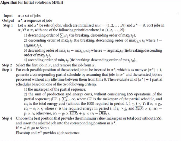
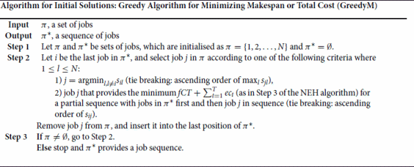
A chromosome in the GA is represented with a sequence of jobs, and a set of solutions (or chromosomes) is generated at the beginning. Three algorithms for initial solutions are proposed; (GreedyE) one considers energy consumption rates of jobs and assigns jobs spending a large amount of energy into the period with a small energy price; (MNEH) another applies the NEH algorithm, based on either makespan or the total cost without the ESS by considering sequence-dependent setup times; (GreedyM) the other selects the next job based on either the sequence-dependent setup times or the total cost without the ESS. Note that the proposed three algorithms are only used for determining a sequence of jobs, and they do not provide any assignment of jobs to periods or any energy schedule. The three algorithms are provided in detail.

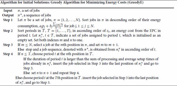
From the three algorithms, 11 chromosomes are obtained; the GreedyE algorithm generates one chromosome whereas the MNEH and GreedyM algorithms create eight and two chromosomes, respectively. In the GreedyE algorithm, jobs are sorted according to their energy consumption, $a_j{p}_j+b_j\frac{\sum _{i,i\ne j}{s}_{ij}}{N-1}$, with the assumption of the average setup time, $\frac{\sum _{i,i\ne j}{s}_{ij}}{N-1}$ of job j. Then the job with the largest energy usage is assigned to the period with the smallest energy price as long as the duration of the corresponding period is not fully occupied with jobs previously assigned. In a similar way, jobs are selected by following the descending order of their energy consumption and are assigned to periods in ascending order of the energy cost.

A modified NEH algorithm, called MNEH, sorts jobs according to one of four priorities based on sequence-dependent setup times as presented in Step 1; the sum of setup times, the maximum setup time, the difference between the maximum and second maximum setup times, and the minimum setup time. Then for each job selected based on one of the priorities, a partial schedule is derived by choosing the best position of the job based on either the makespan or the total cost without the ESS. The GreedyM algorithm selects a job that can minimise the setup time or the total cost without the ESS when it is positioned last in a partial sequence of jobs. An example of initial solutions, denoted as Example 2, is provided in the supplementary material.

The total number of 11 chromosomes are generated with the proposed three algorithms, and more chromosomes are generated randomly to have a given population size, $N_p$, which will be chosen between N and $2N$ through the preliminary experiments later. With $N_p$ chromosomes, idle times are determined, if needed, between jobs and energy schedules while minimising the total cost.

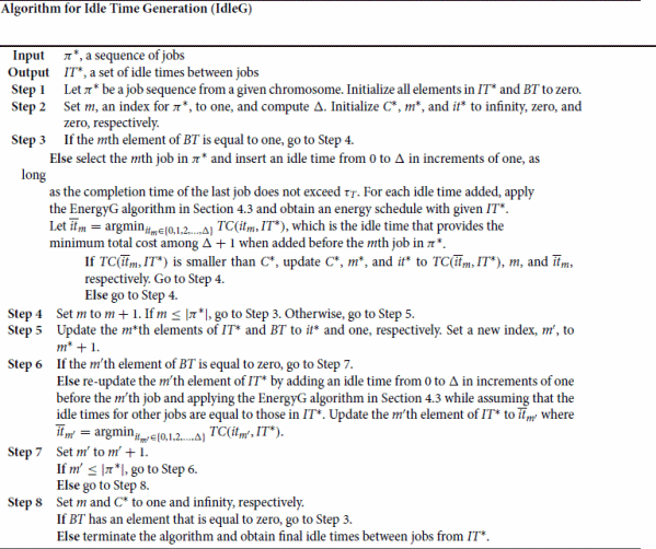
4.2. Idle time generation algorithm

In this subsection, an algorithm for adding idle times between jobs is proposed based on the sequence of jobs in a given chromosome, ${\pi }^{\ast }$. The basic idea of the algorithm is to compare the objective values by adding an idle time before each job from 0 to Δ, where $\mathrm{\Delta }=\underset{t\in \{1,\dots ,T\}}{max}{\mathrm{\Delta }}_t$, in increments of one (i.e. $0,1,\dots ,\mathrm{\Delta }$), and then to choose a certain idle time before the job that provides the minimum total cost among $(\mathrm{\Delta }+1)N$ schedules. Then, the algorithm adds the corresponding idle time before the job and further updates the idle times determined in the previous steps if it can decrease the objective value. Note that if adding an idle time only increases the total cost, the algorithm does not assign any idle time between jobs.

The total cost in the idle time generation algorithm indicates the objective value defined in Constraint (1), which includes not only the production cost but also the energy cost from the EPC, DER, and ESS. Hence, it requires an energy schedule whenever adding an idle time, and the algorithm for energy scheduling will be explained in the next subsection. Denote $I{T}^{\ast }$ as a set of idle times between the j−1th job and the jth job, $j\in {\pi }^{\ast }$, and BT as a set of binary values of N jobs in ${\pi }^{\ast }$, which indicates whether there is an idle time (> 0) before job j or not. Then $TC(i{t}_m,I{T}^{\ast })$ indicates an objective value obtained when adding an idle time as much as $i{t}_m$ before the mth job in ${\pi }^{\ast }$ with a given set, $I{T}^{\ast }$, for all the other jobs. Notations, $C^{\ast }$, $m^{\ast }$, and $i{t}^{\ast }$ in the algorithm, are used for indicating a minimum total cost obtained so far, the job before which an idle time is added, and an amount of idle time added, respectively. The following is the proposed idle time generation algorithm, IdleG algorithm, and an example of the algorithm, denoted as Example 3, is provided in the supplementary material.

4.3. Energy scheduling

Now, the energy scheduling algorithm is proposed to determine $C_t$, $D_t$ for the ESS, $D{U}_t$, $D{S}_t$ for the DER, and $E{U}_t$, $E{S}_t$ for the EPC. Then $TC(i{t}_m,I{T}^{\ast })$ in Steps 3 and 6 in the IdleG algorithm can be computed with Constraint (1). When a certain period, t, requires a high energy cost, $e_t$, it might be beneficial to store some energy into the ESS before period t if it is not expensive. Hence, the underlying idea of the energy scheduling algorithm is to compare $e_m$ and $g_m$ ($m<t$), and $e_t$ and $g_t$ and then store energy as much as possible to the ESS from the cheaper source, either from the EPC or DER in period m by considering the predetermined $C_m$ and $D_t$, $\overline{ESS}$, $\overline{EC}$, and $\overline{ED}$. However, if $e_t$ and $g_t$ are not expensive, the energy can be used directly from the EPC or DER in period t without using the ESS.

Let E be a set of energy prices in each period, $E=\{e_1,\dots ,e_T\}$, and G be a set of generation costs of the DER in each period, $G=\{g_1,\dots ,g_T\}$. $e_{\left(t\right)}$ and $g_{\left(t\right)}$ indicate the tth smallest energy cost in E and the tth smallest generation cost in G, respectively. EU is a set of amounts of energy directly used from the EPC in each period, $EU=\{E{U}_1,\dots ,E{U}_T\}$. In addition, $E{L}_{ml}$ is introduced, where $E{L}_{ml}=I_m+\underset{m\le k<l}{max}\left[\sum _{t=m}^k\right(C_t-D_t\left)\right]$, which represents the maximum level of energy stored in the ESS from period m to l−1 under a given energy charging/discharging schedule. It is used for computing the maximum available capacity of the ESS for charging in period m for later use in period l. The algorithm for energy scheduling, EnergyG, is explained as follows:

When a sequence of jobs and idle times between them are given, the algorithm first computes the required energy cost for each period in Step 1 without considering the ESS. In Step 2, the periods are sorted in non-decreasing order of the energy prices and generation costs. Then an energy schedule that determines amounts of energy used from the EPC or DER directly and used from the ESS by charging it in previous periods is determined from the period, denoted as l in Step 3, which has the largest total energy cost. Such energy schedules are derived by comparing the energy prices from the EPC and the generation costs from the ESS.

There are four cases in Step 4; First, when $e_{\left(k_e\right)}<g_{\left(k_g\right)}$ and $e_l<g_l$, it is beneficial to either charge the ESS from the EPC in period m for the energy usage in period l or use the energy directly from the EPC in period l depending on the energy prices in periods m and l. It is because the condition implies that the smallest energy price is less than the smallest generation cost and the energy price in period l is less than the generation cost in period l. Second, when $e_{\left(k_e\right)}<g_{\left(k_g\right)}$ and $e_l\ge g_l$, it might be good to charge the ESS from the EPC in period m or directly use it from the DER in period l. If $e_{\left(k_e\right)}\ge g_{\left(k_g\right)}$ and $e_l<g_l$, charging the ESS from the DER in period m or using the energy from the EPC in period l can be a good option. Finally, when $e_{\left(k_e\right)}\ge g_{\left(k_g\right)}$ and $e_l\ge g_l$, charging the ESS from the DER in period m or using the energy from the DER in period l is considered. The detailed explanation in Step 5 is as follows.

In Step 5-1, if $e_m+c+d<e_l$, which means that the sum of energy price in period m and the charging and discharging costs is less than the energy price in period l, an amount of energy, denoted as $A{C}_m$, is stored into the ESS in period m for using it in period l. $A{C}_m$ should be determined by considering the required energy in period l, $r_l$, the maximum charging capacity in period m, $\overline{EC}-C_m$, the maximum capacity of the ESS, $\text{β}\overline{ESS}-E{L}_{ml}$, and the maximum discharging capacity in period l, $\overline{ED}-D_l$. However, if $e_m+c+d\ge e_l$, the energy is supplied from the EPC directly in period l. Note that $r_l$ in Step 1 indicates the total energy required in period l, and it is updated to the remaining energy that needs to be further fulfilled in Steps 5-1 to 5-4. Based on the updated $r_l$, an amount of energy that needs to be stored in period m is determined. With the given sequence of jobs and idle times between jobs, the objective function of Constraint (1) can be obtained with the EnergyG algorithm.

In Step 5-2, if $e_m+c+d<g_l$, a certain amount of energy from the EPC is stored into the ESS in period m. However, if $e_m+c+d<e_l$, an amount of energy, as much as $min(r_l,{\overline{DER}}_l)$, from the DER is directly used in period l and the insufficient energy is supplied from the EPC in period m. Otherwise, the energy is supplied from the DER and EPC in period l without using the ESS.

In Step 5-3, if $g_m+c+d<e_l$, which means that the sum of the generation cost in period m and the charging and discharging costs is less than the energy price in period l, the energy from the DER is stored into the ESS in period m as much as $A{C}_m$ in Step 5-3. In this case, $A{C}_m$ is computed by considering $r_l$, ${\overline{DER}}_m$, $\overline{EC}-C_m$, $\text{β}\overline{ESS}-E{L}_{ml},$ and $\overline{ED}-D_l$. If $g_m+c+d\ge e_l$, the energy is directly used from the EPC in period l.

In Step 5-4, if $g_m+c+d<g_l$, it is better to charge energy from the DER into the ESS in period m for the usage in period l because the generation cost in period l is larger than that in period m. In this case, $A{C}_m$ is computed with $r_l$, ${\overline{DER}}_m$, $\overline{EC}-C_m$, $\text{β}\overline{ESS}-E{L}_{ml},$ and $\overline{ED}-D_l$ is stored into the ESS. If $g_m+c+d<e_l$, the energy from the DER in period l is used as much as $min(r_l,{\overline{DER}}_l)$ in period l, and then the insufficient energy is supplied from the ESS by charging it from DER in period m as much as $A{C}_m$. If $g_m+c+d\ge e_l$, the energy from the DER and EPC is used in period l.

For all periods in $\mathcal{T}$, Steps 4 to 6 are repeated, and the algorithm is terminated by finalising the energy schedule in Step 7. Note that the energy scheduling algorithm is applied in Steps 3 and 6 of the IdleG algorithm to determine an energy schedule and compute the total cost, $TC(i{t}_m,I{T}^{\ast })$, which includes ESS operations. The EnergyG algorithm stores a certain amount of energy in period m ($<l$) for period l. Therefore, the energy in period l cannot be used for the other periods ($>l$), which might decrease the efficiency of the algorithm.

An example of generating an energy schedule, denoted as Example 4, is provided in the supplementary material.

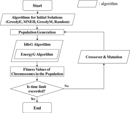
4.4. Overall procedure

An overall procedure of the proposed algorithm is illustrated in Figure 2. First, $N_p$ chromosomes, which consist of the first population, are generated; 11 chromosomes from the three algorithms (GreedyE, modified NEH, and GreedyM), and $N_p-11$ chromosomes from random generation (Random). Then the IdleG and EnergyG algorithms are applied to the population, and $N_p$ production and energy schedules are obtained. The fitness values of $N_p$ chromosomes in the population are then computed, and if the given time limit is not exceeded, the next population is generated through crossover and mutation operators applied to the current population.

Figure 2. An overall algorithm for energy-aware single-machine scheduling. An image that shows the overall algorithm for energy-aware single-machine scheduling consisting of ‘Algorithms for Initial Solutions’, ‘Population Generation’, ‘IdleG Algorithm’, ‘EnergyG Algorithm’, ‘Fitness Value Evaluation’, and ‘Crossover & Mutation’.

A pair of chromosomes, called parents, are selected from the current population and generate two new chromosomes, called children or offspring, with a crossover operator. $F_i$ denotes the fitness value of chromosome i, $1\le i\le N_p$, and a probability, $P_i^F$, $P_i^F=\frac{\frac{\sum _l{F}_l-F_i}{\sum _l{F}_l}}{N_p-1}$ to chromosome i, is assigned to $F_i$, so that the chromosome with a small fitness value can be chosen with a high probability when generating children. Then a one-point crossover, where a point is randomly chosen on both parents' chromosomes and genes to the right of the point are swapped between the two chromosomes, is used. The one-point crossover has been widely used in the GA for scheduling problems (Vallada and Ruiz 2011; Chung and Kim 2016; Joo and Kim 2015). Also, several studies showed that the one-point crossover provided a good performance compared to other operators (Ali Asghar et al. 2019; Hasançebi and Erbatur 2000). Note that if the set of jobs in each side of the crossover point is different, the jobs, which occur twice after the crossover operation, are changed randomly to other ones that do not appear in the chromosome so that it contains all jobs as genes.

A chromosome can be selected multiple times in one population to generate the offspring, and $2{\gamma }_c{N}_p$ chromosomes are newly generated through ${\gamma }_c{N}_p$ crossover operations where ${\gamma }_c$ is a hyper-parameter to determine the crossover ratio. After that, a mutation operator that swaps two genes randomly in a child's chromosome is applied with the probability of ${\gamma }_m$.

Then $N_p$ chromosomes among $N_p+2{\gamma }_c{N}_p$ chromosomes ($N_p$ original chromosomes and $2{\gamma }_c{N}_p$ new chromosomes after the crossover and mutation operations) are selected with an elitism policy that chooses ${\gamma }_e{N}_p$ chromosomes with small fitness values and $N_p-{\gamma }_e{N}_p$ chromosomes based on $P_i^F$, $1\le i\le N_p+2{\gamma }_c{N}_p-{\gamma }_e{N}_p$. Then a new set of population is composed, and the proposed algorithm is repeated until the time limit. Note that the selected chromosomes might be similar to ones chosen only with the small fitness values but sill can be different due to the probability feature of $P_i^F$.

5. Experimental results

The experiments of the proposed algorithm is performed for energy-aware single-machine scheduling with the DER and ESS to minimise the sum of production and energy costs. The algorithm is coded with JAVA programming language and run on a personal computer with Intel Core i7-9700 and 32 GB RAM. An optimal solution with the proposed mathematical model is obtained with GUROBI (Version 9.1.0).

5.1. Preliminary experiments

When N and T were larger than 20 and 12, respectively, there were some instances where GUROBI was not able to provide an optimal solution within an hour. Hence, N and T are set to 15 and 12, respectively, for determining hyper-parameters by comparing the objective value from the hybrid GA to an optimal solution from GUROBI. ${\mathrm{\Delta }}_t$ is 60 minutes for all t, and $p_j$ and $s_{ij}$ are randomly generated from the Uniform distribution U(25, 45) and U(1, 5), respectively, by considering the period, 720 minutes. The time unit is a minute. $a_j$ is also randomly generated between 3 and 6 kW per minute, and $b_j$ is set to $a_j-1$. $\overline{EC}$ is equal to $\overline{ED}$ and determined between 50 and 100 kW randomly. c and d are set to 10 KRW/kW, and $\overline{ESS}$ is 300 kW with α of 0.2 and β of 0.9. $e_t$ follows the ToU pricing during the summer in Table 1 by averaging the prices of the consecutive two hours so that 12 periods can be obtained. Hence, $e_t$, $1\le t\le 12$, is set to 56.1, 56.1, 56.1, 56.1, 82.55, 191.1, 150.1, 191.1, 50.1, 109, 109, and 82.55 KRW/kW starting from the midnight. $g_t$ is determined to be 60 KRW/kW for all t. ${\overline{DER}}_t$, $1\le t\le 12$, is selected from the Normal distribution, $N(\mu ,\sigma )$, which is determined from the real data of the factory considered. $N(\mu ,\sigma )$ for period t, $1\le t\le 12$, is set to be $N(0,0)$, $N(0,0)$, $N(0,0)$, $N(0,0)$, $N(21.3,10.9)$, $N\left(97.320.2\right)$, $N(133.2,29.8)$, $N(144.5,34.2)$, $N(129.1,29.1)$, $N(64.9,22.7)$, $N(5.38,4.2)$, and $N(0,0)$. The parameters used for the experiments have been selected from the previous studies and the factory we considered. The processing times, setup times, $\overline{ESS}$, and ${\overline{DER}}_t$ have been determined by considering the planning horizon and the real data of the factory. $a_j$ and $b_j$ have been selected from the machine energy consumption per hour in previous works (Moon, Shin, and Park 2013; Moon and Park 2014; Che, Zeng, and Lyu 2016). $g_t$, c, and d have been chosen to reflect the proportion of the DER and ESS costs to the total energy in practice. The computation time limit of the proposed algorithm is set to 10 minutes. The production and energy cost changes are provided depending on the parameters.

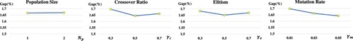
The hyper-parameters, $N_p\in \left\{1\right(=N),2(=2N\left)\right\}$, ${\gamma }_c\in \{0.5,0.7,0.9\}$, ${\gamma }_e\in \{0.5,0.7,0.9\}$, and ${\gamma }_m\in$ $\{0.01,0.03,0.05\}$, are tested with f of 10 and 200 KRW/min to see the impact of the ratio of the production cost to energy cost on the performance of the algorithm. The production cost accounts for about 4-5 % and 35-40 % with f of 10 and 200 in the total cost, respectively. The cost from the ESS and DER mostly accounts for 10 % in the total cost. 10 instances are randomly generated for each parameter set, and the average objective value from running five times of the hybrid GA for one instance is compared to an optimal solution from GUROBI. Figure 3 shows the average gap, computed by $\frac{(\mathrm{o}\mathrm{b}\mathrm{j}\mathrm{e}\mathrm{c}\mathrm{t}\mathrm{i}\mathrm{v}\mathrm{e}\mathrm{f}\mathrm{r}\mathrm{o}\mathrm{m}\mathrm{t}\mathrm{h}\mathrm{e}\mathrm{p}\mathrm{r}\mathrm{o}\mathrm{p}\mathrm{o}\mathrm{s}\mathrm{e}\mathrm{d}\mathrm{a}\mathrm{l}\mathrm{g}\mathrm{o}\mathrm{r}\mathrm{i}\mathrm{t}\mathrm{h}\mathrm{m}-\mathrm{o}\mathrm{p}\mathrm{t}\mathrm{i}\mathrm{m}\mathrm{a}\mathrm{l}\mathrm{s}\mathrm{o}\mathrm{l}\mathrm{u}\mathrm{t}\mathrm{i}\mathrm{o}\mathrm{n})\times 100}{\mathrm{o}\mathrm{p}\mathrm{t}\mathrm{i}\mathrm{m}\mathrm{a}\mathrm{l}\mathrm{s}\mathrm{o}\mathrm{l}\mathrm{u}\mathrm{t}\mathrm{i}\mathrm{o}\mathrm{n}}$, with f of 10 for each hyper-parameter set. The average gap over all hyper-parameter sets is 1.67 % with f of 10, and it is 1.06 % with f of 200. As can be seen in Figure 3, a small gap is usually obtained with $N_p$ of 1, ${\gamma }_c$ of 0.5, ${\gamma }_e$ of 0.5, and ${\gamma }_m$ of 0.05. A similar pattern is found from the results with f of 200. Note that ${\gamma }_m$ of 0.1, 0.2, and 0.3 was tested, but there was no significant difference in the gap. The average computation time of GUROBI is 1608 s and 724 s with f of 10 and 200, respectively. Hereafter, those parameter values are used to evaluate the performance of the algorithm further.

Figure 3. Preliminary experiments for setting parameters. Four graphs of preliminary experiments for parameter setting that show gaps according to population size, crossover ratio, elitism, and mutation rate, respectively.

5.2. Comparison to optimal solutions

As can be seen in the preliminary experiments, the average gaps are less than 2 % with N of 15, which is very small. N is increased to 20, 25, and 30, each of which has $p_j$ randomly determined from U(20, 30), U(15, 25), U(10, 20), respectively, with T of 12. $s_{ij}$ is randomly generated from U(1, 3) (setup type 1) or U(1, 5) (setup type 2), to see the impact of setup time ranges, and $g_t$ is set to 40 or 60 KRW/kW for all t to analyse the impact of the generation cost. All the other parameters are the same as in the preliminary experiments. The proposed GA is run for 10 minutes. Note that the number of jobs has been determined to show the efficiency of the proposed algorithm by comparing it to optimal solutions. GUROBI is able to provide optimal solutions for some instances with 20 jobs and no optimal solutions for 25 and 30 jobs within an hour, which will be shown in Table 2. In addition, the factory we consider produces 25 to 50 jobs on average in a half day.

Table 2. Comparison between GUROBI and hybrid GA.

N	f	$g_t$	ST	Avg. Gap (%)	Std. Gap	hGa Std./Avg. (%)	PR(GRB)	PR(hGA)	PC(GRB/hGA)	EC(GRB/hGA)	GRB Comp. Time	NI_Optimal	NI_Initial
20	10	40	1	3.67	0.87	0.53	4.49	4.49	0.96	0.96	3041.90	21	0
	10	40	2	4.45	0.95	0.63	4.61	4.52	0.97	0.96	3364.70	25	0
	10	60	1	2.01	0.44	0.44	4.20	4.16	0.99	0.98	3068.47	18	1
	10	60	2	1.98	0.85	0.47	4.32	4.20	1.01	0.98	3501.89	25	0
	200	40	1	2.78	0.95	0.35	42.04	40.25	1.02	0.94	2841.95	13	0
	200	40	2	3.62	1.22	0.56	42.61	40.75	1.01	0.94	3306.15	24	0
	200	60	1	1.32	0.48	0.29	40.74	40.60	0.99	0.98	3165.34	16	0
	200	60	2	1.33	0.34	0.48	41.34	40.78	1.00	0.98	3386.46	25	0
	Avg.			2.65	0.76	0.47	−	−	0.99	0.97	3209.61	20.88	0.13
25	10	40	1	4.39	1.52	0.59	4.59	4.63	0.93	0.94	3600.00	30	12
	10	40	2	4.56	1.19	0.66	4.72	4.71	0.96	0.96	3600.00	30	2
	10	60	1	1.76	1.29	0.47	4.47	4.53	0.97	0.98	3600.00	30	6
	10	60	2	1.73	1.68	0.61	4.33	4.41	0.97	0.98	3600.00	30	0
	200	40	1	3.85	1.30	0.46	43.03	40.74	1.02	0.93	3600.00	30	2
	200	40	2	4.17	1.78	0.72	42.58	40.38	1.01	0.92	3600.00	30	2
	200	60	1	0.57	1.00	0.46	40.81	40.72	1.00	0.99	3600.00	30	6
	200	60	2	1.93	0.99	0.63	41.20	40.53	1.00	0.97	3600.00	30	0
	Avg.			2.87	1.34	0.58	−	−	0.98	0.96	3600.00	30	3.75
30	10	40	1	3.79	1.43	0.79	5.25	5.06	0.99	0.96	3600.00	30	20
	10	40	2	2.94	3.23	1.02	4.49	4.82	0.96	0.97	3600.00	30	14
	10	60	1	0.96	0.56	0.60	4.72	4.61	1.00	0.99	3600.00	30	24
	10	60	2	0.46	1.81	0.90	4.68	4.59	1.02	0.99	3600.00	30	10
	200	40	1	3.56	0.41	0.59	43.86	42.75	0.98	0.95	3600.00	30	20
	200	40	2	4.08	1.46	0.83	43.63	41.97	0.99	0.94	3600.00	30	18
	200	60	1	$-0.34$	2.30	0.54	41.28	41.82	1.00	1.00	3600.00	30	22
	200	60	2	1.08	0.58	0.99	41.52	41.92	0.93	0.98	3600.00	30	24
	Avg.			2.07	1.47	0.78	−	−	0.98	0.97	3600.00	30	19

Table 2 shows the results according to N, f, $g_t$, and setup types (ST). 30 instances were generated for each problem, and the proposed hybrid GA was run 30 times for each instance. Then the average of 30 results is compared to the total cost from GUROBI with a time limit of 3600 s. Denote TC${}_{GRB}$ and TC${}_{hGA}$ as the total cost (the objective value) from GUROBI and the proposed hybrid GA, respectively. PC${}_{GRB}$ (EC${}_{GRB}$) and PC${}_{hGA}$ (EC${}_{hGA}$) indicate the production (energy) cost from GUROBI and the proposed algorithm, respectively. The average gap in the fifth column of Table 2 is computed by (TC${}_{hGA}$ - TC${}_{GRB}$)× 100/TC${}_{GRB}$, and the standard deviation of the gaps from 30 instances is presented in the sixth column. The seventh column shows the average value of ‘standard deviation of the total cost×100/total cost’ from the proposed hybrid GA. The eighth and ninth columns, PR(GRB) and PR(hGA) in Table 2, show the production cost ratios, which are computed as PC${}_{GRB}$/TC${}_{GRB}$ and PC${}_{hGA}$/TC${}_{hGA}$, respectively. The production and energy costs are compared from GUROBI and our algorithm with PC(GRB/hGA) and EC(GRB/hGA), which are computed by PC${}_{GRB}$/PC${}_{hGA}$ and EC${}_{GRB}$/EC${}_{hGA}$, respectively. The average computation time of GUROBI by setting 3600 s for instances where optimal solutions are not found within an hour is represented in the twelfth column. The last two columns show the number of instances where optimal solutions were not found (NI_Optimal) and where even an initial solution was not found (NI_Initial) within an hour from GUROBI, respectively. The gaps were computed only for instances where initial solutions were found within an hour. Figure 4 shows the results from Table 2 for each of 20, 25, and 30 jobs. The x-axis indicates the combination of $f/g_t/ST$, and the y-axis is the average gap in Figure 4.

Figure 4. Summary of comparison with 20, 25, and 30 jobs. A graph that shows the summary of comparison for 20, 25, and 30 jobs with various combinations of f, $g_t$, and ST.

It is observed in Table 2 that GUROBI was not able to find an optimal solution within an hour for all instances with 25 and 30 jobs from NI_Optimal. In addition, it did not even provide any solution with 30 jobs for the average of 19 instances of each problem, and such cases were excluded in computing the gap between the algorithm and GUROBI. It is worth noting that the average optimality gap of GUROBI, which is obtained when optimal solutions are not found within an hour, is 0.85, 2.21, and 3.77 % for 20, 25, and 30 jobs, respectively. Note that the performance evaluation of the hybrid GA for large-sized problems by relaxing the problem was not successful because the proposed mathematical model even without the subtour elimination constraint, Constraint (18), did not provide any feasible solution within an hour for 15 instances among 30 instances of 30 jobs on average.

In Table 2, the average gaps with 20, 25, and 30 jobs between our algorithm and GUROBI are 2.65, 2.87, and 2.07 %, respectively. There is no significant impact of the setup times on the average gaps. The results of 30 jobs in Table 2 should be used just for reference because most of the instances were not solved by GUROBI within an hour.

In Table 2 and Figure 4, it can be observed that the average gaps with $g_t$ of 40 are larger than those with $g_t$ of 60 in general. When $g_t$ is 40, generating the energy from the DER can be efficient than buying it from the EPC because the minimum $e_t$ is 56.1. Hence, the energy scheduling for the ESS, DER, and EPC affects the performance more than the production schedule in this case. It is also observed that EC(GRB/hGA) in Table 2 is smaller with $g_t$ of 40 than that with $g_t$ of 60, which means that EC${}_{hGA}$ becomes closer to EC${}_{GRB}$ in the case. The overall average gap and standard deviation of the gap for all jobs are 2.53 % and 1.19, respectively. The ratio of the standard deviation of the total cost to the total cost for all jobs is 0.61 %. The Wilcoxon signed-rank test with the total costs from the proposed algorithm and GUROBI for each parameter set in Table 2 (total 24 sets) has been conducted. The p values for 23 sets were larger than 0.05, and only one of them (25 jobs, f of 200, $g_t$ of 40, ST of 2) had the p value of 0.01. Therefore, it can be observed that there is no statistically significant difference between the total costs from the hybrid GA and GUROBI in most instances. The minimum total cost changes in each iteration of the proposed algorithm for an instance of 20, 25, and 30 jobs are presented in the supplementary material.

From Table 2 and Figure 4, it can be seen that $g_t$ affects the average gap more than other parameters. We have further performed the experiments with $g_t$ of 60 and 80, but the average gaps between $g_t$ of 20 and 40 and between $g_t$ of 60 and 80 were similar. Note that there is also no large difference even with a large f($>200$).

5.3. Performance of the algorithm

The effectiveness of adding intentional idle times between jobs is evaluated by running the hybrid GA with and without the IdleG algorithm. Table 3 shows the cost ratio (cost from GA with IdleG/cost from GA without IdleG) for all elements in the total cost, which are the production cost, EPC cost, ESS cost, DER cost, as well as the total cost, with 20 jobs. Figure 5 shows the ratio graphs in Table 3. Note that the ratios are similar regardless of the number of jobs. It can be seen that the production cost is larger with the IdleG algorithm because idle times between jobs are added, but the EPC cost is smaller by delaying some jobs and using the DER and ESS efficiently. The IdleG algorithm significantly reduces the EPC cost when f is 10, which results in approximate 10 % reduction in the total cost. The ESS cost ratio is increased whereas the DER cost ratio is decreased as $g_t$ is changed from 40 to 60 as can be seen in Figure 5. This is because it can be better to use less energy from the DER and to use the ESS more frequently by saving energy from the EPC when $g_t$ is high. There is no large difference between setup types. When f is 200, most cost ratios are close to 1 because it is better to reduce idle times between jobs to minimise the production cost.

Figure 5. Evaluation of the IdleG algorithm. A graph that shows the impact of IdleG algorithm on the total cost, production cost, EPC cost, ESS cost, and DER cost with various combinations of f, $g_t$, and ST.

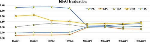
Table 3. Comparison of the hybrid GA with and without the IdleG algorithm with 20 jobs.

f	$g_t$	ST	PC	EPC Cost	ESS Cost	DER Cost	TC
10	40	1	1.36	0.85	1.00	1.20	0.89
10	40	2	1.37	0.86	1.04	1.22	0.90
10	60	1	1.37	0.86	1.07	1.12	0.90
10	60	2	1.35	0.86	1.05	1.10	0.90
200	40	1	1.01	0.99	1.00	1.06	1.01
200	40	2	1.02	1.00	1.00	1.07	1.01
200	60	1	1.04	0.96	1.00	1.06	1.00
200	60	2	1.05	0.96	1.02	1.08	1.01

The final experiments are performed to see how much cost can be saved by having the ESS and DER. This analysis can be conducted with the proposed algorithm. N is set to 50 and 100, and T is set to 24 (one day, 1440 minutes) by reflecting the real factory schedule. $p_j$ and $s_{ij}$ are randomly generated from U(15, 25) and U(1, 3) and from U(7, 12) and U(1, 2), respectively, for 50 and 100 jobs. The energy price during the summer in Table 1 is used. All the other parameters are the same with the previous experiments. 30 instances for each parameter set (f and $g_t$) are generated with and without the ESS, DER and both of the ESS and DER. Then, the production cost, energy cost and total cost ratios are compared for three cases, with/without ESS, with/without DER, and with/without both.

In Table 4, the average ratio of the total cost for each case is 0.98, 0.83, and 0.80, respectively. When there is no ESS, the energy from the EPC and DER is directly used without storage, and hence, delaying some jobs may not provide good solutions. Hence, the production cost ratio is larger than 1 with f of 10. It is less than 1 when f becomes 200. If an ESS is used, some energy during inexpensive periods can be stored and used when the energy price is high. Therefore, if f is large, not delaying some jobs even during expensive periods can be beneficial with the ESS. However, if there is no ESS, it might be necessary to delay some jobs when the energy price is high. If there is no DER, all energy from the EPC needs to be used directly or to be stored in the ESS. The average energy cost ratio in the second case (with/without DER) is 0.81, which means that the energy cost can be saved as much as 19 % with the DER. When both of the ESS and DER are used, the average energy cost is reduced to 0.79. This cost saving comes from one day production, and it can be much larger when the period extends to a week and a month. Figure 6 shows the total cost of the schedules with and without both of the ESS and DER (wB, w/oB) depending on the number of jobs, f and $g_t$ (i.e. x-axis indicates N/f/$g_t$). When f is 200, the average production cost and energy cost are increased by 18 % and 26 %, respectively, on average, compared to the case with the ESS and DER. Note that the amount of costs that can be saved by having the ESS and DER depends on the ESS capacity, ESS operating cost, DER maximum capacity, and DER generation cost. Companies that are considering to have a DER or ESS can use the proposed algorithm for analysing their effectiveness.

Figure 6. Comparison of schedules with and without ESS and DER. A graph that shows the impact of ESS and DER on the total cost with various combinations of N, f, and $g_t$.

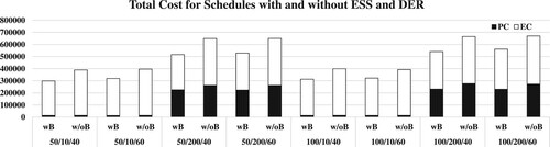
Table 4. Total cost analysis without ESS and DER.

			with/without ESS			with/without DER			with/without Both
N	f	$g_t$	PC	EC	TC	PC	EC	TC	PC	EC	TC
50	10	40	1.10	0.98	0.99	0.98	0.78	0.78	0.97	0.76	0.77
	10	60	1.03	0.97	0.97	0.92	0.83	0.83	0.92	0.80	0.81
	200	40	0.96	1.01	0.99	0.88	0.78	0.82	0.86	0.75	0.80
	200	60	0.95	0.99	0.97	0.90	0.80	0.84	0.85	0.79	0.81
100	10	40	1.06	0.99	0.99	0.94	0.80	0.81	0.94	0.78	0.78
	10	60	1.06	0.95	0.96	0.93	0.84	0.84	0.93	0.82	0.82
	200	40	0.96	1.00	0.98	0.88	0.80	0.83	0.84	0.80	0.81
	200	60	0.95	0.99	0.97	0.91	0.83	0.86	0.85	0.83	0.84

6. Conclusion

A single-machine scheduling problem has been addressed, where processing and setups of jobs require a certain amount of energy, the energy can be obtained from the EPC and DER, and it can be stored in the ESS, with the objective of minimising the sum of production and energy costs. The mathematical programming model has been developed first, and then the hybrid GA has been proposed. The proposed algorithm consists of initial solution methods, the idle time generation algorithm which adds appropriate idle times between jobs by considering the total cost, and the energy scheduling algorithm that determines the energy usage from the EPC, DER, and ESS. The proposed algorithm has been evaluated with optimal solutions from GUROBI under various scenarios, and the gap was less than 3 % on average. The efficiency of the IdleG algorithm and of having the ESS and DER has been evaluated.

This research can be further extended by considering other manufacturing environments, such as parallel machines, flow shops or job shops. The different energy consumption of machines (unrelated or uniform parallel machines) can also be considered. In addition, the cost reduction with the DER and ESS may need to be further analysed to determine an appropriate capacity of the DER and ESS. Other methods, such as a reinforcement learning approach to determine idle times between jobs or a sequence of jobs, can be applied. Applying the advanced meta-heuristics, such as PSO, ABC, GSA, and GWO, by considering the DER and ESS can also be good future work.

Disclosure statement

No potential conflict of interest was reported by the author(s).

Data Availability Statement

The data that support the findings of this study is available from the corresponding author, Jun-Ho Lee, upon reasonable request.

Additional information

Funding

This work was supported by the National Research Foundation of Korea Grant funded by the Korean Government [grant number NRF-2019S1A2A2031006].

Notes on contributors

Hyun-Jung Kim

Hyun-Jung Kim received the Ph.D. degree in Industrial and Systems Engineering from KAIST (Korea Advanced Institute of Science and Technology), Daejeon, Republic of Korea in 2013. She was a Postdoctoral Researcher in the Department of Industrial Engineering & Operations Research, University of California, Berkeley, and was an Assistant Professor in the Department of Systems Management Engineering, Sungkyunkwan University, Republic of Korea. She is now an Assistant Professor with the Department of Industrial & Systems Engineering, KAIST. Her research interests include modelling, scheduling, and control of production systems.

Eun-Seok Kim

Eun-Seok Kim is an Associate Professor in Operations Management at Queen Mary, University of London, United Kingdom. He has BSc, MSc and PhD degrees in Operational Research from KAIST (Korea Advanced Institute of Science and Technology), South Korea. Before joining Queen Mary, he was an Assistant/Associate Professor in Operations Management and Programme Leader in MSc Global Supply Chain Management at Middlesex University, United Kingdom. His main research interest falls within the field of operations and supply chain management specialising in combinatorial optimisation and scheduling theory. He is also interested in applications of operational research, especially optimisation, to various problem areas including telecommunication and actuarial science.

Jun-Ho Lee

Jun-Ho Lee received the B.S. and Ph.D. degrees from the Department of Industrial and Systems Engineering, KAIST (Korea Advanced Institute of Science and Technology), Daejeon, Republic of Korea, in 2008 and 2013, respectively. He was a Senior Researcher at Systems Engineering Team, Samsung Electronics, Republic of Korea, from 2013 to 2016, and was a Postdoctoral Researcher at the Department of Industrial and Systems Engineering, University of Wisconsin, Madison, WI, USA, from 2016 to 2017. He is currently an Assistant Professor with the School of Business, Chungnam National University, Republic of Korea. His research interests are in modelling, analysis, scheduling, and control of production and service systems.

Lixin Tang

Lixin Tang received the B.Eng. degree in industrial automation, the M.Eng. degree in systems engineering and the Ph.D. degree in control science and engineering from Northeastern University, Shenyang, China, in 1988, 1991, 1996, respectively. He is a member of Chinese Academy of Engineering, the Director of Key Laboratory of Data Analytics and Optimization for Smart Industry, Ministry of Education, China, and the Chair Professor of Centre for Industrial Intelligence and Systems Optimization, Northeastern University. His research interests cover industrial intelligence and systems optimisation theories and methods, including data analytics and machine learning, deep learning and evolutionary learning, reinforcement learning and dynamic optimisation, convex and sparse optimisation, integer and combinatorial optimisation, computational intelligence-based optimisation. Meanwhile, he applies the above theories to engineering applications in manufacturing, logistics and energy systems. He has published many papers in international journals such as Operations Research, Manufacturing & Service Operations Management, INFORMS Journal on Computing, IISE Transactions, Naval Research Logistics, et al. His paper published on IISE Transactions received the Best Applications Paper Award of 2017. He currently serves as an Associate Editor of IISE Transactions, IEEE Transactions on Evolutionary Computation, IEEE Transactions on Cybernetics, Journal of Scheduling, International Journal of Production Research, and Journal of the Operational Research Society. Meanwhile, he is on the Editorial Board of Annals of Operations Research, and serves as an Area Editor of the Asia-Pacific Journal of Operational Research.

Yang Yang

Yang Yang received the B.S. degree in automation from Northeastern University, Shenyang, China, and the Ph.D. degree in systems engineering from Northeastern University, Shenyang, China, in 2003 and 2010, respectively. She is currently an Associate Professor with Centre for Industrial Intelligence and Systems Optimization, Northeastern University. Her current research interests include production planning and scheduling, integer and combinatorial optimisation and engineering applications in manufacturing systems.

References

- Aghelinejad, M., Y. Ouazene, and A. Yalaoui. 2018. “Production Scheduling Optimisation with Machine State and Time-dependent Energy Costs.” International Journal of Production Research 56 (16): 5558–5575.
- Ali Asghar, R. H., V. Javad, S. Behzad, S. Arun Kumar, and E. Mohaned. 2019. “Extended Genetic Algorithm for Solving Open-shop Scheduling Problem.” Soft Computing 23: 5099–5116.
- Araceli, F.-P., L. Peter, and V. Tiffany. 2019. “Industry: Tracking Clean Energy Progress”. https://www.iea.org/tcep/industry/.
- Che, A., Y. Zeng, and K. Lyu. 2016. “An Efficient Greedy Insertion Heuristic for Energy-conscious Single Machine Scheduling Problem Under Time-of-Use Electricity Tariffs.” Journal of Cleaner Production 129: 565–577.
- Che, A., S. Zhang, and X. Wu. 2017. “Energy-conscious Unrelated Parallel Machine Scheduling Under Time-of-use Electricity Tariffs.” Journal of Cleaner Production 156: 688–697.
- Cheng, J., F. Chu, and M. Zhou. 2018. “An Improved Model for Parallel Machine Scheduling Under Time-of-use Electricity Price.” IEEE Transactions on Automation Science and Engineering 15 (2): 896–899.
- Chung, B. D., and B. S. Kim. 2016. “A Hybrid Genetic Algorithm with Two-stage Dispatching Heuristic for a Machine Scheduling Problem with Step-deteriorating Jobs and Rate-modifying Activities.” Computers & Industrial Engineering 98: 113–124.
- Ding, J.-Y., S. Song, R. Zhang, R. Chiong, and C. Wu. 2016. “Parallel Machine Scheduling Under Time-of-use Electricity Prices: New Models and Optimization Approaches.” IEEE Transactions on Automation Science and Engineering 13 (2): 1138–1154.
- Gahm, C., F. Denz, M. Dirr, and A. Tuma. 2016. “Energy-Efficient Scheduling in Manufacturing Companies: A Review and Research Framework.” European Journal of Operational Research 248 (3): 744–757.
- Gao, K., Y. Huang, A. Sadollah, and L. Wang. 2020. “A Review of Energy-efficient Scheduling in Intelligent Production Systems.” Complex & Intelligent Systems 6: 237–249.
- Gong, X., T. D. Pessemier, W. Joseph, and L. Martens. 2015. “An Energy-Cost-Aware Scheduling Methodology for Sustainable Manufacturing.” Procedia CIRP 29: 185–190.
- Hasançebi, O., and F. Erbatur. 2000. “Evaluation of Crossover Techniques in Genetic Algorithm Based Optimum Structural Design.” Computers and Structures 78: 435–448.
- Joo, C. M., and B. S. Kim. 2015. “Hybrid Genetic Algorithms with Dispatching Rules for Unrelated Parallel Machine Scheduling with Setup Time and Productivity Availability.” Computers & Industrial Engineering 85: 102–109.
- Lee, Y. H., K. Bhaskaran, and M. Pinedo. 1997. “A Heuristic to Minimize the Total Weighted Tardiness with Sequence-dependent Setups.” IIE Transactions 29 (1): 45–52.
- Liao, C.-J., and H.-C. Juan. 2007. “An Ant Colony Optimization for Single-Machine Tardiness Scheduling with Sequence-dependent Setups.” Computers & Operations Research 34 (7): 1899–1909.
- Liu, Y., H. Dong, N. Lohse, and S. Petrovic. 2016. “A Multi-objective Genetic Algorithm for Optimisation of Energy Consumption and Shop Floor Production Performance.” International Journal of Production Economics 179: 256–272.
- Luo, S., L. Zhang, and F. Yushun. 2019. “Energy-efficient Scheduling for Multi-objective Flexible Job Shops with Variable Processing Speeds by Grey Wolf Optimization.” Journal of Cleaner Production234: 1365–1384.
- May, G., B. Stahl, M. Taisch, and V. Prabhu. 2015. “Multi-objective Genetic Algorithm for Energy-Efficient Job Shop Scheduling.” International Journal of Production Research 53 (23): 7071–7089.
- Merkerts, L., L. Harjunkoski, A. Lsaksson, S. Säynevirta, A. Saarela, and G. Sand. 2015. “Scheduling and Energy – Industrial Challenges and Opportunities.” Computers & Chemical Engineering 72 (2): 183–198.
- Moon, J.-Y., and J. Park. 2014. “Smart Production Scheduling with Time-dependent and Machine-dependent Electricity Cost by Considering Distributed Energy Resources and Energy Storage.” International Journal of Production Research 52 (13): 3922–3939.
- Moon, J.-Y., K. Shin, and J. Park. 2013. “Optimization of Production Scheduling with Time-dependent and Machine-dependent Electricity Cost for Industrial Energy Efficiency.” The International Journal of Advanced Manufacturing Technology 68 (1): 523–535.
- Mustu, S., and E. Tamer. 2018. “The Single Machine Scheduling Problem with Sequence-dependent Setup Times and a Learning Effect on Processing Times.” Applied Soft Computing 71: 291–306.
- OECD-IEA. 2019, “CO2 Emissions from Fuel Combustion 2019”, Statistics Report.
- Ovacikt, I. M., and R. Uzsoy. 1994. “Rolling Horizon Algorithms for a Single-machine Dynamic Scheduling Problem with Sequence-dependent Setup Times.” International Journal of Production Research 32 (6): 1243–1263.
- Pinedo, M. L.. 2012. Scheduling Theory, Algorithms, and Systems. New York, NY, USA: Springer.
- Rahimifard, S., Y. Seow, and T. Childs. 2010. “Minimising Embodied Product Energy to Support Energy Efficient Manufacturing.” CIRP Annals – Manufacturing Technology 59 (1): 25–28.
- Rubaiee, S., and M. B. Yildirim. 2019. “An Energy-aware Multiobjective Ant Colony Algorithm to Minimize Total Completion Time and Energy Cost on a Single-Machine Preemptive Scheduling.” Computers & Industrial Engineering 127: 240–252.
- Salonitis, K., M. R. Jolly, B. Zeng, and H. Mehrabi. 2016. “Improvements in Energy Consumption and Environmental Impact by Novel Single Shot Melting Process for Casting.” Journal of Cleaner Production 137 (20): 1532–1542.
- Shrouf, F., J. Ordieres-Meré, A. García-Sánchez, and M. Ortega-Mier. 2014. “Optimizing the Production Scheduling of a Single Machine to Minimize Total Energy Consumption Costs.” Journal of Cleaner Production 67 (15): 197–207.
- Tang, D., M. Dai, M. A. Salido, and A. Giret. 2016. “Energy-efficient Dynamic Scheduling for a Flexible Flow Shop Using An Improved Particle Swarm Optimization.” Computers in Industry 81: 82–95.
- UN Sustainable Development. 2020. https://www.un.org/sustainabledevelopment/energy/.
- Vallada, E., and R. Ruiz. 2011. “A Genetic Algorithm for the Unrelated Parallel Machine Scheduling Problem with Sequence Dependent Setup Times.” European Journal of Operational Research 211 (3): 612–622.
- Vélez-Gallego, M. C., J. Maya, and J. R. Montoya-Torres. 2016. “A Beam Search Heuristic for Scheduling a Single Machine with Release Dates and Sequence Dependent Setup Times to Minimize the Makespan.” Computers & Operations Research 73: 132–140.
- Wang, C., C. Liu, Z.-H. Zhang, and L. Zheng. 2016. “Minimizing the Total Completion Time for Parallel Machine Scheduling with Job Splitting and Learning.” Computers & Industrial Engineering 97: 170–182.
- Yildirim, M. B., and G. Mouzon. 2012. “Single-Machine Sustainable Production Planning to Minimize Total Energy Consumption and Total Completion Time Using a Multiple Objective Genetic Algorithm.” IEEE Transactions on Engineering Management 59 (4): 585–597.
- Zhang, R., and R. Chiong. 2016. “Solving the Energy-efficient Job Shop Scheduling Problem: a Multi-objective Genetic Algorithm with Enhanced Local Search for Minimizing the Total Weighted Tardiness and Total Energy Consumption.” Journal of Cleaner Production 112: 3361–3375.
- Zhu, X., and W. E. Wilhelm. 2006. “Scheduling and Lot Sizing with Sequence-dependent Setup: A Literature Review.” IIE Transactions 38: 987–1007.