Optimising the fermentation throughput in biomanufacturing with bleed–feed

Abstract

Bleed–feed is a novel technology that allows biomanufacturers to skip bioreactor setups. However, the time at which bleed–feed is performed is important for its successful implementation. In addition, bleed–feed operations involve unique trade-offs that affect the system's throughput. For example, the biomass replenishment amount during bleed–feed affects the expected yield of the system. In this study, we formalise these operational trade-offs and formulate a stochastic optimisation model using renewal reward theory. Our analytical model captures both the biological dynamics and operational trade-offs of bleed–feed decisions to maximise throughput. We present an industry case study to demonstrate the use of our model. Through several practically relevant scenarios, we assess the potential impact of implementing bleed–feed on current practice and develop insights for practitioners. Although our work is primarily motivated by the biomanufacturing industry, our analytical model and insights are applicable to other industries that involve fermentation. Our results show that bleed–feed brings the most benefit for fast-growing cells or high-risk cultures. Although counter-intuitive, our numerical analysis shows that it is optimal not to adopt bleed–feed when biomass accumulation is too slow.

Keywords:

• Biomanufacturing
• fermentation
• bleed–feed
• renewal theory
• stochastic modelling

1. Introduction

The biomanufacturing industry introduced several new drugs (known as biopharmaceuticals) to treat diseases and provide better healthcare services. Thanks to these biopharmaceuticals, more than 345 million patients worldwide survived from cardiovascular diseases, cancer, diabetes and many others. The growing number of geriatric population and surge in preventing chronic diseases increase the demand for these drugs. The demand growth is so rapid that market analyses anticipate 7.32% annual growth globally between the years 2020 and 2025 (Mordor Intelligence 2020). Therefore, biomanufacturers might need to redesign some of their current operations and technologies to stay competitive.

Biomanufacturing operations consist of two main steps: upstream and downstream processing. Upstream processing is the first production step where living cells, such as viruses and bacteria, are grown in a controlled environment to produce the desired active ingredients. Upstream processing includes operations such as preparation of seed culture, preparation of medium, fermentation and harvest. Downstream processing refers to purification and finishing operations to meet stringent regulatory requirements on quality, storage and delivery. In this paper, we focus on upstream fermentation processes. The output obtained from fermentation varies across different drugs but it often represents biomass, protein or antibody. In the remainder of this paper, we use the term ‘biomass’ to represent the output of fermentation.

Fermentation processes typically take place in a bioreactor which is a stainless steel vessel, providing a controlled environment to facilitate cell growth. However, the bioreactor needs to be set up before a fermentation process starts. During these setup activities, the bioreactor is first cleaned and sterilised, and then a seed culture (initial biomass) and medium are placed inside the bioreactor. The biomass growth follows a specific pattern during fermentation, as shown in Figure 1(a). We observe from Figure 1(a) that the fermentation starts with a small amount of initial biomass. This biomass consumes the medium and grows exponentially over time. This specific phase of fermentation is known as the exponential growth phase. In batch fermentation, medium is added only once, at the beginning of the fermentation process. Thus the limited amount of medium depletes over time and the biomass growth stops. This specific phase of fermentation is called the stationary phase. A common practice is to harvest the batch in the stationary phase. After the harvest, the bioreactor is set up for a new fermentation process.

Figure 1. Long description. (a) A line graph displaying the biomass amount over time (when bleed-feed is not implemented). The x-axis represents the time and the y-axis denotes the biomass amount. The fermentation starts with a small amount of initial biomass. Next the biomass amount increases exponentially over time and then stays constant. Harvest time is indicated at the stationary phase. (b) A line graph displaying the biomass amount over time (when bleed–feed is implemented). The x-axis represents the time and the y-axis denotes the biomass amount. The biomass accumulates exponentially over time until bleed–feed is performed. The bleed–feed is performed instantaneously. Hence, the biomass amount immediately drops to a small value when bleed–feed is performed. The figure shows two examples to illustrate the biomass accumulation after bleed–feed, i.e. the starting biomass amount after bleed–feed is low in one example and high in the other. These two examples have the same cell growth rate. The example with a higher initial biomass reaches a certain biomass level sooner than the other one.

Biomass growth over time in current practice (a) and with bleed–feed (b). (a) Biomass growth without bleed–feed and (b) biomass growth with bleed–feed. (a) A line graph displaying the biomass amount over time (when bleed–feed is not implemented). The biomass amount increases exponentially over time and then stays constant. (b) A line graph displaying the biomass amount over time (when bleed–feed is implemented). The biomass accumulates exponentially over time until bleed–feed is performed. The biomass amount immediately drops to a small value when bleed–feed is performed. The figure shows two examples to illustrate the biomass accumulation after bleed-feed, i.e. the starting biomass amount after bleed–feed is low in one example and high in the other.

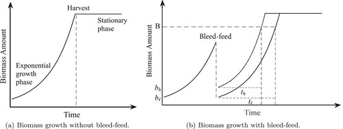
Bioreactor setups can be labour intensive and time-consuming (Yang and Sha 2019). For example, up to 10 hours can be spent during a bioreactor setup (Sharma 2019). This results in long bioreactor occupation times and low throughput levels. Therefore, there is a strong business case in the industry to reduce bioreactor setups and thereby improve throughput. For this purpose, bleed–feed is perceived as a promising technique to skip intermediary bioreactor setups. The main dynamics of bleed–feed are demonstrated in Figure 1(b). When the bleed–feed technique is performed, we extract (‘bleed’) some of the biomass that accumulated inside the bioreactor and add (‘feed’) fresh media for the remaining biomass. The biomass in the remaining culture acts as a seed for the next cultivation and uses the fresh medium to continue growing. Thus bleed–feed technique enables practitioners to skip one setup by prolonging the exponential growth phase. In other words, the bleed–feed technology enables us to produce two cultivations from one setup. The batch is harvested when the second cultivation reaches its predetermined harvest time.¹

Although bleed–feed presents an opportunity to increase throughput, its implementation can be challenging in practice. In particular, we can bleed–feed only in the exponential growth phase for a successful implementation. Otherwise, the technique does not work as the biomass growth stops before the second cultivation. However, the duration of the exponential growth phase is stochastic due to inherent randomness of biological systems. Subsequently, this uncertainty introduces a critical trade-off on the timing of bleed–feed. On the one hand, if we are ‘too late’ to bleed–feed in anticipation of obtaining a higher biomass yield, the bleed–feed opportunity is lost and we harvest the batch with only one cultivation. On the other hand, if we are ‘too early’ to bleed–feed, we may not receive the highest yield from the first cultivation and thus obtain a sub-optimal throughput. Managing this trade-off is crucial for a successful implementation to increase throughput.

The starting biomass amount for the first cultivation (before bleed–feed) is predetermined by manufacturing protocols and cannot be changed. However, the biomanufacturer is allowed to control the starting biomass amount of the second cultivation to achieve the highest benefit from bleed–feed.² For brevity, we call the problem of optimising the starting biomass amount as the replenishment problem. Industry data shows that the replenishment problem itself involves a critical trade-off: when the starting biomass amount is ‘too little’ for the second cultivation, the time needed to achieve a certain biomass amount is likely to be longer. For example, Figure 1(b) illustrates two scenarios with low ($b_{\ell }$) and high ($b_h$) starting biomass amounts in the second cultivation (assuming the same cell growth rate for both cases). Consider a certain biomass amount B. Then, we observe from Figure 1(b) that the time needed to produce B units of biomass is longer (i.e. $t_{\ell }>t_h$) when the starting biomass amount is lower (i.e. $b_{\ell }<b_h$). This behaviour is mainly caused by the exponential growth pattern of biomass and has complex implications on the expected throughput. When we start the second cultivation with a high biomass, this implies that we obtain (extract) only a little biomass from the first cultivation during bleed–feed (thus lowering the throughput). However, the exponential growth phase is likely to be shorter for the second cultivation (thus increasing the throughput). In contrast, when we start the second cultivation with a low biomass, this implies that we obtain (extract) a high biomass yield from the first cultivation. However, the expected throughput of the system may not necessarily be higher, as the time needed to achieve a certain biomass level is longer in the second cultivation. Therefore, starting the second cultivation with ‘too much’ or ‘too little’ biomass would lead to a sub-optimal throughput for the system. By modelling this complex relationship between the initial biomass and the exponential growth duration, we can make better bleed–feed decisions to maximise the expected throughput.

Based on the aforementioned challenges and trade-offs of biomanufacturers, we formulate our research questions as follows:

• What is the optimal bleed–feed time for the first cultivation and the optimal replenishment amount (i.e. starting biomass amount) for the second cultivation in order to maximise the expected throughput?

• What is the added benefit of jointly optimising the bleed–feed time and the replenishment amount in practice?

• How much improvement (in the expected throughput) can we achieve by implementing bleed–feed on current practice? Under which problem settings (e.g. risk of entering the stationary phase, setup duration, etc.) does bleed–feed offer a stronger business case for implementation?

To answer these research questions, we developed a stochastic optimisation model using renewal reward theory and analysed the structural properties of the model. We summarise our contributions as follows. Bleed–feed is a novel technique with a high potential for improving biomanufacturing efficiency. However, its optimal implementation and potential impact is not fully understood. We develop a novel analytical model that combines the biological dynamics with operational trade-offs of bleed–feed. To the best of our knowledge, our study is the first to build an analytical model to jointly optimise the bleed–feed time and the replenishment amount to maximise biomanufacturing throughput. We explore the structural properties of the optimisation problem to generate insights on optimal policies and assess the impact of risks. In addition, we present an industry case study from MSD Animal Health (Boxmeer, the Netherlands) to quantify the potential impact of bleed–feed implementation on practice. To generate broader insights, our numerical experiments assess the performance of three practically relevant strategies as a benchmark: (i) ‘current practice’ which does not implement bleed–feed; (ii) ‘naive bleed–feed policy’ which implements bleed–feed in a risk-averse manner without optimisation and (iii) ‘bleed–feed optimisation’ which assumes a fixed start amount for the second cultivation and optimises the bleed–feed time alone (inspired from Koca et al. 2021). Comparing the performance of these benchmark strategies helps us understand the potential benefits of jointly optimising the bleed–feed time and the replenishment amount on practice. Numerical experiments indicate that our optimisation framework can improve the expected throughput by $17\mathrm{\%}$ compared to current practice.

Our model is generic to address a wide range of applications including biopharmaceutical research and development and large-scale biomanufacturing. Although our research has been primarily inspired by the biomanufacturing industry, applications of bleed–feed technology is relevant to several other industries that use fermentation (e.g. food processing industry for wine or yogurt making, biofuel production with ethanol fermentation, etc.). The outcome of this research has also been shared with a wider audience through industry working group sessions and social media (Nederlandse Biotechnologische Vereniging 2018; MSD 2019). Due to its scalability and potential impact, the research outcomes have been internationally recognised in several platforms including professional societies (IFORS News 2020; IMPACT 2020; European Commission 2020).

The remainder of the paper is organised as follows. We discuss the relevant literature in Section 2. We formulate the renewal model in Section 3 and explore properties of the optimisation problem in Section 4. We present a case study in Section 5 and concluding remarks in Section 6.

2. Literature review

This study is closely related to the following areas: (i) modelling and optimisation of fermentation processes in life sciences, and (ii) applications of Operations Research methodologies in biomanufacturing.

In life sciences, many studies work on improving the fermentation titre (i.e. total biomass obtained from a batch) and productivity (i.e. titre produced in the batch per unit time). Commonly, mass balance equations and kinetic models are built to control fermentation systems (Chang et al. 2011; Villaverde et al. 2016; Nakanishi et al. 2017; D'anjou and Daugulis 2001). Some studies develop predictive models to estimate the relationship between process parameters and fermentation yield. By controlling these parameters, the fermentation titre and productivity are increased (Cunha et al. 2002; Colletti et al. 2011; Handlogten et al. 2018). Additionally, stochastic models are developed to improve fermentation titre and productivity. These studies often focus on controlling process parameters to support cell growth (Kapadi and Gudi 2004; Kachrimanidou et al. 2020; Li et al. 2011; Peroni, Kaisare, and Lee 2005; Wang et al. 2019). However, the life sciences literature mostly focuses on the chemical and biological dynamics of fermentation. To complement the life sciences research, our study combines the biological dynamics of fermentation with operational trade-offs and business implications of bleed–feed, and our insights can be extended to other industries.

The concept of ‘bleed’ (extracting material from the batch) and ‘feed’ (adding fresh medium to the culture) exists in fermentation literature for continuous batch, fed-batch and perfusion fermentation applications (Doran 1995; Walker 2017; Muldowney 2018). However, the implementation of bleed–feed in batch fermentation mode is a new technique and has unique trade-offs and challenges as described in Section 1. Hence, a rigorous analytical modelling of bleed–feed decisions is essential before its implementation, as practitioners need a better understanding on the potential benefits of this new technology.

Applications of Operations Research (OR) methodologies in the biomanufacturing industry is relatively understudied. We refer to Kaminsky and Wang (2015) for a survey of analytical models in biomanufacturing. Limon and Krishnamurthy (2020) analysed a queuing system using matrix-geometric methods to address resource allocation decisions in downstream purification processes. Zeng, Deng, and Yang (2018) proposed a constrained Gaussian process method to predict scaffold biodegradation. Sahling and Hahn (2019) adopted a heuristic approach to address dynamic lot sizing problem in biomanufacturing. In the OR literature, renewal models are mainly studied in the context of maintenance (Sabri-Laghaie and Noorossana 2016; Bei, Zhu, and Coit 2019; Cherkaoui, Huynh, and Grall 2018; Wang 2000; Rebaiaia, Ait-kadi, and Jamshidi 2017) and inventory management (Çetinkaya and Lee 2000; Karamatsoukis and Kyriakidis 2009; Chang and Ho 2010; Boone et al. 2000; Maddah and Jaber 2008). To the best of our knowledge, our study is the first attempt to develop a stochastic optimisation model of bleed–feed decisions (using the renewal reward theory) to optimise biomanufacturing throughput. To date, only a limited number of studies adopted OR methodologies to optimise fermentation processes in biomanufacturing. For example, Xie et al. (2020) adopted Bayesian network approach to model the dependencies between process parameters and quality to improve the performance of fermentation processes. Martagan, Krishnamurthy, and Maravelias (2016) built a Markov Decision Process (MDP) model to determine condition-based harvesting policies to increase fermentation efficiency. However, none of the aforementioned papers addressed the bleed–feed problem.

Koca et al. (2021) presented a first attempt in modelling the bleed–feed problem in biomanufacturing. They built an MDP model to generate condition-based policies that maximise the fermentation yield. Our study is different from Koca et al. (2021) in several fundamental aspects: we optimise both the bleed–feed time and the replenishment amount (i.e. the biomass amount kept inside the batch after bleed–feed) simultaneously. In contrast, Koca et al. (2021) only focus on optimising the bleed–feed time alone and assume a fixed replenishment amount. Our numerical experiments show that joint optimisation of bleed–feed time and replenishment amount can lead to a significant improvement in fermentation throughput. In addition, the replenishment problem itself involves unique trade-offs as explained in Section 1. Besides, we develop an analytical model to maximise throughput; whereas Koca et al. (2021) analyse condition-based policies to maximise yield. This implies that our bleed–feed policy is a time-based policy that takes into account the long setup times in biomanufacturing. Such time-based policies are also practically relevant as they can be easily incorporated into production planning activities.

In summary, our paper contributes to both life sciences and operations research. The bleed–feed problem is new and practically relevant with a high potential to improve biomanufacturing throughput. We address the problem of jointly optimising the bleed–feed time and the replenishment amount by combining the underlying biological dynamics of fermentation with operational trade-offs of bleed–feed. We present an industry case study and provide insights about the potential benefits of bleed–feed.

3. Model formulation

We formulate a renewal model to optimise the bleed–feed time $t_b$ for the first cultivation and starting biomass amount $b_2$ for the second cultivation, with the objective of maximising the expected throughput $R(t_b,b_2)$ (i.e. expected yield per time unit). A fermentation (renewal) cycle starts with a bioreactor setup and continues until a harvest operation. Recall that bleed–feed is performed only in the exponential growth phase but the duration of the exponential growth phase is stochastic (ex-ante). Hence, if the culture is in the exponential growth phase at a certain bleed–feed time $t_b$ (ex-post), then bleed–feed is successful and we obtain two cultivations from one setup. In this case, the second cultivation (after bleed–feed) continues for a fixed processing time $t_h$, which is specified by manufacturing protocols. If the batch is not in the exponential growth phase at time $t_b$ (ex-post), then bleed–feed fails and the batch is harvested with only one cultivation. A new cycle begins each time the batch is harvested.

We build an optimisation model that captures the trade-offs in bleed–feed decisions. On the one hand, the biomanufacturer faces with a trade-off on bleed–feed time $t_b$ (‘too soon’ versus ‘too late’) which affects the chances of successful bleed–feed. On the other hand, there is a trade-off on starting amount $b_2$ (‘too much’ versus ‘too little’) which affects the performance of second cultivation. Both trade-offs have a direct impact on the expected throughput of the system. To establish our objective function and build our optimisation model, we first elaborate on the expected length of a fermentation cycle (Section 3.1) and expected yield obtained in a fermentation cycle (Section 3.2). Table 1 summarises the notation.

Table 1. Notation used in the renewal model.

$b_i$	Initial biomass amount for the ith cultivation
$\mathbb{E}\left[Y\right(t_b,b_2\left)\right]$	Expected yield obtained in a fermentation cycle when bleed–feed is performed at time $t_b$ and the second cultivation starts with $b_2$ units biomass
$f\left(m\right)$	Density of batches that enter the stationary phase at a biomass m
$F\left(m\right)$	Long-run fraction of batches that enter the stationary phase at a biomass of at most m
$g\left(t\right|b)$	Probability density function (pdf) of time to enter the stationary phase given starting amount of b units biomass
$G\left(t\right|b)$	Cumulative distribution function (cdf) of time to enter the stationary phase given starting amount of b units biomass
$m^{\prime }$	The critical biomass amount
$m(t,b)$	Biomass accumulation during the exponential growth phase by time t, when the fermentation starts with b units biomass
μ	Biomass growth rate
$\nu \left(m\right)$	Rate of entering stationary phase under m units of biomass
$R(t_b,b_2)$	Expected throughput when bleed–feed is performed at time $t_b$ and the second cultivation starts with $b_2$ units biomass
s	Bioreactor setup duration
$t_b$	Time to bleed–feed
$T_i$	Random time to enter the stationary phase at the ith cultivation
$t_i$	Realisation of the exponential growth phase's duration for the ith cultivation
$t_h$	Time to harvest a cultivation
$W(t,b)$	Random yield obtained from a cultivation by time t when the starting biomass amount is b

3.1. Length of a fermentation cycle

Each fermentation cycle starts with a bioreactor setup. Setup activities (i.e. cleaning, sterilisation, medium and seed culture transfer) are standardised, and their duration is known in advance. We let s denote the fixed duration of a bioreactor setup.

Our model focuses on a time-based bleed–feed policy, i.e. we define a fixed bleed–feed time $t_b$ ex-ante and do not change our decision during fermentation. In practice, biomanufacturers often prefer to adopt time-based policies, because of production planning restrictions. For example, there is a no-wait constraint such that the batch needs to immediately continue with subsequent purification operations after harvest. In such settings, time-based policies are easier to implement in practice. We note that the bleed–feed time is negligible, as it takes relatively short time (i.e. only 1–2 minutes) with respect to the overall fermentation time (i.e. several days or weeks until the first bleed–feed). Hence, it is practically relevant to assume that the bleed–feed implementation is instantaneous.

Consistent with current good manufacturing practices (CGMPs), the second cultivation (after bleed–feed) needs to be harvested at a fixed harvest time $t_h$. For example, if we decide to implement bleed–feed at time $t_b$, this implies that the bioreactor will be occupied during $t_b+t_h$ time units ($t_b$ for the first and $t_h$ for the second cultivation). Therefore, the fermentation cycle length when we bleed–feed at time $t_b$ is deterministic, and given as $s+t_b+t_h$.

3.2. Expected yield obtained in a fermentation cycle

Let $\mathbb{E}\left[Y\right(t_b,b_2\left)\right]$ denote the expected biomass yield obtained from a fermentation cycle, when we perform bleed–feed at time $t_b$ and start the second cultivation with $b_2$ units biomass. In a fermentation process, the expected biomass yield depends on a complex relationship between the starting biomass amount, random time to enter the stationary phase, and biomass growth rate during the exponential growth phase. Therefore, we establish an analytical model to capture the impact of these critical parameters on the expected yield.

The term $b_i$ denotes the biomass amount at the beginning of cultivation $i\in \{1,2\}$, where i = 1 represents the first cultivation (before bleed–feed) and i = 2 the second one (after bleed–feed). We note that the first cultivation always starts with a certain biomass amount $b_1$, which is prespecified by manufacturing protocols and cannot be changed. However, as part of bleed–feed decisions, the biomanufacturer can control and optimise the starting biomass amount $b_2$ for the second cultivation. The decision $b_2$ affects the risk (probability) of entering the stationary phase.

Let the random variable $T_i$ (with realisation $t_i$) denote the time to enter the stationary phase in cultivation i. The random variable $T_i$ has probability density function $g\left(t_i|b_i\right)$ and distribution function $G\left(t_i|b_i\right)=P(T_i\le t_i|b_i)$ for cultivation i. We note that the density function $g\left(t_i|b_i\right)$ depends on the starting biomass amount $b_i$. We made this modelling assumption based on the analysis of 3 years of industry data. In particular, we observed that the time needed to achieve a certain biomass level is longer when the starting biomass amount is lower (see Figure 1b for an illustration based on real-world data). The underlying intuition of this behaviour can be explained as follows: when we have more biomass, the limited amount of medium depletes faster. As a result, growth inhibition occurs and the fermentation enters the stationary phase earlier. This implies that a high amount of initial biomass $b_2$ does not necessarily lead to high yield, because the process is more likely to enter the stationary phase earlier.

We let the function $m(t,b)$ represents the biomass accumulation by time t (as long as the batch is in the exponential growth phase) when the fermentation starts at time t = 0 with b units of biomass. Based on well-known fermentation models in chemical engineering, the biomass accumulation by time $t\ge 0$ is modelled as (1) $m(t,b)=b{e}^{\mu t},$(1) where μ denotes the growth rate and b the initial biomass (Doran 1995). The exponential growth continues for the cultivation i until the cultivation enters the stationary phase at the realised time $t_i$.

In this setting, the yield obtained from cultivation i is random, because the duration of the exponential phase is random with realisation $t_i$. Therefore, we use Equation (1(1) $m(t,b)=b{e}^{\mu t},$(1) ) to formulate the random yield obtained from cultivation i when we start with $b_i$ units biomass and stop at time t: (2) $W(t,b_i)=\{\begin{array}{ll}{b}_i{e}^{\mu T_i}& \mathrm{i}\mathrm{f}{T}_i\le t,\\ b_i{e}^{\mu t}& \mathrm{i}\mathrm{f}{T}_i>t.\end{array}$(2) Observe from Equation (2(2) $W(t,b_i)=\{\begin{array}{ll}{b}_i{e}^{\mu T_i}& \mathrm{i}\mathrm{f}{T}_i\le t,\\ b_i{e}^{\mu t}& \mathrm{i}\mathrm{f}{T}_i>t.\end{array}$(2) ) that the random yield obtained from cultivation i by time t depends on the realisation of $T_i$. When the exponential growth $T_i$ stops before time t, i.e. $t_i<t$, the biomass yield obtained from cultivation i by time t is $b_i{e}^{\mu t_i}$ (i.e. recall that biomass accumulates only until the realised time $t_i$). Otherwise, the biomass yield is $b_i{e}^{\mu t}$, as the process is still in the exponential growth phase by time t.

We let $\mathbb{E}\left[Y\right(t_b,b_2\left)\right]$ denote the total expected yield obtained from both the first and second cultivations under bleed–feed time $t_b$ (for the first cultivation) and starting biomass amount $b_2$ (for the second cultivation). We formulate $\mathbb{E}\left[Y\right(t_b,b_2\left)\right]$ as (3) $\begin{array}{rl}\mathbb{E}\left[Y\right(t_b,b_2\left)\right]& =\mathbb{E}\left[W\right(t_b,b_1\left)\right]\\ & +(1-G(t_b|b_1\left)\right)\left[\mathbb{E}\right[W(t_h,b_2)]-b_2].\end{array}$(3) In Equation (3(3) $\begin{array}{rl}\mathbb{E}\left[Y\right(t_b,b_2\left)\right]& =\mathbb{E}\left[W\right(t_b,b_1\left)\right]\\ & +(1-G(t_b|b_1\left)\right)\left[\mathbb{E}\right[W(t_h,b_2)]-b_2].\end{array}$(3) ), $\mathbb{E}\left[W\right(t_b,b_1\left)\right]$ represents the expected yield of the first cultivation. Using Equation (2(2) $W(t,b_i)=\{\begin{array}{ll}{b}_i{e}^{\mu T_i}& \mathrm{i}\mathrm{f}{T}_i\le t,\\ b_i{e}^{\mu t}& \mathrm{i}\mathrm{f}{T}_i>t.\end{array}$(2) ), $\mathbb{E}\left[W\right(t_b,b_1\left)\right]$ can be written as $\mathbb{E}\left[W\right(t_b,b_1\left)\right]={\int }_0^{t_b}{b}_1{e}^{\mu t_1}g\left(t_1|b_1\right)\mathrm{d}{t}_1+{\int }_{t_b}^{\mathrm{\infty }}{b}_1{e}^{\mu t_b}g\left(t_1|b_1\right)\mathrm{d}{t}_1$. The first summand represents the biomass produced from the first cultivation when bleed–feed fails ($t_1\le t_b$). The second summand is the biomass production in the first cultivation when bleed–feed is successful ($t_1>t_b$). In this case, the bleed–feed time limits the cell growth, and yield becomes $b_1{e}^{\mu t_b}$. Thus we can also rewrite the second summand as ${\int }_{t_b}^{\mathrm{\infty }}{b}_1{e}^{\mu t_b}g\left(t_1|b_1\right)\mathrm{d}{t}_1=(1-G(t_b|b_1\left)\right)b_1{e}^{\mu t_b}$. The term $1-G\left(t_b|b_1\right)$ in (3(3) $\begin{array}{rl}\mathbb{E}\left[Y\right(t_b,b_2\left)\right]& =\mathbb{E}\left[W\right(t_b,b_1\left)\right]\\ & +(1-G(t_b|b_1\left)\right)\left[\mathbb{E}\right[W(t_h,b_2)]-b_2].\end{array}$(3) ) represents the probability of a successful bleed–feed. If bleed–feed is successful, then we produce the second cultivation with the expected yield $\mathbb{E}\left[W\right(t_h,b_2\left)\right]-b_2={\int }_0^{t_h}{b}_2{e}^{\mu t_2}g\left(t_2|b_2\right)\mathrm{d}{t}_2+{\int }_{t_h}^{\mathrm{\infty }}{b}_2{e}^{\mu t_h}g\left(t_2|b_2\right)\mathrm{d}{t}_2-b_2$. The first summand represents the yield obtained from the second cultivation when the exponential growth ends before the harvest time, $t_2\le t_h$. The second summand captures the case when the exponential growth does not end before the prespecified harvest time, $t_2>t_h$. When $t_2>t_h$, the harvest time $t_h$ limits the biomass growth, and hence the cultivation yield becomes $b_2{e}^{\mu t_h}$. Therefore, we have ${\int }_{t_h}^{\mathrm{\infty }}{b}_2{e}^{\mu t_h}g\left(t_2|b_2\right)\mathrm{d}{t}_2=(1-G(t_h|b_2\left)\right)b_2{e}^{\mu t_h}$. If bleed–feed is successful, we subtract $b_2$ from the second cultivation yield since $b_2$ was produced in the first cultivation and was already in the batch during the second. The randomness in the yield is captured by probability distribution of the exponential growth phase's duration (i.e. $g\left(t_i\right|b_i)$ for $i=\{1,2\}$).

Recall that the replenishment problem involves a critical relationship between the starting amount $b_2$ and the duration of the exponential growth phase. Because of the exponential growth pattern described in Equation (1(1) $m(t,b)=b{e}^{\mu t},$(1) ), it takes longer to achieve a certain biomass amount when $b_2$ is too small (see Figure 1b for an illustration). To capture this relationship analytically, we define a rate function: let $\nu \left(m\right)$ denote the rate of entering the stationary phase when there are m units biomass inside the bioreactor. The rate function $\nu \left(m\right)$ can be obtained from industry data (see Appendix for details). In our analytical model, we use the rate function $\nu \left(m\right(t,b_i\left)\right)$ to estimate the probability density function $g\left(t_i|b_i\right)$, as explained in Section 3.2.1.

3.2.1. Establishing the probability distribution to stationary phase from the rate function

We now establish the probability density function $g\left(t|b\right)$ from the rate function $\nu \left(m\right)$. Consider a random time to enter stationary phase T, with distribution function $G\left(t|b\right)=P(T\le t|b),t\ge 0,$where b represents the initial biomass. The function $\nu \left(m\right)$ is the transition rate to the stationary phase when the biomass amount is m. Then, we have $\begin{array}{rl}g\left(t|b\right)\mathrm{d}t& =P(T>t|b)\cdot P(T<t+\mathrm{d}t|T>t,b)\\ & =(1-G(t|b\left)\right)\nu \left(m\right(t,b\left)\right)\mathrm{d}t.\end{array}$Hence, $\frac{g\left(t|b\right)}{1-G\left(t|b\right)}=\nu \left(m\right(t,b\left)\right)$and integrating this equation yields (by using that $G(0,b)=0$) $\log (1-G(t|b\left)\right)=-{\int }_0^t\nu \left(m\right(s,b\left)\right)\mathrm{d}s,$thus, $1-G\left(t|b\right)=e^{-{\int }_0^t\nu \left(m\right(s,b\left)\right)\mathrm{d}s},t\ge 0.$The probability density function is $g\left(t|b\right)=G^{\prime }\left(t|b\right)$. For the expectation, we get $\mathbb{E}\left[T\right|b]={\int }_0^{\mathrm{\infty }}(1-G\left(t|b\right))\mathrm{d}t={\int }_0^{\mathrm{\infty }}{e}^{-{\int }_0^t\nu \left(m\right(s,b\left)\right)\mathrm{d}s}\mathrm{d}t.$Thus once we obtain the rate function $\nu \left(m\right)$ from the industry data (as explained in Appendix) we can establish the probability density function of entering the stationary phase $g\left(t|b\right)$.

3.3. The objective function and the optimisation model

We formulate our optimisation model to determine a bleed–feed policy $\pi (t_b,b_2)$ that maximises the expected throughput $R(t_b,b_2)$. By using the fermentation cycle length presented in Section 3.1, and the expected yield of a fermentation cycle in Section 3.2, we formulate our objective function as follows: (4) $\begin{array}{rl}& R(t_b,b_2)\\ & =\frac{\mathbb{E}\left[W\right(t_b,b_1\left)\right]+(1-G(t_b|b_1\left)\right)\left[\mathbb{E}\right[W(t_h,b_2)]-b_2]}{s+t_b+t_h}.\end{array}$(4) Equation (4(4) $\begin{array}{rl}& R(t_b,b_2)\\ & =\frac{\mathbb{E}\left[W\right(t_b,b_1\left)\right]+(1-G(t_b|b_1\left)\right)\left[\mathbb{E}\right[W(t_h,b_2)]-b_2]}{s+t_b+t_h}.\end{array}$(4) ) denotes the expected throughput (i.e.expected yield produced per unit time) as a function of the bleed–feed time $t_b$ (for the first cultivation) and starting amount $b_2$ (for the second cultivation). Using Equation (4(4) $\begin{array}{rl}& R(t_b,b_2)\\ & =\frac{\mathbb{E}\left[W\right(t_b,b_1\left)\right]+(1-G(t_b|b_1\left)\right)\left[\mathbb{E}\right[W(t_h,b_2)]-b_2]}{s+t_b+t_h}.\end{array}$(4) ), we solve the following two-dimensional optimisation problem to maximise the expected throughput: (5) $\begin{array}{rl}max& R(t_b,b_2)\\ \mathrm{s}.\mathrm{t}.& 0<b_2\le b_1,\\ & 0\le t_b\le t_h.\end{array}$(5) In problem (5(5) $\begin{array}{rl}max& R(t_b,b_2)\\ \mathrm{s}.\mathrm{t}.& 0<b_2\le b_1,\\ & 0\le t_b\le t_h.\end{array}$(5) ), the first constraint ensures that the starting biomass $b_2$ of the second cultivation is lower than $b_1$. The amount $b_1$ represents the maximum possible amount to start a cultivation, as defined by current manufacturing protocols. Nevertheless, the protocols provide an opportunity to control the biomass amount $b_2$ on the range $(0,b_1]$, as part of bleed–feed decisions. In common practice, the harvest time $t_h$ represents a prespecified bound on the cultivation processing time. Hence, the second constraint ensures that the bleed–feed time $t_b$ does not exceed the predefined fermentation time $t_h$. Our model takes these practical boundaries into account to find an optimal $\pi (t_b,b_2)$ to maximise throughput $R(t_b,b_2)$.

For computational efficiency, we can reduce the problem (5(5) $\begin{array}{rl}max& R(t_b,b_2)\\ \mathrm{s}.\mathrm{t}.& 0<b_2\le b_1,\\ & 0\le t_b\le t_h.\end{array}$(5) ) into two sequential, one-dimensional optimisation problems as follows. Consider our objective function: $\begin{array}{rl}& \underset{t_b,b_2}{max}R(t_b,b_2)\\ & =\underset{t_b}{max}\frac{1}{s+t_b+t_h}\\ & \times \left[\mathbb{E}\right[W(t_b,b_1)+(1-G(t_b|b_1\left)\right)\underset{b_2}{max}\left(\mathbb{E}\right[W(t_h,b_2)]\\ & -b_2\left)\right].\end{array}$Note that the expected yield obtained from the second cultivation $\mathbb{E}\left[W\right(t_h,b_2\left)\right]$ depends only on the starting amount of the second cultivation $b_2$ and not on the bleed–feed time $t_b$. Hence, we can first solve the inner optimisation problem (the first one-dimensional problem) to find $b_2^{\ast }$ maximising $\mathbb{E}\left[W\right(t_h,b_2\left)\right]-b_2$. Then, we can substitute $b_2^{\ast }$ in the original optimisation problem to have the second one-dimensional problem as $\begin{array}{rl}& =\underset{t_b}{max}\frac{1}{s+t_b+t_h}\left[\mathbb{E}\right[W(t_b,b_1)+(1-G(t_b|b_1\left)\right)\\ & \times \left(\mathbb{E}\right[W(t_h,b_2^{\ast })]-b_2^{\ast })].\end{array}$

4. Properties of the optimisation problem

In this section, we consider the optimisation problem (5(5) $\begin{array}{rl}max& R(t_b,b_2)\\ \mathrm{s}.\mathrm{t}.& 0<b_2\le b_1,\\ & 0\le t_b\le t_h.\end{array}$(5) ) and explore the properties of the expected throughput function $R(t_b,b_2)$. We generate insights on optimal policies (Section 4.1) and analyse the impact of system's risks (Section 4.2).

4.1. Insights on optimal policies

Insights on the optimal bleed–feed time ${\mathit{t}}_{\mathit{b}}^{\mathbf{\ast }}$. The cell culture does not transition to the stationary phase before a certain biomass amount is reached. We refer to this biomass amount as the ‘critical biomass level ’ $m^{\prime }$. Hence, the probability of entering to the stationary phase is typically zero when the actual biomass amount is below this critical biomass $m^{\prime }$. In practice, the value of critical biomass $m^{\prime }$ is known and depends on the cell culture and equipment used in fermentation. Subsequently, the ‘critical biomass time’ $t^{\prime }$ denotes the time when $m^{\prime }$ is reached. Then, we have $m^{\prime }=b_i{e}^{\mu t^{\prime }}$, and hence $t^{″}=\frac{1}{\mu }\log \frac{m^{\prime }}{b_i}$. Therefore, $\nu \left(m\right)=0$ for $m\le m^{\prime }$, and $g\left(t\right|b_i)=0$ for $t\le t^{\prime }$.

We now explore the impact of parameters $m^{\prime }$ and $t^{\prime }$ on optimal bleed–feed policies. For this purpose, we let $\pi (t_b,b_2)$ represent a bleed–feed policy which performs the bleed–feed at time $t_b$ and starts the second cultivation with $b_2$ units of biomass. We formalise our insights in Lemma 4.1 and Proposition 4.1.

Lemma 4.1

For a fixed biomass amount $b_2$, the expected biomass yield $\mathbb{E}\left[Y\right(t_b,b_2\left)\right]$ under the bleed–feed policy $\pi (t_b,b_2)$ increases in the bleed-feed time $t_b$ for $0\le t_b\le t^{\prime }$, where $t^{\prime }$ is the critical biomass time.

Proof.

Take two policies: $\pi (t_b,b_2)$ and $\pi (t^{\prime },b_2)$, where $0\le t_b\le t^{\prime }$, for all $b_2$. We compare the expected yield under these policies and show $\mathbb{E}\left[Y\right(t_b,b_2\left)\right]\le \mathbb{E}\left[Y\right(t^{\prime },b_2\left)\right]$ for $0\le t_b\le t^{\prime }$. From the fact that $g\left(t_b\right|b_i)=0$ for $t_b\le t^{\prime }$, we have $\begin{array}{rl}\mathbb{E}\left[Y\right(t_b,b_2\left)\right]& =b_1{e}^{\mu t_b}+\mathbb{E}\left[W\right(t_h,b_2\left)\right]-b_2\le b_1{e}^{\mu t^{\prime }}\\ & +\mathbb{E}\left[W\right(t_h,b_2\left)\right]-b_2=\mathbb{E}\left[Y\right(t^{\prime },b_2\left)\right],\end{array}$which concludes the proof.

Lemma 4.1 indicates that the expected yield $\mathbb{E}\left[Y\right(t_b,b_2\left)\right]$ obtained from the bleed–feed policy $\pi (t_b,b_2)$ is increasing in bleed–feed time $t_b$ when $0\le t_b\le t^{\prime }$. However, this insight is not necessarily valid for the expected throughput. This is because the fermentation cycle time also increases when the expected yield obtained from the batch increases in $t_b$ (where $0\le t_b\le t^{\prime }$). When the additional yield does not outweigh the extended fermentation time, the expected throughput may decrease in $t_b$ (when $0\le t_b\le t^{\prime }$). From a practical perspective, Lemma 4.1 implies that it is optimal not to perform bleed–feed before the critical biomass time $t^{\prime }$. We further explore this insight in Proposition 4.1.

Proposition 4.1

$R(t_b,b_2)$ is convex in $t_b$ for $0\le t_b\le t^{\prime }$ and fixed $b_2$, if the following condition holds: (6) $\frac{\mu }{2}>\frac{1}{s+t_h}.$(6)

Proof.

Consider a bleed–feed policy $\pi (t_b,b_2)$, where $0\le t_b\le t^{\prime }$ for a fixed $b_2$. Under the policy $\pi (t_b,b_2)$, we prove convexity of the throughput function by showing that $\frac{{\mathrm{\partial }}^{2}R(t_b,b_2)}{\mathrm{\partial }{t}_b^2}>0$. Since $g\left(t_b\right|b_i)=0$ for $t_b\le t^{\prime }$, we write $R(t_b,b_2)$ as (7) $R(t_b,b_2)=\frac{b_1{e}^{\mu t_b}+\mathbb{E}\left[W\right(t_h,b_2\left)\right]-b_2}{s+t_b+t_h}.$(7) Hence, (8) $\begin{array}{rl}\frac{{\mathrm{\partial }}^{2}R(t_b,b_2)}{\mathrm{\partial }{t}_b^2}& =\frac{{\mu }^2{b}_1{e}^{\mu t_b}}{s+t_b+t_h}-\frac{2\mu b_1{e}^{\mu t_b}}{(s+t_b+t_h{)}^2}\\ & +\frac{2b_1{e}^{\mu t_b}}{(s+t_b+t_h{)}^3}+\frac{2\mathbb{E}\left[W\right(t_h,b_2\left)\right]-2b_2}{(s+t_b+t_h{)}^3}.\end{array}$(8) We now show that if (6(6) $\frac{\mu }{2}>\frac{1}{s+t_h}.$(6) ) holds, then $\frac{{\mathrm{\partial }}^{2}R(t_b,b_2)}{\mathrm{\partial }{t}_b^2}>0$. Rearranging (6(6) $\frac{\mu }{2}>\frac{1}{s+t_h}.$(6) ) we have that $0>\frac{1}{s+t_h}-\frac{\mu }{2}.$Multiplying both sides of the inequality by μ and rearranging the terms we obtain (9) $\begin{array}{rl}0& >\frac{\mu }{s+t_b+t_h}-\frac{{\mu }^2}{2}\end{array}$(9) (10) $\begin{array}{rl}& >\frac{\mu }{s+t_b+t_h}-\frac{1}{(s+t_b+t_h{)}^2}-\frac{{\mu }^2}{2},\end{array}$(10) where (9(9) $\begin{array}{rl}0& >\frac{\mu }{s+t_b+t_h}-\frac{{\mu }^2}{2}\end{array}$(9) ) follows since $\frac{\mu }{2}>\frac{1}{s+t_h}\ge \frac{1}{s+t_b+t_h}$ for $t_b\ge 0$, and (10(10) $\begin{array}{rl}& >\frac{\mu }{s+t_b+t_h}-\frac{1}{(s+t_b+t_h{)}^2}-\frac{{\mu }^2}{2},\end{array}$(10) ) follows from the fact that $\frac{1}{(s+t_b+t_h{)}^2}>0$. Multiplying both sides of (10(10) $\begin{array}{rl}& >\frac{\mu }{s+t_b+t_h}-\frac{1}{(s+t_b+t_h{)}^2}-\frac{{\mu }^2}{2},\end{array}$(10) ) by $\frac{2b_1{e}^{\mu t_b}}{s+t_b+t_h}$ we obtain (11) $\begin{array}{rl}0& >\frac{2\mu b_1{e}^{\mu t_b}}{(s+t_b+t_h{)}^2}-\frac{2b_1{e}^{\mu t_b}}{(s+t_b+t_h{)}^3}-\frac{{\mu }^2{b}_1{e}^{\mu t_b}}{s+t_b+t_h}\\ & >\frac{2\mu b_1{e}^{\mu t_b}}{(s+t_b+t_h{)}^2}-\frac{2b_1{e}^{\mu t_b}}{(s+t_b+t_h{)}^3}-\frac{{\mu }^2{b}_1{e}^{\mu t_b}}{s+t_b+t_h}\\ & -\frac{2\mathbb{E}\left[W\right(t_h,b_2\left)\right]-2b_2}{(s+t_b+t_h{)}^3},\end{array}$(11) where (11(11) $\begin{array}{rl}0& >\frac{2\mu b_1{e}^{\mu t_b}}{(s+t_b+t_h{)}^2}-\frac{2b_1{e}^{\mu t_b}}{(s+t_b+t_h{)}^3}-\frac{{\mu }^2{b}_1{e}^{\mu t_b}}{s+t_b+t_h}\\ & >\frac{2\mu b_1{e}^{\mu t_b}}{(s+t_b+t_h{)}^2}-\frac{2b_1{e}^{\mu t_b}}{(s+t_b+t_h{)}^3}-\frac{{\mu }^2{b}_1{e}^{\mu t_b}}{s+t_b+t_h}\\ & -\frac{2\mathbb{E}\left[W\right(t_h,b_2\left)\right]-2b_2}{(s+t_b+t_h{)}^3},\end{array}$(11) ) follows from $\frac{2\mathbb{E}\left[W\right(t_h,b_2\left)\right]-2b_2}{(s+t_b+t_h{)}^3}>0$. Rearranging (11(11) $\begin{array}{rl}0& >\frac{2\mu b_1{e}^{\mu t_b}}{(s+t_b+t_h{)}^2}-\frac{2b_1{e}^{\mu t_b}}{(s+t_b+t_h{)}^3}-\frac{{\mu }^2{b}_1{e}^{\mu t_b}}{s+t_b+t_h}\\ & >\frac{2\mu b_1{e}^{\mu t_b}}{(s+t_b+t_h{)}^2}-\frac{2b_1{e}^{\mu t_b}}{(s+t_b+t_h{)}^3}-\frac{{\mu }^2{b}_1{e}^{\mu t_b}}{s+t_b+t_h}\\ & -\frac{2\mathbb{E}\left[W\right(t_h,b_2\left)\right]-2b_2}{(s+t_b+t_h{)}^3},\end{array}$(11) ) we obtain (12) $\begin{array}{rl}\frac{{\mathrm{\partial }}^{2}R(t_b,b_2)}{\mathrm{\partial }{t}_b^2}& =\frac{{\mu }^2{b}_1{e}^{\mu t_b}}{s+t_b+t_h}-\frac{2\mu b_1{e}^{\mu t_b}}{(s+t_b+t_h{)}^2}\\ & +\frac{2b_1{e}^{\mu t_b}}{(s+t_b+t_h{)}^3}\\ & +\frac{2\mathbb{E}\left[W\right(t_h,b_2\left)\right]-2b_2}{(s+t_b+t_h{)}^3}>0,\end{array}$(12) which completes the proof.

Proposition 4.1 presents a sufficient condition under which the expected throughput function $R(t_b,b_2)$ is convex in $t_b$ when $0\le t_b\le t^{\prime }$ for a given $b_2$. Condition (6(6) $\frac{\mu }{2}>\frac{1}{s+t_h}.$(6) ) sets a lower bound on the growth rate μ in terms of fermentation processing rate (i.e.setup time s and harvest time $t_h$). This condition may not hold when the biomass growth rate μ is too small or when the fermentation setup and cultivation harvest time is too short. Nevertheless, we validated with industry data that Condition (6(6) $\frac{\mu }{2}>\frac{1}{s+t_h}.$(6) ) is mild and holds for a wide range of practically-relevant settings (i.e.Condition (6(6) $\frac{\mu }{2}>\frac{1}{s+t_h}.$(6) ) holds for the base case and all other scenarios considered in case study in Section 5).

Convexity of the expected throughput $R(t_b,b_2)$ in $0\le t_b\le t^{\prime }$ implies that we need to analyse the boundary conditions (i.e. when $t_b=0$ and $t_b=t^{\prime }$) to maximise throughput. Therefore, we compare the two extreme scenarios, namely the bleed–feed policies $\pi (t^{\prime },b_2)$ (when we bleed–feed at time $t^{\prime }$) and $\pi (0,b_2)$ (when we bleed–feed at t = 0) for a fixed $b_2$. Note that bleed–feeding at $t_b=0$ represents the case when bleed–feed is not implemented. Next, we observe that bleed-feeding at time $t^{\prime }$ is better than bleed–feeding at time 0, if: (13) $\begin{array}{rl}R(t^{\prime },b_2)& =\frac{\mathbb{E}\left[W\right(t^{\prime },b_1\left)\right]+\mathbb{E}\left[W\right(t_h,b_2\left)\right]-b_2}{s+t^{\prime }+t_h}\\ & \ge \frac{\mathbb{E}\left[W\right(0,b_1\left)\right]+\mathbb{E}\left[W\right(t_h,b_2\left)\right]-b_2}{s+t_h}\\ & =R(0,b_2).\end{array}$(13) In (13(13) $\begin{array}{rl}R(t^{\prime },b_2)& =\frac{\mathbb{E}\left[W\right(t^{\prime },b_1\left)\right]+\mathbb{E}\left[W\right(t_h,b_2\left)\right]-b_2}{s+t^{\prime }+t_h}\\ & \ge \frac{\mathbb{E}\left[W\right(0,b_1\left)\right]+\mathbb{E}\left[W\right(t_h,b_2\left)\right]-b_2}{s+t_h}\\ & =R(0,b_2).\end{array}$(13) ), $\mathbb{E}\left[W\right(t^{\prime },b_1\left)\right]=b_1{e}^{\mu t^{\prime }}=m^{\prime }$ and $\mathbb{E}\left[W\right(0,b_1\left)\right]=b_1$. Rearranging the terms, we obtain (14) $\begin{array}{rl}& \frac{m^{\prime }}{s+t^{\prime }+t_h}-\frac{b_1}{s+t_h}\ge \frac{\mathbb{E}\left[W\right(t_h,b_2\left)\right]-b_2}{s+t_h}\\ & -\frac{\mathbb{E}\left[W\right(t_h,b_2\left)\right]-b_2}{s+t^{\prime }+t_h}.\end{array}$(14) When we bleed–feed earlier than $t^{\prime }$, the bleed–feed is successful because there is no risk of entering the stationary phase when $t_b\le t^{\prime }$. Therefore, the expected yield produced from the second cultivation $\mathbb{E}\left[W\right(t_h,b_2\left)\right]$ is constant for all $t_b\le t^{\prime }$ for a fixed $b_2$. On one hand, if we bleed–feed at $t^{\prime }$ instead of at time 0, the fermentation cycle increases, and hence the throughput from the second cultivation decreases. On the other hand, bleed–feeding at time $t^{\prime }$ leads to increased yield from the first cultivation compared to the case when we bleed–feed at time 0. Thus  (14(14) $\begin{array}{rl}& \frac{m^{\prime }}{s+t^{\prime }+t_h}-\frac{b_1}{s+t_h}\ge \frac{\mathbb{E}\left[W\right(t_h,b_2\left)\right]-b_2}{s+t_h}\\ & -\frac{\mathbb{E}\left[W\right(t_h,b_2\left)\right]-b_2}{s+t^{\prime }+t_h}.\end{array}$(14) ) implies that, if the decrease in throughput in the second cultivation is smaller than the increase in the throughput from the first cultivation, than bleed–feeding at time $t^{\prime }$ is better than bleed–feeding at time 0, and vice versa. In addition, we validated that (14(14) $\begin{array}{rl}& \frac{m^{\prime }}{s+t^{\prime }+t_h}-\frac{b_1}{s+t_h}\ge \frac{\mathbb{E}\left[W\right(t_h,b_2\left)\right]-b_2}{s+t_h}\\ & -\frac{\mathbb{E}\left[W\right(t_h,b_2\left)\right]-b_2}{s+t^{\prime }+t_h}.\end{array}$(14) ) holds for the industry case study presented in Section 5.

Our analysis presents a sufficient condition under which the optimal bleed–feed time is at $t^{\prime }$ or later, where $t^{\prime }=\frac{1}{\mu }\log \frac{m^{\prime }}{b_1}$ and $m^{\prime }$ is fixed. Hence, when the initial biomass level $b_1$ or growth rate μ is small, the time to reach the critical biomass amount $t^{\prime }$ is high. In such cases, the left-hand side of (14(14) $\begin{array}{rl}& \frac{m^{\prime }}{s+t^{\prime }+t_h}-\frac{b_1}{s+t_h}\ge \frac{\mathbb{E}\left[W\right(t_h,b_2\left)\right]-b_2}{s+t_h}\\ & -\frac{\mathbb{E}\left[W\right(t_h,b_2\left)\right]-b_2}{s+t^{\prime }+t_h}.\end{array}$(14) ) decreases, while the right-hand side increases. As a result, bleed–feeding at time 0 might be better than bleed–feeding at time $t^{\prime }$. We further investigate the optimal bleed–feed time through a comprehensive numerical analysis in Section 5.

Insights on the optimal starting biomass amount for the second cultivation ${\mathit{b}}_{\mathbf{2}}^{\mathbf{\ast }}$. Recall that the yield $\mathbb{E}\left[W\right(t_h,b_2\left)\right]-b_2$ obtained from the second cultivation (when the bleed–feed is successful) depends only on $b_2$. Hence, the amount $b_2$ for which $\mathbb{E}\left[W\right(t_h,b_2\left)\right]-b_2$ is maximised would be the optimal start amount for the second cultivation. Proposition 4.2 shows that $\mathbb{E}\left[W\right(t_h,b_2\left)\right]-b_2$ is concave in $b_2$ for a special case, where the rate function $\nu \left(m\right)$ is linearly increasing in the biomass m.

Proposition 4.2

$\mathbb{E}\left[W\right(t_h,b_2\left)\right]-b_2$ is concave in $b_2$ when the rate function $\nu \left(m\right)$ is linearly increasing in the biomass amount m.

Proof.

Take a linearly increasing rate function $\nu \left(m\right)=cm$ for c>0 (i.e.$\nu \left(m\right(t,b_2\left)\right)=cm(t,b_2)=c{b}_2{e}^{\mu t}$). We prove concavity of $\mathbb{E}\left[W\right(t_h,b_2\left)\right]-b_2$ in $b_2$ by showing that $\frac{{\mathrm{\partial }}^2\left(\mathbb{E}\right[W(t_h,b_2)]-b_2)}{\mathrm{\partial }{b}_2^2}<0$. Using $\nu \left(m\right(t,b_2\left)\right)=cm(t,b_2)=c{b}_2{e}^{\mu t}$, we have $\begin{array}{rl}& \mathbb{E}\left[W\right(t_h,b_2\left)\right]-b_2\\ & ={\int }_0^{t_h}{b}_2{e}^{\mu t_2}g\left(t_2|b_2\right)\mathrm{d}{t}_2+(1-G(t_h|b_2\left)\right)b_2{e}^{\mu t_h}-b_2\\ & =-b_2+b_2{e}^{-\frac{c{b}_2(-1+e^{\mu t_h})}{\mu }+\mu t_h}\\ & +\frac{b_2(c-c{e}^{\frac{c{b}_2-c{b}_2{e}^{\mu t_h+{\mu }^2{t}_h}}{\mu }})+\mu -e^{-\frac{c{b}_2(-1+\mu t_h)}{\mu }}\mu }{c}.\end{array}$Then, $\begin{array}{rl}& \frac{{\mathrm{\partial }}^2\left(\mathbb{E}\right[W(t_h,b_2)]-b_2)}{\mathrm{\partial }{b}_2^2}\\ & =-\frac{c{e}^{-\frac{c{b}_2(-1+e^{\mu t_h})}{\mu }}(-1+e^{\mu t_h}{)}^2}{\mu }<0,\end{array}$which completes the proof.

Proposition 4.2 focuses on a special case of the problem to study the concavity of $\mathbb{E}\left[W\right(t_h,b_2\left)\right]-b_2$ in $b_2$. We note that the complex nature of the rate function $\nu \left(m\right)$ challenges the proof of Proposition 4.2 for more generic cases.

We now present a boundary for the optimal start amount $b_2^{\ast }$ by using the relations obtained from industry data: $\nu \left(m\right)=0$ for $m\le m^{\prime }$ and $\nu \left(m\right)=1$ for m>H, where H denotes the maximum possible biomass obtained from a cultivation due to limitations in cell viability and growth. When $\nu \left(m\right)=0$, the first derivative of $\mathbb{E}\left[W\right(t_h,b_2\left)\right]-b_2$ is equal to $e^{\mu t_h}-1$, which is positive. This means that the expected yield obtained from the second cultivation is increasing in $b_2$. Thus we reach the critical biomass amount until the second cultivation ends, i.e. $b_2{e}^{\mu t_h}=m^{\prime }$, resulting in at least $b_2=\frac{m^{\prime }}{e^{\mu t_h}}$. Similarly, when $\nu \left(m\right)=1$, the first derivative of $\mathbb{E}\left[W\right(t_h,b_2\left)\right]-b_2$ is equal to $-1$, meaning that the expected yield obtained from the second cultivation is decreasing in $b_2$. Then, we do not to exceed the maximum biomass amount that can be produced until the second cultivation ends, i.e. $b_2{e}^{\mu t_h}=H$, resulting in at most $b_2=\frac{H}{e^{\mu t_h}}$. Since we have a constraint on $b_2$ as $b_2\le b_1$ in problem (5(5) $\begin{array}{rl}max& R(t_b,b_2)\\ \mathrm{s}.\mathrm{t}.& 0<b_2\le b_1,\\ & 0\le t_b\le t_h.\end{array}$(5) ), the upper bound would be $min(b_1,\frac{H}{e^{\mu t_h}})$. As a result $b_2^{\ast }$ would be in the interval $[\frac{m^{\prime }}{e^{\mu t_h}},min(b_1,\frac{H}{e^{\mu t_h}}\left)\right]$.

4.2. Insights on the risk of entering the stationary phase

We evaluate the impact of risk of entering the stationary phase on the expected throughput. For this purpose, we consider two batches with identical initial biomass amount $b_1$ and growth rate μ, on which we implement the same bleed–feed policy $\pi (t_b,b_2)$. We shall assume that these two batches are identical except for their risk of entering the stationary phase. To assess their difference in risk, we adopt the concept of stochastic ordering (Ross 1996).

Proposition 4.3

If the time to enter the stationary phase for batch A is stochastically larger than the time to enter the stationary phase for batch B, the throughput of batch A under a bleed–feed policy $\pi (t_b,b_2)$ is higher than the throughput of batch B under the same bleed–feed policy.

Proof.

Take two batches as batch A and B with identical $b_1$ and μ, with the rate function of entering the stationary phase for batch B dominating A. Let $G^j$ denote the distribution function of time to enter stationary phase for batch $j=\{A,B\}$ and $T_i^j$ denote the random time to enter stationary phase for batch $j=\{A,B\}$; $T_i^A$ being distributed according to $G^A$, and $T_i^B$ according to $G^B$, for cultivation $i=\{1,2\}$. Then, $t_i^j$ denotes the realisation of random time to enter stationary phase for batch $j=\{A,B\}$ in cultivation $i=\{1,2\}$. Take a bleed–feed policy $\pi (t_b,b_2)$. $R^j(t_b,b_2)$ denotes the throughput and $\mathbb{E}\left[Y^j\right(t_b,b_2\left)\right]$ the expected yield under bleed–feed policy $\pi (t_b,b_2)$ for batch $j=\{A,B\}$. From Equation (3(3) $\begin{array}{rl}\mathbb{E}\left[Y\right(t_b,b_2\left)\right]& =\mathbb{E}\left[W\right(t_b,b_1\left)\right]\\ & +(1-G(t_b|b_1\left)\right)\left[\mathbb{E}\right[W(t_h,b_2)]-b_2].\end{array}$(3) ), the expected yield for batch j under policy $\pi (t_b,b_2)$ is given as: $\begin{array}{rl}\mathbb{E}\left[Y^j\right(t_b,b_2\left)\right]& =\mathbb{E}\left[W^j\right(t_b,b_1\left)\right]+(1-G^j(t_b|b_1\left)\right)\\ & \times \left[\mathbb{E}\right[W^j(t_h,b_2)]-b_2].\end{array}$Because the rate function of entering the stationary phase for batch B dominates that of A, the random time to enter stationary phase for batch A is stochastically larger than that of batch B, $T_i^A⪰T_i^B$. By coupling (Proposition 9.2.2 from Ross 1996), we have $t_i^A>t_i^B$ for every realisation of $T_i^A$ and $T_i^B$ (considering a given cultivation i). Thus for the yield in the batch from the second cultivation we can say that $W^A(t_h,b_2)\ge W^B(t_h,b_2)$ for each realisation, so $\mathbb{E}\left[W^A\right(t_h,b_2\left)\right]\ge \mathbb{E}\left[W^B\right(t_h,b_2\left)\right]$ by Proposition 9.1.2 from Ross (1996). Similarly, we can say that $\mathbb{E}\left[W^A\right(t_b,b_1\left)\right]\ge \mathbb{E}\left[W^B\right(t_b,b_1\left)\right]$. By definition of stochastic ordering, $1-G^A\left(t_b|b_1\right)>1-G^B\left(t_b|b_1\right)$ holds. Thus $\mathbb{E}\left[Y^A\right(t_b,b_2\left)\right]\ge \mathbb{E}\left[Y^B\right(t_b,b_2\left)\right]$. If we divide both sides by the cycle length under the bleed–feed policy $\pi (t_b,b_2)$ we obtain $\begin{array}{rl}{R}^A(t_b,b_2)& =\frac{\mathbb{E}\left[Y^A\right(t_b,b_2\left)\right]}{s+t_b+t_h}\ge \frac{\mathbb{E}\left[Y^B\right(t_b,b_2\left)\right]}{s+t_b+t_h}\\ & =R^B(t_b,b_2),\end{array}$which completes the proof.

If the rate function to enter stationary phase for one batch stochastically dominates the other one (when everything else is identical), then the latter batch has stochastically larger time to enter stationary phase than the former. This means that, when a batch has higher rate to enter stationary phase, it is more likely for this batch to stop growing at early biomass levels. Hence, the expected yield and the expected throughput for this batch will be lower.

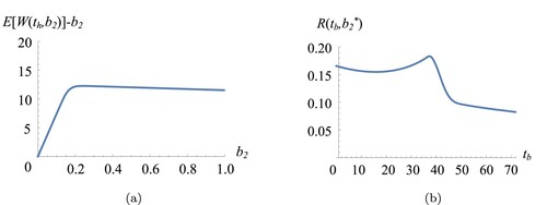
To visualise Proposition 4.3, Figure 2 presents two scenarios obtained from our case study. The solid line represents the base case obtained from industry data, and the dashed line represents a scenario where the batch has a stochastically lower time to enter the stationary phase. For these two batches, Figure 2 plots (i) the rate function of entering the stationary phase $\nu \left(m\right)$ over m; (ii) the cumulative distribution function $G\left(t\right|b_1)$ over t; (iii) the yield obtained from the second cultivation $\mathbb{E}\left[W\right(t_h,b_2\left)\right]-b_2$ over $b_2$; and (iv) the expected throughput $R(t_b,b_2^{\ast })$ over $t_b$. Observe from Figure 2 that the resulting expected yield from the second cultivation $\mathbb{E}\left[W\right(t_h,b_2\left)\right]-b_2$ and the expected throughput $R(t_b,b_2^{\ast })$ are lower for the high risk batch.

Figure 2. Plots of $\nu \left(m\right),G\left(t\right|b_1)$, $\mathbb{E}\left[W\right(t_h,b_2\left)\right]-b_2$ and $R(t_b,b_2^{\ast })$, for the industry base case (solid line), and a scenario with a higher risk of entering the stationary phase (dashed line).

Four line plots displaying (i) the rate function versus the biomass amount; (ii) the cumulative distribution function of entering the stationary phase versus time; (iii) the expected yield obtained from the second cultivation versus the starting biomass amount for the second cultivation; and (iv) the throughput function versus bleed–feed time. All four figures plot two specific cases using a solid and a dashed line, i.e. a base case which represents the industry case study (solid line), and the case when the risk of entering the stationary phase is higher (dashed line). The figures show that the high-risk case dominates the base case in the rate and cumulative distribution function plots whereas the base case dominates the high-risk case in the expected yield and throughput plots.

5. Case study

We present a case study from MSD in Boxmeer, the Netherlands. We use the case study to (i) demonstrate the room for improvement by the bleed–feed implementation and (ii) investigate the additional benefit of jointly optimising the bleed–feed time and the starting biomass amount for the second cultivation. For our numerical analysis, we identified a wide range of practically relevant configurations with our industry partners. We understand that the performance of fermentation processes varies for different cell cultures (i.e. viruses or bacteria), medium (i.e. different types and formulations) and equipment (i.e.bioreactor mechanism and size). Therefore, we present a comprehensive sensitivity analysis to generate managerial insights for the industry. First, we explain the data collection and present the base case (Section 5.1). Then we conduct numerical experiments on critical process parameters, such as biomass growth rate (Section 5.2), failure risks (Section 5.3) and setup duration (Section 5.4).

5.1. Data collection and the base case

In the case study, we use 3 years of fermentation data for a specific active ingredient of an animal drug. This data was obtained from various measurements performed by MSD. More specifically, the data consisted of two main data sets including: (i) fermentation information (e.g, initial biomass amount, end biomass amount, growth rate, etc.) and (ii) physicochemical parameters monitored through the fermentation (e.g. pH, temperature, oxygen levels, etc.) for each batch. The latter were in terms of plots, showing the process parameter versus time. Specific pattern changes in these plots were used to detect different growth phases during the fermentation. These plots were available in paper format and needed to be transformed into digital form manually. Then, the two data sets were combined into one master data file for determining the case study parameters.

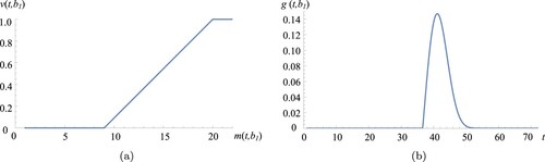
We establish the case study parameters as follows: the fermentation starts with $b_1=1$ gram biomass. The biomass growth rate is $\mu =0.06$ cell divisions per hour. The rate function is obtained from the data as explained in Appendix. Figure 3 depicts the rate function used in the base case and the corresponding probability density function for the time to enter stationary phase (given that $b_1=1$ g). Observe from Figure 3(a) that the critical biomass level is $m^{\prime }=9$ g. Due to the growth limiting factors (e.g.cell characteristics and media formulation) the biomass can reach at most H = 20 g. Finally, time to harvest a cultivation is $t_h=72$ h, and setup duration is s = 8 h. We refer this setting as the base case in our numerical analysis. We note that all parameters presented in this section are representative values to protect confidentiality.

Figure 3. The rate function used in the base case (a) and the corresponding probability density function (b). (a) The rate function $\nu \left(t|b_1\right)$ and (b) the corresponding probability density function, $g\left(t|b_1\right)$.

(a) A line graph displaying the rate function (i.e. rate of entering the stationary phase) versus the biomass amount for the base case setting. The -axis represents the biomass amount and the -axis denotes the rate. The rate is equal to 0 until 9 g biomass, and then linearly increases until 20 g. The rate is equal to 1 when the biomass amount is greater than 20 g. (b) A bell-shaped graph displaying the probability density function versus time. The -axis represents the time and the -axis denotes the probability density function.

To establish a benchmark and assess the potential benefits of our model, we consider the following strategies in our case study ³:

1. Current practice (CP) harvests the batch at the harvest time $t_h$ without implementing bleed–feed. The harvest time $t_h$ is exogenously prespecified by manufacturing protocols. This strategy represents the current industry practice, as bleed–feed is a novel technique and has not been implemented yet.

2. Naive Bleed–feed Policy (NBP) implements bleed–feed at critical biomass time $t^{\prime }$. Under this strategy, we assume that $b_2$ is fixed at $b_2=b_1$. We consider NBP because it is a simple and practically relevant heuristic, as Section 4 indicates that optimal bleed–feed time can be only at $t^{\prime }$ or later.

3. Bleed–feed optimisation (BO) maximises the expected throughput by finding the optimal bleed–feed time alone. Under this strategy, we assume that $b_2$ is fixed at $b_2=b_1$. This strategy aligns with the work of Koca et al. (2021).

4. Joint bleed–feed optimisation (JBO) corresponds to our renewal model (described in Section 3) and optimises both the bleed–feed time $t_b$ and the starting biomass amount for the second culture $b_2$ to maximise the expected throughput.

To assess the room for improvement with bleed–feed implementation, we compute the percentage improvement ($\mathrm{\%}I$) in the expected throughput that could have been achieved by NBP, BO and JBO instead of CP. We used Mathematica software to solve the numerical experiments.⁴

We present the results for the base case in Table 2. We observe that the expected throughput in CP is R = 0.156. It is optimal to bleed–feed at time $t_b^{\ast }=37.3$ for BO and $t_b^{\ast }=37.2$ for JBO. By optimising the bleed–feed time alone with BO, we can already achieve $13\mathrm{\%}$ improvement on the expected throughput. By jointly optimising the bleed–feed time and the replenishment amount with JBO, the percentage improvement increases to $17\mathrm{\%}$. We obtain that the optimal initial biomass amount for the second cultivation is $b_2^{\ast }=0.2$ g in JBO. Note that this $b_2^{\ast }$ value is less than $b_2=b_1=1$ g used in BO. This is because JBO considers the relationship between the starting biomass $b_2$ and the duration of the exponential growth phase, whereas BO omits this trade-off. We observe that the performance ($\mathrm{\%}I$) of NBP and BO is similar, yet NBP performs bleed–feed slightly earlier than BO.

Table 2. Base case results and the room for improvement on current practice.

CP	NBP			BO			JBO
R	$t^{\prime }$	$R\left(t^{\prime }\right)$	%I	$t_b^{\ast }$	$R\left(t_b^{\ast }\right)$	%I	$t_b^{\ast }$	$b_2^{\ast }$	$R(t_b^{\ast },b_2^{\ast })$	%I
0.156	36.6	0.176	12%	37.3	0.177	13%	37.2	0.2	0.183	17%

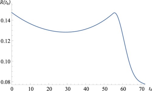
Figure 4 plots the expected throughput $R\left(t_b\right)$ as a function of the bleed–feed time $t_b$ under the BO strategy (i.e. for $b_2=b_1=1$ g). First, we observe from Figure 4 that the expected throughput $R\left(t_b\right)$ is not necessarily concave in $t_b$. However, we see that the throughput reaches its maximum at $t_b^{\ast }=37.3$, with one peak point. This behaviour illustrates the trade-off between the bleed–feed time and biomass yield. Bleed–feeding too early (before $t_b^{\ast }=37.3$) results in lower yield and throughput. Bleed–feeding too late (after $t_b^{\ast }=37.3$) causes a steep decrease in throughput as bleed–feed is more likely to fail.

Figure 4. Base case throughput $R\left(t_b\right)$ versus $t_b$ in BO strategy.

A line graph displaying the expected throughput as a function of the bleed–feed time (considering the base case under strategy BO). The expected throughput reaches its peak value of 0.177 at the bleed–feed time 37.3. This function has a convex shape before the peak and is decreasing after the peak.

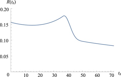
Figure 5 presents a surface plot showing the expected throughput $R(t_b,b_2)$ for JBO strategy as a function of bleed–feed time $t_b$ and the biomass amount $b_2$. We obtained Figure 5 by optimising $t_b$ and $b_2$ simultaneously (by solving the two-dimensional optimisation problem in Equation (5(5) $\begin{array}{rl}max& R(t_b,b_2)\\ \mathrm{s}.\mathrm{t}.& 0<b_2\le b_1,\\ & 0\le t_b\le t_h.\end{array}$(5) ). Note that reducing this joint optimisation problem into two sequential, one-dimensional optimisation problems would lead to the same results (as explained in Section 3.3). For illustration, Figure 6 shows $\mathbb{E}\left[W\right(t_h,b_2\left)\right]-b_2$ in $b_2$ (Figure 6a) and $R(t_b,b_2^{\ast })$ in $t_b$ (Figure 6 b), which are obtained by solving the reduced optimisation problems. We observe from Figures 5 and 6 that the expected throughput reaches its maximum at $b_2^{\ast }=0.2$ and $t_b^{\ast }=37.2$.

Figure 5. Surface plot depicting base case throughput $R(t_b,b_2)$ versus $t_b$ and $b_2$ in JBO strategy, when $t_b$ and $b_2$ are optimised simultaneously.

A 3D surface plot displaying the expected throughput as a function of the bleed–feed time and the initial biomass amount for the second cultivation. This 3D plot is depicted for the strategy JBO. The expected throughput reaches its maximum value of 0.183 when the bleed–feed time is 37.2 and the initial biomass amount is 0.2 g.

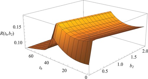
Figure 6. Reducing two-dimensional JBO into two sequential one-dimensional optimisation problems: (a) $\mathbb{E}\left[W\right(t_h,b_2)-b_2$ versus $b_2$ and (b) $R(t_b,b_2^{\ast })$ versus $t_b$ for $b_2^{\ast }$.

(a) A line graph displaying the expected yield as a function of the starting biomass amount after bleed–feed (under the base case). The -axis represents the starting biomass amount for the second cultivation, and the -axis denotes the expected yield obtained from the second cultivation. The expected yield increases steeply until 0.2 g biomass, after which it decreases slowly. (b) A line graph displaying the expected throughput as a function of the bleed–feed time (under the base case). The expected throughput reaches its peak value of 0.183 at the bleed–feed time 37.2, and has a convex shape before the peak.

We now investigate the behaviour of the objective function under $b_2$ and $t_b$. In Figure 6(a), the expected yield first increases in $b_2$ steeply and then decreases slowly. The underlying reason can be explained as follows: the optimal amount $b_2^{\ast }$ in JBO ensures that we can obtain the highest yield possible from the second cultivation by capturing the complex dynamics of cell growth (given biomass growth rate μ, the probability to enter stationary phase and the harvest time $t_h$). If we start with a lower biomass then $b_2^{\ast }$, the cell growth might not end before the prespecified harvest time $t_h$ in the second cultivation and we harvest with little yield. Hence, the expected yield increases sharply in $b_2$ until we reach $b_2^{\ast }$ in Figure 5(a). In contrast, when we start the second cultivation with more biomass then $b_2^{\ast }$, this does not necessarily imply that we produce high yield in the second cultivation as the growth is limited (due to the trade-off between starting biomass and duration of the exponential growth). When we start with higher biomass than $b_2^{\ast }$ in the second cultivation, this means that we extract less biomass from the first cultivation while the yield from second cultivation remains almost constant. Hence, the overall expected yield decreases so as the throughput. Consistent with our result from Section 4.1, Figure 6(a) shows that $\mathbb{E}\left[W\right(t_h,b_2\left)\right]-b_2$ is concave in $b_2$. In Figure 6(b), we observe a similar pattern for $R(t_b,b_2^{\ast })$ in $t_b$ (as in Figure 4) and hence omit the discussion. From practical point of view, these observations imply bleed–feeding too late and/or starting the second cultivation with too little biomass is worse off (in terms of expected throughput) than bleed–feeding too early and/or starting with too much biomass.

5.2. Sensitivity on biomass growth rate

Biomass growth rate μ can be different across cell cultures based on the biological characteristics (virus or bacteria), medium and equipment used. Hence, we considered the following scenarios for the biomass growth rate: (i) base case, $\mu =0.06$, (ii) slow growth, $\mu =\{0.04,0.045,0.05,0.055\}$, and (iii) fast growth, $\mu =\{0.065,0.07,0.075,0.08\}$. Table 3 presents these scenarios in the first column and reports the optimal expected throughput R, optimal bleed–feed times $t_b^{\ast }$ and the optimal amount $b_2^{\ast }$ to start the second cultivation under relevant strategies. Columns $\mathrm{\%}I$ show the percentage improvements in the expected throughput under the strategies NBP, BO and JBO compared to CP. Bold entries represent the base case.

Table 3. Sensitivity on the biomass growth rate μ.

		NBP			BO			JBO
μ	CP R	$t^{\prime }$	$R\left(t^{\prime }\right)$	$\mathrm{\%}I$	$t_b^{\ast }$	$R\left(t_b^{\ast }\right)$	$\mathrm{\%}I$	$t_b^{\ast }$	$b_2^{\ast }$	$R(t_b^{\ast },b_2^{\ast })$	$\mathrm{\%}I$
0.04	0.147	54.9	0.147	0%	0	0.147	0%	0	–	0.147	0%
0.045	0.150	48.8	0.155	4%	49.5	0.156	4%	49.4	0.6	0.158	6%
0.05	0.152	43.9	0.163	7%	44.6	0.163	7%	44.6	0.4	0.168	10%
0.055	0.154	39.9	0.170	10%	40.6	0.170	11%	40.6	0.3	0.176	14%
0.06	0.156	36.6	0.176	12%	37.3	0.177	13%	37.2	0.2	0.183	17%
0.065	0.158	33.8	0.182	15%	34.5	0.183	15%	34.4	0.2	0.190	20%
0.07	0.160	31.4	0.187	17%	32.1	0.188	17%	32.0	0.1	0.196	22%
0.075	0.162	29.3	0.192	18%	30.0	0.194	19%	29.9	0.1	0.202	24%
0.08	0.164	27.5	0.197	20%	28.1	0.198	21%	28.1	0.1	0.207	26%

We observe from Table 3 that as the growth rate μ increases, the throughput R increases in all strategies (since the expected yield increases for a fast-growing batch). With bleed–feed (in BO and JBO strategies), we see that the faster the biomass grows, the earlier the optimal bleed–feed time becomes. The reason is that a fast-growing batch consumes the medium faster and enters the stationary phase earlier. The system tends to bleed–feed earlier to avoid entering the stationary phase and losing the bleed–feed opportunity. Additionally, as growth rate μ increases, the optimal starting amount $b_2^{\ast }$ decreases. This is because of the relationship between the staring amount and the duration of the exponential growth phase, as explained in Section 1. Consistent with analytical results, NBP performs the bleed–feed slightly earlier than BO. However, we observe that the performance ($\mathrm{\%}I$) of NBP and BO is similar in all scenarios considered in Table 3.

As biomass grows faster, the biomass yield increases and the fermentation cycle time of the first cultivation decreases (because the optimal policy tends to bleed–feed earlier). Subsequently, throughput R and the improvement percentage $\mathrm{\%}I$ increase for both BO and JBO at higher growth rates μ. However, the increase in $\mathrm{\%}I$ decreases in μ. This behaviour is associated with the exponential growth behaviour of the biomass: for fast-growing cells, the exponential growth phase ends earlier and hence the optimal bleed–feed times (and fermentation cycle times) become closer between the scenarios. We also observe from Table 3 that the additional benefit obtained by joint optimisation JBO increases as the batch grows faster. The underlying intuition of this behaviour can be explained as follows. Recall that BO uses a heuristic that starts the second cultivation with the same amount as the first one, i.e. $b_2=b_1$. However, we observe from Table 3 that the optimal amount $b_2^{\ast }$ (suggested by JBO) is lower than $b_1$ (suggested by BO) and decreases in μ. Hence, the difference between $b_2^{\ast }$ and $b_1$ increases when the growth rate μ gets higher. For practitioners, these observations indicate bleed–feed (both BO and JBO strategies) have stronger business case for fast-growing batches, and the additional benefits provided by JBO become more pronounced as the growth rate μ increases.

Table 3 indicates that $t_b^{\ast }=0$ when $\mu =0.04$. This implies that it is optimal not to bleed–feed when the biomass growth rate is too small. To visualise this behaviour, Figure 7 plots the expected throughput $R\left(t_b\right)$ as a function of bleed–feed time $t_b$ under BO strategy when $\mu =0.04$. We observe from Figure 7 that the biomass grows so slowly that the system needs too much time until any significant biomass is obtained in the first cultivation. Thus it becomes optimal to produce only one batch without bleed–feed. We note that this result is consistent with our analysis in Section 4.1. For practitioners, these observations imply that bleed–feed is not an attractive option for slow growing cell cultures.

Figure 7. Throughput $R\left(t_b\right)$ versus bleed–feed time $t_b$ in BO strategy for slow growth ($\mu =0.04$).

A line graph displaying the expected throughput as a function of the bleed–feed time (for a slow growing batch under strategy BO). When the bleed–feed time is between 0 and 56, the expected throughput has a convex shape (i.e. it is first decreasing and then increasing), where the maximum throughput 0.147 is reached at time zero.

5.3. Sensitivity on the risk of entering the stationary phase

We now investigate the impact of the risk of entering the stationary phase on optimal throughput and bleed–feed policies.

5.3.1. Sensitivity on critical biomass level

Recall that the rate of transitioning to the stationary phase starts to be greater than zero when the biomass amount reaches the critical level $m^{\prime }$. In our sensitivity analysis, we considered the following scenarios for the critical biomass level: (i) base case, $m^{\prime }=9$ g, (ii) lower critical biomass level, $m^{\prime }=\{1,3,5,7\}$ g and (iii) higher critical biomass level, $m^{\prime }=\{11,13,15\}$ g. Table 4 presents these scenarios in the first column and reports the expected throughput R, optimal bleed–feed time $t_b^{\ast }$ and the optimal start amount $b_2^{\ast }$ for the second cultivation under relevant strategies. Bold entries represent the base case.

Table 4. Sensitivity on the critical biomass level $m^{\prime }$.

	CP	NBP			BO			JBO
$m^{\prime }$	R	$t^{\prime }$	$R\left(t^{\prime }\right)$	$\mathrm{\%}I$	$t_b^{\ast }$	$R\left(t_b^{\ast }\right)$	$\mathrm{\%}I$	$t_b^{\ast }$	$b_2^{\ast }$	$R(t_b^{\ast },b_2^{\ast })$	$\mathrm{\%}I$
1	0.040	0	0.040	0%	4.7	0.041	2%	1.4	0.1	0.051	28%
3	0.074	18.3	0.081	9%	20.5	0.082	10%	20.0	0.2	0.090	21%
5	0.104	26.8	0.115	11%	28.2	0.116	12%	28.0	0.2	0.124	19%
7	0.131	32.4	0.147	12%	33.4	0.148	13%	33.3	0.2	0.154	18%
9	0.156	36.6	0.176	12%	37.3	0.177	13%	37.2	0.2	0.183	17%
11	0.180	40.0	0.204	13%	40.4	0.205	13%	40.4	0.3	0.210	17%
13	0.203	42.7	0.230	13%	43.1	0.231	14%	43.1	0.3	0.236	17%
15	0.223	45.1	0.255	14%	45.3	0.255	14%	45.3	0.3	0.261	17%

In Table 4, we observe that the expected throughput R increases as $m^{\prime }$ increases for all strategies. We obtain this behaviour because, for high $m^{\prime }$, we can produce higher biomass amounts without failure risk (risk of entering the stationary phase). This leads to higher expected yield and throughput. The additional benefit obtained from JBO decreases as critical biomass level $m^{\prime }$ increases. The underlying reason can be explained as follows: recall that $b_2$ is fixed at $b_2=1$ g under BO. In JBO, $b_2^{\ast }$ is increasing in $m^{\prime }$ and getting closer to $b_2=1$. Thus BO and JBO perform similar as $m^{\prime }$ increases. We note that except from the scenario $m^{\prime }=1$, the improvement percentages of the scenarios are close for a given strategy ($\mathrm{\%}I$ ranges between 10–14% for BO and 17–21% for JBO). This is because the throughput already increases in $m^{\prime }$ under CP. Hence, practitioners should keep in mind that BO brings more benefit when $m^{\prime }$ is high, and JBO brings more benefit when $m^{\prime }$ is low, although both strategies improve the throughput as $m^{\prime }$ increases. Consistent with results from Section 4.1, Table 4 indicates that NBP implements the bleed–feed slightly earlier than BO and JBO. Nevertheless, $\mathrm{\%}I$ obtained from NBP and BO strategies are similar, especially for high-risk batches (i.e. higher $m^{\prime }$ values).

Table 4 shows that the optimal bleed–feed time $t_b^{\ast }$ increases in $m^{\prime }$. This is because the risk of entering the stationary phase starts later when the critical biomass level $m^{\prime }$ gets higher. Hence, the system can collect higher amounts of biomass without risking the bleed–feed. Also, observe that $b_2^{\ast }$ increases in $m^{\prime }$. The underlying intuition is related to the complex inter-dependency between $b_2^{\ast }$, $m^{\prime }$ and $t_b^{\ast }$. Notice that the optimal policy tends to bleed–feed earlier at lower values of $m^{\prime }$. This also implies that we reach lower biomass amounts at time $t_b^{\ast }$ when $m^{\prime }$ is low. However, we aim to obtain as much biomass as possible from both cultivations. To obtain more from the first cultivation (although $t_b^{\ast }$ is low), we tend to extract more biomass from the first cultivation during bleed–feed. For the second cultivation, this leads to lower starting amounts $b_2^{\ast }$ for lower $m^{\prime }$ values.

5.3.2. Sensitivity on maximum biomass level

The maximum biomass amount H that can be obtained from a cell culture could be finite because of limited cell viability. Hence, we investigate the following scenarios: (i) base case, H = 20 g, (ii) lower levels of maximum biomass, $H=\{12,15\}$ g and (iii) higher levels of maximum biomass, $H=\{25,30,35,40,45,50,55\}$ g. We refer to the cases with lower H as ‘high risk’ batches (as their risk of entering the stationary phase is higher). Table 5 presents the results.

Table 5. Sensitivity on maximum biomass that can be obtained H.

	CP	NP			BO			JBO
H	R	$t^{\prime }$	$R\left(t^{\prime }\right)$	$\mathrm{\%}I$	$t_b^{\ast }$	$R\left(t_b^{\ast }\right)$	$\mathrm{\%}I$	$t_b^{\ast }$	$b_2^{\ast }$	$R(t_b^{\ast },b_2^{\ast })$	$\mathrm{\%}I$
12	0.134	36.6	0.161	20%	36.8	0.161	20%	36.8	0.2	0.168	25%
15	0.144	36.6	0.167	16%	37.0	0.168	17%	37.0	0.2	0.175	21%
20	0.156	36.6	0.176	12%	37.3	0.177	13%	37.2	0.2	0.183	17%
25	0.167	36.6	0.183	10%	37.5	0.184	11%	37.5	0.3	0.190	14%
30	0.176	36.6	0.190	8%	37.7	0.191	8%	37.6	0.3	0.197	12%
35	0.185	36.6	0.195	6%	37.9	0.197	7%	37.8	0.3	0.203	10%
40	0.193	36.6	0.201	4%	38.1	0.203	5%	38.0	0.4	0.208	8%
45	0.201	36.6	0.206	3%	38.2	0.209	4%	38.1	0.4	0.213	6%
50	0.208	36.6	0.211	2%	38.4	0.214	3%	38.3	0.4	0.218	5%
55	0.215	36.6	0.216	0%	38.5	0.219	2%	38.4	0.4	0.223	4%

Observe from Table 5 that the throughput increases in H for all scenarios. The reason is that the expected yield increases when the batch can reach higher biomass values H. We also observe that $\mathrm{\%}I$ decreases both in BO and JBO as H increases. This is because the throughput R in CP is already high when H is high. Besides, the biomass yield obtained from the second cultivation when the bleed–feed is successful is similar to the expected yield obtained from the first cultivation under CP (as all scenarios have the same growth conditions for similar time duration). For these reasons, $\mathrm{\%}I$ is lower for higher H values. This indicates that the business case for bleed–feed is stronger when the maximum biomass level H is small (i.e. when cells have a low production capacity).

We observe from Table 5 that the optimal bleed–feed time $t_b^{\ast }$ increases as the maximum possible biomass amount H increases. The reason can be explained as follows: for higher H values, the risk of entering the stationary phase is lower. Hence, we can bleed–feed later without increasing the risk of failure. Observe also that $b_2^{\ast }$ increases as H gets higher under JBO. This is because when H is lower, a smaller amount of initial biomass $b_2$ would be sufficient to obtain the maximum possible yield from that batch. For practitioners these results indicate that both the bleed–feed time $t_b^{\ast }$ and the starting amount $b_2^{\ast }$ should be higher when H increases. Lastly, we observe from Table 5 that NBP and BO provide similar improvements $\mathrm{\%}I$, as their suggested bleed–feed times are close, especially for high-risk batches.

5.4. Sensitivity on setup duration

The setup time needed for cleaning the bioreactor and transferring the medium and the seed culture into the bioreactor can vary across different bioreactor sizes. Hence, we consider the following cases for the setup duration: (i) base case, s = 8 h, (ii) shorter setups, $s=\{0,2,4,6\}$ h and (iii) longer setups, $s=\{10,12,14\}$ h. These scenarios are shown in the first column in Table 6. The expected throughput, optimal bleed–feed time and the staring amount for the second cultivation are also presented in Table 6 for relevant strategies. Bold entries represent the base case.

Table 6. Sensitivity on setup duration s.

	CP	BO			JBO
s	R	$t_b^{\ast }$	$R\left(t_b^{\ast }\right)$	$\mathrm{\%}I$	$t_b^{\ast }$	$b_2^{\ast }$	$R(t_b^{\ast },b_2^{\ast })$	$\mathrm{\%}I$
0	0.174	37.3	0.190	9%	37.2	0.2	0.197	13%
2	0.169	37.3	0.186	10%	37.2	0.2	0.193	14%
4	0.165	37.3	0.183	11%	37.2	0.2	0.190	15%
6	0.160	37.3	0.180	12%	37.2	0.2	0.186	16%
8	0.156	37.3	0.177	13%	37.2	0.2	0.183	17%
10	0.153	37.3	0.174	14%	37.2	0.2	0.180	18%
12	0.149	37.3	0.171	15%	37.2	0.2	0.177	19%
14	0.145	37.3	0.168	16%	37.2	0.2	0.174	20%

In Table 6, we observe that $\mathrm{\%}I$ ranges between $\mathrm{\%}9$ and $\mathrm{\%}16$ for BO, and $\mathrm{\%}13$ and $\mathrm{\%}20$ for JBO when the setup duration changes from 0 to 14 h. In the extreme case where the bioreactor has no setup (s = 0), the benefit of bleed–feed is still $\mathrm{\%}9$ for BO and $\mathrm{\%}13$ for JBO. This insight is interesting because it means that the percentage improvement $\mathrm{\%}I$ obtained through bleed–feed is not only a result of producing higher biomass yield per single setup but also of decreased processing time with bleed–feed, i.e. fermentation processing time (excluding setup times) for two cultivations takes $(t_b+t_h)$ with bleed–feed and $(t_h+t_h)$ without bleed–feed (note that the harvest time $t_h\ge t_b$ because the batch is harvested in the stationary phase, whereas bleed–feed is performed in the exponential growth phase). Hence, the benefits of bleed–feed come from a combination of the reduced processing and setup times and increased levels of biomass production per setup.

Notice from Table 6 that expected throughput R decreases as setup duration s increases in all strategies. This is because the setup duration does not affect the expected yield but only prolongs the expected cycle length. For this reason, optimal bleed–feed time $t_b^{\ast }$ (both for BO and JBO) and the starting amount $b_2^{\ast }$ (for JBO) are robust to setup time s. In addition, we observe that the benefits ($\mathrm{\%}I$) of bleed–feed increase as the setup duration s increases (under both BO and JBO).

6. Conclusion

Setups are needed before a fermentation process to clean and sterilise the bioreactor. These setups are time-consuming as they can take up to 10 h (Sharma 2019). Therefore, increasing the fermentation throughput is a critical problem to improve efficiency. To address this problem, we consider a novel approach for eliminating bioreactor setups: bleed–feed.

Bleed–feed enables to skip intermediary bioreactor setups by replenishing some amount of the culture by fresh medium, instead of harvesting the batch. It is a novel method for prolonging the cell growth in batch fermentation. However, the timing of bleed–feed is important for a successful implementation. Bleed–feed can only be performed in the exponential growth phase of fermentation. As the duration of the exponential growth phase is random, there is a trade-off between implementing bleed–feed too soon versus too late. In addition, the starting biomass amount of the second cultivation (after bleed–feed) affects the expected fermentation yield and throughput. In this work, we formulate the critical trade-offs associated with bleed–feed decisions. We build a stochastic optimisation model using renewal reward theory and determine an optimal bleed–feed time and starting biomass amount to maximise the expected throughput. Our model links the biological dynamics of fermentation with operational trade-offs to support optimal decision-making.

We explore the structural properties of the optimisation problem. We generate insights on optimal policies and assess the impact of risks. Based on an industry case study obtained from MSD Animal Health, we present a comprehensive numerical analysis and analyse the potential impact of implementing bleed–feed on current practice. Our numerical analysis shows that bleed–feed can bring benefits. By jointly optimising the bleed–feed time and amount, our case study (base case) shows that the expected throughput can increase by $17\mathrm{\%}$ compared to current practice. We also observe that bleed–feed has a stronger business case for fast-growing cells, high risk cultures or long setups.

The applications of Operations Research (OR) methodologies to improve biomanufacturing efficiency have been limited. Our work illustrates how OR can complement life sciences to create impact. Future work could investigate the applications of our bleed–feed model in other industries such as food processing. As a limitation, our work assumes that sufficiently large production data is available to make inferences on fermentation dynamics. However, this might not necessarily hold for all biopharmaceutical research and development projects. Therefore, future studies could train machine learning models to support bleed–feed decisions under limited data. As another limitation, our model does not consider production planning and scheduling constraints, such as operator and equipment availability. As a future work, it would be interesting to expend the scope of our model to include resource limitations and planning constraints.

Disclosure statement

No potential conflict of interest was reported by the authors.

Additional information

Funding

This work was supported by Horizon 2020 Framework Programme [Marie Curie Fellowship] and nederlandse organisatie voor wetenschappelijk onderzoek [VENI Grant].

Notes on contributors

Yesim Koca

Yesim Koca is a Ph.D. student in the Department of Industrial Engineering and Innovation Sciences at Eindhoven University of Technology. Her research interests include applied statistics, and stochastic modelling and optimisation.

Tugce Martagan

Tugce Martagan is an assistant professor in the Department of Industrial Engineering and Innovation Sciences at Eindhoven University of Technology. She received her Ph.D. in Industrial Engineering from the University of Wisconsin-Madison. Her research interests include the design and optimisation of manufacturing systems.

Ivo Adan

Ivo Adan is a professor at the Department of Industrial Engineering of the Eindhoven University of Technology. His current research interests are in modelling, design and control of manufacturing systems, warehousing systems and transportation systems, and more specifically, in the analysis of multi-dimensional Markov processes and queueing models.

Notes

1 The harvest time for the second cultivation is prespecified by manufacturing protocols and cannot be changed.

2 The starting biomass amount of the second cultivation is controlled by adjusting the amount of biomass extracted from the first cultivation during bleed–feed.

3 Note that it is also possible to define another strategy where the starting amount is optimised alone by assuming a predefined bleed–feed time. For ease of exposition, we did not include this strategy in our numerical experiment (i.e. its performance was sensitive to the assumption on bleed–feed time and the results were not practically-relevant).

4 To evaluate JBO, we optimised the bleed–feed time $t_b$ and the replenishment amount $b_2$ simultaneously. Note that the reduced problem (i.e. solving two sequential, one-dimensional optimisation problems) would produce the same results, as described in Section 3.3.

Appendix. Establishing the transition rate function from industry data

We explain a procedure to obtain the rate function from industry data. Let $\nu \left(m\right)$ denote the rate of entering the stationary phase, and $F\left(m\right)$ denote the (long-run) fraction of batches that enter the stationary phase at a biomass of at most m, and $f\left(m\right)$ is the corresponding density, i.e. $f\left(m\right)=F^{\prime }\left(m\right)$. If Δ is a small time interval, then the probability that a batch will enter the stationary phase at biomass between m and $m(1+\mu \mathrm{\Delta })$ (recall that the growth is exponential), given that at time t the batch has m units biomass satisfies $f\left(m\right)\mu m\mathrm{\Delta }=\nu \left(m\right)\mathrm{\Delta }(1-F(m\left)\right).$Hence, $\frac{f\left(m\right)}{1-F\left(m\right)}=\frac{\nu \left(m\right)}{\mu m}.$The function $F\left(m\right)$ can be directly estimated from the industry data, m discretised with stepsize δ. If we then approximate $f\left(m\right)\approx F\left(\right(m+1\left)\delta \right)-F\left(m\delta \right)$, we obtain as estimate for the stationary phase function $\frac{F\left(\right(m+1\left)\delta \right)-F\left(m\delta \right)}{1-F\left(m\delta \right)}\approx \frac{\nu \left(m\delta \right)}{\mu m}$or rewritten, $\nu \left(m\delta \right)\approx \mu m\frac{F\left(\right(m+1\left)\delta \right)-F\left(m\delta \right)}{1-F\left(m\delta \right)}\mathrm{f}\mathrm{o}\mathrm{r}m=0,\delta ,2\delta \dots .$This rate function is used to establish the probability of entering the stationary phase, as explained in Section 3.2.1.

References

- Bei, X., X. Zhu, and D. W. Coit. 2019. “A Risk-averse Stochastic Program for Integrated System Design and Preventive Maintenance Planning.” European Journal of Operational Research 276 (2): 536–548.
- Boone, T., R. Ganeshan, Y. Guo, and J. K. Ord. 2000. “The Impact of Imperfect Processes on Production Run Times.” Decision Sciences 31 (4): 773–787.
- Çetinkaya, S., and C.-Y. Lee. 2000. “Stock Replenishment and Shipment Scheduling for Vendor-managed Inventory Systems.” Management Science 46 (2): 217–232.
- Chang, H.-C., and C.-H. Ho. 2010. “Exact Closed-form Solutions for ‘Optimal Inventory Model for Items with Imperfect Quality and Shortage Backordering’.” Omega 38 (3–4): 233–237.
- Chang, H. N., N.-J. Kim, J. Kang, C. M. Jeong, J.-D.-R. Choi, Q. Fei, B. J. Kim, S. Kwon, S. Y. L. Lee, and J. Kim. 2011. “Multi-stage High Cell Continuous Fermentation for High Productivity and Titer.” Bioprocess and Biosystems Engineering 34 (4): 419–431.
- Cherkaoui, H., K. T. Huynh, and A. Grall. 2018. “Quantitative Assessments of Performance and Robustness of Maintenance Policies for Stochastically Deteriorating Production Systems.” International Journal of Production Research 56 (3): 1089–1108.
- Colletti, P. F., Y. Goyal, A. M. Varman, X. Feng, B. Wu, and Y. J. Tang. 2011. “Evaluating Factors that Influence Microbial Synthesis Yields by Linear Regression with Numerical and Ordinal Variables.” Biotechnology and Bioengineering 108 (4): 893–901.
- Cunha, C., J. Glassey, G. Montague, S. Albert, and P. Mohan. 2002. “An Assessment of Seed Quality and Its Influence on Productivity Estimation in an Industrial Antibiotic Fermentation.” Biotechnology and Bioengineering 78 (6): 658–669.
- D'anjou, M. C., and A. J. Daugulis. 2001. “A Rational Approach to Improving Productivity in Recombinant Pichia pastoris Fermentation.” Biotechnology and Bioengineering 72 (1): 1–11.
- Doran, P. M. 1995. Bioprocess Engineering Principles. London: Elsevier.
- European Commission. 2020. “The Research Project Was One of the Three Finalists of 2020 MSCA2020.HR Awards. The Competition Was Among All Disciplines to Acknowledge the Most Influential Projects Under Horizon 2020 Program of European Commission.” https://msca2020.hr/msca-awards/.
- Handlogten, M. W., A. Lee-O'Brien, G. Roy, S. V. Levitskaya, R. Venkat, S. Singh, and S. Ahuja. 2018. “Intracellular Response to Process Optimization and Impact on Productivity and Product Aggregates for a High-titer CHO Cell Process.” Biotechnology and Bioengineering 115 (1): 126–138.
- IFORS News. 2020. “Innovative Applications of Operations Research: Reducing Costs and Lead Times in Biomanufacturing.” https://www.ifors.org/newsletter/ifors-news-march-2020.pdf.
- IMPACT. 2020. “Operational Research Improves Biomanufacturing Efficiency.” https://www.theorsociety.com/publications/magazines/impact-ma.
- Kachrimanidou, V., A. Vlysidis, N. Kopsahelis, and I. K. Kookos. 2020. “Increasing the Volumetric Productivity of Fermentative Ethanol Production Using a Fed-batch Vacuferm Process.” Biomass Conversion and Biorefinery 11 (2): 1–8.
- Kaminsky, P., and Y. Wang. 2015. “Analytical Models for Biopharmaceutical Operations and Supply Chain Management: a Survey of Research Literature.” Pharmaceutical Bioprocessing 3 (1): 61–73.
- Kapadi, M. D., and R. D. Gudi. 2004. “Optimal Control of Fed-batch Fermentation Involving Multiple Feeds Using Differential Evolution.” Process Biochemistry 39 (11): 1709–1721.
- Karamatsoukis, C., and E. Kyriakidis. 2009. “Optimal Maintenance of a Production-inventory System with Idle Periods.” European Journal of Operational Research 196 (2): 744–751.
- Koca, Y., T. Martagan, I. Adan, L. Maillart, and B. van Ravenstein. 2021. “Increasing Biomanufacturing Yield with Bleed-Feed: Optimal Policies and Insights.” Working paper. https://papers.ssrn.com/sol3/papers.cfm?abstract_id=3659907.
- Li, D., L. Qian, Q. Jin, and T. Tan. 2011. “Reinforcement Learning Control with Adaptive Gain for a Saccharomyces cerevisiae Fermentation Process.” Applied Soft Computing 11 (8): 4488–4495.
- Limon, Y., and A. Krishnamurthy. 2020. “Resource Allocation Strategies for Protein Purification Operations.” IISE Transactions 52 (9): 945–960.
- Maddah, B., and M. Y. Jaber. 2008. “Economic Order Quantity for Items with Imperfect Quality: Revisited.” International Journal of Production Economics 112 (2): 808–815.
- Martagan, T., A. Krishnamurthy, and C. T. Maravelias. 2016. “Optimal Condition-based Harvesting Policies for Biomanufacturing Operations with Failure Risks.” IIE Transactions 48 (5): 440–461.
- Mordor Intelligence. 2020. “Biopharmaceuticals Market -- Growth, Trends, and Forecasts (2020–2025).” Accessed 19 January 2021. https://www.mordorintelligence.com/industry-reports/global-bi.
- MSD. 2019. “Operations Research Improves Biomanufacturing Efficiency.” Accessed 25 June 2019. https://www.youtube.com/watch?v=79B7OBuvRkY&feature=youtu.be.
- Muldowney, M. 2018. “Continuous vs. Batch Production.” https://www.contractpharma.com/issues/2018-04-01/view_feature.
- Nakanishi, S. C., L. B. Soares, L. E. Biazi, V. M. Nascimento, A. C. Costa, G. J. M. Rocha, and J. L. Ienczak. 2017. “Fermentation Strategy for Second Generation Ethanol Production From Sugarcane Bagasse Hydrolyzate by Spathaspora passalidarum and Scheffersomyces stipitis.” Biotechnology and Bioengineering 114 (10): 2211–2221.
- Nederlandse Biotechnologische Vereniging. 2018. “Computers and Bioprocess Development.” Accessed 28 March 2018. https://nbv.kncv.nl/en/activities/nbv-detail-page/411/computers-bioprocess-development/about.
- Peroni, C. V., N. S. Kaisare, and J. H. Lee. 2005. “Optimal Control of a Fed-batch Bioreactor Using Simulation-based Approximate Dynamic Programming.” IEEE Transactions on Control Systems Technology 13 (5): 786–790.
- Rebaiaia, M. L., D. Ait-kadi, and A. Jamshidi. 2017. “Periodic Replacement Strategies: Optimality Conditions and Numerical Performance Comparisons.” International Journal of Production Research55 (23): 7135–7152.
- Ross, S. M. 1996. Stochastic Processes. 2nd ed. New York: Wiley.
- Sabri-Laghaie, K., and R. Noorossana. 2016. “Reliability and Maintenance Models for a Competing-risk System Subjected to Random Usage.” IEEE Transactions on Reliability 65 (3): 1271–1283.
- Sahling, F., and G. J. Hahn. 2019. “Dynamic Lot Sizing in Biopharmaceutical Manufacturing.” International Journal of Production Economics 207 (2): 96–106.
- Sharma, M. 2019. “Maximizing Biomanufacturing Productivity in Single-Use Applications.” https://www.medicaldesignbriefs.com/component/content/article/mdb/features/technology-leaders/35518.
- Villaverde, A. F., S. Bongard, K. Mauch, E. Balsa-Canto, and J. R. Banga. 2016. “Metabolic Engineering with Multi-objective Optimization of Kinetic Models.” Journal of Biotechnology 222 (3): 1–8.
- Walker, N. 2017. “Perfusion Appears to be Gaining Traction in Biopharma Manufacturing.” https://www.pharmasalmanac.com/articles/perfusion-appears-to–be-gaining-traction-in-biopharma-manufacturing.
- Wang, W.-B. 2000. “A Model to Determine the Optimal Critical Level and the Monitoring Intervals in Condition-based Maintenance.” International Journal of Production Research 38 (6): 1425–1436.
- Wang, Y., W. Sun, S. Zheng, Y. Zhang, and Y. Bao. 2019. “Genetic Engineering of Bacillus sp. and Fermentation Process Optimizing for Diacetyl Production.” Journal of Biotechnology 301: 2–10.
- Xie, W., B. Wang, C. Li, J. Auclair, and P. Baker. 2020. “Bayesian Network Based Risk and Sensitivity Analysis for Production Process Stability Control.” Preprint, Submitted September 10: 2019.
- Yang, Y., and M. Sha. 2019. “A Beginner's Guide to Bioprocess Modes–Batch, FedBatch, and Continuous Fermentation.” https://www.eppendorf.com/product-media/doc/en/763594/Ferment-Bioreactors_Application-Note_408_BioBLU-f-Single-Vessel_A-Beginner%E2%80%99s-Guide.
- Zeng, L., X. Deng, and J. Yang. 2018. “Constrained Gaussian Process with Application in Tissue-engineering Scaffold Biodegradation.” IISE Transactions 50 (5): 431–447.