Robust capacity planning for sterilisation department of a hospital

ABSTRACT

Sterile services departments are special units designed to perform sterilisation operations in an efficient way within a hospital. The delays in sterilisation services cause significant disruptions on surgery schedules and bed management. To prevent the delays, an upper time limit can be imposed on the time spent in the sterilisation services. In this paper, we propose a mathematical modelling approach for the optimum capacity planning of a sterilisation service unit considering the uncertainties in the sterilisation process. The model aims to find the optimum capacity on four tandem steps of the sterilisation whilst at the same time minimising the total cost and keeping the maximum time in the system below a limit. Assuming general distributions for service and interarrival times, an approximation structure based on robust optimisation is used to formulate the maximum time spent in the system. We analysed the structural property of the resulting model and found that the relaxed version of the model is convex. The real data from a large sterilisation services unit is used for computational experiments. The results indicated that the approximation fits well against the simulated maximum time in the system. Other experiments revealed that an upper limit of 7 hours for the sterilisation services balances the cost vs. robustness trade-off.

KEYWORDS:

• Stochastic programming
• robust optimisation
• sterilisation services
• queuing theory
• hospital operations

Introduction

The demand for healthcare services has been constantly increasing due to the aging population. Along with the need for decreasing costs, healthcare facilities are under pressure to plan their capacities more effectively. However, several complexities arise while planning the capacity of a healthcare facility. First, a healthcare system involves multiple stakeholders with competing interests such as those of administrative staff, medical staff, and public policy makers. In addition to that, the operations of a healthcare system involve various uncertainties that need to be taken into account. One of the most significant uncertainties in a healthcare system is the duration requiblack to treat a patient. Another layer of complexity within a healthcare system is the existence of multiple steps which both follow, and interact, one with the other.

Surgery suites are seen as the engines of hospitals since they are one of the most profitable healthcare services (Carey, Burgess, and Young 2011). Around 10 million operations are performed every year in England (NHS 2019), and forty percent of the overall revenue in the UK hospitals is generated by surgeries (Healthcare Financial Management Association (HFMA) 2005). On the other hand, the surgery suites account for the majority of hospitals' operational capacity (Macario et al. 1995), as they consume a significant amount of physical resources such as beds and equipment, as well as human resources with different levels of expertise.

Most surgical procedures involve a medical device or a surgical instrument in contact with patients' tissues or membranes. All this equipment and devices can lead to infection if not disinfected or sterilised correctly. The biological processes behind the infections and microorganisms invasions are understood much better thanks to the pioneering work of Louis Pasteur (Simpson, Núñez, and Almonacid 2012). This understanding eventually accelerated improvements of two crucial medical concepts: disinfection and sterilisation. Disinfection is ‘the process of eliminating or reducing harmful microorganisms from inanimate objects and surface’, while sterilisation is ‘the process of killing all microorganism’ (McKeen 2018). Within a hospital, the disinfection and sterilisation process is conducted at special facilities designed for this purpose which are called sterilisation units.

There are over 200 sterilisation units in England, and each one employs around 30 staff on average (National Health Services (NHS) 2021). These units are called as sterile services department (SSD). Some small hospitals in the UK do not have their own sterilisation unit and thus outsource the sterilisation to a large nearby hospital. The main reason for outsourcing is the high cost of these operations, especially due to the expensive, modern disinfection and sterilisation machines. Within an NHS hospital with an SSD, all used surgery kits are sent to the SSD in special transportation equipment.

An SSD usually comprises three areas: contaminated, decontaminated and sterilisation. Once the kits arrive in the contaminated area, the technicians scan the barcode of the surgery kit into the online tracking system. Then, the surgery kit is checked for each item, and the items that require pre-washing are processed by technicians. Next, they are placed in washer-disinfector (WD) machines which apply several stages of disinfection. When a cycle of the WD machine is completed, the disinfected kits are unloaded from the other side of the machine which is also in the decontaminated area. This area has strict sterilisation rules with special air conditioning and staff clothing. The staff in the decontaminated area check the surgery kits and employ special tests to ensure that the decontamination is performed perfectly. Then they wrap the kits with a special folding technique (Superior Health Council of Belgium 2017) and textile that has indication labels on it which change colour during the sterilisation process. The wrapped kits are then placed within the steam sterilisation machines (autoclaves) that sterile the kits in high temperatures. After the sterilisation machine completes its cycle, the kits are left in a cooling area or sent straight away back to the surgical departments where the kits came from.

If sterilisation processes take long to be completed, excessive quantities of surgery kits need to be stored in the operating theatre to prevent any shortage (Rappold et al. 2011). These stocks create certain costs such as holding cost, and thus, should be minimised (Ahmadi et al. 2019). On the other hand, lack of necessary equipment requires emergency solutions that lead to delays in patient treatment and potentially life-threatening cases. In fact, these delays create a knock-on effect due to the interconnectedness of a hospital's subsystems. For example, the delay in surgery schedules leads to disruption to the hospital's bed management system.

This paper is concerned with the capacity planning of an SSD. Due to the significant effect of an SSD on hospital operations, capacity planning of these units should be performed carefully. First, the time for the sterilisation process should be limited such that the surgery schedules are built in with enough confidence. To ensure a timely sterilisation process, the number of staff and machines in SSD should be increased. However, these resources are quite costly and inflexible, i.e. cannot be varied quickly. Therefore, finding the optimum number of staff and machines requires consideration of the uncertainties and complexities of the whole sterilisation process. Among these uncertainties, the arrival time of the surgery kits mostly affects the process, as the completion time of the surgeries is not deterministic. Another significant variation is observed in the processing time of the kits in the pre-wash and pre-sterilisation steps.

A confounding characteristic of the process is the existence of four queues following each other: pre-wash, wash-disinfection, pre-sterilisation check, and sterilisation. The time spent in these four tandem queues should be modelled to find the maximum time in system (TIS), i.e. the maximum time for a kit to be processed. For this purpose, queuing theory can be utilised. However, queuing theory can only provide approximate, not exact, formulations for TIS when the interarrival and service times do not follow exponential distributions, as in the sterilisation services. To overcome this complexity, we utilise an alternative approximation for the maximum TIS (MTIS) based on a combination of robust optimisation concepts with queuing theory.

This approximation is then incorporated within a mathematical optimisation model aimed at finding the optimum capacities for the four steps of the sterilisation process under budget and space limitations. The resulting formulation is a non-linear, integer programming model that is hard to solve with traditional techniques. We then analyse the structural property of this model and find that the model is convex. With this property, the problem can be optimally solved using commercial mixed-integer non-linear programming (MINLP) solvers.

The approach explained above is applied to the SSD of a large NHS hospital (UK National Health Service) that is about to go for a renewal of its capacity planning due to increased demand in recent years. The hospital consists of around 1000 beds, 26 operating theatres, and serves over a million people. The SSD of the hospital also provides outsourced services to a nearby private hospital. Using the data from the SSD, we design computational experiments to (i) investigate the performance of the MTIS approximation and (ii) to provide policy insights into the management of the SSD. To do (i), we develop a discrete-event simulation of the system, collect measures for TIS, and compare those with the approximation. For (ii), we test the impact of several possible scenarios on the results.

A summary of the contributions of this paper are:

1. Formulating a stochastic model of the SSD capacity planning problem,

2. Using an approximation for MTIS and investigating the structural properties of the resulting model,

3. Analysing the power of the approximation and generating useful policy insights through computational experiments.

The paper is organised as follows. The next section introduces the literature related to (i) capacity planning in healthcare, (ii) mathematical modelling of sterilisation services, and (iii) approximations for tandem queues' performance measures. Section 2 provides the problem description and underlying assumptions along with the optimisation model formulation. Section 3 presents the approximation for MTIS followed by the structural property of the resulting model. In Section 4, we introduce the design of experiments and results. Finally, Section 5 summarises the study and provides future research directions.

1. Related literature

Capacity planning is a major field of study in Operations Research and generally refers to more effective planning of the resources to satisfy the varying demand. Capacity planning has been performed for various healthcare facilities such as intensive care units (Gallivan et al. 2002; Harper, Powell, and Williams 2010), inpatient clinics (Gnanlet and Gilland 2009; Creemers and Lambrecht 2009), and hospitals (Utley et al. 2003; Kim et al. 2006; Kortbeek et al. 2012). Important factors on capacity planning studies are the uncertainties in demand, service times, staff availability, medical results, etc. Several approaches can be utilised to deal with these uncertainties, e.g. sensitivity analysis can be used as a post-optimisation tool to investigate the impact of possible scenarios. Alternatively, the expected values of the uncertain parameters may be utilised within the mathematical formulation. However, this would lead to an optimum solution for only one realisation of uncertainty (that is the expected value) and might give underperforming results for other realizations.

Another approach widely utilised for the capacity planning of healthcare services is queuing theory; readers are referred to Fomundam and Herrmann (2007) for a review. Queuing theory is a mathematical field of the study aiming to find performance measures of a queuing system. As an example, built-in queuing formulas can be utilised to find the capacity of appointment-driven health centres aiming to meet certain performance targets (Creemers and Lambrecht 2009). Hulshof et al. (2013) also use queuing formulas to compute the optimum number of patients to be served in elective patient admission and resource allocation for hospitals with uncertain treatment paths and number of arrivals. They consider several queues with time-dependent resource levels. Similarly, Cochran and Roche (Cochran and Roche 2009) utilise queuing theory to investigate the impact of various capacity design alternatives in a hospital emergency department. The main disadvantage of queuing theory is that most of the built-in formulations for the queue's performance measures are non-linear and require the arrival and service processes to follow certain distributions such as exponential.

For the cases where the queuing formulations are not available or tractable, simulation modelling is a viable alternative. Simulation is a very useful tool to analyse complex healthcare systems, but can only be used to find approximate solutions. This method is utilised heavily for healthcare capacity planning problems. Harper, Powell, and Williams (2010) model the operations in an intensive care unit with a discrete-event simulation model. Then, the data generated by the simulation model are given to the optimisation model which computes the optimum number of nurses. De Angelis, Felici, and Impelluso (2003) apply simulation optimisation to find the optimum capacity of a transfusion centre minimising the cost while at the same time achieving a fixed maximum waiting time. The operations of a blood collection unit are modelled by a discrete-event simulation by Alfonso et al. (2013). Finally, Di Mascolo and Gouin (2013) develop a generic simulation model of a sterilisation unit to support the decision-making of the unit.

The rest of this section provides a brief review of mathematical models for supporting the decision-making related to surgery kits and sterilisation units. A significant observation is that the literature for surgery kits or sterilisation units is scarce. Ahmadi et al. (2019) provide a literature review of inventory management models of surgical devices, while another review considering all material logistics within a hospital is provided in Volland et al. (2017). The models reviewed in these papers aim to answer questions such as how many surgical kits should be ordered or what should be the reorder and stock levels considering holding, storage and/or usage costs and space limitations. For example, Diamant et al. (2018) aim to find the best stock levels of reusable surgical devices for different sterilisation practices. Another branch of study related to surgical kits is the logistics of surgery material (van de Klundert, Muls, and Schadd 2008). These studies aim to find the right location of the sterilisation services within the hospital so that costs are reduced. Surgery kits are also considered within surgery scheduling studies such as in Coban (2020). This study combines the scheduling of the multi-room surgery suite and the reusable medical devices. However, the author assumes a fixed capacity for sterilisation machines. Finally, the literature related to disposable medical items can be considered as relevant. For example, Cardoen, Beliën, and Vanhoucke (2015) develop mathematical modelling to support the configuration and reconfiguration of sterile packs composed of multiple disposable medical items.

The closest paper to ours is that of Ozturk, Begen, and Zaric (2014) in which the authors aim to find the best schedule of surgery kits for WD machines minimising the makespan of washing operations. They develop a branch-and-bound algorithm to solve the resulting mixed-integer linear programming model. This work is then extended with the additional objective of minimising the flow time of washing machines (Ozturk 2020). The author utilises a partial 2-approximation to find the Pareto set. A similar paper to Ozturk, Begen, and Zaric (2014) is that of Rossi, Puppato, and Lanzetta (2013) who develop a job-shop scheduling model to assign surgery kits to WD and sterilisation machines during a day. The main difference between these papers and ours is the problem description. We aim to find the optimum capacities in several steps of a sterilisation process, whereas those studies aim to schedule specific surgery kits to the WD machines. Thus, they also do not take into account any queueing. This difference is due to the consideration of different SSDs with different operating rules.

As another related branch of study, we present a review of papers focusing on the use of approximations for tandem queues with general service and arrival time distributions. Tu and Chen (2009) aim to find the right capacity of machines in a G/G/m (general distribution for interarrival and service times) queuing network existing in a wafer production line with constraints on the number of items delayed. They use an approximation for the average waiting time. Since this approximation only works for continuous server capacity, they apply an error-minimising technique to find the appropriate integer server levels. Tu and Chen (2011) also utilise the same approximation for capacity planning in the wafer production. The main difference between this study and ours is on the use of a different performance indicator; we focus on MTIS while they focus on average waiting time in the queue. Therefore, the resulting approximations are essentially different from each other.

The robust approximation for time-based queue indicators is also used in Gökalp, Gülpınar, and Vinh Doan (2019). In this paper, the authors develop a stochastic programming model to find the optimum capacity of a stem-cell donation centre. They utilise an approximation of the maximum waiting time during the donation search process based on robust optimisation and queuing. The uncertainties are modelled with scenarios while the resulting mixed-integer linear model is solved with a commercial solver. As a differentiating factor to ours, they consider a single queue within the donation centre.

2. Problem description and formulation

This section first provides the details of the problem and then presents the mathematical model.

2.1. Problem description

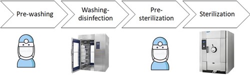
We consider the capacity planning of an SSD within a large NHS tertiary hospital. We assume that the SSD is designed from scratch.The sterilisation services are conducted in four main steps: pre-washing, disinfection-washing, checking and wrapping (also called as pre-sterilisation), and drying and sterilisation. The duration spent in these steps is stochastic. The first step requires the staff to check the used surgery kits for any missing/damaged items and conduct pre-washing for some of the items, taking around half an hour on average. The second step involves the use of special WD machines that runs for around 45 minutes in each cycle. In the third step, the staff check the washed items for any damage or improper sterilisation and pack them with special wrapping textile, taking around an hour on average. The final step requires using sterilisation machines that are also called autoclaves and takes around an hour. A representation of the process with indicators of the resources used in each step is shown in Figure 1. Note that the staff in step 1 and 3 are not the same.

Figure 1. A schematic representation of the whole sterilisation process with respective resources. Four symbols in order; the first, and third representing the resources, the other two are machines used in the SSD. One box above each symbol, with the text inside showing the label of that sterilisation step.

The kits are served in a first-come first served (FCFS) manner in this department which operates 24 hours in a day. The surgery kits should be sterilised and got ready for use as soon as possible to minimise the disruptions to surgery schedules. These disruptions would affect patients' health and cause further disruptions to surgery schedules and ward bed management. The SSD aims to find the optimum staff and machine levels to minimise total cost of these resources. Besides, the space required by these resources should be lower than the available space.

2.2. Problem formulation

Each step of the sterilisation service is denoted with $i\in \{1,\dots ,I\}$, where I is the total number of steps. The capacity at step i is denoted with $x_i$. The unit fixed cost of capacity in step i is represented with $c_i$. The management puts a limit on MTIS for the whole service which is denoted with $W^l$. We represent whole system-wide MTIS, that is the time a kit spends in the whole process, with a single variable, $W\left(\mathbf{x}\right)$ (where $\mathbf{x}$ is the vector of $x_1,\dots ,x_I$). The space requirement of each unit capacity in step i is represented with $g_i$, while total available space to the department is S.

The main uncertainties in the problem are the variation in the interarrival times of the kits to the department and the time spent in each step. The arrival rate at each step is the same, since all kits follow the same procedure, and is represented with λ. The standard deviation in arrival times is denoted with ${\sigma }^a$. The service rate in step i is represented with ${\mu }_i$, while the standard deviation in service times is denoted with ${\sigma }_i^s$. Note that ${\sigma }_i^s$ is low for steps 2 and 4, i.e. disinfection-washing and drying and sterilisation, since these involve machines with relatively stable cycle times.

Several assumptions are made during the modelling of the process. These assumptions can be summarised as follows:

• We assume that the service and arrival times are independent of each other.

• We only consider the operations for the small/mid size surgical equipment. The department serves the sterilisation of large medical equipment as well, such as endoscopy devices. However, these services are provided in separate small subsections of the department, and thus, not considered here.

• The arrival rate is lower on the night shift due to a reduction in the number of operations. Here, we consider the arrival rate during the day shift which is the one with a higher TIS, and thus should be constrained.

• Note that TIS does not include the transportation of the kits from/to the surgical rooms, and to/from the sterilisation department which are not under the SSD's control.

A summary of the model notation can be found in Table 1.

Table 1. Model notation.

Notation	Description
Indices
i	Process steps $i=1,\dots ,I$.
Parameters
S	Total available space.
$W^l$	Limit on MTIS.
$g_i$	Space requirement of one unit of capacity in step i.
$c_i$	Cost of one unit of capacity in step i.
λ	Arrival rate to the sterilisation department.
${\sigma }^a$	Standard deviation of the interarrival times to the sterilisation department.
${\mu }_i$	Service rate in step i.
${\sigma }_i^s$	Service time standard deviation in step i.
Variables (Decisions)
$x_i$	Number of resources in step i.

Each step operates as an FCFS queue with multiple servers. The traffic intensity condition requires the total service rate to be higher than the total arrival rate in a queue, i.e. $x_i{\mu }_i>\lambda$. The total space required by the resources, $\sum _i{g}_i{x}_i$, is constrained by S. The objective function minimises the total cost that can be formulated as $\sum _i{c}_i{x}_i$. The model can be written as follows: (1) $\begin{array}{rl}\underset{x_i}{min}& \sum _i{c}_i{x}_i,\end{array}$(1) (2) $\begin{array}{rl}\mathrm{s}\mathrm{u}\mathrm{b}\mathrm{j}\mathrm{e}\mathrm{c}\mathrm{t}\mathrm{t}\mathrm{o}& x_i{\mu }_i\ge \lambda ,\mathrm{\forall }i\in \{1,\dots ,I\},\end{array}$(2) (3) $\begin{array}{rl}& W\left(\mathbf{x}\right)\le W^l,\end{array}$(3) (4) $\begin{array}{rl}& \sum _i{g}_i{x}_i\le S,\end{array}$(4) (5) $\begin{array}{rl}& x_i\in {\mathbb{Z}}^{+},\mathrm{\forall }i\in \{1,\dots ,I\}.\end{array}$(5) Note that this model requires to formulate MTIS of all steps which corresponds to finding the waiting time in the queue of each step i as well as the service time spent for that service. Since the arrival times of the kits in the department and the time spent in each step are uncertain factors, both the waiting times in the queues and the service times vary for each kit. Modelling each kit arriving in the department and for each possible scenario of the uncertainty realizations would result in a computationally large and intractable model. Therefore, we utilise alternative approaches based on robust optimisation and queuing theory.

3. Approximation of maximum time in system

MTIS can be approximated by various methods based on queuing theory only (Gupta and Osogami 2011). However, these approximations do not perform well if the arrival process does not follow a Poisson distribution (i.e. the interarrival times do not follow an exponential distribution) (Bandi and Bertsimas 2012). To provide a better approximation of MTIS for those cases, Bandi and Bertsimas (2012) and Bandi, Bertsimas, and Youssef (2018) suggest utilising robust optimisation concepts, assuming that the arrival and service times are independent and identically distributed (i.i.d.) random parameters following an unknown distribution with fixed number of servers and tandem FCFS queues. Below, we present an overview of their approach and then its application to our model.

Let us consider I tandem queues where each one is a FCFS queue for step i with $x_i$ number of servers. Interarrival and service times of kits $k=1,\dots ,K_i$ arriving to service i are represented by $T_k$ and $Y_k$, respectively. We define the uncertainty sets $U_i^{arrv}$ and $U_i^{serv}$ where random variables $T_k$ and $Y_k$, respectively, belong to. Note that the departure process from service i−1 represents the arrival process to queue i for $i=2,\dots ,I$. Bandi, Bertsimas, and Youssef (2018) show that the departure process from queue i for $i=1,\dots ,I$ belongs to the uncertainty set $U_1^{arrv}$ for the original arrival process, i.e. $U_1^{arrv}=U_i^{arrv}$ for $i=2,\dots ,I$.

The structure of these uncertainty sets is inspired from the central limit theorem that asserts asymptotic results for a large set of i.i.d. random variables: the sum of n random variables with mean $\overline{\xi }$ and standard deviation σ would have a normal distribution with mean $n\overline{\xi }$ standard deviation $\sigma \sqrt{n}$. Then, representing the sum of these random variables with M, probability that $M-n\overline{\xi }\le 2\sigma \sqrt{n}$ would be equal to 95%. Applying this general concept to the random variables of service times in each step i, we obtain $\sum _{k=1}^{K_i}{Y}_k-K_i/{\mu }_i\le {\mathrm{\Gamma }}_i^s{\sigma }_i^s\sqrt{K_i}$, while for the interarrival times, we obtain $\sum _{k=1}^{K_i}{T}_k-K_i/\lambda \le {\mathrm{\Gamma }}^a{\sigma }^a\sqrt{K_i}$. In these formulations, ${\mathrm{\Gamma }}_i^s$ and ${\mathrm{\Gamma }}^a$ resemble the z-value of the confidence level, and thus can be set to 2 or 3 which indicates that 95% or 99.75% of possible random variables are covered with the inequality, respectively. In other words, ${\mathrm{\Gamma }}^a$ and ${\mathrm{\Gamma }}_i^s$, that define the conservativeness of the model against the uncertainties of interarrival and service times, respectively, can be adjusted to determine the sizes of these uncertainty sets. As the values of the parameters ${\mathrm{\Gamma }}^a$ and ${\mathrm{\Gamma }}_i^s$ increase, the conservativeness level of the model rises.

The reader is referred to Bandi and Bertsimas (2012) and references therein for further details regarding the motivation of the uncertainty set structures as well as the general robust optimisation approach.

The uncertainty set $U_i^{arrv}$ for interarrival times $T_k$ of kits $k=1,\dots ,K_i$ is defined as follows: (6) $\begin{array}{rl}{U}_i^{arrv}& =\left\{\right(T_1,T_2,\dots ,T_{K_i})|\frac{|\sum _{k=m+1}^{K_i}{T}_k-\frac{K_i-m}{\lambda }|}{\sqrt{K_i-m}}\\ & \le {\mathrm{\Gamma }}^a{\sigma }^a,\mathrm{\forall }m\le m_0\},\end{array}$(6) where $1/{\lambda }_i=1/\lambda$ is the expected interarrival time, and $K_i-m$ represents the sample sizes used in the summation of random variables, i.e. m is the intermediate parameter used in the calculation of the sample sizes. The idea here is that, for various samples (with sample sizes of $K_i-m$, where m ranges between 0 and $m_0$) of $T_k$, the above inequality involving ${\mathrm{\Gamma }}^a$ in (6(6) $\begin{array}{rl}{U}_i^{arrv}& =\left\{\right(T_1,T_2,\dots ,T_{K_i})|\frac{|\sum _{k=m+1}^{K_i}{T}_k-\frac{K_i-m}{\lambda }|}{\sqrt{K_i-m}}\\ & \le {\mathrm{\Gamma }}^a{\sigma }^a,\mathrm{\forall }m\le m_0\},\end{array}$(6) ) would still be valid. Note that the sample size $K_i-m$ should be larger than 30 for the central limit theorem to hold, therefore a typical value for $m_0$ is $m_0=K_i-30$ (Bandi and Bertsimas 2012).

For the service times, we first define $e_i=\lfloor K_i/x_i\rfloor$ which is an approximate measure for the average number of kits processed by one server. Then, the jobs are partitioned into the sets $L_j=\{l\le K_i:\lfloor (l-1)/x_i\rfloor =j\}$ for $j=0,\dots ,e_i$. Let $l_j\in L_j$ denote the index of a job from $L_j$, for $j=0,\dots ,e_i$. The uncertainty set $U_i^{serv}$ for service times $Y_k$ of service requests $k=1,\dots ,K_i$ in step i is defined as (7) $\begin{array}{rl}{\displaystyle U_i^{serv}}& =\{\sum _{j\in \mathcal{J}}{Y}_{l_j}-\frac{|\mathcal{J}|}{{\mu }_i}\\ & \le {\mathrm{\Gamma }}_i^s{\sigma }_i^s\sqrt{|\mathcal{J}|},\mathrm{\forall }{l}_j\in L_j,j\in \mathcal{J}\subseteq \{0,\dots ,e_i\}\},\end{array}$(7) where $1/{\mu }_i$ is the expected service time. Notice that the uncertainty set in (7(7) $\begin{array}{rl}{\displaystyle U_i^{serv}}& =\{\sum _{j\in \mathcal{J}}{Y}_{l_j}-\frac{|\mathcal{J}|}{{\mu }_i}\\ & \le {\mathrm{\Gamma }}_i^s{\sigma }_i^s\sqrt{|\mathcal{J}|},\mathrm{\forall }{l}_j\in L_j,j\in \mathcal{J}\subseteq \{0,\dots ,e_i\}\},\end{array}$(7) ) consists of a set of service times that satisfy a number of constraints arrived at by applying the central limit theorem separately for each server.

Here, the central limit theorem (CLT) is used as the basis for forming the uncertainty sets, which is where belong the uncertain parameters, the interarrival times between kits and service times. Since the MTIS is a measure that would require to consider all the kits arriving to the system, not for a specified small time period where a handful of the kits would pass through the system, the interarrival and service times of a large number of kits have to be considered. This would mean that the sample size of our uncertain parameters is much larger than 30, which motivates the use of CLT to construct the uncertainty sets.

Given uncertainty sets $U_i^{arrv}$ and $U_i^{serv}$ (defined for random interarrival and service times of a stable multi-server queuing system), an upper-bound on MTIS, $W\left(x_i\right)$, is defined as $\overline{W}\left(\mathbf{x}\right)$, where $\mathbf{x}$ is the vector of all decision variables $x_i$ for $i=1,\dots ,I$. Assuming that every queue has the same utilisation, i.e. $\frac{\lambda }{{\mu }_i{x}_i}=\rho$, and service rate, ${\mu }_i=\mu$ for all $i=1,\dots ,I$, Bandi, Bertsimas, and Youssef (2018) formulate the upper bound of the total TIS (sum over all queues) in I tandem queues with m servers in each queue i as: (8) $\begin{array}{r}\overline{W}\left(\mathbf{x}\right)=\frac{\lambda {\mathrm{\Gamma }}^2}{4(m(1-\rho ))}+I/\mu +\sum _{i=1}^I{\mathrm{\Gamma }}_i^s{\sigma }_i^s,\end{array}$(8) where, $\mathrm{\Gamma }=\sqrt{m}{\mathrm{\Gamma }}^a{\sigma }^a+{\mathrm{\Gamma }}^m$, and, ${\mathrm{\Gamma }}^m=\sqrt{\sum _{i=1}^I({\mathrm{\Gamma }}_i^s{\sigma }_i^s{)}^2}$. Note that the approximation does not consider the queues independently, but provides an overall system-wide MTIS, except for variations in the service times. The formulation is arrived after a series of computations based on classical queuing theory concepts. The reader is referred to Bandi, Bertsimas, and Youssef (2018) for the proof and the details of parameter estimation. The overall quality of the approximation depends on the distributions of the interarrival and service times. According to Bandi, Bertsimas, and Youssef (2018), considering Pareto arrivals and exponential service times, the approximation is within 10% of the simulated waiting times and is even smaller (within 5%) as the average utilisation of the servers becomes higher.

However, note that we do not assume the same utilisation rate, service rate and number of servers in the queues. Thus, based on Bandi, Bertsimas, and Youssef (2015), we modify the formulation (8(8) $\begin{array}{r}\overline{W}\left(\mathbf{x}\right)=\frac{\lambda {\mathrm{\Gamma }}^2}{4(m(1-\rho ))}+I/\mu +\sum _{i=1}^I{\mathrm{\Gamma }}_i^s{\sigma }_i^s,\end{array}$(8) ) and approximate the upper bound of the total TIS as: (9) $\begin{array}{r}W\le \sum _i[\frac{\lambda ({\mathrm{\Gamma }}^a{\sigma }^a+\frac{{\mathrm{\Gamma }}_i^s{\sigma }_i^s}{\sqrt{x_i}}{)}^2}{4(1-\frac{\lambda }{{\mu }_i{x}_i})}+1/{\mu }_i+{\mathrm{\Gamma }}_i^s{\sigma }_i^s],\end{array}$(9) while the details of the computation are presented in Appendix. The differences between (8(8) $\begin{array}{r}\overline{W}\left(\mathbf{x}\right)=\frac{\lambda {\mathrm{\Gamma }}^2}{4(m(1-\rho ))}+I/\mu +\sum _{i=1}^I{\mathrm{\Gamma }}_i^s{\sigma }_i^s,\end{array}$(8) ) and (9(9) $\begin{array}{r}W\le \sum _i[\frac{\lambda ({\mathrm{\Gamma }}^a{\sigma }^a+\frac{{\mathrm{\Gamma }}_i^s{\sigma }_i^s}{\sqrt{x_i}}{)}^2}{4(1-\frac{\lambda }{{\mu }_i{x}_i})}+1/{\mu }_i+{\mathrm{\Gamma }}_i^s{\sigma }_i^s],\end{array}$(9) ) are (i) the use of separate utilisation rate over the queues instead of a single utilisation rate and (ii) replacing the single service rate μ with ${\mu }_i$. The impact of these modifications is examined in the computational experiments (Section 4) by modelling the process with discrete-event simulation. With this approximation, the model can be rewritten as:

(10) $\begin{array}{r}\begin{array}{rl}min& \sum _i{c}_i{x}_i\\ \mathrm{s}.\mathrm{t}.& \left(2\right),\left(4\right),\left(5\right),\\ & \sum _i[\frac{\lambda {({\mathrm{\Gamma }}^a{\sigma }^a+\frac{{\mathrm{\Gamma }}_i^s{\sigma }_i^s}{\sqrt{x_i}})}^2}{4(1-\frac{\lambda }{{\mu }_i{x}_i})}+1/{\mu }_i+{\mathrm{\Gamma }}_i^s{\sigma }_i^s]\le W^l.\end{array}\end{array}$(10) Note that MTIS approximation is a non-linear function of the decision variables. Therefore, this model cannot be solved with well-established mixed-integer linear programming algorithms such as branch-and-bound. In the next section, we further examine the structural property of the model, especially the convexity, to identify the right solution approach.

3.1. Structural property

In this section, we analyse the structural property of the model by relaxing the integrality condition of the decision variables, i.e. (5(5) $\begin{array}{rl}& x_i\in {\mathbb{Z}}^{+},\mathrm{\forall }i\in \{1,\dots ,I\}.\end{array}$(5) ). Note that MTIS approximation (9(9) $\begin{array}{r}W\le \sum _i[\frac{\lambda ({\mathrm{\Gamma }}^a{\sigma }^a+\frac{{\mathrm{\Gamma }}_i^s{\sigma }_i^s}{\sqrt{x_i}}{)}^2}{4(1-\frac{\lambda }{{\mu }_i{x}_i})}+1/{\mu }_i+{\mathrm{\Gamma }}_i^s{\sigma }_i^s],\end{array}$(9) ) is not linear even for continuous decision variables. However, if the relaxed model is convex, we can solve it to optimality, i.e. the global optimum can be found. To check whether it is convex or not, we need to derive the Hessian matrix of the function; let's denote the matrix with H that can be defined as:

$H=\left[\begin{array}{cccc}{\displaystyle \frac{{\mathrm{\partial }}^{2}f(\cdot )}{\mathrm{\partial }{x}_1^2}}& {\displaystyle \frac{{\mathrm{\partial }}^{2}f(\cdot )}{\mathrm{\partial }{x}_1\mathrm{\partial }{x}_2}}& {\displaystyle \frac{{\mathrm{\partial }}^{2}f(\cdot )}{\mathrm{\partial }{x}_1\mathrm{\partial }{x}_3}}& {\displaystyle \frac{{\mathrm{\partial }}^{2}f(\cdot )}{\mathrm{\partial }{x}_1\mathrm{\partial }{x}_4}}\\ {\displaystyle \frac{{\mathrm{\partial }}^{2}f(\cdot )}{\mathrm{\partial }{x}_2\mathrm{\partial }{x}_1}}& {\displaystyle \frac{{\mathrm{\partial }}^{2}f(\cdot )}{\mathrm{\partial }{x}_2^2}}& {\displaystyle \frac{{\mathrm{\partial }}^{2}f(\cdot )}{\mathrm{\partial }{x}_2\mathrm{\partial }{x}_3}}& {\displaystyle \frac{{\mathrm{\partial }}^{2}f(\cdot )}{\mathrm{\partial }{x}_2\mathrm{\partial }{x}_4}}\\ {\displaystyle \frac{{\mathrm{\partial }}^{2}f(\cdot )}{\mathrm{\partial }{x}_3\mathrm{\partial }{x}_1}}& {\displaystyle \frac{{\mathrm{\partial }}^{2}f(\cdot )}{\mathrm{\partial }{x}_3\mathrm{\partial }{x}_2}}& {\displaystyle \frac{{\mathrm{\partial }}^{2}f(\cdot )}{\mathrm{\partial }{x}_3^2}}& {\displaystyle \frac{{\mathrm{\partial }}^{2}f(\cdot )}{\mathrm{\partial }{x}_3\mathrm{\partial }{x}_4}}\\ {\displaystyle \frac{{\mathrm{\partial }}^{2}f(\cdot )}{\mathrm{\partial }{x}_4\mathrm{\partial }{x}_1}}& {\displaystyle \frac{{\mathrm{\partial }}^{2}f(\cdot )}{\mathrm{\partial }{x}_4\mathrm{\partial }{x}_2}}& {\displaystyle \frac{{\mathrm{\partial }}^{2}f(\cdot )}{\mathrm{\partial }{x}_4\mathrm{\partial }{x}_3}}& {\displaystyle \frac{{\mathrm{\partial }}^{2}f(\cdot )}{\mathrm{\partial }{x}_4^2}}\end{array}\right],$where $f(\cdot )$ represents (9(9) $\begin{array}{r}W\le \sum _i[\frac{\lambda ({\mathrm{\Gamma }}^a{\sigma }^a+\frac{{\mathrm{\Gamma }}_i^s{\sigma }_i^s}{\sqrt{x_i}}{)}^2}{4(1-\frac{\lambda }{{\mu }_i{x}_i})}+1/{\mu }_i+{\mathrm{\Gamma }}_i^s{\sigma }_i^s],\end{array}$(9) ). For $f(\cdot )$ to be convex, the leading principal minors of H should be positive. Representing $k^{th}$ leading principal minor with $D_k$, they are formulated as: $D_1=\frac{{\mathrm{\partial }}^{2}f(\cdot )}{\mathrm{\partial }{x}_1^2}$, $\begin{array}{rl}{D}_2& =\left|\begin{array}{cc}{\displaystyle \frac{{\mathrm{\partial }}^{2}f(\cdot )}{\mathrm{\partial }{x}_1^2}}& {\displaystyle \frac{{\mathrm{\partial }}^{2}f(\cdot )}{\mathrm{\partial }{x}_1\mathrm{\partial }{x}_2}}\\ {\displaystyle \frac{{\mathrm{\partial }}^{2}f(\cdot )}{\mathrm{\partial }{x}_2\mathrm{\partial }{x}_1}}& {\displaystyle \frac{{\mathrm{\partial }}^{2}f(\cdot )}{\mathrm{\partial }{x}_2^2}}\end{array}\right|,\\ D_3& =\left|\begin{array}{cccc}{\displaystyle \frac{{\mathrm{\partial }}^{2}f(\cdot )}{\mathrm{\partial }{x}_1^2}}& {\displaystyle \frac{{\mathrm{\partial }}^{2}f(\cdot )}{\mathrm{\partial }{x}_1\mathrm{\partial }{x}_2}}& {\displaystyle \frac{{\mathrm{\partial }}^{2}f(\cdot )}{\mathrm{\partial }{x}_1\mathrm{\partial }{x}_3}}& \\ {\displaystyle \frac{{\mathrm{\partial }}^{2}f(\cdot )}{\mathrm{\partial }{x}_2\mathrm{\partial }{x}_1}}& {\displaystyle \frac{{\mathrm{\partial }}^{2}f(\cdot )}{\mathrm{\partial }{x}_2^2}}& {\displaystyle \frac{{\mathrm{\partial }}^{2}f(\cdot )}{\mathrm{\partial }{x}_2\mathrm{\partial }{x}_3}}\\ {\displaystyle \frac{{\mathrm{\partial }}^{2}f(\cdot )}{\mathrm{\partial }{x}_3\mathrm{\partial }{x}_1}}& {\displaystyle \frac{{\mathrm{\partial }}^{2}f(\cdot )}{\mathrm{\partial }{x}_3\mathrm{\partial }{x}_2}}& {\displaystyle \frac{{\mathrm{\partial }}^{2}f(\cdot )}{\mathrm{\partial }{x}_3^2}}\end{array}\right|,D_4=\left|\begin{array}{c}H\end{array}\right|.\end{array}$Our analysis showed that $D_1$ is always positive for all parameter levels of $\lambda ,{\mathrm{\Gamma }}_a,{\mathrm{\Gamma }}_s^i,{\mu }_i$. However, since the resulting formulation is quite large, it is not presented here. Also, the other principal minors become exhaustively complicated and thus are not presented here. More details regarding this analysis can be found in the online supplementary folder. Our analysis showed that they are positive for the feasible set of $x_i$ values. Therefore, constraint (10(10) $\begin{array}{r}\begin{array}{rl}min& \sum _i{c}_i{x}_i\\ \mathrm{s}.\mathrm{t}.& \left(2\right),\left(4\right),\left(5\right),\\ & \sum _i[\frac{\lambda {({\mathrm{\Gamma }}^a{\sigma }^a+\frac{{\mathrm{\Gamma }}_i^s{\sigma }_i^s}{\sqrt{x_i}})}^2}{4(1-\frac{\lambda }{{\mu }_i{x}_i})}+1/{\mu }_i+{\mathrm{\Gamma }}_i^s{\sigma }_i^s]\le W^l.\end{array}\end{array}$(10) ) is convex for the feasible set of continuous decision variables.

4. Computational experiments

This section aims to (i) analyse the performance of the MTIS approximation and (ii) provide policy suggestions to the decision-makers. First, we present the input data used for the experiments. All the experiments are conducted in Intel Core i7-6700K CPU @ 4.00 Ghz with 32 GB memory and x64 based processor.

4.1. Design of experiments and input data

The input data are estimated by the experts from the SSD of a large NHS tertiary hospital in the Midlands region of the UK. The fixed cost of the sterilisation (autoclave) machines ranges between $\mathcal{L}40-58$ K (Priorclave 2020). The fixed cost of the WD machines ranges between $\mathcal{L}15-20$ K (Bimedis 2020; Zauba 2020). These machines also require some variable costs like maintenance, water, energy, and reusables. In this case, the objective of the SSD management is the minimisation of the initial setup cost, and as such only included the purchase cost of the machines as well as the variable running costs. However, a more detailed costing analysis can certainly be done if required by the SSD management. The cost of staff in steps 1 and 3 are computed based on their monthly salaries assuming 3 years planning period. The length of the planning period is set based on the estimations of duration where the capacity would stay fixed. Table 2 shows the data used for the experiments.

Table 2. Input data for experiments.

Parameter	Level
$c_i$: Unit cost ($\mathcal{L}$) of resources in step i	[80 K, 50 K, 90 K, 110 K]
λ: Arrival rate per hour	6
${\mu }_i$: Service rate per hour in step i	[2, 1.3, 1, 1]
${\sigma }_i^s$: Service time variation in step i	[0.35, 0.1, 0.2, 0.05]
$W^l:$ Upper limit for total time in system.	7 hrs.

Since the arrival data of the kits are not available to us, we simulate the arrival of the surgery kits based on an exponential distribution with the rate shown in Table 2. Then, based on Bandi and Bertsimas (2012), we set the arrival variation as ${\mathrm{\Gamma }}^a,{\mathrm{\Gamma }}_i^s=2$. We apply the same procedure to the service times assuming that they follow a normal distribution. The motivation for using a normal distribution is based on the opinion of the experts who work for the SSD and thus have insights regarding the distribution of the task durations. We have also supported the assumption of the normal distribution by observing the system. The observed data, although limited, fitted a normal distribution more closely than other possible distributions such as exponential. Although step 2 and 4 consist of machines, they sometimes experience some glitches on their operating systems, which results in minor delays on the running times (usually the machines themselves resolve these issues quickly). To represent these delays, we have assumed quite low standard deviations of the running times.

Since the problem is convex in the continuous version, some local MINLP (mixed-integer Non-linear Programming) solvers can find the global optimum for the original formulation with integer decision variables. For this purpose, we use the Bonmin solver in GAMS that is known to provide the exact optimum for the MINLP problems that are found to be convex in the continuous version (please see GAMS (2021) for more details). Besides, to ensure that the local solver obtains the global solution, we also solve the problem with a global solver, Couenne implemented in Julia language (Julia Language 2021). In other words, the local solver is used to support the convexity claim, and when both the local and global solvers give the same solution, this suggests that the problem is indeed convex. Also, by using both solvers, we are able to cross-validate the solution.

GAMS offers a computing environment where the mathematical model is written in a language similar to Java or C++. Julia is a similar type of program that can be run from a terminal. In both software, the preferred solver, e.g. Bonmin or Couenne, can be specified along with the mathematical model. The BONMIN solver in GAMS uses branch-and-bound, branch-and-cut and outer approximation algorithms. Couenne also utilises branch-and-bound algorithms along with linearisation, bound reduction, and branching methods to find the global optimum on mixed-integer non-linear programming models.

Our experiments show that the global and local solvers find the same solution for different instances, confirming that the local solver obtains the global optimum. The computational time is a couple of seconds in both solvers.

To investigate the performance of the TIS approximation, we also develop a discrete-event simulation model of the process, explained in Section 2.1, using ARENA software (Rockwell Automation 2021). The capacities obtained by the optimisation model are given as the inputs to the simulation model, while the rest of the parameters are the same as in Table 2. The simulation model, with a time unit of an hour, is run for 500 iterations while each iteration simulates 5 days to obtain a large enough sample. Finally, the TIS of each kit in the simulation is collected, the maximum of these TIS in each iteration is identified, and 95% confidence interval (CI) of these maximum TIS is compared with the upper-bound of TIS computed by the approximation (9(9) $\begin{array}{r}W\le \sum _i[\frac{\lambda ({\mathrm{\Gamma }}^a{\sigma }^a+\frac{{\mathrm{\Gamma }}_i^s{\sigma }_i^s}{\sqrt{x_i}}{)}^2}{4(1-\frac{\lambda }{{\mu }_i{x}_i})}+1/{\mu }_i+{\mathrm{\Gamma }}_i^s{\sigma }_i^s],\end{array}$(9) ). The main reason for comparing 95% CI with the approximation is to achieve an approximate measure from the simulated TIS values such that we could have a meaningful comparison between the simulation and mathematical approximation.

Next, we first present the results for the base case and then perform a sensitivity analysis to provide policy suggestions.

4.2. Results

Table 3 shows the results for the base case obtained with GAMS (local solver) for the original version of the problem (i.e. with integrality constraints). The same results are obtained with the global solver, supporting that the relaxed problem (continuous version) is convex.

Table 3. Base results.

Cost	327
Steps	1	2	3	4
Capacities (number of servers)	9	10	11	10
Utilizations	0.37	0.49	0.6	0.63

In terms of capacities, measured as staff in steps 1 and 3, and machines for steps 2 and 4, we see that the highest capacity, with respect to the service rate, is required in step 1, though the service is the fastest in that step. The main reason behind this counter-intuitive result lies in the service variations: step 1 has a considerably higher service variation than other steps.

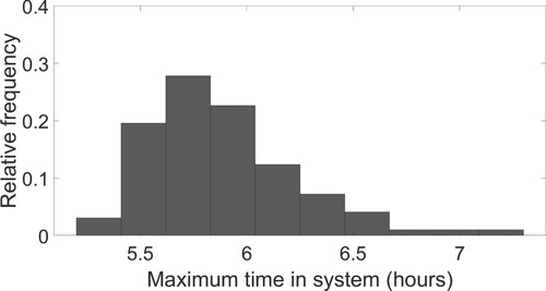
Figures 2 and 3, respectively, show the histograms of TIS of the kits and the maximums of TIS (in each iteration) obtained in the simulation model. The 95% confidence level of the maximum TIS's from the simulation model is 6.85 that is very close to the upper-bound of TIS in the optimisation model. The differences between these two levels is due to the fact that (i) the approximation does not guarantee to provide the exact point estimate, and (ii) the simulation is also an approximation to the reality.

Figure 2. Histogram of the simulated TIS. Histogram presenting the frequency of a certain TIS value among the simulation results.

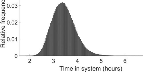
Figure 3. Histogram of the simulated MTIS. Histogram presenting the frequency of a certain MTIS value among the simulation results.

In the simulation model, the utilizations of the servers are 0.37, 0.49, 0.57, 0.61 which are also very close to the utilizations from the optimisation model. The comparison of the simulation and optimisation results indicates that the approximation structure used for MTIS performs fairly well.

4.2.1. Performance of approximation

We additionally analyse the performance of the approximation for different cases where the model parameters are varied from their base values. Specifically, three different cases are developed by changing the levels of several parameters to a different, but still realistic level, and the optimisation is run again. Particularly, the upper waiting time limit is set to 8 and 6 hours, respectively in the cases 1 and 2 (while case 3 has the base value of 7 hours limit). The main reasons for changing this parameter are (i) its significant impact on the capacity solutions and (ii) being the main parameter defining the value of the MTIS approximation computed through the optimisation. For the final case, additionally, the arrival rate, and therefore the (arrival time) standard deviation, are also set to different values than their default ones such that we can examine the impact of changing two parameters at the same time. The respective input data and the capacities are then given as inputs to the simulation model and the resulting MTIS are reported. The results, showing the 95% CI of the MTIS computed by the simulation as well as the changes made in the cases (compared to the base case), are presented in Table 4. The difference between the approximation and simulation (shown as ‘gap’ in the table) are 2.3%, 3.3% and 2%, respectively, in cases 1, 2, and 3. In all three cases, the waiting time computed based on the approximation is very close to the simulation results.

Table 4. Performance of the approximation on different cases.

Case	Changes made	95% MTIS from simulation
1	$W^l=8$	7.81 (2.3% gap)
2	$W^l=6$	5.8 (3.3% gap)
3	$\lambda =10({\sigma }^a=0.2)$	7.15 (2% gap)

4.3. Sensitivity analysis

This section aims to examine the impact of model parameters on the results as well as providing policy insights. For this purpose, we investigate the impact of the following parameters on the results: (i) the upper limit of TIS, (ii) arrival rate, (iii) arrival variation, (iv) service variation, and lastly, (v) more efficient machines.

4.3.1. Effect of upper limit of time in system

The most significant policy parameter in the problem is the upper limit on TIS because this parameter affects the surgical scheduling, and thus, the bed management. Therefore, the upper limit should be selected carefully and as low as possible to minimise any disruptions to the surgery-based operations of the hospital. We investigate its impact on the results by solving the optimisation model for a wide range of the parameter's value. A smaller limit may be preferred by the management to minimise the disruptions in the surgical operations, while a larger limit is less costly for the department.

For limits smaller than 6 hours, the problem becomes infeasible, whereas when the limit is above 13 hours, the results do not change. Therefore, Figure 4 only presents the results where the upper limit is between 6 and 13 hours.

Figure 4. Minimum cost obtained in different upper limits (hours) for TIS. A line plot where the x-axis ranges from 6 to 13 hours while the cost in y-axis ranges from around $\mathcal{L}$150 to $\mathcal{L}$1000.

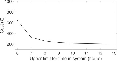
When the limit is higher than 8 hours, the cost is not affected significantly. On the other hand, when the limit is lower than 7 hours, the cost changes substantially, i.e. more than 200% for a reduction of limit from 7 to 6 hours. Based on these results, we observe that a limit of 7 hours balances the cost and robustness: increasing the limit above 7 hours does not decrease the cost much while decreasing the limit further from 7 to 6 hours results in a significant rise in the cost.

4.3.2. Effect of conservativeness rate

A higher rate of ${\mathrm{\Gamma }}^a$ corresponds to a more conservative model, taking more of the possible interarrival times into account. Note that when ${\mathrm{\Gamma }}^a=0$, the approximation is for the average TIS, not for MTIS. On the other hand, ${\mathrm{\Gamma }}^a=6$ covers almost all possible interarrival times (Bandi and Bertsimas 2012). Figure 5 shows the capacities as well as total cost obtained by the optimisation model for a plausible range of ${\mathrm{\Gamma }}^a$. The model becomes infeasible for ${\mathrm{\Gamma }}^a\ge 4$.

Figure 5. Minimum cost and capacities of sterilisation steps for various levels of arrival variation parameter. Three blocks and four line plots where x-axis represents the arrival variability levels of 1, 2, and 3. The first y-axis contains the cost that ranges between $\mathcal{L}$0 and $\mathcal{L}$1000, and the second y-axis contains the capacity levels between 0 and 40.

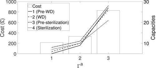
As expected, a more conservative model results in a higher cost due to larger capacities. However, we observe that the capacities are affected differently from the increase in the conservativeness. The largest capacity increase is observed in step 1 ( pre-sterilisation) which has the largest service variation. On the other hand, the capacity of step 4 (sterilization) is affected minimally. This is possibly due to the high cost of step 4 resources. In other words, increasing other steps' capacities is more cost-efficient than increasing that of step 4.

We see that the cost increase is larger as the conservativeness is increased; the change in the cost from ${\mathrm{\Gamma }}^a=1$ to ${\mathrm{\Gamma }}^a=2$ is much lower than that from ${\mathrm{\Gamma }}^a=2$ to ${\mathrm{\Gamma }}^a=3$. Thus, we can say that increasing the conservativeness level more than ${\mathrm{\Gamma }}^a=3$, already covering almost all of the uncertainty sets, does not add much but increases the cost significantly. In other words, increasing this parameter more than 3 is not suggested in terms of any trade-off between cost and conservativeness.

4.3.3. Effect of arrival rate

As mentioned before, total demand for the sterilisation department includes the surgery kits from a nearby private hospital. In this experiment, we aim to compute the change in the cost with different demand levels and provide decision support to the SSD management. For this purpose, we run the optimisation model for a plausible range of the arrival rate and present the cost and total capacity in Figure 6. We do not provide the capacities of steps separately, since they follow the same pattern as does the total capacity.

Figure 6. Minimum cost and total capacities of sterilisation steps for various levels of arrival rate. Several blocks and a line plot where x-axis represents the arrival rate between 4 and 9. The first y-axis contains the cost that ranges between $\mathcal{L}$300 and $\mathcal{L}$440, and the second y-axis contains the capacity levels between 35 and 50.

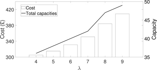
As expected, when the arrival rate is increased, the cost and total capacity increase almost linearly. Furthermore, total capacity and the cost increases by 34% and 25%, respectively, when the arrival rate doubles (from $\lambda =4$ to $\lambda =8$). This may be interpreted as resembling ‘economies of scale’. The policy implication of this result is that if the department sets the outsourcing price linearly dependent on the demand, then the department's profit increases. In other words, more contractual service is beneficial for the department.

4.3.4. Effect of service time variation

As shown in Section 4.2, the service time variation has a significant impact on the results. The service time variations in steps 2 and 4 are quite small due to the use of machines. However, steps 1 and 3 are mainly performed by technicians and prone to variation due to different requirements of the surgery kits. In this test, we examine the impact of service time variation on steps 1 and 3 on the results. Specifically, we assume two scenarios: the service time variation of steps 1 and 3 being (i) decreased to 0.1, and (ii) increased to 1. Case (i) can be achieved with enhanced automation in the manual operations. On the other hand, case (ii) is possible with the introduction of more complex surgical equipment in the hospital. Figure 7 shows the cost and capacities of steps in case (i) and case (ii), labelled as ‘low’ and ‘high’, respectively. Note that the capacities of some steps coincide in the base and low variation cases, and thus are not visible.

Figure 7. Minimum cost and capacities of sterilisation steps in different levels of service variations of steps 1 & 3. Three blocks and four different types of pointers in three different service variation levels. The first y-axis contains the cost that ranges between $\mathcal{L}$0–1000, and the second y-axis contains the capacity levels between 0 and 50.

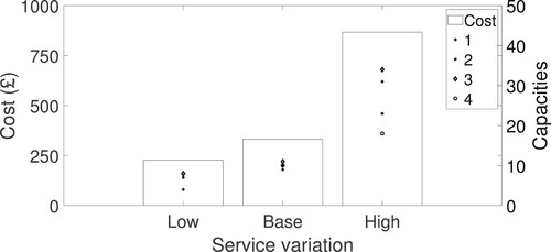
The results show that increasing the service variation causes a significant change in the cost while decreasing them does not. Similar to the arrival variation, the capacity of step 4 is more robust to the changes in the service time variation. Again, the most dramatic change happens in step 1 which has the highest original service time variation.

At the strategic level, the results indicate that further automation may not bring so much cost saving (unless they also reduce the service times), so should be performed with a detailed analysis of costs vs. benefits. Besides, the introduction of new complex surgery kits should be performed with caution since they can increase the service time variations.

4.3.5. Effect of machine efficiency

There is a continuous improvement in the efficiency of sterilisation and WD machines. We examine two related cases regarding the installation of more efficient machines in the department. The capacities are presented in Figure 8. The first case resembles the use of a more efficient but expensive WD model by the department. This scenario is inspired by the current debates in the department management on whether buying a more recent model would improve the department's performance. In this scenario, we assume that the unit capacity cost and service rate, i.e. average number of kits processed within one time unit, of step 2 are increased, respectively, by 50%. The service time variation is kept the same.

Figure 8. Capacities of sterilisation steps for WD and sterilisation machines with different efficiency and cost. Three x-axis ticks and four different coloured blocks for each x-axis tick, while the y-axis contains capacities ranging from 0 and 15.

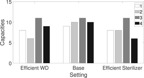
Similarly, the second case assumes that more efficient but expensive (50% as in the first scenario) sterilisation machines (step 4) are installed. Total costs of the scenarios are very close to that of the base case (within ± £3 of the base case cost), and thus, not presented here.

When a more efficient steriliser machine is used, the number of these machines, as well as pre-WD staff (step 1), and WD machines, are decreased since the efficiency is higher. Similarly, the results show that when a more efficient WD is utilised, the capacity of WD machines, as well as pre-WD and the sterilisation machines, are decreased. A policy recommendation based on these results is that the department can replace the existing machines with more efficient but expensive ones without disrupting the budget and MTIS performance.

5. Conclusions

Although mostly overlooked and isolated, sterilisation services have a crucial impact on the smooth running of the hospital operations. Delays with sterilisation cause disruptions to the surgery schedule and bed management. Thus, one way of preventing such delays is putting a maximum limit on the time spent for sterilisation. To achieve such a target, the capacities of the sterilisation steps may need to be adjusted. This paper proposes a mathematical model for capacity planning of an SSD operating under a maximum time limit target. Each step of the sterilisation service is modelled as queues with multiple servers and general interarrival and service time distributions. Since the queuing theory cannot provide efficient approximation formulations for MTIS, we utilise a novel approach combining robust optimisation and queuing theory. With this approximation, the model becomes an MINLP formulation that is hard to solve with established integer programming techniques. Next, we examine the structural property of the model and find that the model is indeed convex in the relaxed version. This property allows us to use a local MINLP solver that is known to provide the global optimum for MINLP problems that are convex in their relaxed version.

To examine the performance of the MTIS approximation and support their decision-making, we use the data estimated from the SSD of a large tertiary hospital in the UK. The experiment showed that the approximation performs reasonably well on estimating MTIS. The insights obtained from the rest of the experiments can be summarised as follows: (i) an upper limit of 7 hours for MTIS balances the cost vs. conservativeness trade-off, (ii) increasing the model conservativeness further than ${\mathrm{\Gamma }}^a=3$ is not beneficial, (iii) the department would better set the outsourcing prices linearly dependent on the demand, (iv) the automation of manual services (step 1 and 3) may not bring a significant cost saving unless the service times are also reduced, and (v) more efficient machines may not necessarily result in a lower cost. The study can be extended in the future by considering different combinations of different machine models in the WD and sterilisation steps. This extension may require the use of combinatorial optimisation approaches since convexity may not be achieved anymore. Also, the service times need to be estimated by simulating all possible combinations of different machine types. The work can also be expanded by assuming that the SSD management keeps some of the current sterilisation and WD machines which would require updating the cost function. One of the limitations of this work is the lack of real historical data for individual kit arrivals to the SSD. Once these data become available, the study can be extended to incorporate these. The work can also be extended to include the transportation of the kits to and from the SSD which would require to consider the transportation and collection times in the model.

Disclosure statement

No potential conflict of interest was reported by the author(s).

Data availability statement

The data that support the findings of this study are available from the corresponding author, [EG], upon reasonable request.

Additional information

Notes on contributors

Elvan Gökalp

Elvan Gökalp is a Lecturer (Assistant Professor) in the Information, Decisions & Operations division of the School of Management at the University of Bath. She obtained her PhD in Operational Research from Warwick Business School in the University of Warwick on 2017, where she also worked as a post-doctoral fellow until 2019. She completed MSc. in Management Science at London School of Economics on 2013. She obtained her BSc. from Bogazici University, Industrial Engineering department in 2012. Her research is mainly centered around decision-making under uncertainty in various fields such as healthcare and sustainable development.

Ece Sanci

Ece Sanci is a Lecturer (Assistant Professor) in the Information, Decisions & Operations division of the School of Management at the University of Bath. She received her Ph.D. in Industrial and Operations Engineering in 2019 from the University of Michigan, Ann Arbor. She received her B.S. and M.S. in Industrial Engineering in 2013 and 2015 from the Middle East Technical University (METU) in Ankara. Her research focuses on decision-making under uncertainty with applications in disaster relief management and supply chain risk management.

Appendix

Representing the maximum waiting time in service i with $W_i$, total worst-case waiting time in the system is limited by the sum of these MTIS as: (A1) $\begin{array}{r}W\le \sum _i{W}_i.\end{array}$(A1) In other words, the maximum time in the queuing network can be approximated by decomposing the network into individual queues (Bandi, Bertsimas, and Youssef 2015). Based on the formulations in Bandi, Bertsimas, and Youssef (2018) (Theorem 2, p. 15), $W_i$ can be reformulated as: (A2) $\begin{array}{r}{W}_i=\frac{\lambda {({\mathrm{\Gamma }}^a{\sigma }^a+\frac{{\mathrm{\Gamma }}_i^s{\sigma }_i^s}{\sqrt{x_i}})}^2}{4(1-\frac{\lambda }{{\mu }_i{x}_i})}+1/{\mu }_i+{\mathrm{\Gamma }}_i^s{\sigma }_i^s\end{array}$(A2) Thus, the overall MTIS can be approximated as: (A3) $\begin{array}{r}W\le \sum _i[\frac{\lambda {({\mathrm{\Gamma }}^a{\sigma }^a+\frac{{\mathrm{\Gamma }}_i^s{\sigma }_i^s}{\sqrt{x_i}})}^2}{4(1-\frac{\lambda }{{\mu }_i{x}_i})}+1/{\mu }_i+{\mathrm{\Gamma }}_i^s{\sigma }_i^s]\end{array}$(A3)

References

- Ahmadi, Ehsan, Dale T. Masel, Ashley Y. Metcalf, and Kristin Schuller. 2019. “Inventory Management of Surgical Supplies and Sterile Instruments in Hospitals: A Literature Review.” Health Systems 8 (2): 134–151.
- Alfonso, Edgar, Xiaolan Xie, Vincent Augusto, and Olivier Garraud. 2013. “Modelling and Simulation of Blood Collection Systems: Improvement of Human Resources Allocation for Better Cost-Effectiveness and Reduction of Candidate Donor Abandonment.” Vox Sanguinis 104 (3): 225–233.
- Bandi, Chaithanya, and Dimitris Bertsimas. 2012. “Tractable Stochastic Analysis in High Dimensions Via Robust Optimization.” Mathematical Programming 134: 23–70.
- Bandi, Chaithanya, Dimitris Bertsimas, and Nataly Youssef. 2015. “Robust Queueing Theory.” Operations Research 63 (3): 676–700.
- Bandi, Chaithanya, Dimitris Bertsimas, and Nataly Youssef. 2018. “Robust Transient Analysis of Multi-Server Queueing Systems and Feed-Forward Networks.” Queueing Systems 89 (3-4): 351–413.
- Bimedis. 2020. “Prices for Washer-Disinfectors.” Accessed January 13, 2021. https://bimedis.com/search/search-items/sterilising-equipment-medical-washer-disinfectors.
- Cardoen, Brecht, Jeroen Beliën, and Mario Vanhoucke. 2015. “On the Design of Custom Packs: Grouping of Medical Disposable Items for Surgeries.” International Journal of Production Research 53 (24): 7343–7359.
- Carey, Kathleen, James F. Burgess, and Gary J. Young. 2011. “Hospital Competition and Financial Performance: The Effects of Ambulatory Surgery Centers.” Health Economics 20 (5): 571–581. doi:10.1002/hec.1617
- Coban, Elvin. 2020. “The Effect of Multiple Operating Room Scheduling on the Sterilization Schedule of Reusable Medical Devices.” Computers & Industrial Engineering 147: 106618.
- Cochran, Jeffery K., and Kevin T. Roche. 2009. “A Multi-Class Queuing Network Analysis Methodology for Improving Hospital Emergency Department Performance.” Computers & Operations Research 36 (5): 1497–1512.
- Creemers, Stefan, and Marc Lambrecht. 2009. “An Advanced Queueing Model to Analyze Appointment-Driven Service Systems.” Computers & Operations Research 36 (10): 2773–2785.
- De Angelis, Vanda, Giovanni Felici, and Paolo Impelluso. 2003. “Integrating Simulation and Optimisation in Health Care Centre Management.” European Journal of Operational Research 150 (1): 101–114.
- Diamant, Adam, Joseph Milner, Fayez Quereshy, and Bo Xu. 2018. “Inventory Management of Reusable Surgical Supplies.” Health Care Management Science 21 (3): 439–459.
- Di Mascolo, Maria, and Alexia Gouin. 2013. “A Generic Simulation Model to Assess the Performance of Sterilization Services in Health Establishments.” Health Care Management Science 16 (1): 45–61.
- Fomundam, Samuel, and Jeffrey W. Herrmann. 2007. “A Survey of Queuing Theory Applications in Healthcare.”
- Gallivan, Steve, Martin Utley, Tom Treasure, and Oswaldo Valencia. 2002. “Booked Inpatient Admissions and Hospital Capacity: Mathematical Modelling Study.” BMJ: British Medical Journal 324 (7332): 280.
- GAMS. 2021. “BONMIN.” Accessed January 14, 2021. https://www.gams.com/latest/docs/S_BONMIN.html.
- Gnanlet, Adelina, and Wendell G. Gilland. 2009. “Sequential and Simultaneous Decision Making for Optimizing Health Care Resource Flexibilities.” Decision Sciences 40 (2): 295–326.
- Gökalp, Elvan, Nalan Gülpınar, and Xuan Vinh Doan. 2019. “Capacity Planning for Networks of Stem-Cell Donation Centers Under Uncertainty.” Production and Operations Management 29 (2): 281–297. doi:10.1111/poms.13090
- Gupta, Varun, and Takayuki Osogami. 2011. “On Markov–Krein Characterization of the Mean Waiting Time in M/G/K and Other Queueing Systems.” Queueing Systems 68 (3-4): 339–352.
- Harper, Paul R., N. H. Powell, and Janet E. Williams. 2010. “Modelling the Size and Skill-Mix of Hospital Nursing Teams.” Journal of the Operational Research Society 61 (5): 768–779.
- Healthcare Financial Management Association (HFMA). 2005. “Achieving Operating Room Efficiency Through Process Integration.” Technical Report. Healthcare Financial Management Association.
- Hulshof, Peter J. H., M. R. K. Mes, R. J. Boucherie, and E. W. Hans. 2013. “Tactical Planning in Healthcare Using Approximate Dynamic Programming.” Technical Report. University of Twente.
- Julia Language. 2021. “Couenne.” Accessed January 14, 2021. https://github.com/JuliaOpt/CoinOptServices.jl.
- Kim, Duck-Woo, Dae Yong Kim, Tae Hyun Kim, Kyung Hae Jung, Hee Jin Chang, Dae KyungSohn, Seok-Byung Lim, Hyo Seong Choi, Seung-yong Jeong, and Jae-Gahb Park. 2006. “Is T Classification Still Correlated with Lymph Node Status After Preoperative Chemoradiotherapy for Rectal Cancer?” Cancer 106 (8): 1694–1700.
- Kortbeek, N., A. Braaksma, C. A. J. Burger, P. J. M. Bakker, and R. J. Boucherie. 2012. “Flexible Nurse Staffing Based on Hourly Bed Census Predictions.” International Journal of Production Economics 161: 167–180.
- Macario, Alex, Terry S. Vitez, Brian Dunn, and Tom McDonald. 1995. “Where are the Costs in Perioperative Care?: Analysis of Hospital Costs and Charges for Inpatient Surgical Care.” Anesthesiology 83 (6): 1138–1144.
- McKeen, Laurence W. 2018. The Effect of Sterilization on Plastics and Elastomers. New York: William Andrew.
- National Health Services (NHS). 2021. “Decontamination and Sterilization Services.” Accessed January 19, 2021. https://www.healthcareers.nhs.uk/explore-roles/healthcare-science/roles-healthcare-science/physical-sciences-and-biomedical-engineering/decontamination-and-sterile-services.
- NHS. 2019. “Clinically-Led Review of NHS Access Standards – Interim Report from the NHS National Medical Director”. Technical Report. London: National Healthcare Services. https://improvement.nhs.uk/improvement-hub/quality-improvement/%0Ahttps://www.england.nhs.uk/clinically-led-review-nhs-access-standards/.
- Ozturk, Onur. 2020. “A Bi-Criteria Optimization Model for Medical Device Sterilization.” Annals of Operations Research 239 (2): 809–831.
- Ozturk, Onur, Mehmet A. Begen, and Gregory S. Zaric. 2014. “A Branch and Bound Based Heuristic for Makespan Minimization of Washing Operations in Hospital Sterilization Services.” European Journal of Operational Research 239 (1): 214–226.
- Priorclave. 2020. “Priorclave Autoclave Prices.” Accessed January 13, 2020. https://www.priorclave.com/en-gb/autoclaves/autoclave-prices/.
- Rappold, James, Ben Van Roo, Christine Di Martinelly, and Fouad Riane. 2011. “An Inventory Optimization Model to Support Operating Room Schedules.” In Supply Chain Forum: An International Journal, Vol. 12, 56–69. Taylor & Francis.
- Rockwell Automation. 2021. “ARENA Simulation Software.” Accessed January 18, 2021. https://www.arenasimulation.com/.
- Rossi, Andrea, Alessio Puppato, and Michele Lanzetta. 2013. “Heuristics for Scheduling a Two-Stage Hybrid Flow Shop with Parallel Batching Machines: Application At A Hospital Sterilisation Plant.” International Journal of Production Research 51 (8): 2363–2376.
- Simpson, Ricardo, Helena Núñez, and Sergio Almonacid. 2012. Sterilization Process Design. West Sussex: Wiley-Blackwell.
- Superior Health Council of Belgium. 2017. “Good Practices for the Sterilisation of Medical Devices – Revision of the Recommendations on Sterilisation (SHC 7848–2006).” Technical Report. Brussels: Superior Health Council. https://www.hex-group.eu/wp-content/uploads/2018/04/170912_good_practices_for_the_sterilisationa5.pdf.
- Tu, Ying-Mei, and Chiu-Ling Chen. 2011. “Model to Determine the Capacity of Wafer Fabrications for Batch-Serial Processes with Time Constraints.” International Journal of Production Research 49 (10): 2907–2923.
- Tu, Ying-Mei, and Hsin-Nan Chen. 2009. “Capacity Planning with Sequential Two-Level Time Constraints in the Back-End Process of Wafer Fabrication.” International Journal of Production Research 47 (24): 6967–6979.
- Utley, Martin, Steve Gallivan, Tom Treasure, and Oswaldo Valencia. 2003. “Analytical Methods for Calculating the Capacity Required to Operate An Effective Booked Admissions Policy for Elective Inpatient Services.” Health Care Management Science 6 (2): 97–104.
- van de Klundert, Joris, Philippe Muls, and Maarten Schadd. 2008. “Optimizing Sterilization Logistics in Hospitals.” Health Care Management Science 11 (1): 23–33.
- Volland, Jonas, Andreas Fügener, Jan Schoenfelder, and Jens O Brunner. 2017. “Material Logistics in Hospitals: A Literature Review.” Omega 69: 82–101.
- Zauba. 2020. “WD Costs.” Accessed January 27, 2021. https://www.zauba.com/import-washer+disinfector+wd-hs-code.html.