A novel self-training semi-supervised deep learning approach for machinery fault diagnosis

Abstract

Fault diagnosis is an indispensable basis for the collaborative maintenance in prognostic and health management. Most of existing data-driven fault diagnosis approaches are designed in the framework of supervised learning, which requires a large number of labelled samples. In this paper, a novel self-training semi-supervised deep learning (SSDL) approach is proposed to train a fault diagnosis model together with few labelled and abundant unlabelled samples. The addressed SSDL approach is realised by initialising a stacked sparse auto-encoder classifier using the labelled samples, and subsequently updating the classifier via sampling a few candidates with most reliable pseudo labels from the unlabelled samples step by step. Unlike the commonly used static sampling strategy in existing self-training semi-supervised frameworks, a gradually exploiting mechanism is proposed in SSDL to increase the number of selected pseudo-labelled candidates gradually. In addition, instead of using the prediction accuracy as the confidence estimation for pseudo-labels, a distance-based sampling criterion is designed to assign the label for each unlabelled sample by its nearest labelled sample based on their Euclidean distances in the deep feature space. The experimental results show that the proposed SSDL approach can achieve good prediction accuracy compared to other self-training semi-supervised learning algorithms.

KEYWORDS:

• Process fault diagnosis
• machine learning
• semi-supervised learning
• self-training
• prognostic and health management

1. Introduction

As mechanical systems become more and more automatic and integrated, intelligent fault diagnosis of mechanical systems becomes increasingly important to guarantee safe operations (Wang et al. 2021; Lei et al. 2020; Shao et al. 2021). Moreover, in the context of industry 4.0, there is a new trend that maintenance planning is conducted in a collaborative way with production scheduling for more informative decision-making (Majdouline et al. 2021; Yang, Chen, and Dauzere-Peres 2021). Effective fault diagnosis is also an indispensable basis for designing advanced collaborative maintenance strategies (Hanachi et al. 2019; Artigao, Honrubia-Escribano, and Gomez-Lazaro 2020; Jeong, Leon, and Villalobos 2007; Shao et al. 2021).

Model-based, knowledge-based and data-driven techniques are three typical methods that widely studied in the field of fault diagnosis (Gao, Cecati, and Ding 2015a; Gao, Cecati, and Ding 2015b). Nowadays, the development of data-driven fault diagnosis techniques is accelerating and booming due to the following two reasons: (1) accurate mathematical models or complete experience knowledge bases are generally difficult to be established for complicated mechanical systems; and (2) abundant health condition data related to mechanical systems can be collected with the development of online measurements (Zhang, Yu, and Wang 2021, Zhao et al. 2020a, 2020b).

In general, data-driven fault diagnosis techniques utilise machine learning algorithms, especially deep learning ones, to train predictive models based on the condition data collected under normal and different faulty states. Most of these data-driven techniques depend on the fully annotated data, namely, the label of each collected sample should be determined to make it clear what operational state (normal or fault) it belongs to (Shao et al. 2018; Long, Zhang, and Li 2020b; Lee, Park, and Lee 2020; Zhao et al. 2021). This is called as the supervised learning strategy. However, labeling large number of samples to different operational states is usually time-consuming and costly, sometimes even impossible, for machinery fault diagnosis. In the case of limited labelled data, supervised learning is difficult to achieve good results. By contrast, the unlabelled data is always rich and can be inexpensively or easily collected. Therefore, how to improve fault diagnosis performance using additional unlabelled data has attracted our attention.

Study on constructing learning models that can make use of labelled data together with unlabelled data was termed semi-supervised learning. The idea of semi-supervised learning first came to the fore in the 1970s (Agrawala 1970). Thenceforth, lots of classical semi-supervised learning methods have been proposed, such as semi-supervised support vector machines (Bennett and Demiriz 1999), co-training (Blum and Mitchell 1998), self-training (Rosenberg, Hebert, and Schneiderman 2005), generative models (Nigam et al. 2000), and graph-based methods (Belkin, Niyogi, and Sindhwani 2006). Since the successful application of deep neural network in image classification in 2015, deep learning plays an important role in many fields. The success of deep learning techniques has resulted in the rapid development of deep semi-supervised learning, which integrates the classical semi-supervised learning frameworks and deep neural networks. We refer interested readers to Yang et al. (2021), which provides a comprehensive survey on deep semi-supervised learning methods.

Compared with a large number of supervised fault diagnosis studies, less attention has been paid to semi-supervised fault diagnosis approaches. Zheng et al. (2019) proposed an ensemble form of the semi-supervised fisher discriminant analysis model for fault classification. Hu et al. (2017) developed a systematic semi-supervised self-adaptable fault diagnostics approach in response to the evolving environment. Roozbeh et al. (2019) designed a semi-supervised deep-learning approach for diagnosing multiple defects in a gearbox directly connected to an induction machine shaft. Potocnik and Govekar (2017) proposed a semi-supervised vibration-based classification and condition monitoring method for the reciprocating compressors installed in refrigeration appliances. Zhao, Jia, and Liu (2021) proposed a semisupervised graph convolution deep belief network algorithm for fault diagnosis of electormechanical system.

As introduced in Yang et al. (2021), semi-supervised learning can be classified into several categories, i.e. generative methods, consistency regularisation methods, graph-based methods, pseudo-labeling methods, and hybrid methods. Self-training is a kind of widely-used and promising pseudo-labeling method. The main procedure of self-training strategies is as follows: (1) train a classifier using the labelled dataset at first; (2) predict the pseudo labels for the unlabelled samples using the trained classifier; (3) generate an enlarged training dataset by selecting some pseudo-labelled samples; (4) retrain the classifier using the enlarged training dataset; and (5) repeat the above processes until the predetermined stop criterion is satisfied.

Most of existing self-training strategies, however, adopt a static method to determine the number of selected pseudo-labelled samples in the abovementioned third step. For example, the prediction confidences of pseudo-labelled samples are always compared with a pre-defined threshold, and then those samples whose confidences larger than the fixed threshold will be selected (Fan et al. 2018; Ye et al. 2017). Accordingly, a large number of pseudo-labelled samples may be selected at each iteration in the incremental learning process of these self-training strategies. However, for fault diagnosis problems with a small number of labelled samples, these self-training strategies may not be suitable because lots of pseudo-label predictions are unreliable and inaccurate in the initial stage. Using the enlarged training dataset containing many not-yet-reliable samples to retrain the classifier would block the subsequent improvement of classification accuracy. In this study, to overcome the above difficulties, a gradually exploiting mechanism (GEM) is proposed for self-training. The philosophy of GEM is that a small-size subset of reliable pseudo-labelled samples is selected in the initial stage, and a growing number of pseudo-labelled samples are selected in the subsequent stages to incorporate more information-rich and diverse samples.

In addition to the abovementioned sampling strategy, the self-training performance is also affected by the sampling criterion. In most of existing studies, the prediction accuracy of classifiers are always directly used as the confidence estimation for pseudo-labels (Dong et al. 2017; Fan et al. 2017). However, the accuracies of samples predicted by the classifier trained on the dataset with few reliable labels in the early stages are generally low. Therefore, using the prediction accuracy as the sampling criterion is difficult to select reliable pseudo-labels for the subsequent learning process. Since deep neural networks have powerful feature extraction ability and similar samples may have similar feature representations in a learned embedding space, a distance-based sampling criterion (DBSC) that takes the Euclidean distance in the deep feature space as the confidence estimation, is designed in this study.

In summary, the main contribution of our work develops a novel self-training semi-supervised deep learning (SSDL) approach based on the GEM and DBSC for dealing with the machinery fault diagnosis with few labelled data and abundant unlabelled data. The novelty of SSDL means that a new sampling strategy and a novel sampling criterion method are designed compared to existing self-training semi-supervised frameworks. The rest of the paper is organised as below. Section 2 describes the framework of SSDL, including the self-training strategy and the deep feature learning algorithm. The details of GEM and DBSC are introduced in Section 3. Section 4 details the procedure of the proposed SSDL for machinery fault diagnosis. Experimental results of case studies of fault diagnosis using the proposed SSDL are reported in Section 5. Finally, conclusions are given in Section 6.

2. Framework of the proposed SSDL

2.1 Self-training strategy

For a semi-supervised fault diagnosis problem, there are usually a labelled dataset $D_l=\left\{\right(s_1,h_1),\dots ,(s_{N_l},h_{N_l}\left)\right\}$ of size $N_l$ and an unlabelled dataset $D_u=\left\{\right(s_{N_l+1}),\dots ,(s_{N_l+N_u}\left)\right\}$ of size $N_u$, where $s_j$ and $h_j$ represent the j-th collected sample and its operational state label, respectively. The framework of the self-training strategy used in SSDL is shown in Figure 1. Initially, the self-training strategy requires the training of a classifier on the labelled dataset $D_l$ to minimise the following loss function: (1) $\underset{{\mathit{P}}_{\mathit{f}},{\mathit{P}}_{\mathit{c}}}{min}\sum _{j=1}^{N_l}\ell (c\text{(}{\mathit{P}}_{\mathit{c}};f\text{(}{\mathit{P}}_{\mathit{f}};s_j\text{)),}{h}_j)$(1) where the function $f$, parameterised by ${\mathit{P}}_{\mathit{f}}$, is employed to extract features from $s_j$. Considering that the input data of most fault diagnosis problems are one-dimensional signal data, a stacked sparse auto-encoder (SSAE) model is selected as the function $f$. The details of SSAE will be introduced in the next Subsection. The function $c$, parameterised by ${\mathit{P}}_{\mathit{c}}$, is used to classify the abstracted features $f\text{(}{\mathit{P}}_{\mathit{f}};s_j\text{)}$ into a $y$-dimensional label vector, where $y$ is the number of operational states. Here, the function $c$ is realised by the Softmax, which is a famous classifer that widely used in the deep learning network (Long et al. 2020a; Zhang et al. 2020). Finally, the suffered loss between the label prediction $c\text{(}{\mathit{P}}_{\mathit{c}};f\text{(}{\mathit{P}}_{\mathit{f}};s_j\text{))}$ and its true label $h_j$ is denoted as $\ell$. For ease of description, the classifier trained on the labelled dataset is denoted as SSAE-Softmax.

Figure 1. Overview of the framework of the proposed SSDL.

A labelled dataset is used to train a SSAE-Softmax model first, the model is then employed to predict the pseudo labels for the unlabelled samples based on the extracted features, and an enlarged training dataset by selecting some pseudo-labelled samples is finally generated to retrain the model.

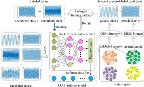
Through exploiting the unlabelled dataset $D_u$, the SSAE-Softmax classifier is then iteratively updated by two steps, i.e. the pseudo label prediction and model retraining, to minimise the following objective function: (2) $\begin{array}{rl}& \underset{{\mathit{P}}_{\mathit{f}},{\mathit{P}}_{\mathit{c}},{\phi }_j,{\tilde{h}}_j}{min}\{\sum _{j=1}^{N_l}\ell (c\text{(}{\mathit{P}}_{\mathit{c}};f\text{(}{\mathit{P}}_{\mathit{f}};s_j\text{)),}{h}_j)\\ & +\sum _{j=N_l+1}^{N_l+N_u}{\phi }_j\ell (c\text{(}{\mathit{P}}_{\mathit{c}};f\text{(}{\mathit{P}}_{\mathit{f}};s_j\text{)),}{\tilde{h}}_j)\}\end{array}$(2) where ${\tilde{h}}_j$ represents the predicted pseudo label for the j-th unlabelled sample. ${\phi }_j$ is a binary variable that is equal to one if and only if the suffered loss of the pseudo-labelled sample $(s_j,{\tilde{h}}_j)$ is adopted in the optimization process.

In the pseudo label prediction step, the trained SSAE model, namely the function $f\text{(}{\mathit{P}}_{\mathit{f}};\cdot \text{)}$, is used to embed each labelled and unlabelled sample into a feature space. The proposed DBSC strategy is then employed to generate pseudo label for each unlabelled sample according to the Euclidean distance between the unlabelled sample and each labelled sample. In subsequence, a set of pseudo-labelled candidates is selected using the DBSC strategy as: (3) $\mathrm{\Psi }=\left\{\right(s_j,{\tilde{h}}_j)|{\phi }_j=1,N_l+1\le j\le N_l+N_u\}$(3)

Note that the size of $\mathrm{\Psi }$ in each generation is controlled by the GEM strategy. In the model retraining step, an enlarged training dataset $\mathrm{\Omega }$ is obtained by merging the initial labelled dataset $D_l$ and the set $\mathrm{\Psi }$, i.e. $\mathrm{\Omega }=D_l\cup \mathrm{\Psi }$. The set $\mathrm{\Omega }$ is subsequently used to retrain the SSAE-Softmax model so as to learn a more robust classifier.

2.2 SSAE-Softmax classifier

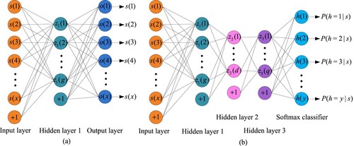
The training process of the SSAE-Softmax classifier on the initial labelled dataset or the enlarged training dataset is comprised of unsupervised pre-training followed by supervised fine-tuning. The SSAE model is established by stacking multiple trained sparse auto-encoders (SAEs). For any two consecutive SAEs in SSAE, the extracted features from the former one are used as the input data of the later one. SAE, shown in Figure 2(a), is a symmetrical structure neural network that trained to perfectly reconstruct the input data at the output layer through encoder and decoder processes, and the hidden layer in a trained SAE is then viewed as the extracted features of the input data. The detailed unsupervised training process of SAE can be referred to (Long et al. 2021). After unsupervised pre-training of SSAE, a Softmax classifier, i.e. a fully-connected layer, is stacked behind the last hidden layer of SSAE. The supervised fine-tuning of SSAE-Softmax classifier is finally performed using the back-propagation algorithm (Rumelhart, Hinton, and Williams 1986) to identify different kinds of operational states. The structure of the SSAE-Softmax classifier is shown in Figure 2(b).

Figure 2. Structure of SAE and SSAE-Softmax neural network: (a) symmetrical structure neural network of SAE, where $x$ is the dimension of each sample, $g$ is the number of neurons in the hidden layer 1; and (b) structure of SSAE-Softmax classifier, where $d$ and $q$ are the number of neurons in the hidden layer 2 and hidden layer 3, respectively, $P(h=i|x)$ denotes the probability that $s$ is classified as operational state $i$ ($i=1,2,\dots ,y$).

Two subfigures, where the first one is the symmetrical structure neural network of SAE, and the second one is the structure of SSAE-Softmax classifier.

3. The proposed GEM and DBSC

As shown in Figure 1, how to select pseudo-labelled samples into set $\mathrm{\Psi }$ in each generation has a great impact on the performance of SSDL. Therefore, two significant problems related to this procedure need to be appropriately dealt with. One is how to determine the size of $\mathrm{\Psi }$, and the other is which sampling criterion is effective for selecting candidates.

For fault diagnosis problems with a small number of labelled samples, it is difficult to train a good pseudo-label prediction model at the early iterations. Therefore, at this stage, incorporating excessive pseudo-labelled samples into set $\mathrm{\Psi }$ is irrational. Moreover, sample imbalance, i.e. the number of samples of different categories varies greatly, should be avoided in the sampling process because it will generally cause significant interference to the learning process of a classifier. With respect to the self-training for a semi-supervised classification problem, the classification loss is a simple and versatile sampling criterion. However, it is far away to train an effective pseudo-label classifier for fault diagnosis problems, where each class has a small number of labelled samples. Thus, in the case that each sample may have a high classification loss, i.e. low prediction accuracy, it is not a high identification method to select samples by comparing the classification loss difference between samples.

In this paper, the GEM strategy and DBSC strategy are proposed to address the abovementioned problems. The proposed GEM is a dynamic sampling strategy, which increases the number of pseudo-labelled samples in set $\mathrm{\Psi }$ steadily during iterations. The GEM strategy begins with a small-size subset of pseudo-labelled samples in the initial iteration. Since the SSAE-Softmax classifier becomes more discriminative and robust with the iteration of training process, more information-rich and diverse samples can be incorporated into $\mathrm{\Psi }$ in the following iterations. In addition, to avoid sample imbalance in the training dataset, at each iteration, an equal number of samples is selected by the GEM strategy for each class in set $\mathrm{\Psi }$.

Instead of classification loss, the proposed DBSC strategy adopts the Euclidean distance in the deep feature space as the confidence estimation for pseudo-label prediction. Considering that similar samples always have similar feature representations, the Nearest Neighbors classifier is employed to assign the label for each unlabelled sample by its nearest labelled sample based on their Euclidean distances in the deep feature space. The confidence estimation of pseudo-label is also defined as the Euclidean distance between the unlabelled sample and its nearest labelled one. Therefore, in the candidate selection process, equal number of top reliable pseudo-labelled samples is selected for each class according to their pseudo-label estimation confidence.

More formally, since the trained SSAE model, i.e. the function $f\text{(}{\mathit{P}}_{\mathit{f}};\cdot \text{)}$, is used as the feature extractor, the estimation confidence for each unlabelled sample $s_j\in D_u$ is defined as the minimum Euclidean distance between $s_j$ and an arbitrary labelled sample $s_k\in D_l$ in the feature space. Therefore, the estimation confidence and pseudo-label parameterised by ${\mathit{P}}_{\mathit{f}}$ of $s_j$ can be described by the following formulas (4) and (5), respectively. (4) $\begin{array}{rl}e({\mathit{P}}_{\mathit{f}};s_j)& =\underset{s_k\in D_l}{min}||f\text{(}{\mathit{P}}_{\mathit{f}};s_j\text{) - }f\text{(}{\mathit{P}}_{\mathit{f}};s_k\text{)}|{|}_2\end{array}$(4) (5) $\begin{array}{rl}\tilde{h}({\mathit{P}}_{\mathit{f}};s_j)& =label(\underset{s_k\in D_l}{\arg min}||f\text{(}{\mathit{P}}_{\mathit{f}};s_j\text{) - }f\text{(}{\mathit{P}}_{\mathit{f}};s_k\text{)}|{|}_2)\end{array}$(5) where the function $label\left(\right)$ denotes the label extraction function for samples, namely $label\left(s_j\right)=h_j$.

As shown in Equation (3), selecting set $\mathrm{\Psi }$ means determining the value of the binary variable ${\phi }_j$ for each pseudo-labelled sample. For ease of description, we use $\mathit{\phi }$ to represent all the binary variable values of the pseudo-labelled samples in set $D_u$. The selection indicator ${\mathit{\phi }}_{i,t}$ determined for the operational state $i$ ($i=1,2,\dots ,y$) at the iteration step $t$ can be calculated as: (6) ${\mathit{\phi }}_{i,t}=\underset{||{\mathit{\phi }}_{i,t}|{|}_0={\eta }_t/y\mathrm{\&}label\left(s_j\right)=i}{\arg min}\sum _{j=N_l+1}^{N_l+N_u}{\phi }_{j}e({\mathit{P}}_{\mathit{f}};s_j)$(6) where ${\eta }_t$ represents the size of set $\mathrm{\Psi }$ at the iteration step $t$. The Equation (6) is used to ensure that equal number of top reliable pseudo-labelled samples is selected for each class. Based on the selection indicators of all the classes, the selection indicator ${\mathit{\phi }}_t$ used for set $\mathrm{\Psi }$ is generated as: (7) ${\mathit{\phi }}_t={\mathit{\phi }}_{1,t}\vee {\mathit{\phi }}_{2,t}\vee \dots \vee {\mathit{\phi }}_{y,t}$(7) where $\vee$ is the logic OR operator between sets. For example, $\{0,1,0,0\}\vee \{0,0,1,0\}\vee \{1,0,0,0\}=\{1,1,1,0\}$. As iteration step $t$ increases, a enlarging factor $\xi \in (0,1)$ is determined to enlarge the size of $\mathrm{\Psi }$ as: (8) ${\eta }_t={\eta }_{t-1}+\xi N_u$(8) where $\xi$ is a predetermined parameter used to control the speed of enlarging the size of set $\mathrm{\Psi }$ during iterations. The influence of parameter $\xi$ on the performance of SSDL will be analysed in detail in the experimental section. Obviously, the Equation (8) guarantees the dynamic sampling required by the GEM strategy.

4. Procedure of the proposed SSDL for machinery fault diagnosis

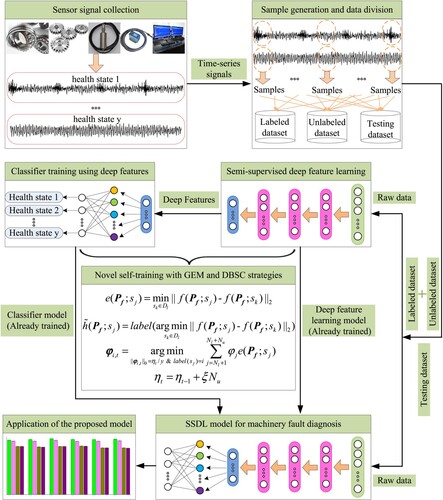
Based on all the components introduced above, the flowchart of constructing SSDL model for machinery fault diagnosis is shown in Figure 3 and its general procedure is described as bellow.

1. Step 1: Collect sensor signals (e.g. acceleration, attitude) of mechanical equipment in different health states;

2. Step 2: Employ window slicing technique on the time-series signals to generate samples;

3. Step 3: For the samples of each health state, randomly select few samples into the labelled dataset $D_l$, randomly select abundant samples with removed state labels into the unlabelled dataset $D_u$, and put the remaining samples into the testing dataset $D_t$;

4. Step 4: Initialise a set ${\mathit{\phi }}_1$ of $N_u$ zero values, iteration step $t=1$, sampling size ${\eta }_1=\xi \cdot N_u$, the best diagnostic performance ${\text{β}}^{\ast }=0$;

5. Step 5: If ${\eta }_t\le N_u$, go to Setp 6; otherwise, go to Setp 16;

6. Step 6: Select the set of pseudo-labelled candidates ${\mathrm{\Psi }}_t$ using Equation (3);

7. Step 7: Generate the enlarged training dataset ${\mathrm{\Omega }}_t=D_l\cup {\mathrm{\Psi }}_t$;

8. Step 8: Train the SSAE-Softmax model $c_t$ based on ${\mathrm{\Omega }}_t$;

9. Step 9: Obtain the diagnostic performance ${\text{β}}_t$ of model $c_t$ on $D_t$;

10. Step 10: If ${\text{β}}_t>\text{β}\ast$, go to Step 11; otherwise, go to Setp 12;

11. Step 11: Save the best diagnostic performance ${\text{β}}^{\ast }={\text{β}}_t$, the best model $c^{\ast }=c_t$;

12. Step 12: Obtain the pseudo-labels of all samples in $D_u$ using Equation (5);

13. Step 13: $t=t+1$;

14. Step 14: Update the selection indicator ${\mathit{\phi }}_t$ using Equation (7);

15. Step 15: Enlarge the sampling number ${\eta }_t={\eta }_{t-1}+\xi \cdot N_u$, go to Setp 5;

16. Step 16: Output $\text{β}\ast$ and $c\ast$.

Figure 3. Flowchart of constructing SSDL model for machinery fault diagnosis.

Flowchart of constructing SSDL model for machinery fault diagnosis, which contains the sensor signal collection, sample generation and data division, semi-supervised deep feature learning, classifier training using deep features, SSDL model for machinery fault diagnosis, and application of the proposed model.

5. Experiments and discussion

5.1 Experimental data preparation

To evaluate the performance and robustness of the proposed SSDL, two experimental cases related to the fault diagnosis of a benchmark bearing and a delta 3-D printer were prepared. The experimental data of bearing faults was downloaded from the Case Western Reserve University Bearing Data Center (n.d.), which is a benchmark dataset that widely used in this field. The experimental data of the delta 3-D printer faults was acquired from a test-rig constructed by our research group.

5.1.1 Benchmark bearing data

The main components of the test-rig used for collecting bearing data include a 2-hp motor, a torque transducer, a dynamometer, and control electronics. Single-point faults with diameters of 7, 14, and 21 mils were separately seeded on the test bearings at different locations including the inner raceway (IR), ball (BA), 3 o’clock of outer raceway (OR-3), 6 o’clock of outer raceway (OR-6), and 12 o’clock of outer raceway (OR-12), respectively. Vibration data was collected using an accelerometer with the sampling frequency of 12 kHz for motor speed set to 1797 RPM. In this study, four datasets shown in Table 1 are set up, including different fault locations (L) and different fault diameters (D). In a dataset, each operational state (O) contains 300 samples, and each sample is a collected vibration signal segment including 400 sampling data points. Note that the notation ‘N’ in the column L denotes the normal state. For each state O, 10 samples are randomly selected as the labelled dataset for training, 150 samples with removed operational state labels are randomly selected as the unlabelled dataset for training, and the remaining 140 are used for testing.

Table 1. Description of the four datasets for bearing fault diagnosis.

Dataset 1 (BD-1)			Dataset 2 (BD-2)			Dataset 3 (BD-3)			Dataset 4 (BD-4)
O	L	D	O	L	D	O	L	D	O	L	D
1	N	0	1	N	0	1	N	0	1	N	0
2	IR	7	2	IR	7	2	IR	7	2	IR	7
3	BA	7	3	IR	14	3	BA	7	3	BA	7
4	OR-3	7	4	IR	21	4	IR	14	4	OR-6	7
–	–	–	–	–	–	5	BA	14	5	IR	14
–	–	–	–	–	–	6	IR	21	6	BA	14
–	–	–	–	–	–	7	BA	21	7	OR-6	14
–	–	–	–	–	–	–	–	–	8	IR	21
–	–	–	–	–	–	–	–	–	9	BA	21
–	–	–	–	–	–	–	–	–	10	OR-6	21

5.1.2 Delta 3-D printer data

As shown in Figure 4(a), the test-rig constructed by our group for the fault diagnosis of 3-D printers consists of a delta 3-D printer, an attitude sensor, and a laptop. Considering that the faults of mechanical transmission can be reflected by the attitude of the moving platform, as shown in Figure 4(b), one attitude sensor was installed on the moving platform of 3-D printer to collect attitude data under different operational states. The attitude sensor is a three-dimensional motion attitude measurement system, which can obtain 12-channel signals including 3-channel angular velocity signals, 3-channel vibratory acceleration ones, 3-channel magnetic field intensity ones and 3-channel attitude angle ones. Note that a low-cost attitude sensor (BWT901) was used in the experiments, which is beneficial to verify the performance of the algorithm because the noise of data will be increased. There are three synchronous belts (denoted from SB-1 to SB-3) and 12 joint bearings (denoted from JB-1 to JB-12) in the delta 3-D printer. Different fault states were simulated by relaxing the length of teeth of each synchronous belt by three teeth (4.5 mm). In addition, the screw (0.700 mm pitch) of each joint bearing was loosened a 0.25-turn to simulate 0.175 mm clearance. Figure 4(c)-(d) shows the normal state and fault state of a synchronous belt and a joint bearing, respectively. As shown in Table 2, four datasets are formed by combining different states. In a dataset, each state O contains 720 samples, and each sample is a collected 12-channel signal segment including 45 sampling data points. For each state O, 10 samples are randomly selected as the labelled dataset for training, 300 samples with removed operational state labels are randomly selected as the unlabelled dataset for training, and the remaining 410 are used for testing.

Figure 4. Experimental data preparation for delta 3-D printer: (a) test-rig; (b) installed attitude sensor; (c) normal and fault state of a synchronous belt; and (d) normal and fault state of a joint bearing screw.

Four subfigures, where the first one is the test-rig of a delta 3-D printer, the second one is the attitude sensor, the third one is the normal and fault state of a synchronous belt, the last one is the normal and fault state of a joint bearing screw.

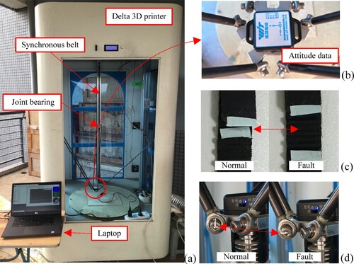
Table 2. Description of the four datasets for 3-D printer fault diagnosis.

Dataset 1 (PD-1)		Dataset 2 (PD-2)		Dataset 3 (PD-3)		Dataset 4 (PD-4)
O	State	O	State	O	State	O	State
1	N	1	N	1	N	1	N
2	JB-1	2	JB-1	2	JB-1	2	JB-1
3	JB-2	3	JB-2	3	JB-2	3	JB-2
4	JB-3	4	JB-3	4	JB-3	4	JB-3
–	–	5	JB-4	5	JB-4	5	JB-4
–	–	6	JB-5	6	SB-1	6	JB-5
–	–	–	–	7	SB-2	7	JB-6
–	–	–	–	8	SB-3	8	SB-1
–	–	–	–	–	–	9	SB-2
–	–	–	–	–	–	10	SB-3

5.2 Hyper-parameter analysis

Two hyper-parameters (i.e. the network architecture of SSAE-Softmax model, which is denoted as na, and the enlarging factor $\xi$) were analysed because they have a great impact on the performance of the proposed SSDL. Taking the dataset BD-1 as an example, the diagnosis accuracies of SSDL under different hyper-parameter combinations are described in Table 3. Note that the network architecture of SSAE-Softmax is denoted as the number of hidden layers and the number of neurons in each hidden layer. For example, the na = [50-50-50] in Table 3 implies that the model has three hidden layers and each hidden layer has 50 neurons. The other hyper-parameters including the batch size, iterations, and learning rate for the training algorithm of SSAE-Softmax model were set as 10, 100, and 0.5, respectively, in the following experiments. All the SSDLs under different hyper-parameter combinations were run independently five times on dataset BD-1 to reduce the effect of randomness. Therefore, the average diagnosis accuracies (avg) and the standard deviations (std) are also reported in Table 3.

Table 3. Diagnosis accuracies of SSDL under different combinations of network architecture and enlarging factor.

	$\xi$=1/3		$\xi$=1/5		$\xi$=1/10		$\xi$=1/15		$\xi$=1/30
Network architecture	avg	std	avg	std	avg	std	avg	std	avg	std
[100]	84.64	8.46	87.38	4.84	88.57	5.04	86.25	6.57	91.49	5.86
[200]	90.18	1.97	90.54	0.68	90.14	0.49	91.72	2.10	91.88	1.17
[300]	83.75	0.83	89.73	2.41	89.38	3.31	90.18	0.74	90.45	1.52
[400]	84.94	2.09	87.50	1.51	92.50	3.04	88.04	1.03	91.25	0.89
[500]	87.68	0.82	86.52	0.27	91.25	3.57	87.50	3.93	90.18	0.89
[600]	82.77	6.52	89.29	3.04	91.61	0.52	91.31	6.23	90.63	5.81
[100-100]	87.50	0.76	95.24	1.17	97.44	0.14	96.13	1.43	97.97	0.33
[200-200]	94.88	2.70	96.73	1.36	96.07	0.51	96.96	0.95	98.57	0.91
[300-300]	93.04	2.46	96.25	1.30	99.64	0.38	98.87	0.73	99.52	0.55
[400-400]	92.50	1.39	96.67	0.74	99.22	0.59	98.45	2.06	99.64	0.25
[500-500]	91.31	4.26	96.61	1.82	95.12	5.27	94.11	3.79	95.45	0.45
[600-600]	93.45	1.33	94.00	2.70	96.72	2.66	95.30	2.70	96.07	1.43
[50-50-50]	87.56	2.88	88.15	6.65	94.65	2.86	98.49	0.63	96.79	1.79
[100-100-100]	90.30	1.18	95.89	0.58	95.77	1.38	98.57	1.51	98.87	0.60
[150-150-150]	91.34	2.59	93.66	2.23	93.66	0.53	95.90	1.97	95.72	2.15
[200-200-200]	92.14	2.29	93.15	2.04	94.64	2.34	96.70	0.99	95.18	0.47
[250-250-250]	91.70	2.41	94.56	2.24	93.84	1.34	96.26	0.71	98.04	1.43
[300-300-300]	94.40	1.05	95.81	1.70	98.67	0.63	97.05	2.41	97.80	2.38

Table 4. Hyper-parameter settings for all the approaches on bearing datasets.

Approach	BD-1	BD-2	BD-3	BD-4
SSDL-SS	na = [500-500]; threshold = 0.95; iter = 10;	na = [200-200-200]; threshold = 0.95; iter = 5;	na = [200-200-200]; threshold = 0.98; iter = 10;	na = [300-300]; threshold = 0.88; iter = 10;
SSDL-SC	na = [300-300]; $\xi$=1/10;	na = [300-300]; $\xi$=1/30;	na = [200-200-200]; $\xi$=1/30;	na = [250-250-250]; $\xi$=1/30;
SSDL-ES	na = [400-400]; $\xi$=1/30;	na = [50-50-50]; $\xi$=1/15;	na = [50-50-50]; $\xi$=1/30;	na = [100-100-100]; $\xi$=1/30;
SSDL	na = [300-300]; $\xi$=1/10;	na = [50-50-50]; $\xi$=1/30;	na = [300-300]; $\xi$=1/30;	na = [300-300-300]; $\xi$=1/30;

Table 5. Hyper-parameter settings for all the approaches on 3-D printer datasets.

Approach	PD-1	PD-2	PD-3	PD-4
SSDL-SS	na = [100-100-100]; threshold= 0.98; iter = 5;	na = [100-100-100]; threshold= 0.95; iter = 10;	na = [300-300]; threshold = 0.95; iter = 10;	na = [400-400]; threshold = 0.95; iter = 10;
SSDL-SC	na = [150-100]; $\xi$=1/15;	na = [200-100-100]; $\xi$=1/15;	na = [400-300]; $\xi$=1/15;	na = [400-300]; $\xi$=1/30;
SSDL-ES	na = [200-100-100]; $\xi$=1/15;	na = [200-200-100]; $\xi$=1/15;	na = [300-300]; $\xi$=1/30;	na = [400-400]; $\xi$=1/15;
SSDL	na = [100-100-100]; $\xi$=1/30;	na = [100-100-100]; $\xi$=1/30;	na = [300-300]; $\xi$=1/15;	na = [400-400]; $\xi$=1/30;

The following conclusions can be inferred from the results. On the one hand, under the same architecture, the performance of the SSDL is generally not good enough when the value of $\xi$ is large (e.g. $\xi$ = 1/3 or $\xi$ = 1/5). This is because that a large $\xi$ will urge ${\eta }_t$ to increase rapidly and unreliable pseudo-labelled data may be sampled to train the classifier at each step. On the other hand, at the same level of $\xi$, it can be seen that the performance of the SSDL was not improved monotonously with the increase of the number of hidden layers and the number of neurons in each hidden layer. Therefore, to make the SSDL have better performance, the fitting ability of the SSAE-Softmax model cannot be too strong or too weak.

5.3 Algorithm performance analysis

Compared with existing self-training semi-supervised learning approaches, GEM and DBSC strategies are two main improvements in the proposed SSDL. Therefore, in this subsection, the performance of these two strategies are analysed first. As stated before, most existing self-training semi-supervised learning approaches adopt a static sampling strategy that selecting pseudo-labelled samples into the enlarged training dataset when their prediction confidences larger than a fixed threshold (Fan et al. 2018; Ye et al. 2017). Therefore, the first contrastive approach was selected as the SSDL where the sampling strategy GEM was replaced by this static sampling strategy (denoted as SSDL-SS). As shown in Section 4, the termination condition of the iterative learning of SSDL is when the sampling size ${\eta }_t$ is greater than $N_u$. However, due to the static sampling strategy employed in SSDL-SS, a predetermined number of iterations (denoted as iter) is adopted as the termination criterion for the iterative learning of SSDL-SS. The second contrastive approach was defined as the SSDL where the sampling criterion DBSC was replaced by the widely used one (Dong et al. 2017; Fan et al. 2017) that the prediction accuracy of classifier was employed directly as the confidence estimation for pseudo-labels (denoted as SSDL-SC). It means that the pseudo-labels of samples were assigned as the predicted labels of the classifier directly in SSDL-SC. Recall that an equilibrium strategy is used in GEM to guarantee that an equal number of pseudo-labelled samples is selected for each class at each iteration. Therefore, to analyse its effectiveness, the third contrastive approach was defined as the SSDL where the equilibrium strategy was not adopted in GEM (denoted as SSDL-ES). Note that the static sampling strategy used in SSDL-SS also implies that the pseudo-labels of unlabelled samples are predicted by the classifier directly, and the equilibrium strategy is not employed in SSDL-SS either.

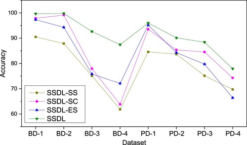
Considering the influence of hyper-parameter settings on the prediction accuracy, for fair comparison, different hyper-parameter combinations were tested first to achieve the optimal hyper-parameter setting, as shown in Tables 4 and 5, for all the above contrastive approaches on each dataset. The comparative results of five trials on the bearing testing datasets and 3-D printer testing datasets are described in Figure 5. From these results, one can find that the performance of the proposed SSDL are much better than that of SSDL-SS, SSDL-SC, and SSDL-ES, which demonstrates the effectiveness of the strategies designed in SSDL for semi-supervised learning.

Figure 5. The prediction accuracies obtained by all the algorithms on each testing dataset.

The prediction accuracies obtained by the SSDL-SS, SSDL-SC, SSDL-ES, and SSDL on datasets BD-1, BD-2, BD-3, BD-4, PD-1, PD-2, PD-3, and PD-4.

Although the labels of samples in the unlabelled dataset are removed and cannot be used in the training process, they can be used to calculate the following two metrics, namely the prediction accuracy of the model on the unlabelled dataset D_u (denoted as Accu) and the accuracy of the selected pseudo-labelled candidates in set $\mathrm{\Psi }$ (denoted as Accs), at each iteration to observe the performance improvement of the model during the iterative learning process: (9) $\begin{array}{rl}Accu& =100\times right\mathrm{\_}predicted\mathrm{\_}labels/|D_u|\end{array}$(9) (10) $\begin{array}{rl}Accs& =100\times right\mathrm{\_}pseudo-labels/|\mathrm{\Psi }|\end{array}$(10) where the right_predicted_labels denotes the number of samples in set D_u whose labels are predicted right by the SSAE-Softmax classifier, the right_pseudo-labels denotes the number of samples in set $\mathrm{\Psi }$ whose pseudo labels are consistent with their true labels, $|D_u|$ and $|\mathrm{\Psi }|$ denote the size of D_u and $\mathrm{\Psi }$, respectively.

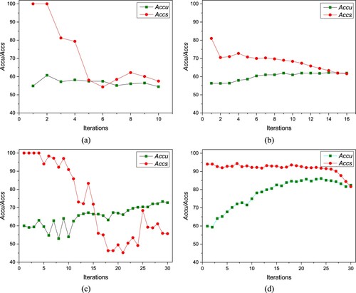
Owing to space constraints, as shown in Figures 6 and 7, we only show the iterative Accu and Accs values of the SSDL-SS, SSDL-SC, SSDL-ES and SSDL on the BD-1 and BD-4 datasets. We can find that the Accs value drops a lot in the iterative learning process of SSDL-SS, which means that the pseudo labels of most of the candidates in set $\mathrm{\Psi }$ at the later iterations are incorrect. This is the reason why the Accu value of SSDL-SS stagnates in the iterative learning process and the poor performance of SSDL-SS achieved on the testing datasets. There are two possible reasons for the degradation of Accs value of SSDL-SS. The first one is that the pseudo-labels predicted by the classifier are not reliable sometimes. This phenomenon can also be found by observing the Accs value of SSDL-SC on the dataset BD-4. The second one is that the equilibrium strategy is not adopted. Without using the equilibrium strategy, sample imbalance (i.e. the number of samples of different categories varies greatly) may occur in the enlarged training dataset $\mathrm{\Omega }$. This is not good for training a high performance classifier. This phenomenon can also be found by observing Accs and Accu values of SSDL-ES both on the datasets BD-1 and BD-4.

Figure 6. The iterative Accu and Accs values of the contrastive approaches on the BD-1: (a) SSDL-SS; (b) SSDL-SC; (c) SSDL-ES; and (d) SSDL.

Four subfigures are drawn to show the iterative Accu and Accs values of the SSDL-SS, SSDL-SC, SSDL-ES, and SSDL on dataset BD-1.

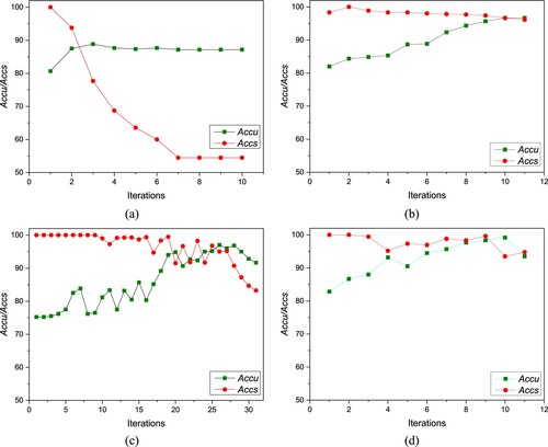
Figure 7. The iterative Accu and Accs values of the contrastive approaches on the BD-4: (a) SSDL-SS; (b) SSDL-SC; (c) SSDL-ES; and (d) SSDL.

Four subfigures are drawn to show the iterative Accu and Accs values of the SSDL-SS, SSDL-SC, SSDL-ES, and SSDL on dataset BD-4.

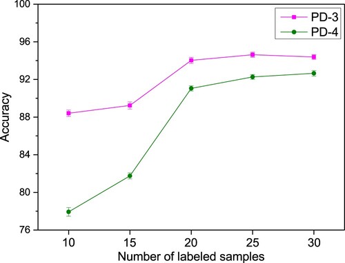
In addition to the above performance analysis of each improved strategy of SSDL, the effect of the size of the labelled dataset $D_l$ on the performance of the proposed SSDL is also analysed. Taking datasets PD-3 and PD-4 as examples, recall that only about 3.2% of the samples in these training datasets are labelled (10 labelled samples and 300 unlabelled samples). Figure 8 shows the prediction accuracies of SSDL when the number of labelled samples is 10, 15, 20, 25 and 30, respectively. It can be clearly seen that the diagnostic accuracy of SSDL has been greatly improved with the increase of labelled samples, and satisfying performance can still be achieved at a relatively low ratio of labelled samples.

Figure 8. The prediction accuracies obtained by SSDL under different number of labelled samples on datasets PD-3 and PD-4.

The prediction accuracies obtained by SSDL on datasets PD-3 and PD-4 when the number of labelled samples is 10, 15, 20, 25, and 30.

5.4 Comparisons with the state-of-the-art

In order to further study the performance of the proposed SSDL, several state-of-the-art semi-supervised learning approaches including mixmatch (Berthelot et al. 2019), mean teachers (MT for short) (Tarvainen and Valpola 2017), and learning to impute (LTI for short) (Li, Foo, and Bilen 2020) were employed for comparison. SSAE-based deep deep neural networks are always adopted as the backbone architecture for competitive fault diagnosis models (Shao et al. 2018). Therefore, besides the above three semi-supervised learning approaches, two baseline models trained in supervised learning fashion, denoted as BFS and BSU, were also constructed and used for comparison. BFS denotes that we only take the labelled dataset $D_l$ to train a SSAE-Softmax classifier without exploiting the unlabelled dataset $D_u$, while BSU means that all the samples in $D_l$ and $D_u$ are labelled and used to train a SSAE-Softmax classifier.

The average diagnosis accuracy and standard deviations obtained by each approach in five independent repeated experiments are depicted in Table 6. From this table, we can observe that the proposed SSDL can obtain higher average diagnosis accuracy than the other three state-of-the-art semi-supervised learning approaches (i.e. mixmatch, MT and LTI) on each dataset. The overall average diagnosis accuracy obtained by SSDL is 91.49%. It is better than that of the LTI, mixmatch and MT, whose overall average diagnosis accuracy is 89.44%, 88.40% and 86.91%, respectively. The experimental results demonstrate the superiority of the proposed SSDL for machinery fault diagnosis.

Table 6. Comprehensive comparison of diagnosis accuracy.

Dataset	mixmatch	MT	LTI	SSDL	BFS	BSU
BD-1	98.46 ± 0.13	98.29 ± 0.21	99.02 ± 0.18	99.64 ± 0.03	82.32 ± 0.27	100.00 ± 0.00
BD-2	98.41 ± 0.20	97.54 ± 0.19	98.76 ± 0.14	99.78 ± 0.02	84.47 ± 0.15	100.00 ± 0.00
BD-3	89.17 ± 0.36	87.28 ± 0.35	90.69 ± 0.32	92.65 ± 0.25	72.04 ± 0.31	97.02 ± 0.14
BD-4	83.85 ± 0.31	81.19 ± 0.41	84.12 ± 0.34	87.43 ± 0.21	59.43 ± 0.28	96.57 ± 0.18
PD-1	93.89 ± 0.26	93.26 ± 0.28	95.04 ± 0.23	95.98 ± 0.14	82.99 ± 0.17	98.35 ± 0.09
PD-2	87.18 ± 0.30	85.36 ± 0.33	88.21 ± 0.21	90.12 ± 0.23	81.22 ± 0.26	96.58 ± 0.13
PD-3	82.45 ± 0.27	79.43 ± 0.36	84.67 ± 0.29	88.41 ± 0.18	72.24 ± 0.36	95.83 ± 0.18
PD-4	73.76 ± 0.29	72.89 ± 0.33	75.03 ± 0.24	77.93 ± 0.21	61.85 ± 0.34	93.68 ± 0.21

Through comparing the results of SSDL with that of BFS, one can find that the prediction accuracy of the model can be greatly improved by exploiting the unlabelled dataset. Specifically, the proposed SSDL achieves about 8.9–28.0 points improvements over the BFS on all the testing datasets. With respect to the comparison between the results of SSDL and BSU, it can be seen that the performance of SSDL is close to that of the totally supervised learning on most datasets (e.g. BD-1, BD-2, BD-3, PD-1, and PD-2), proving the high effectiveness of the proposed SSDL for fault diagnosis with few labelled samples. However, for some complicated datasets (e.g. BD-4, PD-3 and PD-4), there is still a big gap between SSDL and BSU. Therefore, continuously improve the performance of SSDL in dealing with large and complex data is the direction of our future study.

6. Conclusions

A large number of labelled samples are always required by most of existing data-driven fault diagnosis approaches designed under supervised learning frameworks. However, labeling large number of samples to different operational states is always time-consuming and costly, sometimes even impossible, for machinery fault diagnosis. To solve this problem, a novel self-training semi-supervised deep learning (SSDL) approach is proposed in this paper. The SSDL approach adopts a gradually exploiting mechanism (GEM) to start with few reliable unlabelled samples and gradually increasing its quantity for model updating. Moreover, a distance-based sampling criterion (DBSC) is presented to remarkably improve the performance of label estimation. The influence of hyper-parameters on the performance of the proposed SSDL is analysed in the experiments. The superiority of the present SSDL in dealing with fault diagnosis problems with few labelled and abundant unlabelled samples is also demonstrated by comparing with other state-of-the-art semi-supervised learning approaches. There are in general three contributions for the addressed work: (1) we propose the GEM strategy for semi-supervised self-training to better exploit the unlabelled samples; (2) we design the DBSC for label estimation to remarkably improve the performance of pseudo-labelled sample selection in the iterative learning process; and (3) an integrated SSDL based on the GEM and DBSC is proposed for dealing with the machinery fault diagnosis with few labelled data. In the future studies, the proposed SSDL will be explored to extend its application for other fault diagnosis problems considering more realistic situations, such as variable working condition and unknown abnormality identification.

Acknowledgments

The valuable comments and suggestions from the editors and the anonymous reviewers are very much appreciated.

Disclosure statement

No potential conflict of interest was reported by the author(s).

Additional information

Funding

This research is partially supported by the National Natural Science Foundation of China (72171049, 52175080, 52005103), the Guangdong Basic and Applied Basic Research Foundation (2019B1515120095), and the Intelligent Manufacturing PHM Innovation Team Program (2018KCXTD029, TDYB2019010).

Notes on contributors

Jianyu Long

Jianyu Long received the B.E. degree and the Ph.D. degree in Metallurgical Engineering from Chongqing University, Chongqing, China, in 2012 and 2017, respectively. He is currently an associate professor with the School of Mechanical Engineering, Dongguan University of Technology, Dongguan, China. His research interests include machine learning, prognostics and system health management.

Yibin Chen

Yibin Chen received the B.E. degree in Traffic Engineering from Wuyi University, Jiangmen, China. He is currently working toward the Master degree with the College of Mechatronics and Control Engineering, Shenzhen University, Shenzhen, China. His research interests include fault diagnosis and few shot learning.

Zhe Yang

Zhe Yang received the B.E. degree in Measurement and Control and Instrument, the M.Sc. degree in Mechanical Engineering from Xi’an Jiaotong University, Xi’an, China, in 2012 and 2015, respectively, and the Ph.D. degree in Mechanical Engineering from Politecnico di Milano, Milan, Italy, in 2020. He is currently a Postdoctoral Fellow with the Dongguan University of Technology, Dongguan, China. His research interests include the development of methods for prognostics and system health management.

Yunwei Huang

Yunwei Huang received the B.E. degree and the Ph.D. degree in Metallurgical Engineering from Chongqing University, Chongqing, China, in 2013 and 2020, respectively. He is currently a Postdoctoral Fellow with the Dongguan University of Technology, Dongguan, China. His research interests include few shot learning and artificial intelligence.

Chuan Li

Chuan Li received his Ph.D. degree from the Chongqing University, China, in 2007. He has been successively a Postdoctoral Fellow with the University of Ottawa, Canada, a Research Professor with the Korea University, South Korea, and a Senior Research Associate with the City University of Hong Kong, China. He is currently a Professor with the School of Mechanical Engineering, Dongguan University of Technology, Dongguan, China. His research interests include prognostics & health management, and intelligent systems.

References

- Agrawala, A. K. 1970. “Learning with a Probabilistic Teacher.” IEEE Transactions on Information Theory 16: 373–379.
- Artigao, E., A. Honrubia-Escribano, and E. Gomez-Lazaro. 2020. “In-Service Wind Turbine DFIG Diagnosis Using Current Signature Analysis.” IEEE Transactions on Industrial Electronics 67: 2262–2271.
- Belkin, M., P. Niyogi, and V. Sindhwani. 2006. “Manifold Regularization: A Geometric Framework for Learning from Labeled and Unlabeled Examples.” Journal of Machine Learning Research 7: 2399–2434.
- Bennett, K. P., and A. Demiriz. 1999. “Semi-supervised Support Vector Machines.” Proceedings of the Neural Information Processing Systems, 368–374.
- Berthelot, D., N. Carlini, I. Goodfellow, N. Papernot, A. Oliver, and C. Raffel . 2019. MixMatch: A holistic approach to semi-supervised learning: arXiv:1905.02249.
- Blum, A., and T. M. Mitchell. 1998. “Combining Labeled and Unlabeled Data with co-Training.” Proceedings of the Eleventh Annual Conference on Computational Learning Theory, 92–100.
- Case Western Reserve University. n.d. Bearing Data Center. https://csegroups.case.edu/bearingdatacenter/home.
- Dong, X., D. Meng, F. Ma, and Y. Yang. 2017. “A Dual-Network Progressive Approach to Weakly Supervised Object Detection.” Proceedings of the ACM International Conference on Multimedia, 279–287.
- Fan, H., X. Chang, D. Cheng, Y. Yang, D. Xu, and A. G. Hauptmann. 2017. “Complex Event Detection by Identifying Reliable Shots from Untrimmed Videos.” Proceedings of the IEEE International Conference on Computer Vision, 736–744.
- Fan, H., L. Zheng, C. Yan, and Y. Yang . 2018. “Unsupervised Person re-Identification: Clustering and Fine-Tuning.” Acm Transactions on Multimedia Computing Communications and Applications 83: 1–18.
- Gao, Z., C. Cecati, and S. X. Ding. 2015a. “A Survey of Fault Diagnosis and Fault-Tolerant Techniques-Part i: Fault Diagnosis with Model-Based and Signal-Based Approaches.” IEEE Transactions on Industrial Electronics 62: 3757–3767.
- Gao, Z., C. Cecati, and S. X. Ding. 2015b. “A Survey of Fault Diagnosis and Fault-Tolerant Techniques-Part ii: Fault Diagnosis with Knowledge-Based and Hybrid/Active Approaches.” IEEE Transactions on Industrial Electronics 62: 3768–3774.
- Hanachi, H., J. Liu, I. Y. Kim, and C. K. Mechefske. 2019. “Hybrid Sequential Fault Estimation for Multi-Mode Diagnosis of gas Turbine Engines.” Mechanical Systems and Signal Processing 115: 255–268.
- Hu, Y., P. Baraldi, F. Di Maio, and E. Zio. 2017. “A Systematic Semi-Supervised Self-Adaptable Fault Diagnostics Approach in an Evolving Environment.” Mechanical Systems and Signal Processing 88: 413–427.
- Jeong, I. J., V. J. Leon, and J. R. Villalobos. 2007. “Integrated Decision-Support System for Diagnosis, Maintenance Planning, and Scheduling of Manufacturing Systems.” International Journal of Production Research 45: 267–285.
- Lee, J., B. Park, and C. Lee. 2020. “Fault Diagnosis Based on the Quantification of the Fault Features in a Rotary Machine.” Applied Soft Computing 97: 106726.
- Lei, Y., B. Yang, X. Jiang, F. Jia, N. Li, and A. K. Nandi. 2020. “Applications of Machine Learning to Machine Fault Diagnosis: A Review and Roadmap.” Mechanical Systems and Signal Processing 138: 106587.
- Li, W., C. Foo, and H. Bilen . 2020. Learning to impute: a general framework for semi-supervised learning: arXiv:1912.10364.
- Long, J., J. Mou, L. Zhang, S. Zhang, and C. Li. 2021. “Attitude Data-Based Deep Hybrid Learning Architecture for Intelligent Fault Diagnosis of Multi-Joint Industrial Robots.” Journal of Manufacturing Systems 61: 736–745.
- Long, J. Y., Z. Z. Sun, C. Li, Y. Hong, Y. Bai, and S. H. Zhang. 2020a. “A Novel Sparse Echo Autoencoder Network for Data-Driven Fault Diagnosis of Delta 3-D Printers.” IEEE Transactions on Instrumentation and Measurement 69: 683–692.
- Long, J. Y., S. H. Zhang, and C. Li. 2020b. “Evolving Deep Echo State Networks for Intelligent Fault Diagnosis.” IEEE Transactions on Industrial Informatics 16: 4928–4937.
- Majdouline, I., S. Dellagi, L. Mifdal, E. M. Kibbou, and A. Moufki. 2021. “Integrated Production-Maintenance Strategy Considering Quality Constraints in dry Machining.” International Journal of Production Research,. Early Access.
- Nigam, K., A. McCallum, S. Thrun, and T. M. Mitchell. 2000. “Text Classification from Labeled and Unlabeled Documents Using EM.” Machine Learning 39: 103–134.
- Potocnik, P., and E. Govekar. 2017. “Semi-supervised Vibration-Based Classification and Condition Monitoring of Compressors.” Mechanical Systems and Signal Processing 93: 51–65.
- Razavi-Far, R., E. Hallaji, M. Farajzadeh-Zanjani, M. Saif, S. H. Kia, H. Henao, and G.-A. Capolino. 2019. “Information Fusion and Semi-Supervised Deep Learning Scheme for Diagnosing Gear Faults in Induction Machine Systems.” IEEE Transactions on Industrial Electronics 66: 6331–6342.
- Rosenberg, C., M. Hebert, and H. Schneiderman. 2005. Semi-supervised self-training of object detection models, the 7th IEEE Workshop on Applications of Computer Vision: 29-36.
- Rumelhart, D. E., G. E. Hinton, and R. J. Williams. 1986. “Learning Representations by Back-Propagating Errors.” Nature 323: 533–536.
- Shao, H. D., H. K. Jiang, Y. Lin, and X. Q. Li. 2018. “A Novel Method for Intelligent Fault Diagnosis of Rolling Bearings Using Ensemble Deep Auto-Encoders.” Mechanical Systems and Signal Processing 102: 278–297.
- Shao, H. D., J. Lin, L. W. Zhang, D. Galar, and U. Kumar. 2021a. “A Novel Approach of Multisensory Fusion to Collaborative Fault Diagnosis in Maintenance.” Information Fusion 74: 65–76.
- Shao, H., M. Xia, G. Han, Y. Zhang, and J. Wan. 2021b. “Intelligent Fault Diagnosis of Rotor-Bearing System Under Varying Working Conditions with Modified Transfer Convolutional Neural Network and Thermal Images.” IEEE Transactions on Industrial Informatics 17: 3488–3496.
- Tarvainen, A., and H. Valpola. 2017. “Mean Teachers are Better Role Models: Weight-Averaged Consistency Targets Improve Semi-Supervised Deep Learning Results.” Proceedings of the Neural Information Processing Systems, 1195–1204.
- Wang, Z., Q. Liu, H. Chen, and X. Chu. 2021. “A Deformable CNN-DLSTM Based Transfer Learning Method for Fault Diagnosis of Rolling Bearing Under Multiple Working Conditions.” International Journal of Production Research 59: 4811–4825.
- Yang, W., L. Chen, and S. Dauzere-Peres. 2021a. “A Dynamic Optimisation Approach for a Single Machine Scheduling Problem with Machine Conditions and Maintenance Decisions.” International Journal of Production Research,. Early Access.
- Yang, X., Z. Song, I. King, and Z. Xu. 2021b. A survey on deep semi-supervised learning: arXiv:2103.00550.
- Ye, M., A. J. Ma, L. Zheng, J. Li, and P. C. Yuen. 2017. “Dynamic Label Graph Matching for Unsupervised Video re-Identification.” Proceedings of the IEEE International Conference on Computer Vision, 5152–5160.
- Zhang, Y. Y., X. Y. Li, L. Gao, W. Chen, and P. G. Li. 2020. “Ensemble Deep Contractive Auto-Encoders for Intelligent Fault Diagnosis of Machines Under Noisy Environment.” Knowledge-Based Systems 196: 105764.
- Zhang, C., J. Yu, and S. Wang. 2021. “Fault Detection and Recognition of Multivariate Process Based on Feature Learning of one-Dimensional Convolutional Neural Network and Stacked Denoised Autoencoder.” International Journal of Production Research 59: 2426–2449.
- Zhao, X., M. Jia, J. Bin, T. Wang, and Z. Liu. 2020a. “Multiple-Order Graphical Deep Extreme Learning Machine for Unsupervised Fault Diagnosis of Rolling Bearing.” IEEE Transactions on Instrumentation and Measurement 70: 3506012.
- Zhao, X., M. Jia, and Z. Liu. 2021a. “Semisupervised Graph Convolution Deep Belief Network for Fault Diagnosis of Electormechanical System with Limited Labeled Data.” IEEE Transactions on Industrial Informatics 17: 5450–5460.
- Zhao, B., X. Zhang, Z. Zhan, and Q. Wu. 2021b. “Deep Multi-Scale Adversarial Network with Attention: A Novel Domain Adaptation Method for Intelligent Fault Diagnosis.” Journal of Manufacturing Systems 59: 565–576.
- Zhao, M., S. Zhong, X. Fu, B. Tang, and M. Pecht. 2020b. “Deep Residual Shrinkage Networks for Fault Diagnosis.” IEEE Transactions on Industrial Informatics 16: 4681–4690.
- Zheng, J., H. Wang, Z. Song, and Z. Ge. 2019. “Ensemble Semi-Supervised Fisher Discriminant Analysis Model for Fault Classification in Industrial Processes.” ISA Transactions 92: 109–117.